Logistic regression

Marco Baroni

Linear models in R

Outline

Logistic regression

Logistic regression in R

Further topics

Outline

Logistic regressionIntroductionThe modelEstimationLooking at and comparing fitted models

Logistic regression in R

Further topics

Outline

Logistic regressionIntroductionThe modelEstimationLooking at and comparing fitted models

Logistic regression in R

Further topics

Modeling discrete response variables

I In a very large number of problems in cognitive scienceand related fields

I the response variable is categorical, often binary (yes/no;acceptable/not acceptable; phenomenon takes place/doesnot take place)

I potentially explanatory factors (independent variables) arecategorical, numerical or both

Examples: binomial responses

I Is statement X rated as “acceptable” in the followingcondition(s)?

I Does sentence S, that has features Y, W and Z, displayphenomenon X? (linguistic corpus data!)

I Is it common for shoppers to decide to purchase the goodX given these conditions?

I Did subject make more errors in this condition?I How many people answer YES to question X in the surveyI Do old women like X more than young men?I Did the subject feel pain in this condition?I How often was reaction X triggered by these conditions?I Do children with characteristics X, Y and Z tend to have

autism?

Examples: multinomial responsesI Discrete response variable with natural ordering of the

levels:I Ratings on a 6-point scale

I Depending on the number of points on the scale, you mightalso get away with a standard linear regression

I Subjects answer YES, MAYBE, NOI Subject reaction is coded as FRIENDLY, NEUTRAL,

ANGRYI The cochlear data: experiment is set up so that possible

errors are de facto on a 7-point scaleI Discrete response variable without natural ordering:

I Subject decides to buy one of 4 different productsI We have brain scans of subjects seeing 5 different objects,

and we want to predict seen object from features of thescan

I We model the chances of developing 4 different (andmutually exclusive) psychological syndromes in terms of anumber of behavioural indicators

Binomial and multinomial logistic regression models

I Problems with binary (yes/no, success/failure,happens/does not happen) dependent variables arehandled by (binomial) logistic regression

I Problems with more than one discrete output are handledby

I ordinal logistic regression, if outputs have natural orderingI multinomial logistic regression otherwise

I The output of ordinal and especially multinomial logisticregression tends to be hard to interpret, whenever possibleI try to reduce the problem to a binary choice or a set ofbinary choices

I E.g., if output is yes/maybe/no, treat “maybe” as “yes”and/or as “no”

I Multiple binomial regressions instead of a singlemultinomial regression

I Here, I focus entirely on the binomial case

Don’t be afraid of logistic regression!

I Logistic regression is less popular than linear regressionI This might be due in part to historical reasons

I the formal theory of generalized linear models is relativelyrecent: it was developed in the early 70s

I the iterative maximum likelihood methods used for fittinglogistic regression models require more computationalpower than solving the least squares equations

I Results of logistic regression are not as straightforward tounderstand and interpret as linear regression results

I Finally, there might also be a bit of prejudice againstdiscrete data as less “scientifically credible” thanhard-science-like continuous measurements

Don’t be afraid of logistic regression!

I If it is natural to cast your problem in terms of a discretevariable, you should go ahead and use logistic regression

I Logistic regression might be trickier to work with than linearregression, but it’s still much better than pretending that thevariable is continuous or artificially re-casting the problemin terms of a continuous response

The Machine Learning angle

I Classification of a set of observations into 2 or morediscrete categories is a central task in Machine Learning

I The classic supervised learning setting:I Data points are represented by a set of features, i.e.,

discrete or continuous explanatory variablesI The “training” data also have a label indicating the class of

the data point, i.e., a discrete binomial or multinomialdependent variable

I A model (e.g., in the form of weights assigned to thedependent variables) is fitted to the training data

I The trained model is then used to predict the class ofunseen data points (where we know the values of thefeatures, but we do not have the label)

The Machine Learning angle

I Same setting of logistic regression, except that emphasis isplaced on predicting the class of unseen data, rather thanon the significance of the effect of the features/independentvariables (that are often too many – hundreds or more – tobe analyzed singularly) in discriminating the classes

I Indeed, logistic regression is also a standard technique inMachine Learning, where it is sometimes known asMaximum Entropy

Outline

Logistic regressionIntroductionThe modelEstimationLooking at and comparing fitted models

Logistic regression in R

Further topics

Ordinary linear regression

I The by now familiar model:

y = β0 + β1x1 + β2 × x2 + ...+ βnxn + ε

I Why will this not work if variable is binary (0/1)?I Why will it not work if we try to model proportions instead

of responses (e.g., proportion of YES-responses incondition C)?

Modeling log odds ratiosI Following up on the “proportion of YES-responses” idea,

let’s say that we want to model the probability of one of thetwo responses (which can be seen as the populationproportion of the relevant response for a certain choice ofthe values of the independent variables)

I Probability will range from 0 to 1, but we can look at thelogarithm of the odds ratio instead:

logit(p) = logp

1− pI This is the logarithm of the ratio of probability of

1-response to probability of 0-responseI It is arbitrary what counts as a 1-response and what counts

as a 0-response, although this might hinge on the ease ofinterpretation of the model (e.g., treating YES as the1-response will probably lead to more intuitive results thantreating NO as the 1-response)

I Log odds ratios are not the most intuitive measure (at leastfor me), but they range continuously from −∞ to +∞

From probabilities to log odds ratios

0.0 0.2 0.4 0.6 0.8 1.0

−5

05

p

logi

t(p)

The logistic regression model

I Predicting log odds ratios:

logit(p) = β0 + β1x1 + β2x2 + ...+ βnxn

I From probabilities to log odds ratios:

logit(p) = logp

1− p

I Back to probabilities:

p =elogit(p)

1 + elogit(p)

I Thus:

p =eβ0+β1x1+β2x2+...+βnxn

1 + eβ0+β1x1+β2x2+...+βnxn

From log odds ratios to probabilities

−10 −5 0 5 10

0.0

0.2

0.4

0.6

0.8

1.0

logit(p)

p

Probabilities and responses

−10 −5 0 5 10

0.0

0.2

0.4

0.6

0.8

1.0

logit(p)

p

●●● ● ●● ●● ● ●

●●●●●●●●●●

What is the relation between p and the response?

I Given a single response at a specific setting of theindependent variables, p is the p parameter of a Bernoulliprobability distribution for whether the response is 1 (YES,success, etc.) or 0 (NO, failure, etc.)

I Probability of the two possible values for the responserandom variable (1 and 0):

P(y) = py (1− p)(1−y)

I Expected value: E(y) = pI Variance: var(y) = p(1− p)

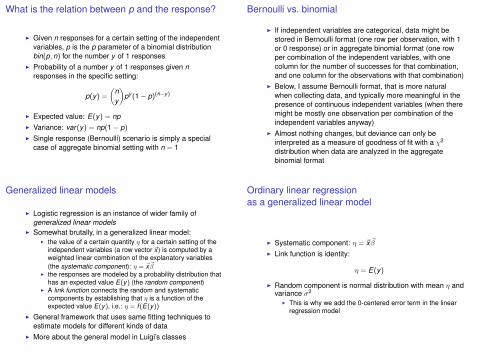
What is the relation between p and the response?

I Given n responses for a certain setting of the independentvariables, p is the p parameter of a binomial distributionbin(p,n) for the number y of 1 responses

I Probability of a number y of 1 responses given nresponses in the specific setting:

p(y) =(

ny

)py (1− p)(n−y)

I Expected value: E(y) = npI Variance: var(y) = np(1− p)I Single response (Bernoulli) scenario is simply a special

case of aggregate binomial setting with n = 1

Bernoulli vs. binomial

I If independent variables are categorical, data might bestored in Bernoulli format (one row per observation, with 1or 0 response) or in aggregate binomial format (one rowper combination of the independent variables, with onecolumn for the number of successes for that combination,and one column for the observations with that combination)

I Below, I assume Bernoulli format, that is more naturalwhen collecting data, and typically more meaningful in thepresence of continuous independent variables (when theremight be mostly one observation per combination of theindependent variables anyway)

I Almost nothing changes, but deviance can only beinterpreted as a measure of goodness of fit with a χ2

distribution when data are analyzed in the aggregatebinomial format

Generalized linear models

I Logistic regression is an instance of wider family ofgeneralized linear models

I Somewhat brutally, in a generalized linear model:I the value of a certain quantity η for a certain setting of the

independent variables (a row vector ~x) is computed by aweighted linear combination of the explanatory variables(the systematic component): η = ~x ~β

I the responses are modeled by a probability distribution thathas an expected value E(y) (the random component)

I A link function connects the random and systematiccomponents by establishing that η is a function of theexpected value E(y), i.e.: η = f (E(y))

I General framework that uses same fitting techniques toestimate models for different kinds of data

I More about the general model in Luigi’s classes

Ordinary linear regressionas a generalized linear model

I Systematic component: η = ~x ~βI Link function is identity:

η = E(y)

I Random component is normal distribution with mean η andvariance σ2

I This is why we add the 0-centered error term in the linearregression model

Logistic regression as a generalized linear model

I Systematic component: η = ~x ~βI Link function:

η = f (E(y)) = logit(E(y)) = logE(y)

1− E(y)= log

E(y)1− E(y)

I Random component is Bernoulli distribution with expectedvalue parameter E(y), i.e., p

I Given E(y), i.e., p, observations have a Bernoullidistribution with variance p(1− p)

Variance in the random component

I The systematic component is η = ~x ~β for both ordinary andlogistic regression (and any other generalized linear model)

I In ordinary regression, random component is normallydistributed with mean η and variance σ2

I Putting the pieces together, a specific response is modeledby ~x ~β + ε, where the ε term comes from the randomcomponent (it is sampled from a normal distribution withmean 0 and variance σ2)

Variance in the random component

I In logistic regression, the random component has aBernoulli distribution with p = logit(η) and variancep(1− p): there is no independent σ2 parameter, and no εterm from the random component

I The response generation happens by picking 1 withprobability p and 0 otherwise; variance in responses isentirely determined by p, i.e., η

I On a related point, the errors, computed as response− p,are not expected to be normally distributed with the samevariance across settings of the independent variables: weexpect a larger variance (and consequently a largersquared error) when the expected p is close to .5, droppingas we move towards the extremes (p = 0 or p = 1)

Bernoulli varianceas a function of the expected value p

0.0 0.2 0.4 0.6 0.8 1.0

0.00

0.05

0.10

0.15

0.20

0.25

p

variance

Outline

Logistic regressionIntroductionThe modelEstimationLooking at and comparing fitted models

Logistic regression in R

Further topics

Maximum likelihood estimation

I For any generalized linear model, we estimate the valuesof the β parameters by maximum likelihood estimation, i.e.,searching across possible settings of the β for thatcombination that makes the sample responses mostprobable

I Given a set of responses ~y , we search for the ~̂β estimate

that maximizesp(~y |~̂β)

Maximum likelihood estimation

I In ordinary linear regression maximizing the likelihood isequivalent to minimizing the sum of squared errors acrossthe board (and consequently the estimated variance oferrors)

I In logistic regression, the errors are not expected to havethe same variance: we should have high variance for pnear .5, lower variance towards the extremes

I Leads to (iteratively) (re)weighted least squares (IRWLS)method, where errors are penalized more where we expectless variance around p

Iteratively reweighted least squares

I We minimize squared error by giving more weight to errorsat levels of the independent variables where variancearound p should be low (high and low ps)

I This requires estimates of p, that in turn require estimatesof the β coefficients

I Iterative procedure:I make a guess at the ps (e.g., set them to the proportions of

positive responses at each level)I use guesses to estimate the variances and hence the

weights (inversely proportional to the variances)I use the new weights to estimate the βs, derive new p

estimates, go back to the second step until convergenceI In the logistic regression setting (and in other generalized

linear models), IRWLS is equivalent to theNewton-Rhapson optimization method to maximizelikelihood

Iteratively reweighted least squares

I Iterative search for best parameter tuning instead of closedform equation:

I No guarantee that estimation will converge on a vector of βvalues that are actually maximizing the likelihood (“localmaximum” problem)

I Computationally more demanding than ordinary leastsquares

I Possibly unstableI Note that ordinary least squares can be interpreted as a

special case of weighted least squares with fixed anduniform weights

Outline

Logistic regressionIntroductionThe modelEstimationLooking at and comparing fitted models

Logistic regression in R

Further topics

Interpreting the βs

I p is not a linear function of the ~βsI The same β will have a more drastic impact on p towards

the center of the p range than near the extremes (recall theS shape of the p curve)

I As a rule of thumb (the “divide by 4” rule), β/4 is an upperbound on the difference in p brought about by a unitdifference on the corresponding explanatory variable

Interpreting the βs

I Asymptotically, β̂i |/s.e.(β̂i) follows a standard normaldistribution if βi is 0

I The standard errors are the squared roots of the diagonalelements of:

[X T diag(var(p̂i))X ]−1

where, if there are m data points in the sample,diag(var(p̂i)) is a m ×m matrix with p̂i(1− p̂i) in the i thdiagonal element

I (More involved than standard error of ordinary regressioncoefficients because variance changes with p)

I Roughly, if a β is more than 2 standard errors away from 0,we can say that the corresponding explanatory variablehas an effect that is significantly different from 0 (atα = 0.05)

Goodness of fit

I Measures such as R2 based on residual errors are notvery informative

I One intuitive measure of fit is the error rate, given by theproportion of data points in which the model assigns p̂ > .5to 0-responses or p̂ < .5 to 1-responses

I This can be compared to baseline in which the modelalways predicts 1 if majority of data points are 1 or 0 ifmajority of data points are 0 (baseline error rate given byproportion of minority responses over total)

I Some information lost (a .9 and a .6 prediction are treatedequally)

I Other measures of fit proposed in the literature, no widelyagreed upon standard

Binned goodness of fit

I Goodness of fit can be inspected visually by grouping thep̂s into equally wide bins (0-0.1,0.1-0.2, . . . ) and plottingthe average p̂ predicted by the model for the points in eachbin vs. the observed proportion of 1-responses for the datapoints in the bin

I We can also compute a R2 or other goodness of fitmeasure on these binned data

I Won’t try it here, see the plot.logistic.fit.fnc()function from languageR

Model selectionI We explore two ways to select models:

I Via a statistical significance test for nested models basedon the notion of deviance

I There is a relation between the deviance-based test used inlogistic regression (and with other generalized linear models)and the F-test used for ordinary linear regression

I Via a criterion-based method that favours the model withthe lowest Akaike Information Criterion (AIC) score

I In both approaches, the notion of log likelihood of a modelfitted by maximum likelihood plays a crucial role (it isdesirable that a model assigns a high probability to theseen data)

I Moreover, in both approaches the number of parametersused by a model counterbalances the likelihood (a highlikelihood is less impressive if we can tune a lot ofparameters, and a model with many parameters is moreprone to overfitting)

Log likelihoodI Various measures of absolute or relative fit of logistic

regression models (and other generalized linear models)are based on the logarithm of the likelihood of a fittedmodel, i.e., the maximum likelihood value for the relevantmodel

I For a data set of m rows with Bernoulli (1 or 0) responses,where yi is the i th response and p̂i is the model-producedp for the i th row, the (maximized) log likelihood of themodel M is given by:

L(~y ,M) =i=m∑

i=1

{log(p̂yi ) + log[(1− p̂)1−yi ]}

=i=m∑

i=1

{yi log(p̂) + (1− yi) log(1− p̂)}

I Note that the log likelihood is always ≤ 0 (becauselog 1 = 0)

Deviance

I L(~y ,M) is the (maximum) log likelihood for a model M withn parameters (βs to estimate) on a sample of mobservations with responses ~y = (y1, y2, · · · , ym)

I L(~y ,My ) is the (maximum) log likelihood for the saturatedmodel that has one parameter per response (i.e., mparameters), so it can fit the observed responses as wellas possible

I The deviance of a maximum-likelihood-fitted model M is−2 times the difference in log likelihoods between M andMy (equivalently, the log likelihood ratio):

D(~y ,M) = −2[L(~y ,M)− L(~y ,My )]

I The better the model is at predicting the actual responses,the lower the deviance will be; conversely, the larger thedeviance, the worse the fit

DevianceI If data are arranged with a separate row for each Bernoulli

response, there are m rows, yi is the response (0 or 1) onthe i th row and p̂i is the corresponding model-fitted p, thecomputation of deviance reduces to −2L(~y ,M) (becausethe saturated model can have a perfect feed, and hencelog likelihood 0):

D(~y ,M) = −2L(~y ,M) = −2i=m∑

i=1

{yi log(p̂i)+(1−yi) log(1−p̂i)}

I When the data are arranged in this way (rather than bycounts of successes and observations per level) and/orsome independent variables are continuous, thesignificance of the deviance from the saturated modelcannot be assessed with a χ2 test as we will do belowwhen comparing two nested models: comparing nestedmodels will be the main use of deviance for our purposes

DevianceI Consider two nested models where the larger model Ml

uses all the independent variables in the smaller model Msplus some extra ones; the difference in parameters (β) toestimate will be nl − ns

I Maximizing the likelihood on the same observations ~yusing a subset of the parameters cannot yield a highermaximum than with the larger set, thus:

L(~y ,Ms) ≤ L(~y ,Ml)

I A log likelihood ratio test that the improvement in likelihoodwith Ml is not due to chance is given by:

−2[L(~y ,Ms)− L(~y ,Ml)] = −2[L(~y ,Ms)− L(~y ,My )]

−2[L(~y ,Ml)− L(~y ,My )]

= D(~y ,Ms)− D(~y ,Ml)

Deviance

I The log likelihood ratio, or equivalently the difference indeviance, approximates a χ2 distribution with the differencein number of parameters nl − ns as df’s (with some caveatswe do not worry about here: in general, approximation isbetter if difference in parameter number is not too large)

I Intuitively, the larger the difference in deviance between Msand Ml , the less likely is is that the improvement inlikelihood is just due to the fact that Ml has moreparameters to play with, although this difference will be theless surprising, the more extra-parameters Ml has

I A model can also be compared against the baseline “null”model that always predicts the same p (given by theproportion of 1-responses in the data) and has only oneparameter (the fixed predicted value)

Akaike Information Criterion (AIC)I The AIC is a measure derived from information-theoretic

arguments that provides a trade-off between the fit and thecomplexity of a model

I Given a model M with n parameters achieving maximumlog likelihood L(~y ,M) on some data ~y , the AIC of themodel is:

AIC = −2L(~y ,M) + 2n

I The lower the AIC, the better the modelI The negative log likelihood term penalizes models with a

poor fit, whereas the parameter count term penalizescomplex models

I AIC does not tell us anything about “significant”differences, but models with lower AIC can be argued to be“better” than those with higher AIC (what matters is therank, not the absolute difference)

I AIC can also be applied to choose among non-nestedmodels, as long as the fitted data are the same, of course

Outline

Logistic regression

Logistic regression in RPreparing the data and fitting the modelPractice

Further topics

Outline

Logistic regression

Logistic regression in RPreparing the data and fitting the modelPractice

Further topics

Back to the Graffeo et al.’s discount studyFields in the discount.txt file

subj Unique subject codesex M or Fage NB: contains some NA

presentation absdiff (amount of discount), result (price afterdiscount), percent (percentage discount)

product pillow, (camping) table, helmet, (bed) netchoice Y (buys), N (does not buy)→ the discrete

response variable

Preparing the data

I Read the file into an R data-frame, look at the summaries,etc.

I Note in the summary of age that R “understands” NAs(i.e., it is not treating age as a categorical variable)

I We can filter out the rows containing NAs as follows:> e<-na.omit(d)

I Compare summaries of d and eI na.omit can also be passed as an option to the modeling

functions, but I feel uneasy about thatI Attach the NA-free data-frame

Logistic regression in R

> sex_age_pres_prod.glm<-glm(choice~sex+age+presentation+product,family="binomial")

> summary(sex_age_pres_prod.glm)

Selected lines from the summary() output

I Estimated β coefficients, standard errors and z scores(β/std. error):Coefficients:

Estimate Std. Error z value Pr(>|z|)sexM -0.332060 0.140008 -2.372 0.01771 *age -0.012872 0.006003 -2.144 0.03201 *presentationpercent 1.230082 0.162560 7.567 3.82e-14 ***presentationresult 1.516053 0.172746 8.776 < 2e-16 ***

I Note automated creation of binary dummy variables:discounts presented as percents and as resulting valuesare significantly more likely to lead to a purchase thandiscounts expressed as absolute difference (the defaultlevel)

I use relevel() to set another level of a categoricalvariable as default

Selected lines from the summary() outputDeviance

I For the “null” model and for the current model:

Null deviance: 1453.6 on 1175 degrees of freedomResidual deviance: 1284.3 on 1168 degrees of freedom

I Difference in deviance (169.3) is much higher thandifference in parameters (7), suggesting that the currentmodel is significantly better than the null model

Deviance: do it yourself

D(~y ,M) = −2L(~y ,M) = −2i=m∑

i=1

{yi log(p̂i) + (1− yi) log(1− p̂i)}

> fitted_ps<-fitted.values(sex_age_pres_prod.glm)> ys<-as.numeric(choice)-1

> -2 * sum(ys * log(fitted_ps) +(1-ys) * log(1-fitted_ps))

[1] 1284.251

> pos_proportion=mean(ys)

> -2 * (sum(ys) * log(pos_proportion) +(length(ys)-sum(ys)) * log(1-pos_proportion))

[1] 1453.619

Selected lines from the summary() outputAIC and Fisher Scoring iterations

I The Akaike Information Criterion score:AIC: 1300.3

I And how many iterations of the IRWLS procedure wereperformed before convergence (large numbers might cue aproblem):Number of Fisher Scoring iterations: 4

The AIC: do it yourself

> ys<-as.numeric(choice)-1

> fitted_ps<-fitted.values(sex_age_pres_prod.glm)

> ll <- sum(ys * log(fitted_ps) +(1-ys) *log(1-fitted_ps))

> -2*ll +2*length(coefficients(sex_age_pres_prod.glm))

[1] 1300.251

Comparing models with the deviance test

I Let us add a presentation by interaction term:

> interaction.glm<-glm(choice~sex+age+presentation+product+sex:presentation,family="binomial")

I Are the extra-parameters justified?

> anova(sex_age_pres_prod.glm,interaction.glm,test="Chisq")

...Resid. Df Resid. Dev Df Deviance P(>|Chi|)

1 1168 1284.252 1166 1277.68 2 6.57 0.04

I Apparently, yes (although summary(interaction.glm)suggests just a marginal interaction between sex and thepercentage dummy variable)

Comparing models by AIC

I Again, the model with the interactions looks better:> sex_age_pres_prod.glm$aic[1] 1300.251> interaction.glm$aic[1] 1297.682

Error rateI The model makes an error when it assigns p > .5 to

observation where choice is N or p < .5 to observationwhere choice is Y:

> sum((fitted(interaction.glm)>.5 & choice=="N") |(fitted(interaction.glm)<.5 & choice=="Y")) /length(choice)

[1] 0.2712585

I Compare to error rate by baseline model that alwaysguesses the majority choice:

> table(choice)choiceN Y

363 813> sum(choice=="N")/length(choice)[1] 0.3086735

I Improvement in error rate is nothing to write home about. . .

Bootstrap estimation

I Recompute logistic model fitted with lrm(), the logisticregression fitting function from the Design package:> interaction.glm<-lrm(choice~sex+age+presentation+product+sex:presentation,x=TRUE,y=TRUE)

I Validation using the logistic model estimated by lrm() and1,000 iterations:> validate(interaction.glm,B=1000)

I When fed a logistic model, validate() returns variousmeasures of fit we have not discussed: see, e.g., Baayenor Harrell

I Independently of the interpretation of the measures, thesize of the optimism indices gives a general idea of theamount of overfitting (not dramatic in this case)

Outline

Logistic regression

Logistic regression in RPreparing the data and fitting the modelPractice

Further topics

The Navarrete et al.’sCumulative Within-Category Cost data

I Part of a larger study by Eduardo Navarrete, Brad Mahonand Alfonso Caramazza; we just look at one very specificaspect of their Experiment 1 data

I A well-known and robust effect in picture naming makessubjects slower at naming objects as a (linear) function ofhow many objects from the same category they saw before(you are slower at naming the second mammal, slower stillto name the third, etc.)

I The question here: does this “cumulative within-categorycost” effect also impact error rate? Are subjects more likelyto mis-label/fail to name an object as a function of thenumbers of objects in the same category they alreadysaw?

The cwcc.txt data-set

subj A unique id for each of the 20 subjectsitem The specific objects presented in the pictures

(pears, pianos, houses, etc.)category 12 superordinate categories (animals, body parts,

buildings, etc.)ordpos The ordinal position of the item within its category

in the current block (is this the first, second, . . . ,fifth animal?)

block Each subject sees 4 repetitions of the wholestimulus set, presented in different orders

response The picture naming latency in milliseconds (orerror for wrong or anomalous responses)

error Did the subject gave a wrong/anomalousresponse? (0: no; 1: yes)

Practice time

I Using logistic regression, model the probability of makingan error in function of category, ordinal position withincategory and block

I Which effects do you find?I Do they make sense?I Is there an interaction, e.g., between ordinal position and

block?

Outline

Logistic regression

Logistic regression in R

Further topics

Further topicsAll stuff you can do in R

I More generalized linear models: multinomial, ordinallogistic regression, Poisson regression, . . .

I Too many independent variables? Automated selectionprocedures, Ridge/regularized regression, partial leastsquares regression, PCA of the independent variables. . .

I Item and subject issues? Mixed models with randomeffects

I No independent variable (unlabeled data)? Clustering,PCA. . .

I Fancier machine learning: Support Vector Machines. . .