Logistic Regression and Logistic Regression and Odds RatiosOdds Ratios

Psych 818 - DeShonPsych 818 - DeShon

Dichotomous ResponseDichotomous Response

Used when the outcome or DV is a Used when the outcome or DV is a dichotomous, random variabledichotomous, random variable Can only take one of two possible values Can only take one of two possible values

(1,0)(1,0) Pass/FailPass/Fail Disease/No DiseaseDisease/No Disease Agree/DisagreeAgree/Disagree True/FalseTrue/False Present/AbsentPresent/Absent

This data structure causes problems This data structure causes problems for OLS regressionfor OLS regression

Dichotomous ResponseDichotomous Response

Properties of dichotomous response Properties of dichotomous response variables (variables (YY)) POSITIVE RESPONSE (Success =1) POSITIVE RESPONSE (Success =1) pp NEGATIVE RESPONSE (Failure = 0) NEGATIVE RESPONSE (Failure = 0) qq = (1- = (1-pp)) observed proportion of successesobserved proportion of successes Var(Var(YY) = ) = p*qp*q

Ooops! Variance depends on the mean Ooops! Variance depends on the mean

Y p

Dichotomous ResponseDichotomous Response

Lets generate some Lets generate some (0,1) data(0,1) data Y <- Y <-

rbinom(n=1000,size=1,prob=.3)rbinom(n=1000,size=1,prob=.3)

mean(Y)mean(Y) = 0.295= 0.295 = .3= .3

var(Y)var(Y) = 0.208 = 0.208 22= (.3 *.7) = .21= (.3 *.7) = .21

hist(Y)hist(Y)

Histogram of Y

Y

Fre

que

ncy

0.0 0.2 0.4 0.6 0.8 1.00

10

02

00

30

04

00

50

06

00

70

0

Describing Dichotomous DataDescribing Dichotomous Data

Proportion of successes (p)Proportion of successes (p) OddsOdds

Odds of an event is the probability it Odds of an event is the probability it occurs divided by the probability it does occurs divided by the probability it does not occurnot occur

p/(1-p)p/(1-p) if p=.53; odds=.53/.47 = 1.13if p=.53; odds=.53/.47 = 1.13

Modeling Y (Categorical X)Modeling Y (Categorical X)

Odds RatioOdds Ratio Used to compare two proportions across Used to compare two proportions across

groupsgroups odds for males =.54/(1-.53) = 1.13odds for males =.54/(1-.53) = 1.13 odds for females = .62/(1-.62) = 1.63 odds for females = .62/(1-.62) = 1.63 Odds-ratio = 1.62/1.13 = 1.44Odds-ratio = 1.62/1.13 = 1.44

A female is 1.44 times more likely than a male to A female is 1.44 times more likely than a male to get a 1get a 1

Or… 1.13/1.62 = 0.69Or… 1.13/1.62 = 0.69 A male is .69 times as likely as a female to get a 1A male is .69 times as likely as a female to get a 1

OR > 1: increased odds for group 1 relative to 2OR > 1: increased odds for group 1 relative to 2 OR = 1: no difference in odds for group 1 OR = 1: no difference in odds for group 1

relative to 2relative to 2 OR < 1: lower odds for group 1 relative to 2OR < 1: lower odds for group 1 relative to 2

Modeling Y (Categorical X)Modeling Y (Categorical X)

Odds-ratio for a 2 x 2 tableOdds-ratio for a 2 x 2 table

Odds(Hi)Odds(Hi) 11/411/4

Odds(Lo)Odds(Lo) 2/52/5

O.R. = (11/4)/(2/5)=8.25O.R. = (11/4)/(2/5)=8.25 Odds of HD are 8.25 time larger for high Odds of HD are 8.25 time larger for high

cholesterolcholesterol

Heart DiseaseHeart Disease

YY NN

CholeCholestst

inin

DietDiet

HiHi 1111 44 1515

LoLo 22 66 88

1313 1010 2323

Odds-RatioOdds-Ratio

Ranges from 0 to infinityRanges from 0 to infinity 0011∞∞

Tends to be skewedTends to be skewed Often transform to log-odds to get Often transform to log-odds to get

symmetrysymmetry The log-OR comparing females to males = log(1.44) = The log-OR comparing females to males = log(1.44) =

0.360.36 The log-OR comparing males to females = log(0.69) = -The log-OR comparing males to females = log(0.69) = -

0.360.36

Modeling Y (Continuous X)Modeling Y (Continuous X)

We need to form a general prediction We need to form a general prediction model model

Standard OLS regression won’t workStandard OLS regression won’t work The errors of a dichotomous variable can not The errors of a dichotomous variable can not

be normally distributed with constant variancebe normally distributed with constant variance Also, the estimated parameters don’t make Also, the estimated parameters don’t make

much sensemuch sense

Let’s look at a scatterplot of dichotomous Let’s look at a scatterplot of dichotomous data…data…

Dichotomous ScatterplotDichotomous Scatterplot

What smooth function can we use to model What smooth function can we use to model something that looks like this?something that looks like this?

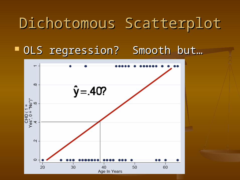
Dichotomous ScatterplotDichotomous Scatterplot

OLS regression? Smooth but…OLS regression? Smooth but…

Dichotomous ScatterplotDichotomous Scatterplot

Could break X into groups to form a more Could break X into groups to form a more continuous scale for Ycontinuous scale for Y proportion or percentage scaleproportion or percentage scale

Dichotomous ScatterplotDichotomous Scatterplot

Now, plot the categorized dataNow, plot the categorized data

Notice the “S”Shape? = sigmoid

Notice that we just shifted to acontinuous scale?

Dichotomous ScatterplotDichotomous Scatterplot

We can fit a smooth function by We can fit a smooth function by modeling the probability of success modeling the probability of success (“1”) directly(“1”) directly

Model the probabilityof a ‘1’ rather than the(0,1) data directly

Another ExampleAnother Example

QuickTime™ and aTIFF (Uncompressed) decompressor

are needed to see this picture.

Another Example (cont)Another Example (cont)

QuickTime™ and aTIFF (Uncompressed) decompressor

are needed to see this picture.

Logistic EquationLogistic Equation

E(y|x)= E(y|x)= (x) = probability that a person (x) = probability that a person with a given x-score will have a score of ‘1’ with a given x-score will have a score of ‘1’ on Yon Y

Could just expand Could just expand uu to include more to include more predictors for a multiple logistic regressionpredictors for a multiple logistic regression

(x)

eu

1 eu

u 1x

Logistic RegressionLogistic Regression

- shifts the distribution (value of x where =.5)

- reflects the steepness of the transition (slope)

Features of Logistic RegressionFeatures of Logistic Regression

Change in probability is not constant Change in probability is not constant (linear) with constant changes in X(linear) with constant changes in X

probability of a success (Y = 1) given probability of a success (Y = 1) given the predictor variable (X) is a non-the predictor variable (X) is a non-linear functionlinear function

Can rewrite the logistic equation as Can rewrite the logistic equation as an Oddsan Odds

0 1 1( )ˆ( 1| )e

ˆ(1 ( 1| )) (1 )ib b Xi

i

P Y X

P Y X

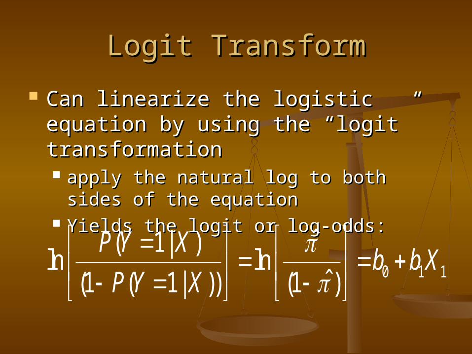
Logit TransformLogit Transform

Can linearize the logistic equation by Can linearize the logistic equation by using the “logit” transformationusing the “logit” transformation apply the natural log to both sides of the apply the natural log to both sides of the

equationequation Yields the logit or log-odds:Yields the logit or log-odds:

0 1 1

ˆ( 1| )ln ln

ˆ(1 ( 1| )) (1 )

P Y Xb b X

P Y X

Logit TransformationLogit Transformation

The logit transformation puts the The logit transformation puts the interpretation of the regression interpretation of the regression estimates back on familiar footingestimates back on familiar footing = expected value of the logit (log-= expected value of the logit (log-

odds) when X = 0odds) when X = 0 = ‘logit difference’ = The amount the = ‘logit difference’ = The amount the

logit (log-odds) changes, with a one unit logit (log-odds) changes, with a one unit change in X; change in X;

LogitLogit

LogitLogit the natural log of the oddsthe natural log of the odds often called a log odds often called a log odds logit scale is continuous, linear, and logit scale is continuous, linear, and

functions much like a z-score scale.functions much like a z-score scale. p = 0.50, then logit = 0p = 0.50, then logit = 0 p = 0.70, then logit = 0.84p = 0.70, then logit = 0.84 p = 0.30, then logit = -0.84p = 0.30, then logit = -0.84

Odds-Ratios and Logistic Odds-Ratios and Logistic RegressionRegression

The slope may also be interpreted as The slope may also be interpreted as the log odds-ratio associated with a the log odds-ratio associated with a unit increase in xunit increase in x exp(exp()=odds-ratio)=odds-ratio

Compare the log odds (logit) of a Compare the log odds (logit) of a person with a score of x to a person person with a score of x to a person with a score of x+1with a score of x+1

logit( ( ))x x logit( ( 1)) ( 1)x x x

There and back again…There and back again…

If the data are consistent with a logistic If the data are consistent with a logistic function, then the relationship between the function, then the relationship between the model and the logit is linearmodel and the logit is linear

The logit scale is somewhat difficult to The logit scale is somewhat difficult to understandunderstand

Could interpret as odds but people seem to Could interpret as odds but people seem to prefer probability as the natural scale, so…prefer probability as the natural scale, so…

log logit( )1

pp x

p

There and back again…There and back again…

log logit( )1

pp x

p

1xp

ep

Logit

1

x

x

ep

e

Odds

Probability

EstimationEstimation

Don’t meet OLS assumptions so Don’t meet OLS assumptions so some variant of MLE is usedsome variant of MLE is used

Let’s develop the likelihoodLet’s develop the likelihood

Assuming observations are Assuming observations are independent…independent…

p(yi 1) i

p(yi 0) 1 i

pdf : fi (yi ) iyi (1 i )

1 yi ; yi 0,1; i 1,2...n

joint pdf : fi (yi )i1

n

iyi (1 i )

1 yi

i1

n

EstimationEstimation

LikelihoodLikelihood

recall..recall..

joint pdf : fi (yi )i1

n

iyi (1 i )

1 yi

i1

n

log transform [yi log( i1 i

)]i1

n

log(1 i )i1

n

log i

1 i

x

1 i 1

1 exp( x)

EstimationEstimation

Upon substitution…Upon substitution…

log l l(,) yi ( x) log[1 exp( x)]i1

n

i1

n

ExampleExample

Heart Disease & AgeHeart Disease & Age 100 participants100 participants DV = presence of heart diseaseDV = presence of heart disease IV = AgeIV = Age

Heart Disease ExampleHeart Disease Example

20 30 40 50 60 70

0.0

0.2

0.4

0.6

0.8

1.0

Age

Hea

rt D

isea

se

Heart Disease ExampleHeart Disease Example

library(MASS) library(MASS) glm(formula = y ~ x, family = glm(formula = y ~ x, family =

binomial,data=mydata)binomial,data=mydata)Coefficients: Estimate Std. Error z value Pr(>|z|) (Intercept) -5.30945 1.13365 -4.683 2.82e-06 ***age 0.11092 0.02406 4.610 4.02e-06 ***

Null deviance: 136.66 on 99 degrees of freedomResidual deviance: 107.35 on 98 degrees of freedomAIC: 111.35

Number of Fisher Scoring iterations: 4

Heart Disease ExampleHeart Disease Example

Logistic regressionLogistic regression

Odds-RatioOdds-Ratio exp(.111)=1.117exp(.111)=1.117

5.31 .111( )

5.31 .111( )( )

1

x

x

ex

e

20 30 40 50 60 70

0.1

0.2

0.3

0.4

0.5

0.6

0.7

Age

p(H

eart

Dis

ease

)

Heart Disease ExampleHeart Disease Example

In terms of logits…In terms of logits…

20 30 40 50 60 70

-3-2

-10

Age

Logi

t->

(p/(

1-p)

)