Ordinal logistic regression (Cumulative logit modeling...
22
Categorical outcome variables (Beyond 0/1 data) (Chapter 6) • Ordinal logistic regression (Cumulative logit modeling) • Proportion odds assumption • Multinomial logistic regression • Independence of irrelevant alternatives, Discrete choice models Although there are some differences in terms of interpretation of parameter estimates, the essential ideas are similar to binomial logistic regression.
Transcript of Ordinal logistic regression (Cumulative logit modeling...

Categorical outcome variables (Beyond 0/1 data) (Chapter 6)
• Ordinal logistic regression (Cumulative logit modeling)
• Proportion odds assumption
• Multinomial logistic regression
• Independence of irrelevant alternatives, Discrete choice models
Although there are some differences in terms of interpretation of parameter
estimates, the essential ideas are similar to binomial logistic regression.

Ordered categorical outcomes Examples: tumor stage (local, regional, distant), disability severity (none, mild, moderate severe), Likert items (strong disagree, disagree, agree, strongly agree), weight status (underweight, normal, overweight, obese)
• Dichotomize at some fixed level corresponding to a logical outcome of interest, e.g. maybe it is particularly of interest to distinguish between tumors detected at the regional stage and those at the distant stage, hence we could dichotomize the stages at that point.
• Could treat the ordered categories as a continuous variable. If it is reasonable to assume that a unit difference between one level and the next is constant, then this can be a reasonable approach. Often Likert items are simply treated as if they are continuous scores with unit increments 1,2,3,4.
• Both above methods are suboptimal since they either throw out information (dichotomizing) or make uncheckable assumptions (treating as continuous)
• A popular way to model the ordered categories directly is using an ordered logistic regression, also called ordinal or cumulative logistic regression and also called a “proportional odds model” which aptly states the model’s main assumption
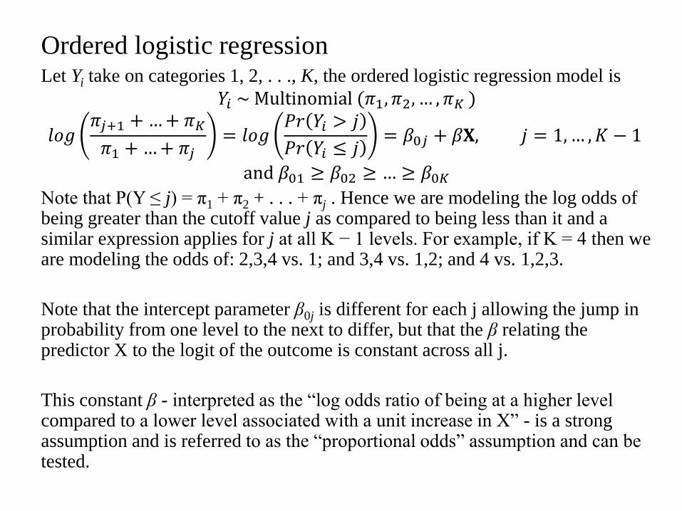
Ordered logistic regression Let Yi take on categories 1, 2, . . ., K, the ordered logistic regression model is
𝑌𝑖 ~ Multinomial (𝜋1, 𝜋2, … , 𝜋𝐾 )
𝑙𝑜𝑔𝜋𝑗+1 + … + 𝜋𝐾
𝜋1 + … + 𝜋𝑗= 𝑙𝑜𝑔
𝑃𝑟 𝑌𝑖 > 𝑗
𝑃𝑟 𝑌𝑖 ≤ 𝑗= 𝛽0𝑗 + 𝛽𝐗, 𝑗 = 1, … , 𝐾 − 1
and 𝛽01 ≥ 𝛽02 ≥ … ≥ 𝛽0𝐾
Note that P(Y ≤ j) = π1 + π2 + . . . + πj . Hence we are modeling the log odds of being greater than the cutoff value j as compared to being less than it and a similar expression applies for j at all K − 1 levels. For example, if K = 4 then we are modeling the odds of: 2,3,4 vs. 1; and 3,4 vs. 1,2; and 4 vs. 1,2,3.
Note that the intercept parameter β0j is different for each j allowing the jump in probability from one level to the next to differ, but that the β relating the predictor X to the logit of the outcome is constant across all j.
This constant β - interpreted as the “log odds ratio of being at a higher level compared to a lower level associated with a unit increase in X” - is a strong assumption and is referred to as the “proportional odds” assumption and can be tested.
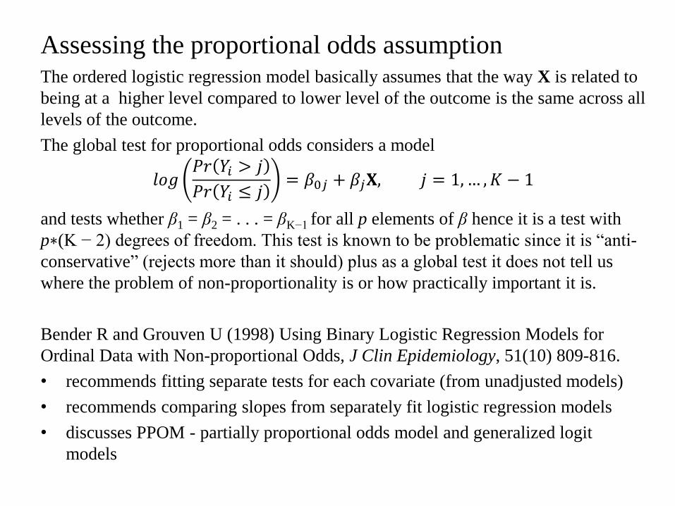
Assessing the proportional odds assumption The ordered logistic regression model basically assumes that the way X is related to
being at a higher level compared to lower level of the outcome is the same across all
levels of the outcome.
The global test for proportional odds considers a model
𝑙𝑜𝑔𝑃𝑟 𝑌𝑖 > 𝑗
𝑃𝑟 𝑌𝑖 ≤ 𝑗= 𝛽0𝑗 + 𝛽𝑗𝐗, 𝑗 = 1, … , 𝐾 − 1
and tests whether β1 = β2 = . . . = βK−1 for all p elements of β hence it is a test with
p∗(K − 2) degrees of freedom. This test is known to be problematic since it is “anti-
conservative” (rejects more than it should) plus as a global test it does not tell us
where the problem of non-proportionality is or how practically important it is.
Bender R and Grouven U (1998) Using Binary Logistic Regression Models for
Ordinal Data with Non-proportional Odds, J Clin Epidemiology, 51(10) 809-816.
• recommends fitting separate tests for each covariate (from unadjusted models)
• recommends comparing slopes from separately fit logistic regression models
• discusses PPOM - partially proportional odds model and generalized logit
models
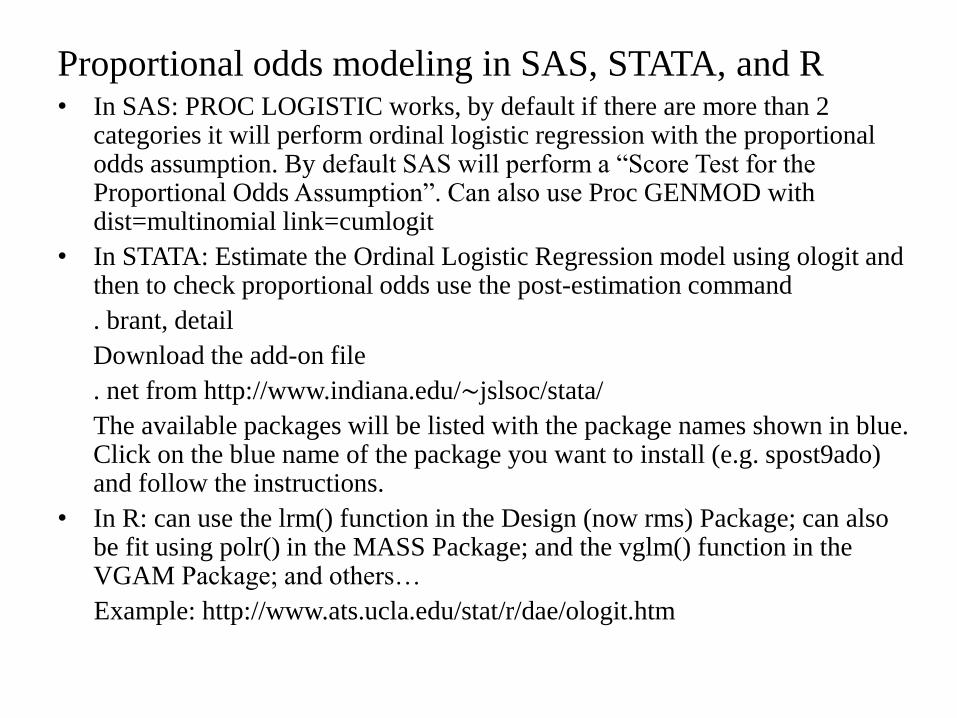
Proportional odds modeling in SAS, STATA, and R • In SAS: PROC LOGISTIC works, by default if there are more than 2
categories it will perform ordinal logistic regression with the proportional odds assumption. By default SAS will perform a “Score Test for the Proportional Odds Assumption”. Can also use Proc GENMOD with dist=multinomial link=cumlogit
• In STATA: Estimate the Ordinal Logistic Regression model using ologit and then to check proportional odds use the post-estimation command
. brant, detail
Download the add-on file
. net from http://www.indiana.edu/∼jslsoc/stata/
The available packages will be listed with the package names shown in blue. Click on the blue name of the package you want to install (e.g. spost9ado) and follow the instructions.
• In R: can use the lrm() function in the Design (now rms) Package; can also be fit using polr() in the MASS Package; and the vglm() function in the VGAM Package; and others…
Example: http://www.ats.ucla.edu/stat/r/dae/ologit.htm

Birthweight example: Stata
Mother’s baseline bmi category is regressed on age and parity.
. xi: ologit c_baseline_bmi i.parityftpt3cat age_lmp
i.parityftpt3~t _Iparityftp_0-2 (naturally coded; _Iparityftp_0 omitted)
Ordered logistic regression Number of obs = 2000
LR chi2(3) = 55.14
Prob > chi2 = 0.0000
Log likelihood = -2385.3117 Pseudo R2 = 0.0114
--------------------------------------------------------------------------------
c_baseline_bmi | Coef. Std. Err. z P>|z| [95% Conf. Interval]
---------------+----------------------------------------------------------------
_Iparityftp_1 | .1536237 .0992048 1.55 0.121 -.0408142 .3480616
_Iparityftp_2 | .663759 .1073115 6.19 0.000 .4534323 .8740857
age_lmp | .0227954 .0080193 2.84 0.004 .0070779 .0385129
---------------+----------------------------------------------------------------
/cut1 | -1.632739 .2307082 -2.084919 -1.180559
/cut2 | 1.050924 .2248569 .6102129 1.491636
/cut3 | 1.742057 .2265837 1.297961 2.186153
--------------------------------------------------------------------------------
. ologit, or <-- to show odds ratios
...

Birthweight example: Stata (test for proportional odds)
. brant, detail
Estimated coefficients from j-1 binary regressions
y>1 y>2 y>3
_Iparityftp_1 -.07919096 .15520257 .28841532
_Iparityftp_2 .245485 .70531414 .75288058
age_lmp .07588288 .01187854 .01914656
_cons .37355111 -.76029493 -1.7073335
Brant Test of Parallel Regression Assumption
Variable | chi2 p>chi2 df
-------------+--------------------------
All | 19.83 0.003 6
-------------+--------------------------
_Iparityft~1 | 4.21 0.122 2
_Iparityft~2 | 4.45 0.108 2
age_lmp | 15.05 0.001 2
----------------------------------------
A significant test statistic provides evidence that the parallel
regression assumption has been violated.
Note: -brant- is not fully compatible with newer version of Stata. Have to use -
xi- prefix for categorical variables.

Birthweight example: SAS (1)
Data Set WORK.BIRTHWGT
Response Variable c_baseline_bmi
Number of Response Levels 4
Model cumulative logit
Optimization Technique Fisher's scoring
Number of Observations Read 2000
Number of Observations Used 2000
Response Profile
Ordered c_baseline_ Total
Value bmi Frequency
1 4 582
2 3 311
3 2 945
4 1 162
Probabilities modeled are cumulated over the lower Ordered Values.

Birthweight example: SAS (2) Model Convergence Status
Convergence criterion (GCONV=1E-8) satisfied.
Score Test for the Proportional Odds Assumption
Chi-Square DF Pr > ChiSq
20.7129 6 0.0021
Model Fit Statistics
Intercept
Intercept and
Criterion Only Covariates
AIC 4831.766 4782.623
SC 4848.569 4816.229
-2 Log L 4825.766 4770.623
Testing Global Null Hypothesis: BETA=0
Test Chi-Square DF Pr > ChiSq
Likelihood Ratio 55.1429 3 <.0001
Score 54.7351 3 <.0001
Wald 54.5996 3 <.0001
Type 3 Analysis of Effects
Wald
Effect DF Chi-Square Pr > ChiSq
parityftpt3cat 2 39.0735 <.0001
age_lmp 1 8.0750 0.0045

Birthweight example: SAS (3) Analysis of Maximum Likelihood Estimates
Standard Wald
Parameter DF Estimate Error Chi-Square Pr > ChiSq
Intercept 4 1 -1.7421 0.2270 58.8952 <.0001
Intercept 3 1 -1.0509 0.2248 21.8458 <.0001
Intercept 2 1 1.6327 0.2306 50.1474 <.0001
parityftpt3cat 1 1 0.1536 0.0988 2.4153 0.1202
parityftpt3cat 2 1 0.6638 0.1072 38.3319 <.0001
age_lmp 1 0.0228 0.00802 8.0750 0.0045
Odds Ratio Estimates
Point 95% Wald
Effect Estimate Confidence Limits
parityftpt3cat 1 vs 0 1.166 0.961 1.415
parityftpt3cat 2 vs 0 1.942 1.574 2.396
age_lmp 1.023 1.007 1.039
Note: the estimated intercepts in SAS has opposite sign as in Stata. See next
slide for details.

Backtransforming to probabilities
In SAS -- logit(Pr(Y_i >= j)) = alpha_j + beta*X
In Stata -- logit(Pr(Y_i <= j)) = alpha_j - beta*X
EXAMPLE: For parity3cat = 0 and age_lmp = 25, we have:
IN SAS:
-1.7421 + 25*.0228 = -1.1721 --> invlogit(-1.1721) = Prob(4) = .236
-1.0509 + 25*.0228 = 0.04809 --> invlogit(.04809) = Prob(3 or 4) = .512
1.637 + 25*.0228 = 2.207 --> invlogit(2.207) = Prob(2,3, or 4) = .901
In Stata:
1.7421 - 25*.0228 = 1.1721 --> invlogit(1.1721) = Prob(1,2 or 3) = 1-.236=.763
1.0509 - 25*.0228 = -0.04809 --> invlogit(-.04809) = Prob(1 or 2) = 1-.512=.488
-1.637 - 25*.0228 = -2.207 --> invlogit(-2.207) = Prob(1) = 1-.901 = .099
So for a woman who has not had any previous kids (parity3cat = 0) and is 25
years old when she gets pregnant, her predicted probability of being obese at
the time she gets pregnant is 0.236. What is her probability of being of Normal
weight (2)?

Outcome: nominal categories
Examples: consumer brand choice (Geico, State Farm, Acuity, Progressive),
homeless sleeping situation (on street, with friend/family, hotel, shelter),
parenting style (authorative, authoritarian, permissive, neglectful)
• Could run separate logistic regression models, one comparing each pair of
outcomes. In fact this is quite similar to what the multinomial logistic
regression model does, but it is slightly less efficient and can only produce
dichotomous predicted probabilities (rather than probability of being in any
of the K categories), also does not allow for an overall test of covariate
related to differences across any category. Advantage of separate logistic
regressions is ease of interpretation.
• Could collapse categories so there were only two and then do a logistic
regression, but this would lose information that may be of interest across
categories
• Multinomial logistic or “generalized logit” models are a way to fit a
nominal category outcome in a regression framework.
• Can also use when the POM assumption does not apply to an ordinal
outcome
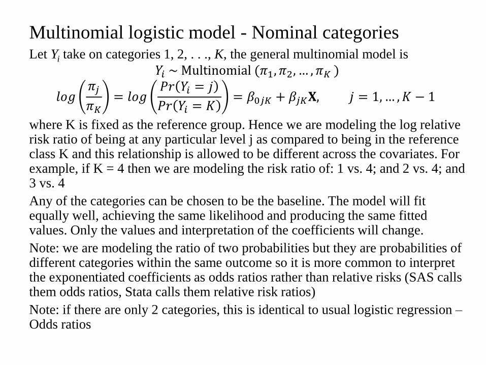
Multinomial logistic model - Nominal categories Let Yi take on categories 1, 2, . . ., K, the general multinomial model is
𝑌𝑖 ~ Multinomial (𝜋1, 𝜋2, … , 𝜋𝐾 )
𝑙𝑜𝑔𝜋𝑗
𝜋𝐾= 𝑙𝑜𝑔
𝑃𝑟 𝑌𝑖 = 𝑗
𝑃𝑟 𝑌𝑖 = 𝐾= 𝛽0𝑗𝐾 + 𝛽𝑗𝐾𝐗, 𝑗 = 1, … , 𝐾 − 1
where K is fixed as the reference group. Hence we are modeling the log relative risk ratio of being at any particular level j as compared to being in the reference class K and this relationship is allowed to be different across the covariates. For example, if K = 4 then we are modeling the risk ratio of: 1 vs. 4; and 2 vs. 4; and 3 vs. 4
Any of the categories can be chosen to be the baseline. The model will fit equally well, achieving the same likelihood and producing the same fitted values. Only the values and interpretation of the coefficients will change.
Note: we are modeling the ratio of two probabilities but they are probabilities of different categories within the same outcome so it is more common to interpret the exponentiated coefficients as odds ratios rather than relative risks (SAS calls them odds ratios, Stata calls them relative risk ratios)
Note: if there are only 2 categories, this is identical to usual logistic regression – Odds ratios

Multinomial logistic model in SAS, STATA, and R
• In SAS: use PROC LOGISTIC and add the /link=glogit option on the model
statement. Can fix the reference class of the outcome variable (i.e. what is K)
by adding (ref = ’name’) after the outcome in the model statement.
• In Stata: use -mlogit- command. Can fix the reference by using the
baseoutcome () option. Can get exponentiated coefficients by using the rrr
option.
• In R: use multinom() in the nnet library of the MASS package, or vglm() in
the VGAM package.
Example: http://www.ats.ucla.edu/stat/r/dae/mlogit.htm

Independence of irrelevant alternatives
In multinomial logistic regression, it is assumed that adding or removing
categories does not affect the odds associated with the remaining categories.
This is called Independence of irrelevant alternatives (IIA).
Humorous example of violation of the IIA assumption from a Groucho Marx
sketch:
Marx was dining in a posh restaurant when the waiter informed him that the
specials for the evening were steak, fish and chicken. Groucho ordered the
steak. The waiter returned later and apologized that there was no fish that
evening. Groucho replied, “In that case, I’ll have the chicken”. (example
taken from Hardin and Hilbe Generalized Linear Models and Extensions
(2007))
There are statistical tests to check for IIA assumption, but they all perform
poorly. The general advice is to use multinomial logistic model when you can
clearly distinguish between the outcome categories in your dataset.
When the IIA assumption is violated, alternative-specific multinomial probit
regression is recommended which allows for dependence across the categories.
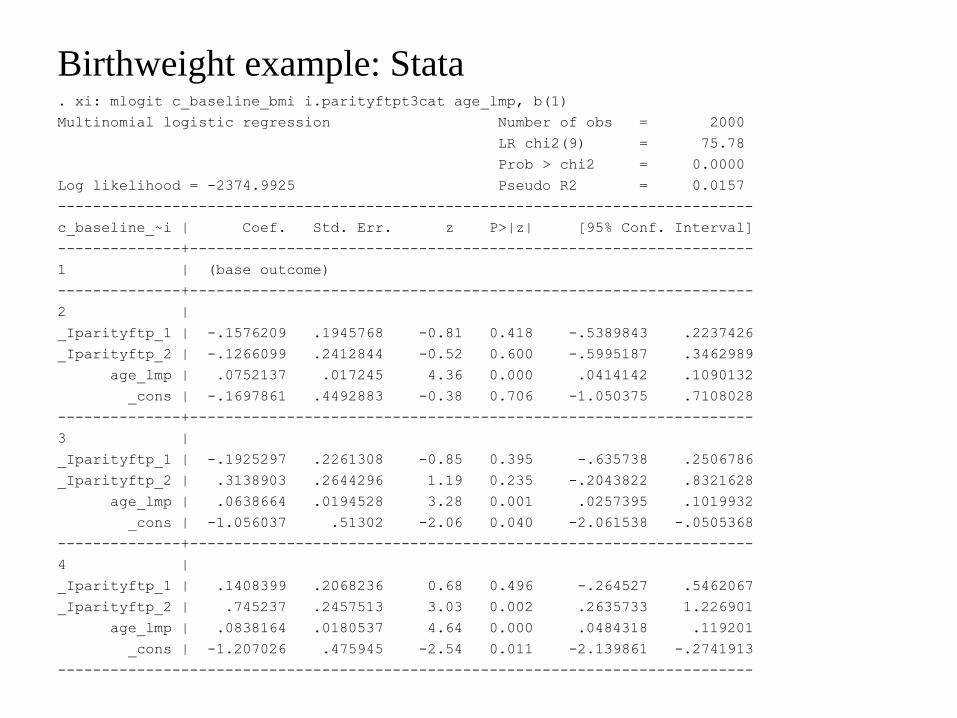
Birthweight example: Stata . xi: mlogit c_baseline_bmi i.parityftpt3cat age_lmp, b(1)
Multinomial logistic regression Number of obs = 2000
LR chi2(9) = 75.78
Prob > chi2 = 0.0000
Log likelihood = -2374.9925 Pseudo R2 = 0.0157
-------------------------------------------------------------------------------
c_baseline_~i | Coef. Std. Err. z P>|z| [95% Conf. Interval]
--------------+----------------------------------------------------------------
1 | (base outcome)
--------------+----------------------------------------------------------------
2 |
_Iparityftp_1 | -.1576209 .1945768 -0.81 0.418 -.5389843 .2237426
_Iparityftp_2 | -.1266099 .2412844 -0.52 0.600 -.5995187 .3462989
age_lmp | .0752137 .017245 4.36 0.000 .0414142 .1090132
_cons | -.1697861 .4492883 -0.38 0.706 -1.050375 .7108028
--------------+----------------------------------------------------------------
3 |
_Iparityftp_1 | -.1925297 .2261308 -0.85 0.395 -.635738 .2506786
_Iparityftp_2 | .3138903 .2644296 1.19 0.235 -.2043822 .8321628
age_lmp | .0638664 .0194528 3.28 0.001 .0257395 .1019932
_cons | -1.056037 .51302 -2.06 0.040 -2.061538 -.0505368
--------------+----------------------------------------------------------------
4 |
_Iparityftp_1 | .1408399 .2068236 0.68 0.496 -.264527 .5462067
_Iparityftp_2 | .745237 .2457513 3.03 0.002 .2635733 1.226901
age_lmp | .0838164 .0180537 4.64 0.000 .0484318 .119201
_cons | -1.207026 .475945 -2.54 0.011 -2.139861 -.2741913
-------------------------------------------------------------------------------

Birthweight example: SAS (1) proc logistic data = birthwgt descending;
class parityftpt3cat (ref = "0") /param = ref;
model c_baseline_bmi = parityftpt3cat age_lmp/link=glogit;
run;
Model Fit Statistics
Intercept
Intercept and
Criterion Only Covariates
AIC 4831.766 4773.985
SC 4848.569 4841.196
-2 Log L 4825.766 4749.985
Testing Global Null Hypothesis: BETA=0
Test Chi-Square DF Pr > ChiSq
Likelihood Ratio 75.7813 9 <.0001
Score 75.4875 9 <.0001
Wald 73.7188 9 <.0001
Type 3 Analysis of Effects
Wald
Effect DF Chi-Square Pr > ChiSq
parityftpt3cat 6 45.3792 <.0001
age_lmp 3 22.7799 <.0001

Birthweight example: SAS (2) Analysis of Maximum Likelihood Estimates
c_baseline_ Standard Wald
Parameter bmi DF Estimate Error Chi-Square Pr > ChiSq
Intercept 4 1 -1.2070 0.4759 6.4316 0.0112
Intercept 3 1 -1.0560 0.5130 4.2373 0.0395
Intercept 2 1 -0.1698 0.4493 0.1428 0.7055
parityftpt3cat 1 4 1 0.1408 0.2068 0.4637 0.4959
parityftpt3cat 1 3 1 -0.1925 0.2261 0.7249 0.3945
parityftpt3cat 1 2 1 -0.1576 0.1946 0.6562 0.4179
parityftpt3cat 2 4 1 0.7452 0.2458 9.1960 0.0024
parityftpt3cat 2 3 1 0.3139 0.2644 1.4091 0.2352
parityftpt3cat 2 2 1 -0.1266 0.2413 0.2753 0.5998
age_lmp 4 1 0.0838 0.0181 21.5537 <.0001
age_lmp 3 1 0.0639 0.0195 10.7789 0.0010
age_lmp 2 1 0.0752 0.0172 19.0224 <.0001
Odds Ratio Estimates
c_baseline_ Point 95% Wald
Effect bmi Estimate Confidence Limits
parityftpt3cat 1 vs 0 4 1.151 0.768 1.727
parityftpt3cat 1 vs 0 3 0.825 0.530 1.285
parityftpt3cat 1 vs 0 2 0.854 0.583 1.251
parityftpt3cat 2 vs 0 4 2.107 1.302 3.411
parityftpt3cat 2 vs 0 3 1.369 0.815 2.298
parityftpt3cat 2 vs 0 2 0.881 0.549 1.414
age_lmp 4 1.087 1.050 1.127
age_lmp 3 1.066 1.026 1.107
age_lmp 2 1.078 1.042 1.115

Multinomial Discrete Choice models
Choice-specific vs. case-specific independent variables. Where the dependent is
a choice among alternatives, choice-specific independent variables vary both
across choices and across cases. Case-specific variables, in contrast, vary only
across cases but are uniform within any choice category.
An dining choice (nested logit) example from Stata manual:
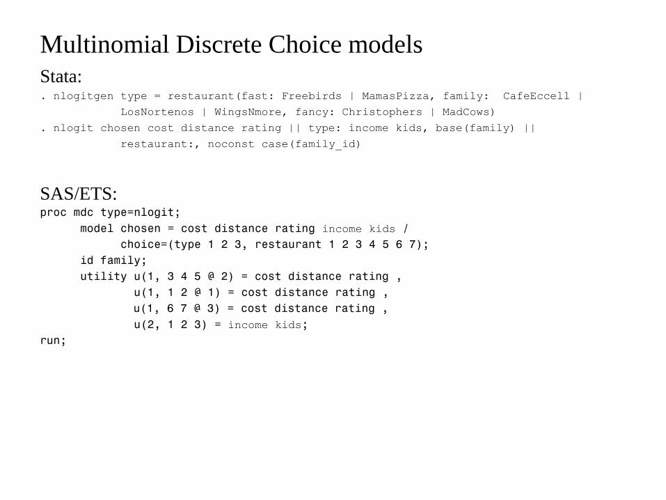
Multinomial Discrete Choice models
Stata: . nlogitgen type = restaurant(fast: Freebirds | MamasPizza, family: CafeEccell |
LosNortenos | WingsNmore, fancy: Christophers | MadCows)
. nlogit chosen cost distance rating || type: income kids, base(family) ||
restaurant:, noconst case(family_id)
SAS/ETS: proc mdc type=nlogit;
model chosen = cost distance rating income kids /
choice=(type 1 2 3, restaurant 1 2 3 4 5 6 7);
id family;
utility u(1, 3 4 5 @ 2) = cost distance rating ,
u(1, 1 2 @ 1) = cost distance rating ,
u(1, 6 7 @ 3) = cost distance rating ,
u(2, 1 2 3) = income kids;
run;

Review
Generalized Linear Models
• Binary outcome
– Relation between odds ratios, relative risks, risk differences. How to
estimate them using different link functions (logit, log, identity).
– Calculating predicted probabilities from fitted models
– Interpret and test regression coefficients or odds ratios
– Problem of separation
– Model fit: classification table, ROC curve, Hosmer Lemeshow test
• count outcomes
– Poisson regression
– The offset term (why & when to use?)
– Interpretation of coefficients
– Under and over-dispersion: definition, problem, estimation
– Residual analysis, outlier detection
Review
• Categorical outcome
– Ordinal logistic regression
• Proportional odds assumption
• Interpretation of coefficients
• Predicted probabilities
– Multinomial logistic regression
• IIA assumption
• Interpretation of coefficients