1

Localization in Wireless Sensor Networks Using Quadratic

Optimization

Pouya Mollaebrahim Gharia, Reza Shahbazian

a, Seyed Ali Ghorashi

a,b

a Cognitive Telecommunication Research Group, Department of Electrical Engineering, Shahid Beheshti University, Tehran, Iran b Cyber Research Centre, Shahid Beheshti University, Tehran, Iran

p.molaebrahim@mail.sbu.ac.ir, r_shahbazian@sbu.ac.ir and a_ghorashi@sbu.ac.ir

Abstract The localization problem in a wireless sensor network is to determine the coordination

of sensor nodes using the known positions of some nodes (called anchors) and corresponding noisy

distance measurements. There is a variety of different approaches to solve this problem such as semi-

definite programming (SDP) based, sum of squares and second order cone programming, and between

them, SDP-based approaches have shown good performance. In recent years, the primary SDP approach

has been investigated and a variety of approaches are proposed in order to enhance its performance. In

SDP approaches, errors in approximating the given distances are minimized as an objective function. It is

desirable that the distribution of error in these problems would be a delta distribution, which is practically

impossible. Therefore, we may approximate delta distribution by Gaussian distribution with very small

variance. In this paper, we define a new objective function which makes the error distribution as similar

as possible to a Gaussian distribution with a very small variance. Simulation results show that our

proposed method has higher accuracy compared to the traditional SDP approach and other prevalent

objective functions which are used such as least squares. Our method is also faster than other popular

approaches which try to improve the accuracy of the primary SDP approach.

Keywords: Localization, Wireless sensor network, Semi-definite programming (SDP).

1. Introduction

A sensor network may contain a large set of inexpensive and autonomous sensor nodes that can

communicate with their neighbors within a limited radio range. Today, sensor networks have a wide

variety of applications in diverse areas such as wildlife monitoring, industrial control and monitoring [1],

robotics [2] and medical applications [3]. Determination of the exact location of sensors is a necessity in

many of these applications.

One approach to solve this problem is using GPS (Global Positioning System). However, this

could be expensive and it may not work very well in some areas [4, 7]. Alternatively, the known

locations of some nodes (called anchors) and the distance measurements among neighbor sensors [4, 8,

10] can be used to localize the sensors. In this method, distance measurements are usually corrupted by

noise, which may cause errors in target location estimation. In order to minimize this error, sensor

network localization can be viewed as an optimization problem, and although it is not convex, some

relaxation methods are proposed in the literature to solve this problem.

One of the first proposed convex optimization models for wireless sensor network (WSN)

localization is introduced in [11] in which the problem is relaxed to a second order cone programming

(SOCP) problem. However, this method needs a large number of anchors on the area boundary to show

effective performance as reported in [1]. In [5] the authors introduce a semi-definite programming (SDP)

relaxation method for WSN localization, and they report that their proposed method outperforms the

method in [11] in terms of accuracy. However, some localization errors happen with rather high

variances in this method. In [6], two formulations are developed to deal with noisy corrupted data, and

SDP relaxation is used to transform the problem into a convex optimization problem; the first approach is

based on maximum likelihood (ML) estimation and the second one is based on solving an SDP feasibility

2

problem with upper and lower bound distance measures [6]. However, ML based methods are very time

consuming in comparison with other proposed methods.

The authors in [12] propose a method called smaller SDP (SSDP) to further relax the SDP

relaxation. In this method, they relax a single semi-definite matrix cone into a set of small-size semi-

definite matrix cones. The two relaxations are proposed in [12] include a node-based relaxation (called

NSDP) and an edge-based relaxation named ESDP. Although these proposed relaxations are weaker than

the original SDP one, the SSDP is faster compared to others. To find a low rank solution for this problem

is investigated in [13] in which a non-convex objective function is proposed. However, the use of this

objective function failed to provide more accuracy compared to traditional SDP models. Authors in [2]

propose a convex relaxation to solve the localization problem based on maximum likelihood (ML)

formulation. The convex relaxation is similar to the SSDP. In [14] the sum of squares (SOS) convex

relaxation method is proposed which is very accurate, but it is at the cost of high computation

complexity. In [15], authors attempt to address the non-convexity of the problem by introducing a convex

objective function but this method is only effective for noise-free measurement cases.

Minimizing the sum of absolute errors as an objective function in the optimization problem may

cause large errors [5], and this affects the accuracy of the localization process (this will be shown in

section 4). In this paper, we propose a multi-criterion optimization method in WSN localization to reach

greater accuracy with not much computational complexity compared to those methods mentioned earlier.

Our proposed objective function makes the distribution of error close to Gaussian distribution with a very

small variance. This is an approximation of desirable delta distribution for estimation error and therefore

the proportion of large errors is effectively reduced.

The remainder of this paper is organized as follows. Section 2 explains the problem formulation.

In section 3 the proposed convex relaxations are introduced. The numerical results of the proposed

technique and its performance comparisons are presented in section 4, and finally section 5 concludes the

paper.

2. Problem Formulation

In this section we present the Biswas-Ye model for WSN localization. In this method, the

problem is relaxed to a SDP model. We use ,ie and 0 to denote the identity matrix, zero column vector

except for 1 in position i and the vector of all zeros, respectively. The 2-norm of a vector x denoted as x .

Also a positive semi-definite matrix X is represented by 0X . For the sake of simplicity, let the sensor

points be placed on a plane. The generalization of this problem for higher dimensions is straightforward.

Assume that there are points with known locations (anchors) 2 , 1, ,ka k m and n unknown points

(sensors) 2 , 1, ,ix i n . ˆijd is the distance measurement between two sensors

ix and jx , and ˆkjd is the

distance measurement between some sensor jx and anchor ka .

22ˆ , ( , )j i ij sx x d j i N

22ˆ , ( , )j k jk ax a d j k N

wheresN and

aN are the set of pairs ( , )j i in which the sensors  i and j are connected and the set of pairs  ( , )j k

in which the sensor j is connected to anchor k, respectively. Nodes ( , ) si j N (or ( , ) aj k N ) are called

connected if the associated measurements ˆijd (or ˆ

kjd ) do exist for sensor/anchor pairs. Then, the

localization problem is to find the location of n sensors by means of given m anchor locations and some

distance measurements. We consider a two dimensional localization and then extension to three

dimensional is straight forward. Hence, the localization problem can be written as follows: 2 ,n n nfind X Y (1)

2ˆ. . , ( , )T

i j i j ij ss t e e Y e e d j i N

3

2 2ˆ , ( , )

T

k k

jk aTj j

a aI Xd j k N

e eX Y

where I2 is a 2 by 2 identity matrix, matrix 1  , , nX x x , TY X X . The problem (1) is non-convex and may

relaxed by substituting the constraint TY X X into TY X X . This matrix inequality is equivalent to [19]:

20

TZ

I X

X Y

(2)

We define: 1

1 0 1 , 1

0 0 1 2

I IA b

0 0 0

(3)

where 0 in IA is a zero column vector of dimension n and by introducing slack variables and [5],

the problem in Eq. (1) can be written as an standard SDP problem:

( , ) ( , )

min ( ) ( )s a

ij ij jk jk

j i N j k N

(4)

. . T

I I Is t diag A ZA b

2ˆ , ( , )

T

i j i j

ij ij ij s

e e e eZ d j i N

0 0

2ˆ , ( , )

T

i i

jk jk jk a

k k

e eZ d j k N

a a

2 , ( , )

T

i j i j

ij s

e e e eZ r j i N

0 0

2 , ( , ))

T

i i

jk a

k k

e eZ r j k N

a a

0Z

, , , 0ij ij jk jk

, 1, , , 1, ,for i j n k m

where ijr or   jkr is the radio range in which the associated nodes can communicate. Biswas and Ye [5]

neglect the inequalities involving ijr and   jkr in order to reduce the problem size; it is shown in [1] that the

resulting problem is likely to satisfy most of neglected constraints.

3. Proposed quadratic programming approach

In [5] the objective function which is used in the localization problem is the l1-norm of the

squared distance error. The authors of [9] reported that if the least-squares penalty function is picked as an

objective function, more accuracy than using l1-norm can be achieved. On one hand, it is known that the

least-squares objective function put small weights on small squared-distance errors [16]. Therefore, the

localization model is comparatively sensitive to large squared-distance errors and reducing the number of

large squared-distance errors can improve the performance of the model in average. On the other hand, it

is ideal that the squared-distance error has a delta shaped PDF (probability density function) which is

impractical. In this paper, we aim to introduce a new objective function which tries to estimate the

squared-distance error’s PDF as a Gaussian distribution with a small variance, in order to avoid large

squared-distance errors and simultaneously maintain proportionally small amounts of squared-distance

errors. To start, we consider the following theorem [17]:

Theorem 1.For any random variable X and its estimate X̂ ,

2 2 ( )1ˆ( )2

h XE X X ee

(5)

where ( )h X is the differential entropy of random variable X and X̂ is the mean value of X . Equality

happens in Eq. (5) if and only if X is Gaussian.

4

Theorem 1 states that the variance of desirable estimation is zero and it is a delta function. It is

impossible to have no estimation error in practical scenarios. Therefore, we reduce the variance of the

estimation error which is more likely to reduce the relative entropy between the PDF of squared-distance

errors and Gaussian distribution. Since the Gaussian distribution is characterized by its first and second

statistics, we aim to approximate these statistics in order to make error distribution close to Gaussian

distribution with as small a standard deviation as possible. Thus, involving the variance of squared-

distance error in the optimization problem can reduce the difference between the distribution of squared-

distance error and Gaussian distribution with a small standard deviation.

As mentioned earlier in section 1, we consider two criteria for optimization in order to obtain

higher accuracy. The first criterion is the mean of the squared-distance errors i.e. ij ij and jk jk .

Obviously, we aim to minimize this criterion in order to make the mean of squared-distance errors as

close as possible to the mean of associated Gaussian distribution which is zero. The second criterion is the

variance of the squared-distance errors, in order to make the PDF of the squared distance errors as close

as possible to delta distribution. The delta distribution is approximated by Gaussian distribution and we

consider the variance of squared-distance errors as a second criterion for the optimization.

By interpreting the localization problem as a bi-criterion optimization, we have to minimize a

vector0f , which consists of two scalar functions

1F and 2F where

1F is the mean and 2F is the variance of

the squared distance error as follows:

1

, ,

1

s a

ij ij jk jk

j i N j k N

Fv

(6)

2 2

2 1 1

, ,

1( ( ) ( ) )

s a

ij ij jk jk

j i N j k N

F F Fv

(7)

where v is the number of distances between connected nodes. The objective function f0 must be

transformed into a scalar one by vector (   0 ) in a way that the optimization problem can be solved.

Therefore, we may write the objective function as:

1 2F F (8)

This objective function is non-convex. Therefore, we relax it to a convex form as follows:

2 2

1 1

, ,

1( ) 2

2 4as sa

ij ij ij ij

j i N j i NN N

vF vF

(9)

Assume that v is a vector with components of ij ij where ( , ) s ai j N N . Then, we

approximate 1F by constant m that satisfies the following constraints. Let l be a constant value which

satisfies the following:

, ,

1 1

s sa a

ij

N N

ij

j i N j i N

mv v

(10)

11m m

v (11)

,

1

s a

ij

j i N N

mv

(12)

2 2

1F m l

We relax the objective function by using the Jensen’s inequality and write the relaxed objective function

as follows:

22

2

2

,

1 1

2 4as

ij

j i N N

m v v lv v

(13)

In Eq. (13) we have substituted ,

1

s a

ij

j N Niv

with1F . Since the objective function is positive, this tightening

preserves convexity. Now we can conclude that:

2 2 2 2 211 1 0 ( ) 0m m m v vm v m v m v m

v (14)

5

If γ satisfies the constraint γ 1 2m along with other constraints in the problem, we prove that the

relaxed objective function is an upper bound of the non-convex objective function. Knowing the convex

upper bound, we may solve the optimization problem. Therefore we have:

2 2 2 2 2 2

, ,

2 1 ( ) 0

sas a

ij ij ij

j i NN j i N N

m v m v m v m v

(15)

We may write the following statement:

22

2

1 22

,

112 4

s aN

ij

j i N

m v v l F Fv v

(16)

After eliminating constant terms and relaxing the objective function, we can write the objective function

as follows:

22

,

12

as

ij

j i NN

v

(17)

We take as ,

2

s aijj N Ni

v

in Eq. (17) to satisfy all the constraints, therefore:

2 2

, ,

1

s sa aN

ij ij

j N Ni j i N

vv

(18)

Since the regularization coefficient γ must be positive and in order to guarantee that the relaxed objective

function is the upper bound of the original objective function, we have to add the following constraint in

the SDP model:

,

0

as

ij

j i N N

(19)

On one hand, adding Eq. (19) as a constraint in the optimization model increases the problem

size. On the other hand, the resulting model with neglecting this constraint is likely to satisfy both

positive γ and the objective function upper bound. Therefore, we may neglect this constraint.

It is straight forward to prove that the function in Eq. (18) is convex. Using the relaxation Biswas and Ye

[5] applied for sensor network localization, we may write the optimization problem as Eq. (20) where ( )w mean in the following model:

1 2minvt t (20)

. . T

I I Is t diag A ZA b

2ˆ , ( , )

T

i j i j

ij ij ij s

e e e eZ d j i N

0 0

2ˆ , ( , )

T

i i

jk jk jk a

k k

e eZ d j k N

a a

1w s

2vw s

1

1 1

10

s

s t

(20.a)

2

2 2

10

s

s t

(20.b)

0Z

, , , 0ij ij jk jk

, 1, , , 1, ,for i j n k m

Eq. (20.a) and Eq. (20.b) are the SOC constraints that are equivalent to quadratic constraints.

4. Simulation Results

In this section, we display the simulation results and compare our proposed quadratic

programming (QP) with other models. We use MATLAB R2010b and also SDPT3 solver in CVX

software [18] in order to solve the problems. The CPU time which is taken for localizing is extracted from

6

cvx_cputime [18]. We consider 2-dimentional problems and use the benchmark test10-500 which is

available online at http://www.stanford.edu/~yyye. The position error for sensor is defined as ˆi ix x

where ix is the true position for sensor i and ˆ

ix is the estimated location for this sensor. PE shows the

position error for the evaluated network and is defined as:

1

1ˆ

n

i

i

iPE x xn

At first we seek to find appropriate regularization coefficient in terms of position error and survey the

effect of our proposed QP model on relative entropy.

4.1. Regularization Coefficient

The section mentions the evaluation results of the regularization coefficient effect on the position

error. We consider networks which include 80 sensors and 5 anchors. The distance measurements are

corrupted by an additive Gaussian noise with standard deviation of 0.05 and radio range is set to 0.25.

The experiments are performed over 50 networks. As depicted in Fig. 1, when the regularization

coefficient becomes larger, the average position error converges to a limit. As can be seen in Fig. 1, if the

regularization coefficient is large enough, the variation of it doesn't cause a rapid change in average

position error. Therefore, we can solve the problem regardless of regularization coefficient as long as the

regularization coefficient is large enough. We try to approximate this specific amount.

Fig. 1. Average of position error as a function of regularization coefficient variations.

4.2. Relative Entropy

Relative entropy is the criterion that measures the difference between two distributions p, q and

is defined as follows:

( )

( | | ) log( )x

p xD p q p x

q x

In this section, we want to prove that our model reduces the relative entropy between distribution

of squared-distance error and Gaussian distribution. We quantize the probability distribution of squared-

distance error and divide real numbers into intervals I0, I1, ... with a specific length and then calculate the

probability associated to interval , {0,1, }iI i as follow:

i iI Ip v v

where iIv is the number of squared-distance errors lie in

iI and v is the total number of squared-distance

errors.

Now, we study the effect of our proposed QP approach on the amount of mentioned relative

entropy. We set the length of intervals to 0.0049 and choose 0.008 as the standard deviation of Gaussian

distribution. Networks consist of 80 sensors and 5 anchors. The distance measurements between

connected nodes are corrupted by additive Gaussian noise with standard deviation 0.05 and similar to

prior experiment, the radio range is set to 0.25. We use 50 networks for operating the experiment.

10-1

100

101

102

103

104

0.179

0.18

0.181

0.182

0.183

0.184

0.185

0.186

0.187

0.188

regulariaztion coefficient

avera

ge p

ositio

n e

rror

7

The relative entropy is measured for the proposed QP, Biswas-Ye and LS. The average of results

are depicted in Table 1 and show that our proposed QP approach reduces the relative entropy dramatically

in comparison with the approach in [5] and it has also a lower relative entropy in comparison with LS.

Table 1 . Relative entropy of squared-distance errors in bits for Biswas-Ye [5], LS [9] and our proposed QP.

Approach Relative

entropy (bits)

Biswas-Ye [5] 1.1232

LS [9] 0.2229

Proposed QP 0.2089

Figs. 2,3,4 depict the distribution of squared-distance errors for Biswas-Ye, LS and our proposed

QP approaches, respectively for one of the 50 simulated networks and illustrate that the distribution of

squared-distance errors for proposed QP is more similar to Gaussian distribution. The proportion of

squared-distance errors in the interval [0.00245, 0.0073) for the proposed QP is 0.3598 and for LS is

0.3482. The proportion of squared-distance errors in the interval [-0.00245, 0.00245) is 0.2244 for both

methods in this case. These results along with comparisons of Fig. 3 and Fig. 4 show that the density of

squared distance error in the vicinity of 0 in proposed QP is more than what in LS. As can be seen in Figs.

2, 3 and 4 the density of large squared-distance errors in Biswas-Ye is more than two other approaches.

For more illustration consider one of the simulated networks. The proportion of squared-distance errors

which are larger than 0.022 for Biswas-Ye approach is 0.0658, for LS is 0.0271 and in our proposed QP is

0.0348. In addition the maximum amount of squared distance error in Biswas-Ye approach is more than

LS and our QP model. Large squared-distance errors can degrade the performance of localization

effectively.

Fig.2. Distribution of squared-distance errors in Biswas-Ye approach [5].

-0.08 -0.06 -0.04 -0.02 0 0.02 0.04 0.06 0.080

0.1

0.2

0.3

0.4

0.5

8

Fig.3. Distribution of squared-distance errors in LS approach [9].

Fig.4. Distribution of squared-distance errors in proposed QP approach.

4.3. Noise Standard Deviation

In this section, we consider the performance of our proposed QP approach in comparison with

Biswas-Ye, EML, ML and LS by increasing the noise value. We evaluate our proposed method and other

introduced methods over 50 networks. As depicted in Fig. 5, the performance of our proposed QP shows

higher accuracy in comparison with Biswas-Ye, LS and EML in all noise standard deviation intervals. As

can be seen in Fig. 5, when the standard deviation of noise becomes larger, the difference between the

accuracy of proposed QP and ML reduces. However, as will be shown in 4.5 our QP method has lower

complexity in comparison with ML.

Fig.5. Performance comparison between the approaches for various standard deviations of noise.

-0.06 -0.04 -0.02 0 0.02 0.04 0.060

0.05

0.1

0.15

0.2

-0.06 -0.04 -0.02 0 0.02 0.04 0.060

0.05

0.1

0.15

0.2

0.01 0.02 0.03 0.04 0.05 0.06 0.07 0.08 0.09 0.1 0.110.06

0.08

0.1

0.12

0.14

0.16

0.18

0.2

0.22

0.24

the standard deviation of noise

avera

ge p

ositio

n e

rror

Biswas-Ye[5]

EML[2]

ML[6]

LS[9]

proposed QP

9

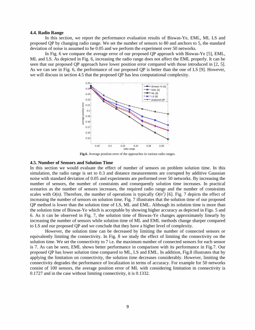
4.4. Radio Range

In this section, we report the performance evaluation results of Biswas-Ye, EML, ML LS and

proposed QP by changing radio range. We set the number of sensors to 80 and anchors to 5, the standard

deviation of noise is assumed to be 0.05 and we perform the experiment over 50 networks.

In Fig. 6 we compare the average error of our proposed QP approach with Biswas-Ye [5], EML,

ML and LS. As depicted in Fig. 6, increasing the radio range does not affect the EML properly. It can be

seen that our proposed QP approach have lower position error compared with those introduced in [2, 5].

As we can see in Fig. 6, the performance of our proposed QP is better than the one of LS [9]. However,

we will discuss in section 4.5 that the proposed QP has less computational complexity.

Fig.6. Average position error of the approaches in various radio ranges.

4.5. Number of Sensors and Solution Time

In this section we would evaluate the effect of number of sensors on problem solution time. In this

simulation, the radio range is set to 0.3 and distance measurements are corrupted by additive Gaussian

noise with standard deviation of 0.05 and experiments are performed over 50 networks. By increasing the

number of sensors, the number of constraints and consequently solution time increases. In practical

scenarios as the number of sensors increases, the required radio range and the number of constraints

scales with O(n). Therefore, the number of operations is typically O(n3) [6]. Fig. 7 depicts the effect of

increasing the number of sensors on solution time. Fig. 7 illustrates that the solution time of our proposed

QP method is lower than the solution time of LS, ML and EML. Although its solution time is more than

the solution time of Biswas-Ye which is acceptable by showing higher accuracy as depicted in Figs. 5 and

6. As it can be observed in Fig. 7, the solution time of Biswas-Ye changes approximately linearly by

increasing the number of sensors while solution time of ML and EML methods change sharper compared

to LS and our proposed QP and we conclude that they have a higher level of complexity.

However, the solution time can be decreased by limiting the number of connected sensors or

equivalently limiting the connectivity. In Fig. 8 we study the effect of limiting the connectivity on the

solution time. We set the connectivity to 7 i.e. the maximum number of connected sensors for each sensor

is 7. As can be seen, EML shows better performance in comparison with its performance in Fig.7. Our

proposed QP has lower solution time compared to ML, LS and EML. In addition, Fig.8 illustrates that by

applying the limitation on connectivity, the solution time decreases considerably. However, limiting the

connectivity degrades the performance of localization in terms of accuracy. For example for 50 networks

consist of 100 sensors, the average position error of ML with considering limitation in connectivity is

0.1727 and in the case without limiting connectivity, it is 0.1332.

0.18 0.2 0.22 0.24 0.26 0.28

0.15

0.16

0.17

0.18

0.19

0.2

0.21

0.22

0.23

0.24

0.25

radio range

avera

ge p

ositio

n e

rror

Biswas-Ye [5]

EML [2]

ML [6]

LS [9]

proposed QP

10

Fig.7. The effect of number of sensors on solution time (sec).

Fig.8. The effect of number of sensors on solution time (sec) with limiting the connectivity to 7.

Fig. 9 depicts the coordinates of sensor's location estimation for Biswas-Ye, EML, ML, LS and

proposed QP approach along with exact locations. The network consists of 20 sensors and 5 anchors,

radio range is fixed to 0.4 and the standard deviation of additive Gaussian noise is 0.01. As can be seen in

Fig. 9, EML has worst performance among all other approaches, LS and proposed QP has the same

performance in most cases.

Fig.9. The coordinates which localize with Biswas-Ye [5], EML[2], ML[6], LS[9] and proposed QP along with their exact locations.

5. Conclusion

In this paper we consider the variance of error in order that we can define a new objective

40 50 60 70 80 90 1000

5

10

15

20

25

30

35

40

45

50

number of sensors

solu

tion t

ime(s

ec)

Biswas-Ye [5]

EML [2]

ML [6]

LS [9]

proposed QP

40 50 60 70 80 90 1000

2

4

6

8

10

12

14

number of sensors

solu

tion t

ime(s

ec)

Biswas-Ye [5]

EML [2]

ML [6]

LS [9]

proposed QP

-0.4 -0.2 0 0.2 0.4 0.6-0.5

-0.4

-0.3

-0.2

-0.1

0

0.1

0.2

0.3

0.4

0.5

true locations

Biswas-Ye[5]

EML[2]

ML[6]

LS[9]

proposed QP

11

function. Applying this new objective function makes the error distribution as similar to a Gaussian

distribution as possible with a very small variance. To do this we introduce a bi-criterion objective

function which is non-convex but we relax it to a convex form in order to solve the problem. Our

proposed objective function reduces proportion of large errors effectively and also increases the

proportion of errors in vicinity of zero compared to least squares function. Simulation results show that

our proposed QP method improves the accuracy in position estimation compared to other prevalent

objective functions such as least squares one. Computational complexity is also less than ML-based

methods like EML, ML and a bit more compared to Biswas-Ye, which is worth it due to its performance

and accuracy in the localization problem. Therefore, simulation results show that our proposed QP is

faster than those that attempt to enhance the accuracy of the SDP approaches.

References

[1] M. W. Carter, H. H. Jin, M. A. Saunders, Y. Ye, “SPASELOC: An Adaptive Subproblem Algorithm For Scalable Wireless Sensor Network

Localization”, SIAM Journal on Optimization, vol. 17, no.4, pp. 1102-1128, 2006.

[2] A. Simonetto, G. Leus, “Distributed Maximum Likelihood Sensor Network Localization”, IEEE Transactions on Signal Processing, vol. 62, no.6, pp.

1424-1437, 2014.

[3] G. Han, H. Xu, T. Q. Duong, J. Jiang, T. Hara, “Localization algorithms of Wireless Sensor Networks: a survey”, Telecommunication Systems, vol. 52,

no. 4, pp. 2419-2436, 2013.

[4] G. Mao, B. Fidan, B. D. O. Anderson, “Wireless Sensor Network Localization Techniques”, Computer Networks, vol. 17, no. 10, pp. 2529-2553, 2007.

[5] P. Biswas, Y. Ye, “Semidefinite Programming for Ad-hoc Wireless Sensor Network Localization”, International Symposium on Information Processing

in Sensor Networks, Berkeley, CA, 2004.

[6] P. Biswas, T.-C. Lian, T.-C. Wang, Y. Ye, “Semidefinite Programming Based Algorithms for Sensor Network Localization”, ACM Transactions on

Sensor Networks, vol. 2, no. 2, pp. 188 – 220, 2006.

[7] J. Guevara, A.R. Jiménez, J.C. Prieto, F. Seco, “Auto-localization algorithm for local positioning systems”, Ad Hoc Networks, vol. 10, no. 6, pp. 1090-

1100, 2012.

[8] T. Stoyanova, F. Kerasiotis, A. Prayati, G. Papadopoulos, “Evaluation of Impact Factors on RSS Accuracy for Localization and Tracking Applications

in Sensor Networks”, Telecommunication Systems, vol. 42, no. 3-4, pp. 235-248, 2009.

[9] P. Biswas, T. C. Liang, K. C. Toh, T. C. Wang, Y. Ye, “Semidefinite Programming Approaches for Sensor Network Localization with Noisy Distance

Measurements” IEEE Transactions on Automation Science and Engineering, vol. 3, issue.4, pp.360-371, 2006.

[10] P. Moravek, D. Komosny, M. Simek, M. Jelinek, D. Girbau, A. Lazaro, “Investigation of Radio Channel Uncertainty in Distance Estimation in

Wireless Sensor Networks”, Telecommunication Systems, vol. 52, no. 3, pp. 1549-1558, 2013.

[11] L. Doherty, L. E. Ghaoui, K. Pister, “Convex Position Estimation in Wireless Sensor Networks”, IEEE Infocom 2001, Anchorage, AK, pp. 1655–

1663, 2001.

[12] Z. Wang, S. Zheng, S. Boyd, Y. Ye, “Further Relaxations of the SDP Approach to Sensor Network Localization,” SIAM Journal on Optimization, vol.

19, no. 2, pp. 655 – 673, 2008.

[13] S. Ji, K. Sze, Z. Zhou, A. M. So, Y. Ye “Beyond Convex Relaxation: A Polynomial-Time Non-Convex Optimization Approach to Network

Localization” Proceedings of the 32nd IEEE International Conference on Computer Communications (INFOCOM 2013), pp. 2499-2507, 2013.

[14] J. Nie, “Sum of Squares Method for Sensor Network Localization” Computational Optimization, vol. 19, no.2, pp. 151-179, 2009.

[15] B. Fidan, F. Kiraz, “On Convexification of Range Measurement Based Sensor and Source Localization Problem” Ad Hoc Networks, vol. 20, no. 9, pp.

113-118, 2014.

[16] S. Boyd, L. Vandenberghe , “Convex Optimization”, Cambridge University Press, 2004.

[17] T. M. Cover, J. A. Thomas, “Elements of Information Theory”, Wiley, 2006.

[18] M. C. Grant, S. Boyd, “the CVX user’s guide” CVX research Inc., 2013.

[19] S. Boyd, L. E. Ghaoui, E. Feron, and V. Balakrishnan, “Linear Matrix Inequalities in System and Control Theory” SIAM, 1994.