
Local Binary Patterns applied to Face Detection and ... · PDF fileLocal Binary Patterns...
146
Final Research Project Local Binary Patterns applied to Face Detection and Recognition Laura Sánchez López November 2010 Directors: Francesc Tarrés Ruiz Antonio Rama Calvo Department: Signal Theory & Communication Department
-
Upload
duongkhanh -
Category
Documents
-
view
230 -
download
2
Transcript of Local Binary Patterns applied to Face Detection and ... · PDF fileLocal Binary Patterns...

Final Research Project
Local Binary Patterns applied to Face Detection
and Recognition
Laura Sánchez López
November 2010
Directors: Francesc Tarrés Ruiz
Antonio Rama Calvo
Department: Signal Theory & Communication Department

Abstract
Nowadays, applications in the field of surveillance, banking and multimedia equipment are
becoming more important, but since each application related to face analysis demands
different requirements on the analysis process, almost all algorithms and approaches for face
analysis are application dependent and a standardization or generalization is quite difficult.
For that reason and since many key problems are still not completely solved, the face analysis
research community is still trying to cope with face detection and recognition challenges.
Although emulating human vision system would be the ideal solution, it is a heuristic and
complicated approach which takes into account multiple clues such as textures, color, motion
and even audio information. Therefore, and due to the fast evolution of technology that makes
it possible, the recent trend is moving towards multimodal analysis combining multiple
approaches to converge to more accurate and satisfactory results.
Contributions to specific face detection and recognition applications are helpful to enable the
face analysis research community to continue building more robust systems by concatenating
different approaches and combining them. Therefore, the aim of this research is to contribute
by exploring the Local Binary Patterns operator, motivated by the following reasons. On one
hand, it can be applied to face detection and recognition and on the other hand due to its
robustness to pose and illumination changes.
Local Binary Patterns were first used in order to describe ordinary textures and, since a face
can be seen as a composition of micro textures depending on the local situation, it is also
useful for face description. The LBP descriptor consists of a global texture and a local texture
representation calculated by dividing the image into blocks and computing the texture
histogram for each one. The global is used for discriminating the most non-face objects
(blocks), whereas the second provides specific and detailed face information which can be
used not only to select faces, but also to provide face information for recognition.
The results will be concatenated in a general descriptor vector, that will be later used to feed
an adequate classifier or discriminative scheme to decide the face likeness of the input image
or the identity of the input face in case of face recognition. It is in that stage where this
research will focus, first evaluating more simple classification methods and then trying to
improve face detection and recognition ratios by trying to eliminate features vector
redundancy.

Contents
Contents
1. INTRODUCTION................................................................................................................ 1
2. FACE DETECTION AND RECOGNITION: A BROAD CLASSIFICATION............ 3
2.1. FACE DETECTION ..................................................................................................................... 3 2.2. FACE RECOGNITION ................................................................................................................. 5 2.3. CHALLENGES ........................................................................................................................... 6
3. LOCAL BINARY PATTERNS........................................................................................... 7
3.1. TEXTURE DESCRIPTOR............................................................................................................. 7 3.2. LOCAL BINARY PATTERNS EXTENSION ................................................................................... 8 3.3. UNIFORM PATTERNS ................................................................................................................ 8
4. LOCAL BINARY PATTERNS APPLIED TO FACE DETECTION .......................... 12
4.1. IMAGE BLOCK SCANNING METHOD ........................................................................................ 13 4.2. FEATURE EXTRACTION FOR TWO STAGES FACE DETECTION SCHEME ................................. 13
4.2.1. Coarse Stage Features Extraction ................................................................................. 14 4.2.2. Fine Stage Features Extraction ..................................................................................... 14
4.3. FACE DETECTION CLASSIFICATION ....................................................................................... 18 4.3.1. Chi Square Classification ............................................................................................. 19 4.3.1.1. Non Weighted ......................................................................................................... 19 4.3.1.2. Weighted................................................................................................................. 20
4.3.2. Principal Component Analysis ..................................................................................... 21 4.3.2.1. Face/Non Face Models & Relative Difference Normalized................................... 24 4.3.2.2. Only Faces & Threshold ........................................................................................ 25
4.3.3. Support Vector Machines ............................................................................................. 26 4.3.3.1. SVM applied to face detection classification.......................................................... 29 4.3.3.2. PCA before applying SVM ..................................................................................... 30
4.4. FACE DETECTION SYSTEM IMPROVEMENTS .......................................................................... 31 4.4.1. Training Stage .............................................................................................................. 31 4.4.1.1. Bootstrap strategy to non-face pattern recollection............................................... 31
4.4.2. Classification Stage ...................................................................................................... 33 4.4.2.1. Skin Segmentation .................................................................................................. 33 4.4.2.2. Overlapping Detections Removal........................................................................... 37
5. LOCAL BINARY PATTERNS APPLIED TO FACE RECOGNITION..................... 39
5.1. IMAGE PREPROCESSING.......................................................................................................... 40 5.2. FACE DESCRIPTOR EXTRACTION ............................................................................................ 42 5.3. FACE IDENTIFICATION............................................................................................................ 44
5.3.1. Face Regions Analysis.................................................................................................. 44 5.3.2. Dissimilarly Metrics ..................................................................................................... 45 5.3.2.1. Chi Square.............................................................................................................. 45 5.3.2.2. Principal Component Analysis............................................................................... 46
6. IMAGE DATABASES....................................................................................................... 48
6.1. BRIEF DESCRIPTION ............................................................................................................... 48 6.1.1. GTAV Internet Faces & Non-Faces & Skin Database ................................................. 48 6.1.2. BioID Faces Database .................................................................................................. 49 6.1.3. EPFL Skin Database..................................................................................................... 50
6.2. FACE DETECTION ................................................................................................................... 51 6.2.1. Reference Image ........................................................................................................... 52
6.3. FACE RECOGNITION ............................................................................................................... 52

Contents
7. EXPERIMENTAL RESULTS.......................................................................................... 55
7.1. SKIN DETECTION EXPERIMENTS ............................................................................................ 56 7.2. FACE DETECTION EXPERIMENTS ........................................................................................... 61
7.2.1. Chi Square Classification ............................................................................................. 61 7.2.1.1. Non Weighted ......................................................................................................... 62 7.2.1.2. Weighted................................................................................................................. 64
7.2.2. Principle Component Analysis ..................................................................................... 65 7.2.2.1. Face/Non Face Models & Relative Difference Normalized................................... 66 7.2.2.2. Only Faces & Threshold ........................................................................................ 71
7.2.3. Support Vector Machine............................................................................................... 76 7.2.3.1. Additional 3rd stage: SVM score thresholds ........................................................... 78 7.2.3.2. PCA before applying SVM ..................................................................................... 82
7.3. FACE RECOGNITION EXPERIMENTS ....................................................................................... 84 7.3.1. Chi Square Dissimilarly Metric.................................................................................... 85 7.3.2. Principal Component Analysis ..................................................................................... 88
8. DEVELOPMENT TOOLS................................................................................................ 93
8.1. PROGRAMMING ENVIRONMENT ............................................................................................. 93 8.2. FACE PROCESSING TOOL........................................................................................................ 93
8.2.1. Face Detection .............................................................................................................. 94 8.2.1.1. Skin Segmentation Training ................................................................................... 95 8.2.1.2. Training.................................................................................................................. 95 8.2.1.3. Test ......................................................................................................................... 97
8.2.2. Face Recognition .......................................................................................................... 98 8.2.2.1. Training.................................................................................................................. 99 8.2.2.2. Test ....................................................................................................................... 101
9. CONCLUSIONS............................................................................................................... 103
APPENDIX ........................................................................................................................... 106
I. FACE DATABASES ................................................................................................................ 106 I.1.1. GTAV Internet Face Database ................................................................................... 106 I.1.2. The BioID Face Database........................................................................................... 108 I.1.3. The Facial Recognition Technology (FERET) Database ........................................... 114 I.1.4. CMU Database ........................................................................................................... 114
II. SKIN CHROMATICITY ........................................................................................................... 116 III. FACE DETECTION RESULT ................................................................................................... 118
III.1.1. Face Detection Computational Cost Analysis ............................................................ 118 III.1.2. Chi Square Classification ........................................................................................... 119 III.1.3. Principal Component Analysis ................................................................................... 120 III.1.4. Support Vector Machine............................................................................................. 127 III.1.5. PCA & SVM.............................................................................................................. 128
IV. FACE RECOGNITION RESULT ............................................................................................... 129 IV.1.1. Chi Square Dissimilarly Metric.................................................................................. 129
V. OPENCV FUNCTIONS REFERENCE........................................................................................ 132
ACRONYMS & ABBREVIATIONS LIST ....................................................................... 136
BIBLIOGRAPHY ................................................................................................................ 137

Index of Tables
Index of Tables Table 1. Example of uniform and non uniform Local Binary Patterns .............................................................. 8 Table 2. Percentage of uniform patterns in LBP(8,1)
u2 case using 16x16 images................................................ 9
Table 3. Percentage of uniform patterns for different LBP cases: Ojala[7] results............................................ 9 Table 4. Percentage of uniform patterns for different LBP cases: T.Ahonen [1] results with FERET DB........ 9 Table 5. Face descriptor length reduction for the image sizes used in this research ........................................ 14 Table 6. Kernel functions and their corresponding decision surface type........................................................ 29 Table 7. Training Subsets for face detection (*before bootsraping) ................................................................ 51 Table 8. Test Subsets for face detection........................................................................................................... 51 Table 9. Training and Test Subsets for face detection ..................................................................................... 53 Table 10. Training and Test Subsets for face recognition ............................................................................. 53 Table 11. Skin detection results using EPFL skin database .......................................................................... 57 Table 12. Number of test images used in every experiment.......................................................................... 61 Table 13. Face detection parameters for both face databases........................................................................ 61 Table 14. Weighted blocks results in 2
nd classification stage for both face databases .................................. 64
Table 15. Face detection PCA: number of eigenvalues selection based on %Info for both face DB............ 68 Table 16. PCA only faces: Number of samples for each face detection training set..................................... 71 Table 17. PCA only faces: number of eigenvalues selection based on % of Info ......................................... 73 Table 18. PCA only faces: detection ratio for different K1st and K2nd, eigenvalues ...................................... 73 Table 19. SVM classification ratio for different C values (case 16x16 faces DB)........................................ 76 Table 20. SVM scores from 3281 faces ........................................................................................................ 78 Table 21. Face detection PCA (16x16 case): best number of eigenvalues selection..................................... 82 Table 22. Face recognition experiments overview........................................................................................ 85 Table 23. ID recognition rate (%). Histogram equalization versus Mask ..................................................... 86 Table 24. ID recognition rate (%). Histogram equalization versus Mask using Block Weight (1) ............... 87 Table 25. ID recognition rate (%). Histogram equalization versus Mask using Block Weight (2) ............... 87 Table 26. ID recognition rate (%) for each experiment and for both model types ........................................ 87 Table 27. PCA for face recognition: eigenvalues information ...................................................................... 89 Table 28. PCA for face recognition: eigenvalues information in the nearby of eigenvalue 723................... 91 Table 29. Face Detection training stage result files....................................................................................... 96 Table 30. Face Recognition training stage result files................................................................................. 101 Table 31. Test Subsets for face detection.................................................................................................... 106 Table 32. Bootstrap strategy to improve Mean Models & Chi Square classification ratio (16x16 faces)... 119 Table 33. Bootstrap strategy to improve Mean Models & Chi Square classification ratio (19x19 faces)... 120 Table 34. Face Detection: PCA eigenvalues for both stages and DBs ........................................................ 123 Table 35. Bootstrap strategy to improve PCA & RelDiffNorm classification ratio (case 16x16 faces) ..... 123 Table 36. Bootstrap strategy to improve PCA & RelDiffNorm classification ratio (case 19x19 faces) ..... 124 Table 37. Face Detection: PCA only faces eigenvalues for both stages and DB ........................................ 127 Table 38. Bootstrap strategy to improve SVM classification ratio (case 16x16 faces) ............................... 127 Table 39. Bootstrap strategy to improve SVM classification ratio (case 19x19 faces) ............................... 127 Table 40. Bootstrap strategy to improve PCA(14_56)+SVM classification ratio (case 16x16 faces) ........ 128 Table 41. Bootstrap strategy to improve PCA(25_79)+SVM classification ratio (case 16x16 faces) ........ 128 Table 42. ID recognition rate (%) for each ID. Histogram equalization versus Mask ................................ 129 Table 43. ID recognition rate (%) for each ID. Histogram equalization vs Mask using Block Weight (1). 130 Table 44. ID recognition rate (%) for each ID. Histogram equalization vs Mask using Block Weight (2). 131 Table 45. SVM parameters using OpenCV Machine Learning Library...................................................... 133

Index of Figures
Index of Figures Figure 1. LBP labeling: binary label is read clockwise starting from top left neighbor. ................................ 7 Figure 2. LBP different sampling point and radius examples......................................................................... 8 Figure 3. LBP(8,1) extraction from 16x16 face image results in 14x14 labels image .................................... 10
Figure 4. LBP labels and their corresponding bin in the final 59-bin2
),8(
u
RLBP histogram........................... 10
Figure 5. 59-bin LBP(8,1) u2
histogram from a 16x16 Internet face image. .................................................... 11 Figure 6. Face Detection Scheme ................................................................................................................. 12 Figure 7. LBP(8,1) .......................................................................................................................................... 14 Figure 8. LBP(4,1) .......................................................................................................................................... 14 Figure 9. Face detection – 2
nd fine stage – 3x3 blocks division with 2 pixels overlapping .......................... 14
Figure 10. Image labeling example ................................................................................................................ 15 Figure 11. Face image - Labels histogram example ....................................................................................... 16 Figure 12. Non-face image - Labels histogram example ................................................................................ 17 Figure 13. Face Detection Block Diagram – Proposed Methods Overview................................................... 18 Figure 14. Face Detection Block Diagram - Chi Square Classifier ................................................................ 19 Figure 15. Step by step, in grey, the nine overlapping blocks of 2
nd classification stage ............................... 20
Figure 16. PCA transformation applied to a two dimensions example........................................................... 22 Figure 17. Dimension reduction and PCA back-projection............................................................................ 23 Figure 18. Face Detection Block Diagram - PCA Classifier .......................................................................... 23 Figure 19. PCA projected space – Min. distance of input samples to both class models ............................... 24 Figure 20. PCA projected space - Distance of input samples to face class model.......................................... 25 Figure 21. Face Detection Block Diagram - SVM Classifier ......................................................................... 26 Figure 22. SVM Optimal hyperplane ............................................................................................................. 27 Figure 23. Face Detection Block Diagram - PCA Feature Space Reduction.................................................. 31 Figure 24. Natural image from which negative training samples are extracted.............................................. 32 Figure 25. Bootstrap strategy flow chart ........................................................................................................ 32 Figure 26. Face Detection Block Diagram with Skin Segmentation Pre-processing...................................... 33 Figure 27. Smooth filter.................................................................................................................................. 34 Figure 28. 16x16 image size. .......................................................................................................................... 36 Figure 29. Closing structuring element: 3x5 pixels ellipse............................................................................. 36 Figure 30. Opening structuring element: 3x5 pixels ellipse ........................................................................... 37 Figure 31. Skin detection block diagram........................................................................................................ 37 Figure 32. Overlapping detection removal example (CMU Test-Voyager2.bmp30% scale) ......................... 38 Figure 33. Face Recognition Scheme ............................................................................................................. 39 Figure 34. Face Recognition – Preprocessing Block Diagram ....................................................................... 40 Figure 35. Histogram Equalization example .................................................................................................. 41 Figure 36. Face Recognition – Face Description Extraction Block Diagram................................................. 42 Figure 37. Image mask example..................................................................................................................... 43 Figure 38. LBP(8,2)
u2 image example of size 126x147: 7x7 blocks of 18x21 pixels ....................................... 43
Figure 39. Face regions weights sample taking into account human recognition system............................... 45 Figure 40. BioID image sample and its flipped version ................................................................................. 48 Figure 41. Original image sample and its 16x16 face extraction result.......................................................... 49 Figure 42. Skin samples from GTAV Internet database................................................................................. 49 Figure 43. BioID database images adaptation for face detection and recognition purpose ............................ 50 Figure 44. Skin sample from EPFL skin database(973763) ........................................................................... 50 Figure 45. Reference image equipop.jpg (319x216 pixels) ............................................................................ 52 Figure 46. BioID Database aberrant sample after image adaptation process.................................................. 53 Figure 47. BioID Database 23 different identities .......................................................................................... 54 Figure 48. Experimental Results Overview.................................................................................................... 55 Figure 49. Skin area definition: u and v mean values plot.............................................................................. 57 Figure 50. Skin sample from EPFL skin database (2209950): masks comparison......................................... 58 Figure 51. Skin sample from EPFL skin database (886043): different skin criterion .................................... 59 Figure 52. Skin segmentation example 1 (case 16x16): equipop.jpg ............................................................. 60 Figure 53. Skin segmentation example 2 (case 16x16): faces_composite_1.jpg............................................ 60 Figure 54. Bootstrap to improve Mean Models & Chi Square classification ratio (16x16 & 19x19) ............ 62 Figure 55. Chi Square - ref img classification using GTAV Internet training set (16x16)............................. 63 Figure 56. Chi Square - ref img classification using BioID training set (19x19) ........................................... 63

Index of Figures
Figure 57. Chi Square Weighted (2) - ref img classification using GTAV training set (16x16) .................... 65 Figure 58. Chi Square Weighted (2) - ref image classification using BioID training set (19x19).................. 65 Figure 59. Face detection PCA - Normalized eigenvalues plot: 1
st stage ....................................................... 66
Figure 60. Face detection PCA - Normalized eigenvalues plot: 2nd
stage ...................................................... 67 Figure 61. Face detection PCA: mean detection ratio for different % of information.................................... 68 Figure 62. Bootstrap to improve PCA & RelDiffNorm classification ratio (16x16 & 19x19) ....................... 69 Figure 63. PCA & RelDiffNorm - ref img classification using GTAV Internet training set .......................... 70 Figure 64. PCA & RelDiffNorm - ref img classification using BioID training set ........................................ 70 Figure 65. Face detection PCA only faces - Normalized eigenvalues plot: 1
st stage...................................... 71
Figure 66. Face detection PCA only faces - Normalized eigenvalues plot: 2nd
stage ..................................... 72 Figure 67. PCA only faces: mean detection ratio for different # eigenvalues and K values .......................... 74 Figure 68. Mean detection ratio of faces and non faces for 45-46% of information and different K values. . 75 Figure 69. PCA Only Faces - ref image classification using GTAV Internet training set (16x16) ................ 75 Figure 70. PCA Only Faces - ref image classification using BioID training set (19x19)............................... 75 Figure 71. Bootstrap to improve SVM classification ratio (16x16 & 19x19 faces) ....................................... 77 Figure 72. SVM - reference image classification using GTAV training set (16x16) ..................................... 77 Figure 73. SVM - reference image classification using BioID training set (19x19) ...................................... 78 Figure 74. SVM faces classification flowchart with addition 3
rd stage .......................................................... 79
Figure 75. SVM with 3rd Stage classification (16x16): equipop.jpg............................................................... 80
Figure 76. SVM with 3rd Stage classification (16x16): boda.jpg.................................................................... 80
Figure 77. SVM with 3rd Stage classification (16x16): faces_composite_1.jpg............................................. 81
Figure 78. SVM with 3rd Stage classification (16x16): CMU test-original1.bmp .......................................... 81
Figure 79. SVM with 3rd Stage classification (16x16): CMU test- hendrix2.bmp ......................................... 82
Figure 80. Bootstrap to improve PCA(14-56 & 25-79) + SVM classification ratio (case 16x16 faces) ........ 83 Figure 81. PCA(14_56)+SVM faces classification: equipop.jpg ................................................................... 84 Figure 82. PCA(25_79)+SVM faces classification: equipop.jpg (Moving step = 1)...................................... 84 Figure 83. Face mask used in face recognition testing ................................................................................... 85 Figure 84. Features weight comparison and its corresponding recognition rate............................................. 86 Figure 85. Face Identification Ratios for different number of eigenvalues .................................................... 90 Figure 86. Norm (Model) Face Identification Ratios ..................................................................................... 91 Figure 87. Test3 – MeanModel - Norm (Model): Face Identification Ratios................................................. 92 Figure 88. Face Processing Tool application main dialog .............................................................................. 93 Figure 89. Common Face Processing GUI section......................................................................................... 94 Figure 90. Face Detection GUI section .......................................................................................................... 94 Figure 91. Skin Detection Training Button .................................................................................................... 95 Figure 92. Skin Detection Training dialog ..................................................................................................... 95 Figure 93. Face Detection LBP training GUI section..................................................................................... 95 Figure 94. Face Detection Model Generation dialog...................................................................................... 96 Figure 95. Face Detection configuration parameters...................................................................................... 97 Figure 96. Face Detection classification options ............................................................................................ 97 Figure 97. Live Video mode check-box ......................................................................................................... 98 Figure 98. Face detection live video result image windows ........................................................................... 98 Figure 99. Face Recognition GUI section ...................................................................................................... 99 Figure 100. Face Recognition LBP training GUI section ............................................................................ 99 Figure 101. Face Recognition Model Generation dialog (Mean Value) .................................................... 100 Figure 102. Face Recognition Model Generation dialog (PCA)................................................................ 100 Figure 103. ID picture-box containing identified face............................................................................... 101 Figure 104. Face recognition live video result image windows................................................................. 102 Figure 105. Face image samples from GTAV Internet Face Database (100% scale) ................................ 106 Figure 106. Non faces image samples from GTAV Internet Face Database (scaled to different sizes) .... 107 Figure 107. BioID database image samples (25% scale) ........................................................................... 108 Figure 108. Eye position file format .......................................................................................................... 109 Figure 109. Image sample with its corresponding points file .................................................................... 110 Figure 110. The 3 points used in order to crop images and an example file (BioID_0000.pts)................. 110 Figure 111. Face Detection: Image warping and cropping example.......................................................... 112 Figure 112. Face Recognition: Image warping and cropping example...................................................... 113 Figure 113. CMU database image samples................................................................................................ 115 Figure 114. Spectrum Locus ...................................................................................................................... 116 Figure 115. Mac Adam’s Ellipses.............................................................................................................. 117

Chapter 1: Introduction
1
Chapter 1
1.Introduction
Face detection and recognition are playing a very important role in our current society, due to
their use for a wide range of applications such as surveillance, banking and multimedia
equipment as cameras and video game consoles to name just a few.
Most new digital cameras have a face detection option for focusing faces automatically. Some
companies have even gone further, like a well-known brand, which has just released a new
functionality not only for detecting faces but also for detecting smiles by analyzing
“happiness” using facial features like mouth, eye lines or lip separation, providing a new
“smile shutter” feature which will only take pictures if persons smile.
In addition, most consumer electronic devices such as mobile phones, laptops, video game
consoles and even televisions include a small camera enabling a wide range of image
processing functionalities including face detection and recognition applications. For instance,
a renowned TV manufacturer has built-in a camera to some of their television series to make a
new feature called Intelligent Presence Sensor possible. The users’ presence is perceived by
detecting faces, motion, position and even age, in the area in front of the television and after a
certain time with no audience, the set turns off automatically, thus saving both energy and TV
life.
On the other hand, other demanding applications for face detection and recognition are in the
field of automatic video data indexing to cope with the increase of digital data storage. For
example, to assist in the indexing of huge television contents databases by automatically
labeling all videos containing the presence of a given individual.
In a similar way, face detection and recognition techniques are helpful for Web Search
Engines or consumers’ picture organizing applications in order to perform automatic face
image searching and tagging. For instance, Google's Picasa digital image organizer has a
built-in face recognition system that can associate faces with people, so that queries can be
run on pictures to return all images with a specific group of people together. Another example
is iPhoto, a photo organizer distributed with iLife that uses face detection to identify faces of
people in photos and face recognition to match faces that look like the same person.
After four decades of research and with today’s wide range of applications and new
possibilities, researchers are still trying to find the algorithm that best works in different
illuminations, environments, over time and with minimum error.
This work pretends to explore the potential of a texture descriptor proposed by researches
from the University of Oulu in Finland [1]-[7]. This texture face descriptor is called Local
Binary Patterns (LBP) and the main motivations to study it in this work are:
- Low computation complexity of the LBP operator.
- It can be applied for both detection and recognition.
- Robustness to pose and illumination changes.

Chapter 1: Introduction
2
Local Binary Patterns were first used in order to describe ordinary textures where the spatial
relation was not as significant as it is for face images. A face can be seen as a composition of
micro textures depending on the local situation. The LBP is basically divided into two
different descriptors: a global and a local. The global is used for discriminating the most non-
face objects (blocks), whereas the second provides specific and detailed face information
which can be used not only to select faces, but also to provide face information for
recognition.
So the whole descriptor consists of a global texture and a local texture representation
calculated by dividing the image into blocks and computing the texture histogram for each
one. The results will be concatenated in a general descriptor vector. In such representation, the
texture of facial regions is encoded by the LBP while the shape is recovered by the
concatenation of different local histograms.
Afterwards, the feature vector will be used to feed an adequate classifier or discriminative
scheme to decide the faceness (a measure to determine the similarity of an object to a human
face) of the input image or the identity of the input face in case of face recognition.
In the following chapters, a complete system using Local Binary Patterns in both face
detection and recognition stages will be detailed, implemented and evaluated.
Chapter 2 provides an overview of current Face Detection and Recognition methods and the
most important challenges to better understand the research motivations. Chapter 3 deals with
the Local Binary Patterns operator, detailing how to compute it, interpret it and why it is
useful for face description.
In Chapter 4 and 5 the theory for LBP application to Face Detection and Recognition
respectively is discussed. The fourth chapter exposes the detection scheme proposal, different
classification methods and finally some system improvements such as the use of skin
segmentation pre-stage for detection algorithm optimization. In a similar way, the fifth
chapter describes the image pre-processing phase for face recognition and the proposed
identification scheme.
Before beginning with the empirical phase, Chapter 6 is dedicated to presenting the face
databases used and their adaptation to the research experiments. Chapter 7 then describes the
experiments conducted, beginning with an initial section dedicated to skin segmentation,
followed by a face detection section and finalized by the face recognition section.
The development tools to obtain the implementation of the proposed classification schemes
for the empirical phase, resulting in a complete Face Processing Tool application in C++ are
presented in Chapter 8.
Chapter 9 details the research conclusions providing an overview of the complete proposal,
the improvements achieved, problems found during the research and future lines of work.
Finally, the Appendix section contains useful additional information to complete and to better
understand this research work, such as more detailed information about the image databases,
results tables and a description of the used algorithms.

Chapter 2: Face Detection and Recognition: a broad classification
3
Chapter 2
2.Face Detection and Recognition: a broad
classification
Since over 40 years, facial analysis has been an important research field due its wide range of
applications like: law enforcement, surveillance, entertainment like video games and virtual
reality, information security, banking, human computer interface, etc.
The original interest in facial analysis relied on face recognition, but later on the interest in
the field was extended and research efforts where focused in the appearance of model-based
image, video coding, face tracking, pose estimation, facial expression, emotion analysis and
video indexing, as it has been shown in the previous chapter.
Currently, face detection and recognition are still a very difficult challenge and there is no
unique method that provides a robust and efficient solution to all situations face processing
may encounter. In some controlled conditions, face detection and recognition are almost
solved or at least present a high accuracy rate but in some others applications, where the
acquisition conditions are not controlled, face analysis still represents a big challenge. In this
section, a brief overview of the main algorithms together with the most representative
challenges for face detection and recognition are presented.
2.1. Face Detection
In most cases, these research areas presume that faces in an image or video sequence have
been already identified and localized. Therefore, in order to build a fully automated system a
robust and efficient face detection method is required, being an essential step for having
success in any face processing application.
Face detection is a specific case of object-class detection, which main task is to find the
position and size of objects in an image belonging to a given class. Face detection algorithms
were firstly focused in the detection of frontal human faces, but nowadays they attempt to be
more general trying to solve face multi-view detection: in-plane rotation and out-of-plane
rotation. However, face detection is still a very difficult challenge due to the high variability
in size, shape, color and texture of human faces.
Generally, face detection algorithms implement face detection as a binary pattern
classification task. That means, that given an input image, it is divided in blocks and each
block is transformed into a feature. Features from class face and non face are used to train a
certain classifier. Then given a new input image, the classifier will be able to decide if the
sample is a face or not.
Going deeply, face detection methods can be classified in the following categories:
� Knowledge-based methods: these techniques are based in rules that codify human
knowledge about the relationship between facial features (Yang [15]).

Chapter 2: Face Detection and Recognition: a broad classification
4
� Feature invariant techniques (e.g. facial features (Yow & Cipolla [16]), texture
and multiple features): they consist of finding structural features that remain
invariant regardless of pose variations and lighting condition.
� Template matching methods (e.g. predefined templates and deformable
templates (Yuille [17])): these approaches are based in the use of a standard face
pattern that can be either manually predefined or parameterized by means of a
function. Then, face detection consists of computing the correlations between the
input image and the pattern.
� Appearance-based methods (e.g. Neural Networks (Juell [18]), Support Vector
Machine (Schulze [20]), Hidden Markov Models (Rabiner [21]) and Eigenfaces
(Turk & Pentland [22])): contrary to models searching techniques, appearance-
based models or templates are generated training a collection of images containing
the representative variations of face class.
� Color-based methods: these techniques are based on the detection of pixels which
have similar color to human skin. For this propose, different color spaces can be
used (Zarit [23]): RGB, normalized RGB, HSV, CIE-xyz, CIE-LUV, etc.
� AdaBoost face detector: the Adaptive Boosting (Viola & Jones [24]) method
consists of creating a strong face detector by forming an ensemble of weak
classifiers for local contrast features found in specific positions of the face.
� Video-based approaches (e.g. color-based, edge-based, feature-based, optical
flow-based (Lee [25]), template-based and Kalman filtering-based face tracking
(Qian [26])): this kind of face detectors exploits the temporal relationship between
frames by integrating detection and tracking in a unified framework. Then, human
faces are detected in the video sequence, instead of using a frame-by-frame
detection.
Obviously, these categories are interrelated between them and they can be combined in order
to improve face detection ratios. The compromise consists of using as much uncorrelated
elements as possible without penalizing computing time.
In order to compare different methods, different parameters can be used in face detection
systems. Normally, the algorithm performance is compared by means of the detection ratio
and false alarm ratio. Then, general errors in face detection schemes are:
- False negative: face not correctly detected, due to a low detection ratio.
- False positive: non face detected as face, due to a high false alarm ratio.
This project analyses a face detection method based on Local Binary Patterns which can be
considered as an appearance-based method. This kind of methods normally obtain good
results, due to the fact that depending on the variability of the images/samples collection the
face detection and false alarm ratios can be adjusted. Moreover, these methods are efficient in
the detection and the computing cost is lower compared with other techniques.

Chapter 2: Face Detection and Recognition: a broad classification
5
2.2. Face Recognition
Nowadays, automatic people’s face recognition is a challenging task which receives much
attention as a result of its many applications in fields such as security applications, banking,
law enforcement or video indexing.
The task of face recognition in still images consists of identifying persons in a set of test
images with a system that has been previously trained with a collection of face images labeled
with each person identity.
Face recognition can be divided in following basic applications, although the used techniques
are basically the same:
- Identification: an unknown input face is to be recognized matching it against
faces of different known individuals database. It is assumed that the person is in
the database.
- Verification: an input face claims an identity and the system must confirm or
rejects it. The person is also a member of the database.
- Watch List: an input face, presented to the system with no claim of identity, is
matched against all individuals in database and ranked by similarity. The
individual identity is detected if a given threshold is surpassed and if not is rejected.
Different strategies and schemes try to solve face recognition problem. The classification of
these approaches into different categories is not easy because different criteria can be taken
into account. But one of the most popular and general classification schemes is the following
one:
- Holistic methods: based in face overall information, this kind of methods try to
recognize faces in an image using the whole face region as an input, treating the
face as a whole. For instance, statistical approaches use statistical parameters to
create a specific face model or space to be used for the recognition stage. The
training data is used to create a face space where the test faces can be mapped and
classified.
- Feature-based methods: non-holistic methods based in identifying structural face
features such as the eyes, mouth and nose, and the relations between them to make
the final decision. First feature matching strategies were based on the manually
definition of facial points and the computation of the geometric distances between
them, resulting in a feature grid for people identification. Recent evolved
algorithms place the facial points automatically and create an elastic graph (Elastic
Graph Matching, Lades [27]) in order to resolve previous algorithms’ insensitivity
to pose variations.
- Hybrid methods: hybrid approaches try to take advantage of both techniques.
- Neural network algorithms: this technique (Viennet [19]) can be considered as
statistical approach (holistic method), because the training procedure scheme
usually searches for statistical structures in the input patterns. However, due to the
fact that it is based on human brain biological understanding, a conceptually
different principle, neural networks can be classified as separately approach.

Chapter 2: Face Detection and Recognition: a broad classification
6
2.3. Challenges
In order to better understand the face detection and recognition task and its difficulties, the
following factors must be taken into account, because they can cause serious performance
degradation in face detection and recognition systems:
• Pose: face images vary due to relative position between camera and face and some
facial features like the eyes or the nose can be partially o totally hidden.
• Illumination and other image acquisition conditions: face aspect in an image can
be affected by factors such as illumination variations, in its source distribution and
intensity, and camera features such as sensor response and lenses. Differences
produced by these factors can be greater than differences between individuals.
• Occlusions: faces can be partially occluded by other objects (beards, moustaches
and glasses) and even by faces from other people.
• Facial expressions: facial appearance can be directly affected by the facial
expression of the individual.
Moreover, the following factors are specific from face detection task and basically related to
computational efficiency that demands, for example, to spend as shortest time as possible
exploring non-face image areas.
• Faces per image: normally faces rarely appear in images. 0 to 10 faces are to be
found in an image.
• Scanning areas: the sliding window for image exploration evaluates a huge number
of location and scale combinations and directly depends on the selected:
� scanning step (for location exploration)
� downsampling ratio (for scale exploration)
On the other hand, face recognition specific challenges:
• Images taken years apart: facial appearance can considerably change over the years,
driving to False Reject errors that can provoke the access deny of legitimate users.
• Similar identities: biometric recognition systems are susceptible of False Accept
errors where an impostor with a similar identity can be accepted as a legitimate
user.
In some case, the training data used for face detection and recognition systems are frontal
view face images, but obviously, some difficulties appear when trying to analyze faces with
different pose angles. Therefore, some processing schemes introduce rotated images in their
training data set and other try to identify particular features of the face such as the eyes,
mouth and nose, in order to improve positive ratios.
After giving a general overview of the different methods, this work has been focused on a
technique based in the use of the LBP operator which can be used for both face detection and
recognition, motivated by its robustness to pose and illumination changes and due to its low
computation complexity. Next chapter will explain in detail how LBP can be used for both
tasks.

Chapter 3: Local Binary Patterns
7
Chapter 3
3.Local Binary Patterns
This chapter introduces a discriminative feature space that can be applied for both face
detection and recognition challenges, motivated by its invariance with respect to monotonic
gray scale transformations (i.e. as long as the order of the gray values remains the same, the
LBP operator output continues constant, see [37]) and the fact that it can be extracted in a
single scan trough the whole image.
Local Binary Patterns (LBP) is a texture descriptor that can be also used to represent faces,
since a face image can be seen as a composition of micro-texture-patterns.
Briefly, the procedure consists of dividing a facial image in several regions where the LBP
features are extracted and concatenated into a feature vector that will be later used as facial
descriptor.
3.1. Texture Descriptor
The LBP originally appeared as a generic texture descriptor. The operator assigns a label to
each pixel of an image by thresholding a 3x3 neighborhood with the centre pixel value and
considering the result as a binary number. In different publications, the circular 0 and 1
resulting values are read either clockwise or counter clockwise. In this research, the binary
result will be obtained by reading the values clockwise, starting from the top left neighbor, as
can be seen in the following figure.
16x16
Figure 1. LBP labeling: binary label is read clockwise starting from top left neighbor.
In other words, given a pixel position (xc, yc), LBP is defined as an ordered set of binary
comparisons of pixel intensities between the central pixel and its surrounding pixels. The
resulting decimal label value of the 8-bit word can be expressed as follows:
∑=
−=7
0
2)(),(n
n
cncc llsyxLBP (1)
where lc corresponds to the grey value of the centre pixel (xc, yc), ln to the grey values of the 8
surrounding pixels, and function s(k) is defined as:
<
≥=
00
01)(
kif
kifks (2)
1 1 1
1 0
0 0 0
137 135 115
99 82 79
70 54 45
11100001 225

Chapter 3: Local Binary Patterns
8
3.2. Local Binary Patterns Extension
In order to treat textures at different scales, the LBP operator was extended to make use of
neighborhoods at different sizes. Using circular neighborhoods and bilinear interpolation of
the pixel values, any radius and number of samples in the neighborhood can be handled.
Therefore, the following notation is defined:
(P, R) which means P sampling points on a circle of R radius.
The following figure shows some examples of different sampling points and radius:
Figure 2. LBP different sampling point and radius examples.
In )1,4(LBP case, the reason why the four points selected correspond to vertical and horizontal
ones, is that faces contain more horizontal and vertical edges than diagonal ones.
When computing pixel operations taking into account NxN neighborhoods at the boundary of
an image, a portion of the NxN mask is off the edge of the image. In such situations, different
padding techniques are typically used such as zero-padding, repeating border elements or
applying a mirror reflection to define the image boarders. Nevertheless, in LBP operator case,
the critical boundary, defined by the radius R of the circular operation, is not solved by using
a padding technique, instead of that, the operation is started at image pixel (R, R). The
advantage is that the final LBP labels histogram will be not influenced by the borders,
although the resulting LBP labels image size will be reduced to (Width-R)x(Height-R) pixels.
3.3. Uniform Patterns
Ojala [7], in his work Multiresolution gray-scale and rotation invariant texture classification
with Local Binary Patterns, reveals that it is possible to use only a subset of the 2P local
binary patterns to describe textured images. This subset is called uniform patterns or
fundamental patterns.
A LBP is called uniform if the circular binary pattern (clockwise) contains maximal 2
transitions from 0 to 1 and vice versa.
Circular Binary Pattern # of bitwise transitions Uniform pattern?
11111111 0 Yes
00001111 1 Yes
01110000 2 Yes
11001110 3 No
11001001 4 No
Table 1. Example of uniform and non uniform Local Binary Patterns

Chapter 3: Local Binary Patterns
9
Each of these patterns has its own bin in the LBP histogram. The rest of the patterns with
more than 2 transitions will be accumulated into a single bin. In our experiments the non
uniform patterns are accumulated into bin 0.
This type of LBP histogram is denoted 2
),(
u
RPLBP , containing less than 2P bins.
Considering the case of having a LBP histogram with P=8 and u2, 8 bit binary labels are
obtained with only 58 uniform values from a total of 256 different values. Taking into account
that one more bin is needed in order to represent the non uniform patterns, a final 59-bin
histogram represents the 2
),8(
u
RLBP histogram. Consequently, a 76.95% reduction in the
features vector is achieved.
This reduction is possible due to the fact that the uniform patterns are enough to describe a
textured image, as Ojala [7] pointed out in his research and as it can be observed in the
following three tables showing the total uniform patterns present in different textured images
cases.
At a glance, it can be clearly observed that textured images are mainly composed by uniform
patterns (~80%), therefore in the LBP histogram it makes sense to assign individual bins to
the uniform patterns and to group less representative pattern (non-uniform) in one unique bin.
Following values stand for 2
)1,8(
uLBP extracted from 16x16 images collected from Internet.
16x16 Images Number of samples % Uniform patterns in the image
Faces 6650 81,29 %
Non Faces 4444432 82,49 %
Table 2. Percentage of uniform patterns in LBP(8,1)u2 case using 16x16 images
Above results are very similar to the ones obtained by Ojala [7] in his experiments with
textured images:
LBP case % Uniform patterns in the image
(8, 1) 90%
(16,2) 70%
Table 3. Percentage of uniform patterns for different LBP cases: Ojala[7] results
And also similar to the ones reached by T.Ahonen [1] using FERET database and 19x19
images:
LBP case % Uniform patterns in the image
(8, 1) 90.6%
(8,2) 85.2%
Table 4. Percentage of uniform patterns for different LBP cases: T.Ahonen [1] results
with FERET DB
The example below is intended to clarify the LBP histogram computation procedure by
detailing the 2
)1,8(
uLBP histogram extraction of a 16x16 Internet face image:
1. For each pixel in the image the )1,8(LBP operator is extracted. Notice that image
borders are ignored due to the fact that a 3x3 neighborhood is required. Therefore, a

Chapter 3: Local Binary Patterns
10
resulting 14x14 )1,8(LBP labels image is obtained. Observe that black values (0 grey
level) correspond to non uniform label and white values (255 grey level) to the 0
bitwise transitions label (‘11111111’ or ‘00000000’)
16x16 14x14
Figure 3. LBP(8,1) extraction from 16x16 face image results in 14x14 labels image
2. Then 59-bin 2
)1,8(
uLBP histogram is computed by accumulating all non uniform patterns
with more than 2 transitions in bin 0, then, the rest of uniform patterns are
accumulated in a dedicated bin. See Figure 4 to have an overview of how the uniform
patterns are placed in the labels histogram
Uniform Label
(decimal) Uniform Label
(binary)
Number of
Transitions
2
),8(
u
RLBP
histogram bin
non uniform patterns non uniform patterns >2 0
0 00000000 0 1
1 00000001 1 2
2 00000010 2 3
3 00000011 1 4
4 00000100 2 5 ···
···
···
···
251 11111011 2 54
252 11111100 1 55
253 11111101 2 56
254 11111110 1 57
255 11111111 0 58
Figure 4. LBP labels and their corresponding bin in the final 59-bin 2
),8(
u
RLBP histogram
Next Figure 5 shows the resulting 59-bin 2
)1,8(
uLBP histogram, where the highest pick
(bin 0, the first one) that corresponds to the non uniform patterns is the 18.75% of
values of the 14x14 total labels. Consequently, the 81.25% stands for uniform values.
Moreover, it is interesting to notice that the second important pick in the histogram
(bin 58, the last one) is the 5.85% of histogram labels and corresponds to the 255 label
with 0 bitwise transitions (‘11111111’).

Chapter 3: Local Binary Patterns
11
0.00
0.02
0.04
0.06
0.08
0.10
0.12
0.14
0.16
0.18
0.20
1 3 5 7 9 11 13 15 17 19 21 23 25 27 29 31 33 35 37 39 41 43 45 47 49 51 53 55 57 59
Figure 5. 59-bin LBP(8,1) u2 histogram from a 16x16 Internet face image.

Chapter 4: Local Binary Patterns applied to Face Detection
12
Chapter 4
4.Local Binary Patterns applied to Face Detection
In this chapter, Local Binary Patterns application to face detection is considered, as the facial
representation in a face detection system.
In order to improve algorithm efficiency and speed, two stages face detection scheme will be
introduced in next section 4.2: a first coarse stage to preselect face candidates and a second
fine stage to finally determinate the faceness of the input image.
Following Figure 6 introduces the generic face detection scheme proposed for this research
project, including:
- Training stage (top box): faces and non-faces training samples are introduce in the
system, and feature vectors for 1st coarse and 2
nd fine stages are calculated in
parallel and later concatenated in a unique Enhanced Features Vector of 203-bin to
describe each face and non-face image sample. Then, all these results will be used
to generate a mean value model for each class.
- Test stage (bottom box): for each new test image, skin segmentation pre-
processing is firstly applied to improve face detection efficiency. Then the result
will feed 1st coarse classification stage and only face candidates will go through 2
nd
fine classification stage. Just test images with positive results in both stages will be
classified as faces.
Figure 6. Face Detection Scheme
1st Coarse Stage
Features Vector
Faces
Non
Faces
Input
Training
Images
Features
Concatenation
2
)1,8(
uLBP
59-bins
)1,4(LBP
3x3 blocs x 16-bin =
144-bins
2nd Fine Stage
Features Vector
Enhanced Features
Vector (203-bin)
Training
Stage
Models:
- Face
- Non Face
1st Coarse
Classification
Stage
Non-Face Face
Face
Candidate?
yes
no
Non-Face
yes
no
2
)1,8(
uLBP
59-bins
)1,4(LBP
3x3 blocs x 16-bin =
144-bins
Face?
2nd
Fine
Classification
Stage
Skin
Segmentation
Input
Test
Image

Chapter 4: Local Binary Patterns applied to Face Detection
13
Above block diagram is intended to give an overview of the face detection system, although
some processes has been overlooked to simplify it, such as the input image scanning and
down-sampling (see section 4.1 and the final overlapping detection removal process (see
section 4.4.2.2).
In each stage, a different part of a 203-bin LBP feature vector is used together with an
appropriate classifier. This chapter also introduces different classification methods in order to
study LBP face representation potential.
4.1. Image block scanning method
Input image exploration for face candidate searching is done by means of a window-sliding
technique applied at a different image scales. As a result, faces can be detected at a different
image locations and resolutions.
The following parameters describe the scanning method and have to be decided as a trade-off
between face detector resolution and algorithm speed:
� Block size: square or rectangular block that determinates the resolution of the face
detector.
� Moving scan step: number of pixels that defines the window-sliding step to get
each next block to be analyzed.
� Down-sampling rate: down scale factor for the scaling technique to reach all
locations and scales in an image.
Notice that when searching in high resolution images, using a small down-sampling rate and a
small moving scan step can considerably slow down the face detection algorithm. The
influence of theses parameters are evaluated in more detail in Appendix III.1.1 Face Detection
Computational Cost Analysis.
4.2. Feature Extraction for Two Stages Face Detection Scheme
Considering the work of A.Hadid [5][6] about face detection using LBP, a face detector based
on 2 stages is implemented. The main reason to select such a scheme is to improve speed and
efficiency detection. Only face candidates extracted from first coarse stage will go through
second fine stage (see Figure 6).
As it will be explained later in more detail, instead of using NxN pixel values (image size) to
describe an image, this new facial representation is proposed to achieve:
1. Dimensionality reduction: only 203 values needed and it is more efficient for low-
resolution.
2. Efficiency in the representation of the face towards different challenges like
illumination or pose variations.

Chapter 4: Local Binary Patterns applied to Face Detection
14
Image size cases Number of pixels Reduction using 203 values
16x16 256 20,70 %
18x21 378 46,29 %
19x19 361 43,76 %
Table 5. Face descriptor length reduction for the image sizes used in this research
4.2.1. Coarse Stage Features Extraction
The first stage verifies if the global image appearance can be a face candidate. Therefore, 2
)1,8(
uLBP is extracted from the whole image obtaining a 59-bin labels histogram to have an
accurate description of the global image.
Figure 7. LBP(8,1)
4.2.2. Fine Stage Features Extraction
Only positive results from previous step will be evaluated by means of a fine second stage
that checks the spatial distribution of texture descriptors.
In this case, )1,4(LBP operator is applied to the whole 16x16 pixel image and a 14x14 result
image is obtained.
Figure 8. LBP(4,1)
Then the resulting image is divided in 3x3 blocks of size 6x6 pixels with 2 pixels overlapping,
as shown in Figure 9, where the grey block represents the first 6x6 pixel block and the green
lines indicate the rest of overlapped blocks (2 pixels overlap).
Figure 9. Face detection – 2nd fine stage – 3x3 blocks division with 2 pixels overlapping
Using 3x3 blocks division, each block gives a brief description of the local region by means
of its 16-bin labels histogram. As a result, an amount of 144 (3x3 x 16-bin) features vector is

Chapter 4: Local Binary Patterns applied to Face Detection
15
obtained from this second fine stage. As it can be later seen, a different weight can be applied
to each region in the classification phase to emphasize most important face regions.
In training stage, these 2 resulting labels histograms are concatenated in an enhanced feature
vector, resulting in a face representation histogram of:
59-bin + (3x3 blocks x 16-bin) = 59-bin + 144-bin = 203-bin
Next Figure 10 images show the result of applying local binary patterns in 1st coarse and 2
nd
fine stages. In result images (a) and (b), it can be clearly observed why LBPs are called a
texture descriptor.
(a) Original image
(b) 1st Stg: )1,8(LBP labels image (c) 2
nd Stg: )1,4(LBP labels image rescaled to 0...255
Figure 10. Image labeling example1
As shown in Figure 10, the contours of the facial features (eyes, mouth, nose, kin,
eyebrows…) are clearly remarked. In 1st stage labels image, contours are strongly highlighted
giving a general overview of the image faceness being useful to discriminate non-face images
in first fast stage. On the other hand, in 2nd
stage labels image, local texture information is
more detailed being useful for final stage decision where the image faceness is locally
evaluated.
1 Some post processing is applied to )1,4(LBP image in order to enable image visualization: each pixel value
(label) is multiplied per 15 to change range from 0…15 to 0…225.

Chapter 4: Local Binary Patterns applied to Face Detection
16
Notice that in 1st stage image, totally uniform textures are represented in white (′11111111′)
and black (′00000000′), confirming that uniform patterns give essential information when
describing face images texture information, as seen in previous section 3.3.
Following figures are intended to compare faces and non-faces labels histograms of both
stages. Figure 11 shows in (a) a 16x16 pixels face image sample, in (b) the result )1,8(LBP
labels image and in (c) its corresponding histogram with non-uniform patterns accumulated in
first bin. Last plot (d) represents the 2nd
stage labels histogram showing the concatenated 3x3
blocks x 16-bin )1,4(LBP histograms. Figure 12 shows the same information but calculated for
a non-face image sample.
Notice that in case of 1st coarse stage, non-uniform patterns are accumulated in the first bin of
the 59-bin labels histogram and in the 2nd
fine stage, one bin is dedicated for each possible
pattern as uniform and non-uniform are treated equally to obtain more accurate local
information.
(a) Face sample (b) 1st Stage )1,8(LBP labels image (c) 1st Stage 2
)1,8(
uLBP labels histogram
(d) 2
nd Stage )1,4(LBP labels histogram
Figure 11. Face image - Labels histogram example

Chapter 4: Local Binary Patterns applied to Face Detection
17
(a) Non-face sample (b) 1st Stage 2
)1,8(LBP labels image (c) 1st Stage 2
)1,8(
uLBP labels histogram
(d) 2nd Stage )1,4(LBP labels histogram
Figure 12. Non-face image - Labels histogram example
Comparing both examples, once again it can be confirmed that most important labels in
)1,8(LBP case corresponds to uniform patters, as it can be observed in 1st stage
2
)1,8(
uLBP labels
histograms where the first bin contains the percentage of non-uniform patterns. In Figure 11
only 18% of the pattern are non-uniform and in Figure 12 only the 22%.
At first glance, it is very difficult to highlight the main differences between both samples
histograms that make possible that the resulting enhanced features vectors are useful in the
task of faces and non-faces class discrimination. Therefore, some how it is noticeable that
some noise, i.e., information not useful to discriminate between both classes, is mixed with
the useful information. Consequently, it can be assumed that a technique to extract the
uncorrelated components can be helpful to remove irrelevant information and moreover to
reduce features vector dimensionality. For that reason, Principal Component Analysis (PCA)
will be introduced in next section as a method for this purpose.

Chapter 4: Local Binary Patterns applied to Face Detection
18
4.3. Face Detection Classification
Following Face Detection Scheme (Figure 6), once the enhanced feature vectors are obtained
for the training samples, some kind of faces and non-faces models are needed in order to
complete training stage and to be used in classification stage.
In A.Hadid publications, the proposed face detection classification method is the Support
Vector Machine (SVM), see [5][6], which will be exposed in section 4.3.3.
One of the contributions of this work is the study of the LBP by decreasing the computational
cost. Thus, in a first stage more simple classifiers have been used in order to investigate its
potential as face descriptor.
The first one is Chi Square dissimilarly metric due to the fact that it is easy to implement and
that it is a good technique for histogram comparison, as it will be explained in more detail in
Face Recognition chapters.
The second one is the Principal Component Analysis (PCA) based on the idea of minimizing
the features vector size.
And the last contribution is presented after SVM introduction, a combination of SVM and
PCA is proposed as an approach to reduce data dimensionality for SVM scheme.
Figure 13 gives an overview of this research proposed methods for face detection task:
- Skin segmentation pre-processing will be introduced in section 4.4.2.1 as a part of
the 4.4 Face Detection System Improvements chapter.
- Feature Extraction was already explained in previous section 4.2 Feature
Extraction for Two Stages Face Detection Scheme.
- Feature Space Dimensionality Reduction will be later detailed in section 4.3.3.2
and also in this section, where PCA and SVM are going to be introduced.
- Classifier block is the main target of this current section.
Figure 13. Face Detection Block Diagram – Proposed Methods Overview

Chapter 4: Local Binary Patterns applied to Face Detection
19
4.3.1. Chi Square Classification
After features extraction step, a mean model of the Enhanced Feature Vectors for faces and
non-faces, respectively, is calculated: Mface and Mnon-face. Then, as a first approach to be able to
compare a new input sample S with these models, Chi Square is proposed as a simple
dissimilarly metric to compare this sample with both classes, faces and non-faces.
This classification technique is the one selected for face recognition. Later it will be explained
in more detail in chapter 5.6. Face identification.
The main idea consists of finding the minimum quadratic difference normalized between
samples in the feature vector to be evaluated, S, with samples of a given model features vector,
M:
∑+
−=
i ii
ii
MS
MSMS
22 )(
),(χ (3)
In this case, two models exist: faces (Mface) and non-faces (Mnon-face); and each model is
calculated as the mean value of its training feature vectors:
∑
∑
=
−
−
=
=
=
sNumNonface
k
kfacenon
facenon
Numfaces
j
jface
face
sNumNonface
SM
Numfaces
SM
i
i
i
i
1
,
1
,
(4)
where:
• M face i is the i-sample of the face model feature vector, Mface.
• M non-face i is the i-sample of the non-face model feature vector, Mnon-face.
• S face i,j is the i-sample of face number j feature vector.
• S face i,j is the i-sample of non-face number j feature vector.
• i is the feature vector sample out of a total of 203.
• j is a sample of the face training set.
• k is a sample of the non-face training set.
• NumFaces can be different from NumNonFaces.
Figure 14. Face Detection Block Diagram - Chi Square Classifier
4.3.1.1. Non Weighted
Extending this notation to the two face detection stages:
∑= +
−=
rseNumFeatCoa
i ii
iistagest
MS
MSMS
1
22
_1
)(),(χ (5)

Chapter 4: Local Binary Patterns applied to Face Detection
20
∑ ∑= =
+
−=NumBlocks
j
eNumFeatFin
i jiji
jiji
stagendMS
MSMS
1 1 ,,
2
,,2
_2
)(),(χ (6)
where:
• NumFeatCoarse is the number of features in the 1st coarse stage, in this case
59 bins result from LBP8,2u2
.
• NumFeatFine is the number of features in the 2nd
fine stage, in this case 16
bins result from LBP4,1.
• NumBlocks is the total number of regions, in this case 3x3 overlapped regions
for the 2nd
fine stage.
4.3.1.2. Weighted
Another interesting experiment consists of weighting the different face regions to investigate
whether there are more important blocks than others in face description:
∑ ∑= =
+
−=NumBlocks
j
eNumFeatFin
i jiji
jiji
jwstagendMS
MSwMS
1 1 ,,
2
,,2
_2
)(),(χ (7)
where wj is the weight for region j.
As a first approach in order to decide block weights, it is important to notice that nose, mouth
and eyes regions are likely to provide more important information in face description task,
than bottom left and right blocks where normally background areas, hair and even cloth can
be present.
Taking into account these assumptions, different sets of block weights can be firstly defined
in order to later decide, in a empirically way, the combination to produce best classification
results.
Figure 15. Step by step, in grey, the nine overlapping blocks of 2nd classification stage
Block1,1
Block2,1
Block3,1
Block1,2
Block2,2
Block3,2
Block1,3
Block2,3
Block3,3

Chapter 4: Local Binary Patterns applied to Face Detection
21
In section 7.2.1 in results chapter, the blocks weights are empirically found out and
classification results using Chi Square as classification technique are presented (about 85%
true positive and 96% true negative), concluding that although this method is not enough to
obtain best classification ratios is good enough to perceive the LBP descriptor potential.
4.3.2. Principal Component Analysis
Principal Component Analysis (PCA), also known as Karhunen-Loéve transform (KLT), is a
very useful statistical technique in the field of face processing, image compression, etc…, due
to its capability of reducing data set dimensionality by means of extracting its essential
components.
PCA is a powerful tool for high dimensional data sets, because it is a way of identifying
patterns in data, and converting them so as to emphasize their similarities and differences. By
representing the D dimensional data in a lower dimensional space, the degrees of freedom, as
well as space and time complexities, are reduced. The goal is to represent data in a space that
best describes the variation while taking into account the squared error.
Moreover, another advantage of PCA is that once data patterns are found the data can be
compressed by reducing the number of dimensions, without much loss of information. This
technique is very useful in image compression field.
Basis
PCA procedure is conceptually quite simple. For a given D dimensional data set X:
1. First, the mean vector µ[d] of dimensions Dx1 is computed, where N is the number of
samples in the data set:
∑=
=N
n
ndXN
d1
],[1
][µ (8)
2. Then, DxD covariance matrix C for the full data set is calculated as follows:
a. The mean vector µ[d] is subtracted from each column of the data matrix X
resulting in matrix B of DxN dimension.
1µXB ⋅−= (9)
b. Then, covariance matrix C of DxD dimension is computed:
*BBC ⋅=
N
1 (10)
3. Next step consists of extracting the eigenvectors (ed) and eigenvalues (λd) as follows:
a. Eigenvectors: compute matrix V, formed by D columns vectors of D length
each, which diagonalizes the covariance matrix C.
ΛCVV-1 = (11)
[ ]DeeV L1= (12)
b. Eigenvalues: the diagonal values of DxD matrix Λ:

Chapter 4: Local Binary Patterns applied to Face Detection
22
=
D
-1D
2
1
Λ
λ
λ
λ
λ
000
000
000
000
K
K
MMOMM
K
K
(13)
4. Eigenvalues have to be order decreasingly in order to have the components in order of
significance. The eigenvectors with the largest eigenvalues correspond to the
directions of maximum variance.
5. Then, the L largest eigenvalues and their corresponding eigenvectors have to be
chosen, assuming that the rest of the dimension space, D-L, is irrelevant information.
Some information will be lost, but the smaller the eigenvalues, the smaller the lost.
6. Once the components (eigenvectors) have been selected, an LxL matrix A with the L
eigenvectors as columns has to be formed.
7. Finally, the transpose of matrix A has to be taken and multiplied by the original data
set, having previously extracted its mean value. It can be demonstrated that this
process minimizes squared error criterion. In results section, Chapter 7, the obtained
x′ dimension is only 25% of the original x dimension.:
)(' µxAx −⋅= t (14)
8. The inverse transform to get the original data back can be achieved by applying the
following back-projection. Only if all eigenvectors with λd≠0 are used in the inverse
transformation the original data will be exactly recovered. When using reduced
number of eigenvectors, the retrieved data will have some lost of information.
µxAx +⋅= ''' (15)
Following Figure 16 is intended to give an overview of the PCA transformation with a two
dimension example, where it can be observed that eigenvectors describe the principal
directions, and the eigenvalues represent the variance of the data along each principal
direction.
Figure 16. PCA transformation applied to a two dimensions example

Chapter 4: Local Binary Patterns applied to Face Detection
23
Then, Figure 17 show the result of reducing data dimensionality (setting λ2=0) and back-
projecting to the initial space. The result is an approximation of the original data without
redundant information and the lower the eigenvalue λ2 the better the estimation.
Figure 17. Dimension reduction and PCA back-projection
Application to face detection
In this research, LBP enhanced feature vectors for 1st and 2
nd stages have dimensions 59 and
144 respectively. Therefore, PCA is an interesting technique that can help to reduce data
dimensionality by avoiding irrelevant information.
When comparing faces and non faces mean values, the difference between them is not
obvious due to the high dimensionality of the data. Therefore, the goal by using this method is
to extract the “Principal Components” so as to achieve a better comparison.
In the training stage, faces and non faces samples will generate one unique eigenvectors
matrix that will represent the feature space (LBP space). Then for each class (faces and non-
faces) one representative model is selected (e.g. the mean of all training samples of each
class). These both models are projected to the LBP space.
In the test stage, given a new input test sample, its feature vector will be projected to the
orthonormal basis. Then, comparing, this projected version of the input sample with the two
projected models, faces and non-faces, the minimum distance will provide the faceness of the
input vector. In experimental results Chapter 7, it will also be discussed the possibility of
performing this comparison in the original space after back-projecting.
Following sections introduces how to use PCA as classifier using both face and non-face
models or just by taking into account face class.
Figure 18. Face Detection Block Diagram - PCA Classifier

Chapter 4: Local Binary Patterns applied to Face Detection
24
For more information about PCA algorithms, see Appendix V. OpenCV Functions Reference.
4.3.2.1. Face/Non Face Models & Relative Difference Normalized
Once the projected input vector is obtained, a method to compare it to both models is needed.
Figure 19 represents the PCA projection space, where S1 and S2 are the projected input
samples to be evaluated and Mface and Mnon_face are respectively face and non-face class
models, which are obtained as the mean value of the training samples. The minimum distance
to the models will indicate the faceness of the input samples. As a result, S1 will be classified
as face and S2 as non-face. This method is called Nearest Neighbour.
Figure 19. PCA projected space – Min. distance of input samples to both class models
Applied to our two stage classification scheme, the minimum distance will show the faceness
of the image in the first coarse classification stage and only face candidates will go through
second fine classification stage.
As seen in previous chapters, Local Binary Patterns histogram representation, taking into
account uniform patterns, contains some bins with higher value than the others. For instance,
in the first stage feature vector the first bin (0) is the highest one and stands for non uniform
values, and the second most important pick is the last bin (58), that corresponds to totally
uniform patterns.
Therefore, in order to give a homogeneous weight for all labels histogram bins the Relative
Difference Normalized is proposed as the best comparison tool for PCA results.
( )
( )∑
∑
=
=
−=
−=
n
i i
iifacenon
face-non
n
i i
iiface
face
S
SM Normalized Difference Relative
S
SM Normalized Difference Relative
1
2
2
_
1
2
2
(16)
Where:
• S is the projected input vector.
• Mface is the projected faces mean model.
• Mnon_face is the projected non-faces mean model.

Chapter 4: Local Binary Patterns applied to Face Detection
25
• n is the length of the feature vector: 59 in the first stage and 144 in the second one.
• If Relative Difference Normalized face < Relative Difference Normalized non_face, then
the input vector will be classified as a face. Otherwise, it will be classified as non-face.
4.3.2.2. Only Faces & Threshold
Since one of the most important problems faced in this research is the complexity of
representing the non faces class, the following experiment pretends to classify faces only
taking into account a face space, by means of its eigenvectors matrix and an appropriate
threshold.
The method is different from the previous one, each input vector is projected in an
orthonormal matrix only for faces class and if the reconstructed vector is “enough close to”
the original one then this input image will be classified as a face. An empirical threshold will
be used to indicate this minimum distance to the original vector as it can be observed in
Figure 20.
Figure 20. PCA projected space - Distance of input samples to face class model
This threshold is extracted from faces training set. The relative difference normalized, (16),
between original training sample and reconstructed is calculated for each face sample. Then
the mean value and the standard deviation is calculated and later used in classification stages
as threshold:
>
≤=
1stStg
1stStg
Threshold S if false
Threshold Sif true(S)eCandidate1stStg_Fac
, (17)
Only face candidates will go trough second stage:
>
≤=
2ndStg
2ndStg
Threshold S'if false
Threshold Sif true)d(S'eClassifie2ndStg_Fac
', (18)
where:
- S is input sample.
- S’ is S face candidate resulting from 1st stage coarse classification.
- 1st Stage Threshold: K Threshold 1stStg1stStg1stStg1stStg )( σµ ⋅+=
- 2nd
Stage Threshold: K Threshold 2ndStg2ndStg2ndStg2ndStg )( σµ ⋅+=

Chapter 4: Local Binary Patterns applied to Face Detection
26
- K1stStg and 2ndStgK values enable a better adjustment of the thresholds by
weighting the deviation. These parameters can be different in order to be more
restrictive in one stage than in the other one.
- µ1stStg and µ2ndStg are relative difference normalized distance mean values from
1st and 2
nd stage respectively.
- σ1stStg and σ2ndStg are relative difference normalized distance standard deviation
values from 1st and 2
nd stage respectively.
In section 7.3.2 in results chapter, the different parameters are adjusted: the number of
eigenvectors to eliminate and, in the case of using only faces model, the K values to adjust the
detection threshold. After evaluating detection mean ratios (about 85% true positive and 95%
true negative), which are very similar to the obtained with Chi Square, it can be concluded
that the fine-tuning of the parameters in order to maximize detection ratios is a difficult task
and no remarkable benefits are achieved. Nevertheless, it is interesting to remark that only by
using faces class better results are obtained, about a 84% true positive and 98 true negative.
4.3.3. Support Vector Machines
Based on A.Hadid experiments using LBP for face detection, see [5][6], a Support Vector
Machines (SVM) classifier is selected in order to train and detect frontal faces. This classifier
is selected due to its well standing in statistical theory and since it has been successfully
applied to various detection tasks in computer vision.
In this chapter, a brief introduction to Support Vector Machines (SVM) is presented based on
the following literature: [11], [30] and [31].
Feature
Extraction
Classifier
SVM
Figure 21. Face Detection Block Diagram - SVM Classifier
SVM is a learning technique developed by V.Vapnik and his team (AT&T Bell Labs). It is a
set of related supervised learning methods used for classification and regression and it
belongs to the family of generalized linear classifiers.
SVM can be seen as a way of training polynomial, neural networks or radial basis functions
[31]. While most of the techniques used to train this kind of classifiers are based on the idea
of minimizing the training error, usually called empirical risk, SVM operates on another
principle called structural risk minimization, which minimizes an upper bound of the
generalization error.
Empirical risk is defined as the measured mean error rate on training, namely the training
error and structural risk minimization is an inductive principle intended to find the best model
as a trade-off between lowest complexity in terms of order and the quality of fitting the
training data (see structural risk minimization section in [41] from Vapnik and Chervonenkis).

Chapter 4: Local Binary Patterns applied to Face Detection
27
A special property of SVM is that it simultaneously minimizes the empirical classification
error and maximizes the geometric margin. Therefore, it is also known as maximum margin
classifiers.
Viewing the input data as two sets of vectors in an n-dimensional space, a SVM will construct
a separating hyperplane in that space maximizing the margin between the two data sets.
Training a SVM consists of finding the optimal hyperplane, that is, the one with the
maximum distance from the nearest training patterns, called support vectors.
Figure 22. SVM Optimal hyperplane
Above Figure 22 shows that SVM optimal hyperplane is the one with the maximum distance
from the nearest training patterns. The support vectors (solid dots) are those nearest patterns, a
distance b from the hyperplane.
To calculate the margin, two parallel hyperplanes are constructed, one on each side of the
dividing one, which are pushed up against the two data sets. Intuitively, a good separation is
achieved by the hyperplane that has the largest distance to the neighboring data points of both
classes. The larger the margin or distance between these parallel hyperplanes, the better
the generalization error of the classifier will be.
If the two classes are non-separable, the optimal hyperplane will be the one that maximizing
the margin and that minimizes the number of misclassification errors. The trade off between
margin and misclassification error is controlled by a positive constant C that has to be
chosen beforehand. In this case, it can be shown that the solution to this problem is a linear
classifier:
∑=
+=l
i
i
T
ii bysignf1
)()( xxx α (19)
whose coefficients αi are the solution of the following quadratic programming problem:

Chapter 4: Local Binary Patterns applied to Face Detection
28
0
0
0
2
11)(
≤
≤
=
−
−
+−=
Λ
1Λ
Λ
ΛΛΛΛΛ
C
y
tosubject
DWMinimize
T
TT
(20)
where:
i
T
iiij
i
ii
yD xx
11)(
Λ)(
α
α
=
=
=
(21)
then only a small number of coefficients αi are different from zero, and since every coefficient
corresponds to a particular data point, this means that the solution is determined by the data
points associated to the non-zero coefficients. These data points, called support vectors, are
the only ones relevant for the solution of the problem. That means the rest could be deleted
from the data set and the same result would be achieved.
Intuitively, the support vectors are the data points that lie at the border between the two
classes. Their number is usually small, and Vapnik demonstrated that it is proportional to the
generalization error of the classifier.
Since it is unlikely that any real life problem can actually be solved by a linear classifier, the
technique has to be extended in order to allow non-linear decisions surfaces. Then, the
original set of variables x is projected in a higher dimensional feature space:
ndRxxxRx ∈≡⇒∈ ))(),...,(()( 1 nz φφ (22)
By formulating the linear classification problem in this feature space, the solution will have
the following form:
∑=
+=l
i
ii
T
ii bysignf1
))(()( x(x)zzx α (23)
Two problems are met at that point: )(xiφ features selection in order to lead to a rich class
decision surfaces and the computation complexity of the scalar product )( ii
Tx(x)zz for very
large number of features n.
A possible solution to these problems consists of letting n →∞ and making the following
choice:
),...)(),..,(()( 11 xxx iiz ψλψλ≡ (24)
Where λi and ψi are the eigenvalues and eigenfunctions of an integral operator whose kernel
K(x,y) is a positive definite symmetric function. With this choice the scalar product in the
feature space becomes particularly simple because:
∑∞
=
==1
),()()(i
iiiii
T K yxx(x)x(x)zz ψψλ (25)
where the last equality comes from the Mercer-Hilbert-Schmidt theorem for positive definite
functions.

Chapter 4: Local Binary Patterns applied to Face Detection
29
The quadratic programming problem that has to be solved now is exactly the same as in
equation (21), except for the matrix D elements, which now are the following ones:
),( iiiij KyD xxα= (26)
As a result of this choice, the SVM classifier has the following form:
∑=
+=l
i
iii bKysignf1
)),(()( xxx α (27)
In the literature, some of the kernel functions proposed and the type of decision surface they
define are:
Kernel Function Type of Classifier
K(x,xi)=exp(-||x-xi||2) Gaussian Radial Basis Functions
K(x,xi)=(xTxi + 1)
d Polynomial of degree d
K(x,xi)=tanh(xTxi - Θ)
Multi Layer Perceptron
Table 6. Kernel functions and their corresponding decision surface type.
An important benefit of the Support Vector Machine approach is that the complexity of the
resulting classifier is characterized by the number of support vectors, independent of the
dimensionality of the transformed space.
In order to solve the training problem efficiently and taking into account the expectation that
the number of support vectors will be very small and therefore many of the components of Λ
will be zero, one can think in iterative algorithm keeping to zero those components αi
associated with data points that are not support vectors, then only optimizing over a reduced
set of variables.
The problem of minimizing the magnitude of the weight vector constrained by the separation
can be seen as an unconstrained problem by the method of Lagrange undetermined
multipliers and by means of the Kuhn-Tucker construction can be reformulated as maximizing:
),(2
1(
1,1
ij
l
ji
iji
l
i
i Kyy)L xxα ∑∑==
−= ααα (28)
subject to the constraints: ∑=
≥=l
i
iii y1
0,0 αα (29)
For further information, in the literature [11], [30] and [31], a more detailed explanation of
Support Vector Machines can be found.
4.3.3.1. SVM applied to face detection classification
Going back to the purpose of this work, let apply this theory to the face detection particular
case. Based in A.Hadid experiments, [6], a second degree polynomial kernel function is
selected as decision surface type. The LBP is computed at each iteration, LBPx, from the
subwindow and fed to the SVM classifier to determine whether it is a face or not. The
classifier decides on the faceness of the subwindow according to the sign of the following
function:

Chapter 4: Local Binary Patterns applied to Face Detection
30
∑=
+=l
i
tixii bLBPLBPKysignLBPf1
)),(()( α (30)
where:
• LBPti is the LBP representation of the training sample ti.
• yi is 1 or -1 depending on whether ti is a positive or negative sample (face or non-
face).
• l is the number of samples.
• b is a scalar (bias).
• K is the second degree polynomial kernel function defined by: 2)1(),( tixtix LBPLBPLBPLBPK ⋅+=
• αi are the parameters of the SVM classifier, recovered by solving the following
quadratic programming problem:
≤≤=
−
∑
∑∑
=
==
CytoSubject
LBPLBPKyyMax
ii
l
i
i
tjtij
l
ji
iji
l
i
i
αα
ααα
0,0:
),(2
1(
1
1,1 (31)
• C is the cost of constrain violation during the training process which is fixed to 5
in A.Hadid experiments.
The cost of constrain violation during the training process, C, has to be empirically calculated
and controls the trade off between training errors and model complexity. If C is too large, then
the system may overfit2 and if it is too small, then it may underfit
3 (see [41]).
In section 7.2.3 in results chapter, the SVM parameters will be adjusted for both 1st coarse and
2nd
fine classification stages. Then, the face detection classification ratios will be presented
showing best results compared to the previous classification proposals: Chi Square and PCA.
In addition, an extra 3rd
classification stage will be proposed, as a contribution of this research
project, to improve final results.
For further information about SVM algorithms used, see Appendix V. OpenCV Functions
Reference.
4.3.3.2. PCA before applying SVM
As seen in previous sections, PCA is an interesting technique that can help to reduce data
dimensionality by avoiding irrelevant information. Therefore, this section proposes the use of
Principal Component Analysis as post processing of the Features Extraction stage and
previous to the SVM classifier, as it can be seen in Figure 23.
2 Overfitting (machine learning): consists of fitting training data but predicting new examples inaccurately.
3 Underfitting (machine learning): consists of obtaining prediction errors due to mathematical model inaccuracy.

Chapter 4: Local Binary Patterns applied to Face Detection
31
Figure 23. Face Detection Block Diagram - PCA Feature Space Reduction
The methodology is the same as the already explained in PCA section 4.3.2. In the training
stage, faces and non faces samples will generate one unique eigenvectors matrix that will
represent LBP space. Then, each training sample will be projected to the orthonormal basis,
then back-projected and directly used to train the SVM classifier.
In the test stage, the input vector under study will be projected and back-projected to the PCA
matrix before entering the SVM classification stage.
In section 7.2.3.2 in results chapter, for simplicity, as it is very hard to fine-tuning all the
parameters involved in the system, the same values calculated in PCA classification (7.2.2)
and SVM classification (7.2.3) sections will be used. Only the 3rd
threshold stage will be
adapted to the new system. Final results will be presented showing also satisfactory face
detection ratios, although maybe by finding again the optimal number of eigenvectors could
improve the system.
Summarizing this section and taking into account experimental results Chapter 7, first
classification method Chi Square serves to have a first perception of the LBP descriptor
potential (about 85% true positive and 96% true negative). Then, PCA classification technique
shows that redundant information reduction can be performed with also similar results (about
85% true positive and 95% true negative). After that, SVM classifier together with a 3rd
threshold stage contribution will provide the best results of the face detection section (about
95% true positive and 99% true negative). And the last classification proposal, the
redundancy reduction using PCA before SVM classification presents also good results but
very similar than using only SVM.
4.4. Face Detection System Improvements
Following section is intended to illustrate the improvements applied in the face detection
scheme, starting with Bootstrap Strategy to reduce false face detection in training stage, and
following with classification optimizations such as Skin Segmentation and Overlapped
Detections Removal.
4.4.1. Training Stage
4.4.1.1. Bootstrap strategy to non-face pattern recollection
As proposed by A.Hadid in [6] and K.-K. Sung in [14], in face detection training stage, the
negative examples are collected by means of a bootstrap strategy consisting of reentering false
detections into the training set in a iterative way.

Chapter 4: Local Binary Patterns applied to Face Detection
32
Applying such an approach, the difficult task of manually selecting representative non-face
training samples is avoided just by weighting useful patterns from among redundant ones. At
the end of each bootstrap iteration, the non-faces set is enlarged with new non-faces patterns
that the current system has wrongly classified.
Such a strategy is applied in our experiments in order to collect the non-face patterns.
Therefore, firstly, between 6000-7000 non-face patterns are randomly extracted from a set of
natural images from Internet which do not contain faces.
Figure 24. Natural image from which negative training samples are extracted
Then the following scheme is iterated several times until the number of false alarms (non-
faces classified as faces) is minimized:
Figure 25. Bootstrap strategy flow chart

Chapter 4: Local Binary Patterns applied to Face Detection
33
As it will be later verified in experimental results chapter, sometimes it is not possible to
converge to point of no false detections and a commitment between detection ratio drop and
false alarm ratio improvement is required.
4.4.2. Classification Stage
Following section deals with classification stage improvements, as it can be Skin
Segmentation to speed face detection task and Overlapping Detection Removal for false
detection reduction.
4.4.2.1. Skin Segmentation
As demonstrated in the computational cost analysis (Appendix III.1.1), the huge number of
iterations4 required to explore whole image will result in a high computational effort. Thus, a
preprocessing step to reduce the computational cost without affecting the efficiency is
proposed.
Figure 26. Face Detection Block Diagram with Skin Segmentation Pre-processing
Based on A. Hadid and M.Pietikäinen experiments, see [5], a skin detector is proposed to
preprocess images to find the potential face regions, avoiding scanning the whole image and
therefore speeding the classification process. The method they propose and the one used in
this research are conceptually the same, a part from some differences in the pre and post
processing.
After skin segmentation, the two stages LBP face detection method is applied only in the
resulting regions. Depending on the image type, the processing time can be significantly
reduced. Notice that such a reduction will always depend on the image color itself.
In the literature, different skin segmentation procedures can be found. The most widely used
due to its robustness against intensity and illumination variations is the based on skin
chromaticity (see Appendix II. Skin Chromaticity).
Skin Segmentation Procedure
The training stage consists of manually select skin areas from different images, in order to
collect several skin images with different skin tones, illumination conditions and camera
calibrations.
4 The number of blocks and required iterations can be calculated using formula (69) and (70) from Appendix
III.1.1.

Chapter 4: Local Binary Patterns applied to Face Detection
34
Then, the images are converted from RGB to chromaticity space, obtaining the intensity and
two chromaticity coordinates. Only u and v components are considered to obtain robustness
against luminance and to describe the different skin colors.
A.Hadid defines the skin model using two quadratic functions which determine the upper and
lower bounds. After skin segmentation, they apply morphological operations, basically
dilations followed by erosions until the image no longer changes, with the intention of
eliminate isolated pixels.
In this research, the skin segmentation procedure is detailed in the following points:
a) Image preprocessing (training / test)
Before calculating the LUV components a preprocessing is applied to the original image to
smooth the image and avoid compression noise (JPEG cases) and other artifacts. A 3x3
simple blur filter is used, consisting of the sum over a pixel 3×3 neighborhood with
subsequent scaling by 1/(3x3).
1/9 1/9 1/9
1/9 1/9
1/9 1/9 1/9
Figure 27. Smooth filter
b) LUV conversion (training / test)
Then, LUV conversion is applied and the 3 components are split:
- RGB image is converted to floating-point format and scaled to fit 0..1 range
- Then is converted to CIE XYZ by means of the following formula:
=
B
G
R
Z
Y
X
950227.0119193.0019334.0
072169.0715160.0212671.0
180423.0357580.0412453.0
(32)
- Then CIE LUV (Perceptual Uniformity) is calculated as follows:
ZYX
Yv
ZYX
Xu
YforY
YforYL
315
9'
315
4'
008856.03.903
008856.016116 3/1
++=
++=
≤⋅
>−⋅=
(33)
- And then CIE UCS (Uniform Chromaticity Scale) is calculated as shown:

Chapter 4: Local Binary Patterns applied to Face Detection
35
46831096.0),'(13
19793943.0),'(13
=−⋅⋅=
=−⋅⋅=
nn
nn
v wherevvLv
u whereuuLu (34)
where:
0 ≤ L ≤ 100
-134 ≤ u ≤ 220
-140 ≤ v ≤ 122
- The values are then converted to the destination data type, 8-bit image in this case:
262/255)140(
354/255)134(
100/255
⋅+=
⋅+=
⋅=
vv
uu
LL
(35)
c) Skin model definition (training)
After color conversion, for each pixel and taking into account a neighborhood of following
number of pixels, the u and v components mean value is calculated for each box:
=
1010 _
timageHeighx
imageWidthTrainingSizeSkinDetBox (36)
Independently from training image dimension, with this box size, it is ensure that from each
skin sample image, 100 blocks are taking into account.
For simplicity, once all u and v components mean values are extracted from whole training
data set, the uv skin model bounds are defined by means of a rectangle area, with the
following coordinates:
- top-left = (u_min, v_max)
- bottom-right = (u_max, v_min)
where u_min, u_max, v_min and v_max are the skin samples coordinates with maximum and
minimum u and v values.
d) Skin segmentation (test)
Given an image to be segmented, steps a) and b) are applied. Afterwards, exploring pixel by
pixel and taking into account a defined box size (37), the u and v components mean values are
calculated as in training stage.
=
44_
IGHT_DETIMG_MIN_HEx
DTH_DETIMG_MIN_WI TestSizeSkinDetBox (37)
This box size is selected in order to avoid image artifacts and to smooth possible region
containing an eye or mouth that can create undesirable holes in the final skin mask. If the
expected face size is IMG_MIN_WIDTH_DET x IMG_MIN_HEIGHT_DET, then a mouth or
an eye is supposed to be approximately a quarter of the face height and a quarter of the face
width.

Chapter 4: Local Binary Patterns applied to Face Detection
36
Figure 28. 16x16 image size.
Then, skin model thresholds are applied to determinate if the box region is skin or not.
The resulting mask (called pre-mask in experimental results chapter), before applying
morphological operations (see [12]), is calculated only once before down-sampling (see
section 4.1) and then, down-sampled together with the original image in order to save
processing time.
In order to better understand the proposed advanced morphological operations, the base ones
should be presented:
- Dilation consists of dilating the source image x[n] using a specified structuring
element b[n] that determines the shape of a pixel neighborhood over which the
maximum is taken.
][][][ nbnxny ⊕= (38)
- Erosion consists of eroding the source image x[n] using a specified structuring
element b[n] that determines the shape of a pixel neighborhood over which the
minimum is taken.
][][][ nbnxny Θ= (39)
Morphological operations are performed with the intention of eliminating isolated pixels after
each down-sampling step:
1st) Closing (dilation followed by erosion): used to eliminate dark and small elements
like the eyes and mouth in a face. Therefore, the structuring element selected is 3x5 pixels
ellipse.
][])[][(][ nbnbnxny Θ⊕= (40)
Figure 29. Closing structuring element: 3x5 pixels ellipse
2nd
) Opening (erosion followed by dilation): used to eliminate faces regions smaller
than the face image. Therefore, the structuring element selected is a circle with 11 pixels
radius.
][])[][(][ nbnbnxny ⊕Θ= (41)

Chapter 4: Local Binary Patterns applied to Face Detection
37
Figure 30. Opening structuring element: 3x5 pixels ellipse
Notice that the structuring element used in both morphological operation must be larger than
the object to be removed.
Before applying face detection to each IMG_MIN_WIDTH_DET x IMG_MIN_HEIGHT_DET
block, it is checked if 95% (Face Skin Threshold) of the pixels in the block are classified as
skin.
To summarize, next Figure 31 gives an overview of the skin detection block diagram:
Figure 31. Skin detection block diagram
In the experimental results section 7.1, uv values for skin and non-skin training samples will
be calculated in order to defined uv minimum and maximum thresholds. Then detection ratios
will be presented (~98%) using a skin database for testing purposes (see section 6.1.3) and
after that, a justification of the used morphological operations will be introduced showing
some examples of how they are able to improve the efficiency of the proposed face detection
scheme, e.g. eliminating skin candidates smaller than the minimum face resolution.
4.4.2.2. Overlapping Detections Removal
Following with classification stage improvements, this section exposes a post processing
approach to eliminate overlapping detections.
In face detection procedure, the input image is explored (see section 4.1) by means of a
scanning method defined by a square or rectangular box which determines the face detector
resolution, a window-sliding moving scan step to get each next block to be analyzed and a
down-sampling rate to allow image exploration in different scales.
As a result of this image scanning procedure, most faces are detected at multiple near
positions and scales, leading into false detection that worsens face detector reliability.

Chapter 4: Local Binary Patterns applied to Face Detection
38
In the literature, the most common strategies to resolve overlapping detections around a single
face are the following ones:
- Overlapping Detection Removal: the block with higher classification score is
considered the correct face detection and all other detection locations which
overlap it are likely to be errors, and can therefore be eliminated.
- Overlapping Detection Merge:
� The centroid of the near detections defines the location of the detection
result.
� Overlapping windows are approximated with one big box that contains
all overlapped boxes.
Computationally speaking, the most adequate method is removal one, because it saves up the
centroid or container box calculation. Therefore, in this research removal algorithm was first
implemented to evaluate its performance and as the results were very satisfactory, no
extension to merge methods was required.
Overlapping Detection Removal
The technique consists of sorting all detection boxes, including different scales, in decreasing
order taking into account classification score. Then, the first box with highest faceness score
is compared to the rest of the bounding boxes. Each box that overlaps it in more than a given
percentage (threshold) is deleted from the boxes array.
Empirically, 30% is decides as overlapping threshold achieving best results. Only in case of
real face overlapping, one face partially occluding another one, can lead to undesired results.
Next figure shows the result of applying overlapping detection removal algorithm. In yellow
all face candidates and in red the result of applying overlapping discrimination:
(a) In yellow all face detection and in red
result face with higher SVM faceness score.
(b) Result after overlapping boxes removal.
Figure 32. Overlapping detection removal example (CMU Test-Voyager2.bmp30% scale)

Chapter 5: Local Binary Patterns applied to Face Recognition
39
Chapter 5
5.Local Binary Patterns applied to Face Recognition
Local Binary Patterns descriptor is not only an efficient discriminative feature for face
detection scenarios, but also for face recognition task.
This work pretends not only explore face detection approach but also face recognition method.
Once LBP extraction is implemented, face recognition implementation based in the University
of Oulu proposed methods (see [1][2][4]) is a straightforward task.
The LBP based face recognition approach consists of extracting the LBP features histograms
from the whole face (59-bin histogram), divide the face image into 7x7 blocks and
concatenate the blocks histograms into a unique vector (7x7 blocks x 59-bin/block = 2891
features). These features are calculated for each individual sample and a mean model is
computed for each ID subset.
In face identification step, given a new input face image, the 2891 features vector is extracted
and compared to all available models by means of a dissimilarly metric. The input face will
be identified with the minimum ID model distance.
Following Figure 33 introduces the generic face recognition scheme proposed for this
research project:
Figure 33. Face Recognition Scheme
- Training stage (top box): input face samples are introduced in the pre-processing
block together with an face-coordinates file and an ID label to crop faces from
input image and resize them, if necessary. Then 2
)2,8(
uLBP Enhanced Features Vector
Pre
Processed
Faces
Input
Training
Images
Face
coordinates ID ID models
Mi
Input
Test
Image
Identification
Stage
Face
Detection
System Face
Pre
Processing (training)
2
)2,8(
uLBP
Enhanced Features
Vector Extraction 7x7 blocs x 59-bins = 2891
Features
Vector
Pre
Processing (test)
2
)2,8(
uLBP
Enhanced Features
Vector Extraction 7x7 blocs x 59-bins = 2891
Pre
Processed
Faces
Features
Vector
Training
Stage

Chapter 5: Local Binary Patterns applied to Face Recognition
40
is extracted and used to feed the training block that will output a mean value model
for each ID in the training database.
- Test stage (bottom box): for each new test image, face detection block will output
the cropped and resized face that will go through pre-processing stage for image
quality improvement. Then 2
)2,8(
uLBP Enhanced Features Vector will be extracted
and compared to the available ID models in the identification stage.
As it will be seen in more detail, this chapter not only pretends to explain and test University
of Oulu method, but also to improve it by means of using Principal Component Analysis to
extract data redundancy simplifying features vector dimensionality.
5.1. Image preprocessing
Before the classification, input images should be adapted and enhanced to the face recognition
system, either in training or test stage. The following steps describe image preprocessing
stages:
Figure 34. Face Recognition – Preprocessing Block Diagram
• Face Extraction
Faces are extracted from images by means of:
- Training case: a face features coordinates files provided for each image in the
training dataset (see face recognition database information in section 6.3).
- Test case: a face detection pre-stage.
• Crop extracted faces images
In the literature [1], 7x7 blocks of size 18x21 pixels are recommended as a good trade-off
between recognition performance and feature vector length. Therefore, and taking into
account that 2 pixels margin is needed to apply 2
)2,8(
uLBP operator (see section 3.2), face images
need to be cropped to the following size:
Width = (7 blocks x 18 pixels) + (2 margins x 2 pixels/margin) = 130 pixels
Height = (7 blocks x 21 pixels) + (2 margins x 2 pixels/margin) = 151 pixels

Chapter 5: Local Binary Patterns applied to Face Recognition
41
• Histogram Equalization
Histogram equalization is a method of contrast adjustment using image's histogram, [12].
The image histogram represents the relative frequency occurrence of grey levels:
h(lk) = # pixels with level lk
k = 0… L-1 = # levels (42)
Then the probability of level k, lk, is:
∑−
=
≅1
0
)(
)()(
L
k
k
kkr
lh
lhlp , k=0… L-1 (43)
Histogram equalization is a pixel-based operator that consists of applying to each pixel an
equalization mapping operation, independently from the value of its neighboring pixels. This
mapping function is the cumulative density function of the grey levels l of the image:
∑=
=k
k
krk lpm0
)( (44)
Then to quantify the result is needed to be able to use it as a mapping function:
+−
−
−=
2
1)1(
1 min
min* Lm
mmm k
k (45)
where: mmin is the smallest value of mk.
mk* is the resulting mapping function that produces a new image with
approximately uniform histogram, namely an equalized image.
After above two steps, the resulting images have same size and equalized histogram to avoid
illumination influence.
(a) Original image (b) Original image histogram
(c) Image after histogram equalization (d) Equalized histogram
Figure 35. Histogram Equalization example
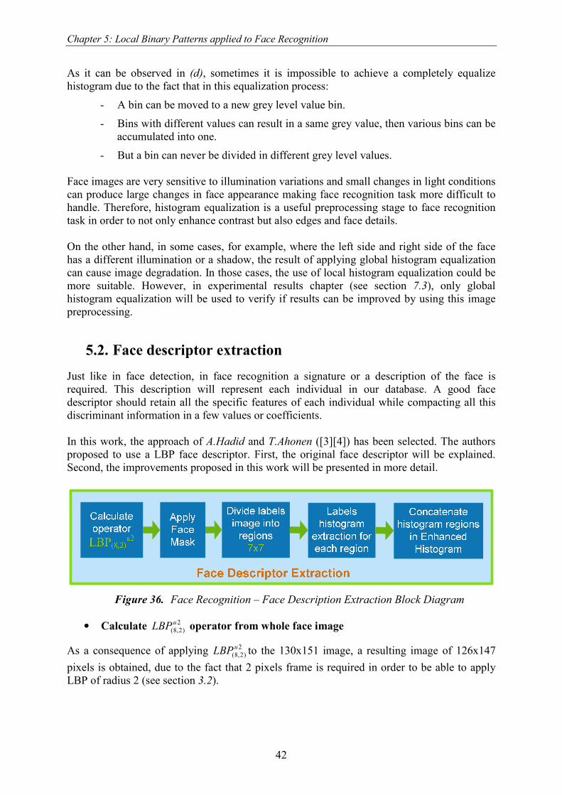
Chapter 5: Local Binary Patterns applied to Face Recognition
42
As it can be observed in (d), sometimes it is impossible to achieve a completely equalize
histogram due to the fact that in this equalization process:
- A bin can be moved to a new grey level value bin.
- Bins with different values can result in a same grey value, then various bins can be
accumulated into one.
- But a bin can never be divided in different grey level values.
Face images are very sensitive to illumination variations and small changes in light conditions
can produce large changes in face appearance making face recognition task more difficult to
handle. Therefore, histogram equalization is a useful preprocessing stage to face recognition
task in order to not only enhance contrast but also edges and face details.
On the other hand, in some cases, for example, where the left side and right side of the face
has a different illumination or a shadow, the result of applying global histogram equalization
can cause image degradation. In those cases, the use of local histogram equalization could be
more suitable. However, in experimental results chapter (see section 7.3), only global
histogram equalization will be used to verify if results can be improved by using this image
preprocessing.
5.2. Face descriptor extraction
Just like in face detection, in face recognition a signature or a description of the face is
required. This description will represent each individual in our database. A good face
descriptor should retain all the specific features of each individual while compacting all this
discriminant information in a few values or coefficients.
In this work, the approach of A.Hadid and T.Ahonen ([3][4]) has been selected. The authors
proposed to use a LBP face descriptor. First, the original face descriptor will be explained.
Second, the improvements proposed in this work will be presented in more detail.
Figure 36. Face Recognition – Face Description Extraction Block Diagram
• Calculate 2
)2,8(
uLBP operator from whole face image
As a consequence of applying 2
)2,8(
uLBP to the 130x151 image, a resulting image of 126x147
pixels is obtained, due to the fact that 2 pixels frame is required in order to be able to apply
LBP of radius 2 (see section 3.2).

Chapter 5: Local Binary Patterns applied to Face Recognition
43
• Apply face mask
The above mentioned researchers propose the application of a mask (see Figure 37) in order
to avoid non face parts in the image. As it will be explained in later experimental results
chapter 7.3, if the image is later divided in blocks and an appropriate weight value wi is
applied to each one, then the same effect can be achieved, at the same time that this extra step
can be saved. Nevertheless, in face recognition experiments this mask will be used to verify
the effect of using it.
Figure 37. Image mask example
• Divide labels image into several regions (7x7 block of 18x21 pixels)
As a good compromise between face image description and resulting feature vector length
(7x7 blocks x 59-bin/block = 2891), a 7x7 window division is proposed as a best choice for
image recognition in T.Ahonen [1].
Figure 38. LBP(8,2)u2 image example of size 126x147: 7x7 blocks of 18x21 pixels
• Labels histogram extraction for each region
Considering m facial regions R0, R1, ..., Rm-1, the LBP labels histogram is computed for each
region. In our case m is 7x7 regions.
The histogram of each block in the labeled image ),( yxf l can be defined as
{ }∑ −===yx
li niiyxfIH,
1,...,0,),( (46)
in which n is the number of different labels produced by the LBP operator and
{ }
=falseisA
trueisAAI
,0
,1 (47)
Region’s histogram provides information about the distribution of the local textures, such as
edges, spots and flat areas, over the whole image. For this reason, an efficient face
representation is achieved because spatial information is kept.

Chapter 5: Local Binary Patterns applied to Face Recognition
44
• Concatenate labels histogram of each region
Finally, each region histogram is concatenated in a spatially enhanced histogram defined as:
{ } { }∑ −=−=∈==yx
jlji mjniRyxIiyxfIH,
, 1,...,0,1,...,0,),(),( (48)
This vector will be used as a face descriptor for face recognition and in our particular case; its
length will be 2891 samples (7x7 blocks x 59-bin/block).
In experimental results chapter (see section 7.3), a combination of experiments is proposed in
order to decide the use of the different optional processings: histogram equalization, mask
and blocks weights. After them, the use of a mask is discarded, as the blocks weights are able
to perform the same functionality.
5.3. Face identification
Once the database is prepared and the spatially enhanced histograms are extracted from each
identity face, T.Ahonen and A.Hadid, in [3] and [4], proposed Chi Square algorithm as a basic
dissimilarly metric in order to compare each incoming face with the available database
identities.
As it will be later exposed in experimental results chapter, this method provides satisfactory
results, but as a contribution to this research work, it can be improved at the same time that
face descriptor dimensionality is reduced by eliminating redundant information using
Principal Component Analysis approach.
Before exposing these dissimilarly metrics, next section gives an overview of face regions
analysis to take advantage of human face recognition system to improve artificial recognition
systems.
5.3.1. Face Regions Analysis
As already exposed in face detection chapter, section 4.3.1.2, dividing the face image in
different regions can help to emphasize face features with essential information for face
description and to remove irrelevant information by using an adequate weight value.
Obviously, nose, mouth and eyes regions are likely to provide more important information in
face description task, than bottom left and right blocks where normally background areas, hair
and even cloth can be present. Moreover, neurophysiologic studies based on face recognition
human system evidence that most important face features are eyes and eyebrows, followed by
mouth and nose (see [28][29]).
Therefore, and taking into account human system knowledge, Figure 39 shows a possible
good choice for weighting face areas in face recognition procedure.

Chapter 5: Local Binary Patterns applied to Face Recognition
45
(a) Face regions weights (b) LBP(8,2)u2 image with 7x7 regions
Figure 39. Face regions weights sample taking into account human recognition system
In experimental results chapter, different sets of block weights are defined taking into account
above assumptions in order to later decide, in a empirically way, the combination to produce
best classification results.
5.3.2. Dissimilarly Metrics
5.3.2.1. Chi Square
For face identification task, first a model for each identity, Mi, is required and the simplest
way is to calculate the mean value of the N enhanced histograms of each identity. Another
possibility is to choose one image under each different illumination for each individual. Doing
this way the illumination problems can be reduced at the expense of a higher computational
cost. On the other hand, the simplest option is to select just one image as a representative
model of the individuals, although the problem will be to find out the best image of the ID
dataset that can represent the whole dataset.
Once the models are obtained, training stage is finished and a dissimilarly metrics for
histograms is required to compare input samples with the Mi models. In [4], the following
methods are proposed:
- Histogram Intersection:
∑=i
ii MSMSD ),min(),( (49)
- Log-Likelihood Statistic:
∑−=i
ii MSMSL log),( (50)
- Chi Square Statistic:
∑+
−=
i ii
ii
MS
MSMS
22 )(
),(χ (51)
Where S is the current feature vector sample, M is one identity model.
1 1 1 1 1 1 1
4 4 4 1 4 4 4
4 4 4 2 4 4 4
1 1 2 2 2 1 1
0 1 1 1 1 1 0
0 1 3 3 3 1 0
0 1 1 1 1 1 0

Chapter 5: Local Binary Patterns applied to Face Recognition
46
All these measures can be extended to the spatially enhanced histogram by summing up over
each face region. Taking Chi Square Statistic as the best option for this face recognition
application (proposed by A.Hadid and T.Ahonen), it can be extended for each region and also
a different weight can be given for each image block.
∑+
−=
ji jiji
jiji
jwMS
MSwMS
, ,,
2
,,2)(
),(χ (52)
where wj is the weight for region j.
As already exposed in section 5.3.1, in experimental results chapter will be empirically found
out the most suitable wj weight value for each j region that will enable to achieve a notable
identification ratio of 98.74%.
5.3.2.2. Principal Component Analysis
Chi Square Statistic is an adequate method to compare input 2891-bin feature vector to each
ID model and experimental results chapter will show the satisfactory (more than 98%)
identification ratios achieved. Nevertheless, by experimenting with block weights, it comes
the idea that some of the blocks seem to be more important than others, in terms of face
description, and that some feature elements may be correlated or simply not given enough
significant information to the identification task.
Therefore, it is decided to use the already implemented Principal Component Analysis, tested
in Face Detection task, to remove redundant information from enhanced face recognition
feature vector.
Application to face recognition
Following Face Detection section 4.3.2 Principal Component Analysis and focusing in face
recognition application, the method consists of computing the eigenvectors of the input 2891-
bin feature vectors taking into account all available samples of all individuals participating in
the identification scheme or at least a representative sample of length equal to input vector
length.
Enhanced feature vector in face recognition task contains 2891 elements, a quite huge number
of elements. For that reason, PCA is an interesting technique to reduce data dimensionality by
avoiding irrelevant information.
In order to decide the L significant eigenvectors, a commitment between data dimensionality
reduction and relevant information (% Info) preservation is required. Therefore, the most
suitable L number is empirically decided by maximizing the positive identification ratio of the
particular system.
Then, in the training stage not only the mean model Mi of each individual is calculated but
also the PCA matrix using input individual samples. The mean models will be stored after
projecting them to the orthonormal basis in order to reduce models number of elements from
D to L elements.

Chapter 5: Local Binary Patterns applied to Face Recognition
47
In the identification task:
� The stored Mi models are back-projected (see Figure 17).
� For each input face, the enhanced feature vector is computed.
� Then, the enhanced feature vector is projected and back-projected to the L
eigenvectors of the PCA transformation matrix to remove irrelevant information.
� Finally, the minimum distance to Mi will identify the individual face under study.
The comparison between the input sample, Si, and the model, Mi, could be also done in the
projected space but it is done in the back-projected (original space) in order to be able to use
face region weights.
As it will be demonstrated in experimental results, after adjusting the optimal number of
eigenvectors to be discarded, this method is able to improve identification ratio from 98.74%
to 99.14%.
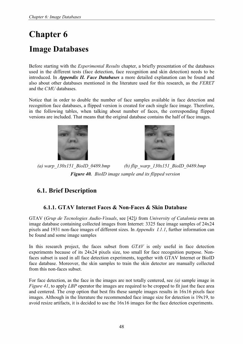
Chapter 6: Image Databases
48
Chapter 6
6.Image Databases
Before starting with the Experimental Results chapter, a briefly presentation of the databases
used in the different tests (face detection, face recognition and skin detection) needs to be
introduced. In Appendix II. Face Databases a more detailed explanation can be found and
also about other databases mentioned in the literature used for this research, as the FERET
and the CMU databases.
Notice that in order to double the number of face samples available in face detection and
recognition face databases, a flipped version is created for each single face image. Therefore,
in the following tables, when talking about number of faces, the corresponding flipped
versions are included. That means that the original database contains the half of face images.
(a) warp_130x151_BioID_0489.bmp (b) flip_warp_130x151_BioID_0489.bmp
Figure 40. BioID image sample and its flipped version
6.1. Brief Description
6.1.1. GTAV Internet Faces & Non-Faces & Skin Database
GTAV (Grup de Tecnologies Audio-Visuals, see [42]) from University of Catalonia owns an
image database containing collected images from Internet: 3325 face image samples of 24x24
pixels and 1931 non-face images of different sizes. In Appendix I.1.1, further information can
be found and some image samples
In this research project, the faces subset from GTAV is only useful in face detection
experiments because of its 24x24 pixels size, too small for face recognition purpose. Non-
faces subset is used in all face detection experiments, together with GTAV Internet or BioID
face database. Moreover, the skin samples to train the skin detector are manually collected
from this non-faces subset.
For face detection, as the face in the images are not totally centered, see (a) sample image in
Figure 41, to apply LBP operator the images are required to be cropped to fit just the face area
and centered. The crop option that best fits these sample images results in 16x16 pixels face
images. Although in the literature the recommended face image size for detection is 19x19, to
avoid resize artifacts, it is decided to use the 16x16 images for the face detection experiments.

Chapter 6: Image Databases
49
(a) nova1.bmp (24x24) (b) 16x16_nova1.bmp
Figure 41. Original image sample and its 16x16 face extraction result
Also for face detection experiments, non-faces subset is used. It contains 1931 images of
different sizes, of which around 65000 samples of 19x19 pixels size (to be compatible with
BioID 19x19 face samples) are randomly extracted to be used for face detection experiments
as non-faces samples.
For skin detector training stage, several skin images with different skin tones (different races),
illumination conditions and camera calibrations are required. They are manually collected
from GTAV Internet database, as its sample images are colored, resulting in a training set of
85 skin images with a total of 9,163 skin pixel samples.
Figure 42. Skin samples from GTAV Internet database
6.1.2. BioID Faces Database
Briefly, the BioID Face Database is used in both detection and recognition experiments and it
contains 1521 images (384x286) having only one face from 23 different persons, with a
large variety of illumination, background and face size. Moreover, each image, labeled
BioID_xxxx.pgm, has its corresponding BioID_xxxx.pts file containing 20 additional feature
points, which are very useful for facial analysis and gesture recognition.
In Appendix I.1.2, detailed information can be found about the database itself and the
procedure followed to adapt these images to our experiments.
An example of the result of this adjustment can be observed in below Figure 43, where (a) is
the original image, (b) is the adapted version for face detection and (c) for recognition
purpose.
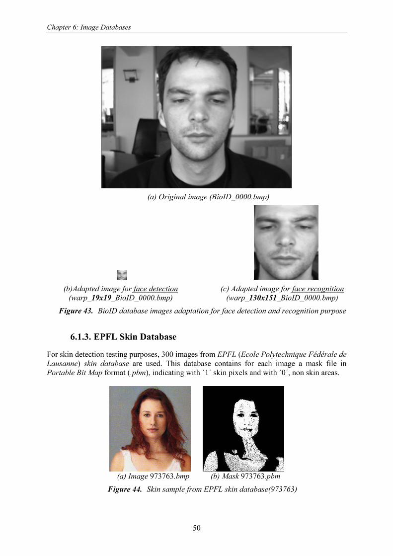
Chapter 6: Image Databases
50
(a) Original image (BioID_0000.bmp)
(b)Adapted image for face detection
(warp_19x19_BioID_0000.bmp)
(c) Adapted image for face recognition
(warp_130x151_BioID_0000.bmp)
Figure 43. BioID database images adaptation for face detection and recognition purpose
6.1.3. EPFL Skin Database
For skin detection testing purposes, 300 images from EPFL (Ecole Polytechnique Fédérale de
Lausanne) skin database are used. This database contains for each image a mask file in
Portable Bit Map format (.pbm), indicating with ´1´ skin pixels and with ´0´, non skin areas.
(a) Image 973763.bmp (b) Mask 973763.pbm
Figure 44. Skin sample from EPFL skin database(973763)

Chapter 6: Image Databases
51
6.2. Face Detection
In order to build an appearance-based detection scheme, large training sets of images are
needed in order to capture the variability of facial appearances.
Training Subset
In the training subset all the available face images have been used and as it can be observed in
next Table 7, in case of non-faces images, approximately the same number of samples has
been taken to be used together with GTAV database and about the double to be used together
with BioID database.
On the other hand, notice that the total number of negative samples will be iteratively
increased when using the bootstrap strategy (see section 4.4.1.1) in the training process.
TRAINING # Faces # Non Faces
Experiment Database
Name # Samples
Image
Size
Database
Name # Samples *
Image
Size
1 GTAV 6650 from 6650 16x16 GTAV 6605 16x16
2 Bio ID 2981 from 2981 19x19 GTAV 6605 19x19
Table 7. Training Subsets for face detection (*before bootsraping)
Test Subset
Due to the reason that it is very important to have the largest training set available, all face
samples are used in the training subset and only a portion is used for test purpose.
The non faces images number is selected so that the sum of faces and non faces is 65536:
TEST # Faces # Non Faces
Experiment Database
Name # Samples
Image
Size
Database
Name # Samples
Image
Size
1 GTAV 2000 from 6650 16x16 GTAV 63536 16x16
2 Bio ID 1500 from 2981 16x16 GTAV 64036 16x16
Table 8. Test Subsets for face detection
Parameters
The relationship between image size before and after applying LBP operator, block dimension
and overlapping is described by the following formulas:
rHEIGHTMINIMGHEIGHTMINIMG
rWIDTHMINIMGWIDTHMINIMG
GOVERLAPPINDIMBLOCKGOVERLAPPINNO
GOVERLAPPINGOVERLAPPINNOHEIGHTMINIMG
GOVERLAPPINGOVERLAPPINNOWIDTHMINIMG
2'____
2'____
__
)3_('__
)3_('__
+=
+=
−=
+×=
+×=
(53)
where r is the LBP operator radius.
And ′ indicates the image size after applying LBP operator, reduced due to the borders
treatment when applying LBP operator of radius r.

Chapter 6: Image Databases
52
6.2.1. Reference Image
In order to visually compare different face detection methods a reference image is selected to
perform this task.
Next figures shows reference image that contains 10 faces with size around the minimum size
in this research project (16x16 and 19x19) and with some areas, like the knees, with some
kind of “face appearance” that can lead to misclassification.
Figure 45. Reference image equipop.jpg (319x216 pixels)
6.3. Face Recognition
A part from the Internet face database for face detection purposes, GTAV group has another
interesting face database for face recognition testing, see [43], with 240x320 pixels images in
BMP format. This database includes a total of 44 persons with 27 images per person with
different pose views (from 0º to ±90º) and under three different illuminations. But it is
decided not to use it because no face features points files are available, requiring a pre-manual
marking of the interest point to be able to crop them to the desired size and form.
For that reason, in face recognition experiments the BioID database is selected containing:
- An amount of 23 different IDs from men and women.
- For each image the faces points file is available, then it is easy to crop faces to the
desired size.
- For each ID, there are samples with different illumination and pose.
Training and Test Subsets
All the available samples are used for both training and testing.

Chapter 6: Image Databases
53
TRAINING/TEST # Faces
# IDs Database
Name # Samples
Image
Size
23 Bio ID 3042 130x151
Table 9. Training and Test Subsets for face detection
However, for training proposes some aberrant samples has been not taken into account, like
the following affected by the image adaptation pre-process (see Appendix I.1.2).
Figure 46. BioID Database aberrant sample after image adaptation process
Therefore, in next Table 10, it can be observed that in some cases the number of samples used
for each individual for training is lower than for testing, where also the aberrant samples has
been taken into account.
Training Samples
(Mean Value
Model) Test Samples
ID1 188 216
ID2 120 120
ID3 194 194
ID4 80 80
ID5 198 198
ID6 4 4
ID7 113 118
ID8 152 156
ID9 168 176
ID10 176 176
ID11 120 122
ID12 133 142
ID13 212 212
ID14 297 298
ID15 184 188
ID16 100 100
ID17 102 102
ID18 70 70
ID19 80 80
ID20 12 12
ID21 92 92
ID22 102 102
ID23 50 50
Table 10. Training and Test Subsets for face recognition
And the following figure shows the image representation selected for each ID subset:

Chapter 6: Image Databases
54
Figure 47. BioID Database 23 different identities

Chapter 7: Experimental Results
55
Chapter 7
7.Experimental Results
In this chapter, empirical results of previous sections theory, both face detection and
recognition, are exposed. First section is dedicated to Skin Segmentation as a previous step to
face detection testing.
In order to better understand this chapter, next Figure 48 is intended to give an overview of
the experimental section flow. As it can be observed, there are three main blocks: Skin
Detection, Face Detection and Face Recognition.
Figure 48. Experimental Results Overview

Chapter 7: Experimental Results
56
Each block, can be seen as an independent system with two basic stages: training and test.
Thus, images set for each stage is required. As they will directly influence in the final
performance of the system, the appropriate selection of the images databases takes an
important role. Therefore in some cases, such as the face detection experiments, two different
databases will be used to compare results. In previous Chapter 6, image databases used for
each experiment are introduced.
In Figure 48, on the right side of each block, most important parameters of each block are
listed. In case of having such a large number of unknown variables, a coarse to fine
adjustment is recommended, where some initial values are proposed based in the system
knowledge, then the system is trained and tested with the different options and afterwards the
best option is taken and fine adjusted.
Furthermore, for simplicity in the experiments, some variables are treated independently
although they may have an influence in later stages.
7.1. Skin Detection Experiments
This section is intended to describe skin detection experimental results following 4.4.2.1 Skin
Segmentation theory chapter.
The training stage consists of manually select skin areas in collected images, in this case,
from GTAV Internet database. The main idea is to have several skin images with different
skin tones, illumination conditions and camera calibrations. Then extract chromaticity
information, u and v mean values (see equation (35)), in order to be able to define skin
decision thresholds.
Using skin training database (see section 6.1.3), the u and v mean values is computed for each
training block of size defined by equation (36). The result is shown in following Figure 49,
where the u and v mean values for each training block from 85 skin training data images
(9,163 points) are represented together with 363 non skin data images (36,300 points). In
yellow the defined skin region.

Chapter 7: Experimental Results
57
Figure 49. Skin area definition: u and v mean values plot
As explained in section 4.4.2.1 Skin Segmentation, for simplicity, a rectangle is used as a skin
region definition. The resulting border limits used as skin thresholds are the following:
=
==
=
==
140max
67minThresholds
104max
71minThresholds
v
vv
u
uu
(54)
For the test stage, equation (37) defines the skin detection box size. In this research, two
minimum face sizes are used depending on the face database: 16x16 and 19x19. For that
reason, the resulting skin detection box size for both cases is 4x4 pixels.
Once the u and v chromaticity coordinates mean value of each skin detection box is calculated,
the above thresholds are applied in order to decide if the box is labeled as skin or not.
In order to validate, the skin detection method 300 images from EPFL skin database are used
in the test stage resulting in the following results:
True Positive False Positive
pre-mask 98.68 % 72.67 %
skin mask 98.45 % 72.91 %
Table 11. Skin detection results using EPFL skin database
Above Table 11 shows the detection ratios in case of using the pre-mask and the final skin
mask of the:

Chapter 7: Experimental Results
58
- True Positives: skin pixels correctly detected as skin.
- False Positives: non-skin pixels wrongly detected as skin.
As already exposed in section 4.4.2.1, note that pre-mask is the result of applying skin model
thresholds and skin mask is the final mask resulting of applying morphological operations to
the pre-mask.
In order to be able to correctly interpret these results, it has to be taken into account that the
pre-mask post processing with morphological operations is intended to:
� Detect face skin rather than skin: therefore, skin regions smaller than the minimum
face size are removed.
� Uniform mask: without holes due to eyes and mouth areas because in face detection
process, each new block under analysis will be classified as skin if 95% of the pixels
are marked as skin. Therefore, pixels are evaluated taking into account their
neighborhood and also dilation is used to achieve uniform mask.
Moreover, any object with “skin” color is detected as skin.
In following Figure 50, all these factors can be observed. For instance, notice that:
- The difference between the pre-mask (c) and the final mask (d) is that the areas
smaller than a face resolution have been removed.
- The difference between original mask (b) and our process masks (c)(d) is that the
first one labels each single pixel individually and in (c)(d) uniform mask are
achieved.
- In pre-mask (c), it can be observed that also non skin areas with skin color are
labeled as skin. In that particular case, after morphological operations, in (d) it is
removed because the size is smaller than face resolution.
(a) Original (b) pbm_Mask (c) skinPreMask (d) skinMask (e) Result
Figure 50. Skin sample from EPFL skin database (2209950): masks comparison
Now, Table 11 results can be interpreted and understand why they are very good for this
particular face detection application:
• False positives are very high because our process is:
- detecting not only skin but also non-skin objects with skin color.
- using uniform masks. In final skin mask, false detection ratio is higher than
in pre-mask because dilation is applied.
• True positives is not 100% because our process is:
- removing skin areas smaller than face resolution, therefore the detection
ratio is lower in final skin mask than in pre-mask.
- using a different skin criterion in some difficult cases such as the one
shown in next Figure 51.

Chapter 7: Experimental Results
59
(a) Original (b) pbm_Mask
(c) skinMask (d) Result
Figure 51. Skin sample from EPFL skin database (886043): different skin criterion
The following samples are the result of performing the skin segmentation procedure using 2
moving scan pixels and 1.2 down-sampling (see section 4.1). The original reference image is
shown together with different down-sampling steps masks.
(a) Original image (b) Skin detection result (100% scale)
(c) Pre-mask (100% scale) (d) Skin mask (100% scale)

Chapter 7: Experimental Results
60
(e) Pre-mask (69.44% scale) (f) Skin mask (69.44% scale)
(g) Pre-mask (33.49% scale) (h) Skin mask (33.49% scale)
Figure 52. Skin segmentation example 1 (case 16x16): equipop.jpg
(a) Faces composite original image (100% scale)
(a) Pre-mask (23.26% scale) (b) Skin mask (23.26% scale) (c) Skin result (23.26% scale)
Figure 53. Skin segmentation example 2 (case 16x16): faces_composite_1.jpg
As seen in theory chapter 4.4.2.1, applying morphological operations improves significantly
the resulting mask by eliminating:
- Dark and small elements like the eyes and mouth in a face. This effect can be
observed in Figure 53.
- Skin regions smaller than the minimum face size. That can be clearly observed
in above Figure 52, where small skin regions like arms, legs or hands smaller
than 16x16 are removed.
Spending this time in skin segmentation will save a lot of time when exploring an image for
face detection. The time improvement is difficult to quantify, because it obviously depends on
the image type and background. The method will be very useful in case of having one person
in a field with a green background and blue sky, but not in case of having an image with
plenty of people or a color background similar to skin color like brown or orange.

Chapter 7: Experimental Results
61
7.2. Face Detection Experiments
Before implementing the face detection method proposed in the literature, Support Vector
Machine, a first approach to LBP potential is done by means of simpler classification methods.
In order to build an appearance-base detection scheme, large training sets of face images are
needed to capture the facial appearance variability. Moreover, it is no easy to find the best
non-faces set that best describe all non-faces texture possibilities. Therefore, a first random
set is collected from different images and then a bootstrap strategy of different iteration is
applied.
As explained before, this bootstrap strategy consists of training the system, classifying the
non-faces training set and reintroducing several times non-faces that are wrongly classified in
the training set until a trade-off between faces and non-faces correct detection ratios is
reached.
For each experiment the same number of test image (see Table 12) is used.
TEST images
faces 2000
non faces 63536
total 65536
Table 12. Number of test images used in every experiment
Table 13 contains the different parameters used for each face database in face detection
experiments and taking into account (53) equations:
Faces set
Parameters[pixels] GTAV
Internet BioID
Minimum Image Width 16 19 Before LBP
Minimum Image Height 16 19
Minimum Image Width 14=(4x3)+2 17=(4x3)+5
Minimum Image Height 14 17
Blocks Dimension 6=4+2 9=4+5 After LBP
Overlapping factor 2 5
Table 13. Face detection parameters for both face databases
Image size difference before and after applying LBP is due to the borders treatment when
applying LBP operator of radius 1:
• LBP(4,1) in 1st stage.
• LBP(8,1) in 2nd
stage.
7.2.1. Chi Square Classification
As it will be later seen in face recognition experiments, very satisfactory results can be
achieved by using this simple dissimilarly metric, called Chi Square (see section 4.3.1).
Because of this, it was decided to use it also for evaluating LBP face detection capability.

Chapter 7: Experimental Results
62
7.2.1.1. Non Weighted
Using non weighted Chi Square scheme, two experiments are performed with different face
databases. These tests give an idea of the quality of each face database.
For instance, GTAV Internet face database contains approximately twice the number of face
images that contains BioID face database. Consequently, it can be supposed that GTAV
Internet will describe better the face appearance variability. On the other hand, GTAV Internet
set does not have the recommended size of 19x19 (see [5]) for LBP face detection method,
but BioID has it. That means, that maybe BioID can offer better classification results.
Therefore, a part from evaluating LBP face detection potential, the aim of the following
experiments is also to find an answer to these questions.
Figure 54 presents the classification result using mean value models and Chi Square
dissimilarly metric. For each bootstrap iteration of the training process, first plot displays
faces (in orange) and non-faces (in blue) detection ratio for 16x16 GTAV Internet database
and second for 19x19 BioID database. Detailed information about the plotted values can be
found in Table 32 (16x16) and Table 33 (19x19) in Appendix III.1.2.
Figure 54. Bootstrap to improve Mean Models & Chi Square classification ratio (16x16 & 19x19)
At each bootstrap iteration, face detection rate is decreasing but non-faces detection is
increasing. This is an unavoidable compromise in order to be able to correctly classify such a
huge class as it is non-faces one.
As already exposed in section 4.4.1.1, sometimes it is not possible to converge to a point of
no false detections and a commitment between detection ratio drop and false alarm ratio
improvement is required. Therefore, the best selection should be the intersection between both
curves. For instance, taking the first bootstrap iteration for 16x16 case and the second or third
iteration for 19x19 case.

Chapter 7: Experimental Results
63
Notice that in 19x19 case, although convergence needs more iterations than in 16x16 case, the
reached point achieves better results in terms of face correct classification rate.
As a first conclusion, mean value models with Chi Square is an easy classification method
that provides satisfactory classification rates and it is useful to observe LBP qualities as a face
descriptor.
On the other hand, BioID seems to have better qualities as a face dataset. But from a realistic
point of view, GTAV Internet faces set contains a wider range of different faces than BioID
faces set which samples correspond to only 23 different people. Because of this, as the test
samples are more similar to the training ones in BioID better results can be achieved.
Therefore, let us compare both training results classifying a reference image that has nothing
to do with both face databases. In both cases, skin segmentation is used in order to improve
face detector scheme, see Figure 52. Each face candidate is marked with a yellow box and
after overlapping detections removal (see section 4.4.2.2) only one box (in red) is kept per
face.
Figure 55. Chi Square - ref img classification using GTAV Internet training set (16x16)
The result using GTAV Internet as training samples can detect the 10 faces but non faces
misclassification is very high. As faces set contains 2000 totally different faces from 2000
different people, face appearance variations is very high and a mean model of the LBP
enhanced histogram is not enough to separate faces from non faces, because regions with non
flat texture are misclassified as faces.
Figure 56 shows the results of classifying the reference image with BioID faces as training set.
Figure 56. Chi Square - ref img classification using BioID training set (19x19)

Chapter 7: Experimental Results
64
Compared to previous result, BioID training samples provides better results when classifying
non faces, although only 6 from 10 faces are correctly detected. Nevertheless, notice that
misclassified faces have a size in the limit or below of detection resolution, 19x19. Moreover,
non faces classification appears in some regions with texture similar to a face.
As a conclusion, BioID faces set and size 19x19 offer better general detection ratios. However,
this classification method, Chi-Square with mean value models, is not good enough to discern
between faces and non-faces. LBP enhanced histograms mean value models are not able to
correctly represent whole faces and non faces samples sets.
7.2.1.2. Weighted
One option to improve previous results is to use a different weight for each block of the 2nd
classification stage as proposed for face recognition.
The following table shows the result of using different weights when classifying test data. The
mean models used for each face database is the one resulting from its last bootstrap iteration.
Notice that left columns, in green, display the 3x3 block weight.
16x16 GTAV Internet 19x19 BioID
% Faces % Non Faces % Faces % Non Faces
1 1 1
(1) 1 1 1
1 1 1
78.30% 99.41% 78.55% 99.61%
1 1 1
(2) 1 2 1
1 1 1
78.45% 99.29% 77.90% 99.63%
1 1 1
(3) 1 1 1
0 1 0
78.50% 99.12% 75.55% 99.22%
1 1 1
(4) 1 2 1
0 1 0
78.45% 98.83% 74.45% 99.29%
1 2 1
(5) 1 2 1
1 1 1
78.90% 99.37% 78.15% 99.60%
1 2 1
(6) 1 2 1
0 1 0
78.70% 99.00% 74.85% 99.27%
Table 14. Weighted blocks results in 2nd classification stage for both face databases
As it can be observed in previous table, for GTAV Internet faces set using different blocks
weight a better faces classification is achieved, but non faces decreases in all cases.
On the other hand, for BioID better results are obtained by giving more weight to the central
block (2).

Chapter 7: Experimental Results
65
In next figures, it can be observed the classification improvement for the reference image for
both face databases.
For 16x16 faces case, the face detection ratio is kept while decreasing non faces
misclassification:
Figure 57. Chi Square Weighted (2) - ref img classification using GTAV training set (16x16)
On the other hand, for 19x19 faces case, faces and non-faces detection ratio increase. Notice
that now 7 from 10 faces have been correctly detected.
Figure 58. Chi Square Weighted (2) - ref image classification using BioID training set (19x19)
It can be concluded that Chi Square method is improved when using block weights in LBP
second fine stage. However, although Chi Square is an interesting approach to discover LBP
potential but it is not good enough for a valid face detection scheme.
7.2.2. Principle Component Analysis
As explained in previous chapter (see section 4.3.2), in a first approach, one PCA orthonormal
basis for both faces and non faces is calculated in order to minimize data dimensionality. And
then, in a second approach, another experiment is proposed using only faces class.

Chapter 7: Experimental Results
66
7.2.2.1. Face/Non Face Models & Relative Difference Normalized
In this chapter, the target is to find out the optimal number of eigenvalues to reduce data
dimensionality without much data loss and keeping an adequate detection ratio.
The training and test data used for these experiments are the already introduced in Table 7 and
Table 8. Following Figure 59 show the normalized eigenvalues5 plots for both databases and
for the 1st and 2
nd stage:
Figure 59. Face detection PCA - Normalized eigenvalues plot: 1st stage
The eigenvalues for both face databases are similar, although it can be observed that the
BioID two first eigenvalues have a higher value than the first two GTAV Internet eigenvalues.
That means that by keeping only two eigenvalues, a better reconstruction can be achieved
with BioID face database. Moreover, in both cases, only with this first eigenvalue more than
50% of the information is kept.
5 Normalized Eigenvalues: 1=⇒= ∑
∑ i
i
i
i
λλ
λλ
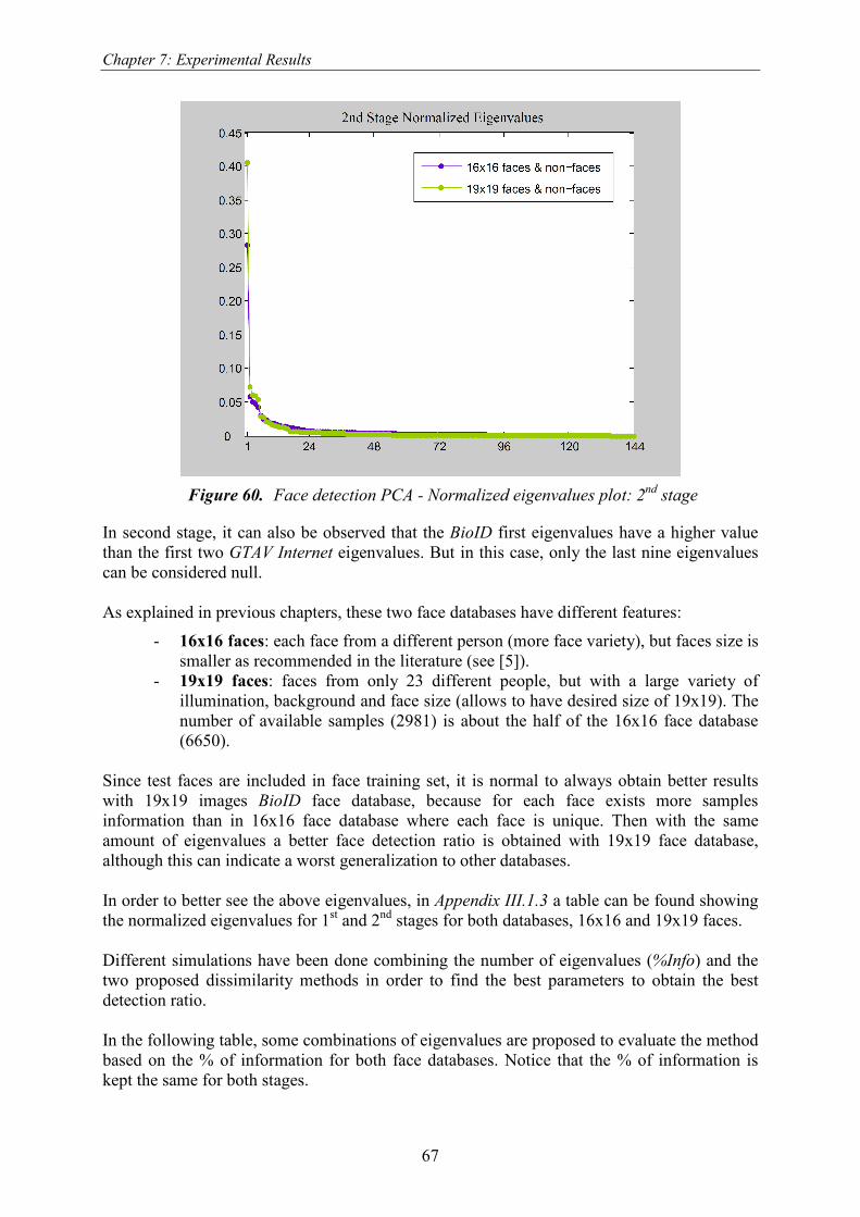
Chapter 7: Experimental Results
67
Figure 60. Face detection PCA - Normalized eigenvalues plot: 2nd stage
In second stage, it can also be observed that the BioID first eigenvalues have a higher value
than the first two GTAV Internet eigenvalues. But in this case, only the last nine eigenvalues
can be considered null.
As explained in previous chapters, these two face databases have different features:
- 16x16 faces: each face from a different person (more face variety), but faces size is
smaller as recommended in the literature (see [5]).
- 19x19 faces: faces from only 23 different people, but with a large variety of
illumination, background and face size (allows to have desired size of 19x19). The
number of available samples (2981) is about the half of the 16x16 face database
(6650).
Since test faces are included in face training set, it is normal to always obtain better results
with 19x19 images BioID face database, because for each face exists more samples
information than in 16x16 face database where each face is unique. Then with the same
amount of eigenvalues a better face detection ratio is obtained with 19x19 face database,
although this can indicate a worst generalization to other databases.
In order to better see the above eigenvalues, in Appendix III.1.3 a table can be found showing
the normalized eigenvalues for 1st and 2
nd stages for both databases, 16x16 and 19x19 faces.
Different simulations have been done combining the number of eigenvalues (%Info) and the
two proposed dissimilarity methods in order to find the best parameters to obtain the best
detection ratio.
In the following table, some combinations of eigenvalues are proposed to evaluate the method
based on the % of information for both face databases. Notice that the % of information is
kept the same for both stages.

Chapter 7: Experimental Results
68
16x16 19x19
Number of Eigenvalues Number of Eigenvalues % Info
1st Stage 2nd Stage % Info
1st Stage 2nd Stage
51% 1 6 58% 1 4
75% 4 23 79% 3 12
90% 14 56 90% 9 28
95% 25 79 95% 18 48
100% 58 135 100% 58 135
100% 59 144 100% 59 144
Table 15. Face detection PCA: number of eigenvalues selection based on %Info for
both face DB
Using above combinations of number of eigenvalues, the systems are trained and both test
data classified. Next table shows the result of these experiments:
16x16 19x19
Eigenvalues Detection
Ratio Eigenvalues
Detection
Ratio
Eigenvalues
reduction ~%
Info 1st
Stage
2nd
Stage Faces
Non
faces
~%
Info 1st
Stage
2nd
Stage Faces
Non
faces
Ratios
Sum
1st
Stage
2nd
Stage
100% 59 144 0.9940 0.6377 100% 59 144 0.9860 0.6701 3.2878 0% 0%
100% 58 135 0.9940 0.6377 100% 58 135 0.9860 0.6701 3.2878 2% 6%
95% 25 79 0.9940 0.6368 95% 18 48 0.9860 0.6693 3.2861 58% 45%
90% 14 56 0.9940 0.6353 90% 9 28 0.9855 0.6672 3.2820 76% 61%
75% 4 23 0.9935 0.6294 79% 3 12 0.9850 0.6628 3.2707 93% 84%
51% 1 6 0.9835 0.5690 58% 1 4 0.9880 0.5445 3.0850 98% 96%
Figure 61. Face detection PCA: mean detection ratio for different % of information
The column Ratios Sum is the sum of the 4 detection ratios (faces and non faces for both
databases). This value is calculated to determinate the best global detection ratio.
The row in yellow is the proposed option for the face detection system under study. A good
compromise between eigenvalues reduction and global detection ratio is the followed
criterion.
The following experiments are based in the above selection and Figure 62 presents the
classification result using PCA & Relative Difference Normalized as dissimilarly metric. For
each bootstrap iteration of the training process, first plot displays faces (in orange) and non-
faces (in blue) detection ratio for 16x16 GTAV Internet database and second for 19x19 BioID
database. Detailed information about the plotted values can be found in Table 35 (16x16) and
Table 36 (19x19) in Appendix III.1.3.

Chapter 7: Experimental Results
69
Figure 62. Bootstrap to improve PCA & RelDiffNorm classification ratio (16x16 & 19x19)
At each bootstrap iteration, face detection rate is decreasing but non-faces detection is
increasing, an unavoidable compromise in order to be able to correctly classify such a huge
class as non faces set.
As already exposed previous section, best selection should be the intersection between both
curves. For instance, taking the first bootstrap iteration for 16x16 case and the second or third
iteration for 19x19 case.
Notice that in 19x19 case, although convergence needs more iterations than in 16x16 case, the
reached point achieves better results in terms of face correct classification rate. But on the
other hand, it is also interesting to observe that when the number of bootstrap iterations
increases, faces detection ratio drops more drastically in case of 19x19 faces size. From that,
it can be deduced that 16x16 face database is capable of providing more stable results in terms
of generalization, as face detection ratio is less affected by the non-faces classes training set.
As a first conclusion, this classification method provides also satisfactory classification rates
and it is useful to observe LBP qualities as a face descriptor.
It can also be extracted that GTAV Internet faces seems to have better qualities as a face
dataset and it achieves better generalization results due to the fact that contains a wider range
of different faces than BioID faces.
As in previous chapter, the reference image (equipop.jpg, see Figure 52) is used to compare
both results. In both cases, skin detector is used in order to improve face detection scheme.
Each face candidate is marked with a yellow box and no boxes post processing is applied to
keep only one box per face. The result is given by simply applying a boxes mask.

Chapter 7: Experimental Results
70
Figure 63. PCA & RelDiffNorm - ref img classification using GTAV Internet training set
The result using GTAV Internet as training samples can detect the 10 faces but non faces
misclassification is very high. As faces set contains 2000 totally different faces from 2000
different people, face appearance variations is very high and a mean model of the LBP
enhanced histogram is not enough to separate faces from non faces, because regions with non
flat texture are misclassified as faces.
Next Figure 64 shows the results of classifying the reference image with BioID faces set as
training samples.
Figure 64. PCA & RelDiffNorm - ref img classification using BioID training set
Compared to previous result, BioID training samples provides better results when classifying
non faces, although only 3 from 10 faces are correctly detected. In this case, the price to
correctly detect non faces is too high for faces set.
As a conclusion, it is difficult to decide the best face database option and bootstrapping does
not offer the desired final converging results. The effort to reduce input vectors does not lead
into a better classification ratio. Therefore, it can be concluded that LBP enhanced histograms
mean value models together with PCA and relative difference normalized are not able to
correctly represent whole faces and non faces samples sets.

Chapter 7: Experimental Results
71
7.2.2.2. Only Faces & Threshold
As explained in previous chapters, one of the most important problems is the complexity of
representing non faces class:
- Non faces samples can go from total flat textures to extremely granulated ones.
Because of this, it is really difficult to represent such a wide class with a unique
enough representative model.
- Some textures can have a similar LBP feature vector to faces one, that means that
faces samples are included in non faces LBP space.
Then, it can be reasonable that only taking into account faces model and an appropriate
threshold faces can be correctly classified.
Each input vector is projected in the orthonormal matrix for faces class, and then back-
projected. Finally the resulting reconstructed vector is compared to the original one. If the
distance is less than a give threshold then it will be classified as a face.
See previous section 4.3.2.2 for more detailed information.
Using only the face training samples for both databases the eigenvalues and thresholds are
extracted.
Training Faces
Database Name # Samples Image Size
GTAV Internet 6650 16x16
Bio ID 2981 19x19
Table 16. PCA only faces: Number of samples for each face detection training set.
The following figures show the normalized eigenvalues plots for both databases and for the 1st
and 2nd
stage:
Figure 65. Face detection PCA only faces - Normalized eigenvalues plot: 1st stage

Chapter 7: Experimental Results
72
Figure 66. Face detection PCA only faces - Normalized eigenvalues plot: 2nd stage
The eigenvalues for both face databases are similar, only in the first stage it can be observed
that the BioID first eigenvalues has a higher value than the first GTAV Internet eigenvalues.
That means that by keeping only one eigenvalue, a better reconstruction can be achieved with
BioID face database.
For both databases, in first stage the last eigenvalue and in second stage the last nine
eigenvalues are zero.
The behavior of these eigenvalues is similar to the case of having both negative and positive
samples, as seen in previous chapter.
The next step consists of deciding:
- An appropriate number of eigenvalues to keep for each stage. The idea is to have
enough eigenvalues to have an acceptable loss rate between original and
reconstructed image.
- K1stStg and 2ndStgK values to adjust the decision threshold for each stage. Once or
twice the deviation should be a proper threshold, but in order to observe the
evolution for different K, values between 1 and 6 are evaluated. For simplicity,
integer values have been used, although for fine adjustment decimals could be used.
In order to better see the above eigenvalues, in Appendix III.1.3 a table can be found showing
the normalized eigenvalues for 1st and 2
nd stages for both databases, 16x16 and 19x19 faces.
Comparing this table with the one from previous chapter, see Appendix III.1.3, it can be
observed that in the other case the information was more concentrated in first eigenvalues.
Just the first eigenvalue has the double information when taking into account faces and non-
faces dataset. That can be due to the fact that number of samples is much higher when taking
also into account non-faces samples.

Chapter 7: Experimental Results
73
Another interesting point is that in this case, the relation between % information and number
of eigenvalues between both face databases is more similar just taking into account faces
samples. In the following table some combination of eigenvalues are proposed to evaluate the
method:
16x16 19x19
Number of Eigenvalues Number of Eigenvalues % Info
1st Stage 2nd Stage % Info
1st Stage 2nd Stage
25% 1 3 29% 1 3
46% 3 10 45% 3 7
54% 5 15 54% 5 12
70% 13 31 70% 13 23
90% 34 72 90% 36 57
100% 59 144 100% 59 144
Table 17. PCA only faces: number of eigenvalues selection based on % of Info
Different simulations have been performed combining the number of eigenvalues (%Info) and
K values in order to compare both databases and investigate the possibilities of this method.
And finally select the best parameters to obtain the best detection ratio.
Table 18. PCA only faces: detection ratio for different K1st and K2nd, eigenvalues

Chapter 7: Experimental Results
74
At first sight, it is not obvious the best parameters combination, but it is noticeable that:
- The lower the K values the best compromise between faces and non faces detection
ration.
- As seen in previous experiments, face detection ratio must be penalized in order to
achieve a better non faces detection ratio.
- In first stage, better non faces detection ratio is achieved with 19x19 face database.
- An inflection point exists for the number of eigenvalues to be selected in both
cases. Taking into account more eigenvalues does not represent any detection ratio
improvement.
In order to decide the best % of information (number of eigenvalues) to obtain the best
detection ratio for all cases (faces and non faces, and for both face databases) the mean
detection ratio is calculated:
- In each cell: faces and non faces mean detection ratio.
- In horizontal: mean detection ratio for different K1st and K2nd values.
- In vertical: mean detection ratio for different number of eigenvalues.
Figure 67. PCA only faces: mean detection ratio for different # eigenvalues and K values
Then it can be concluded that the best choice for both databases to achieve the optimum
detection ratio for both faces and non faces is:
- K1stStg=1 and K2ndStg=2
- About 45-46% information, that means:
� 3 eigenvalues for the 1st stage
� 7-10 eigenvalues for the 2nd
stage.
Next step is to classify both test databases with the selected parameters. As the detection
ratios are slightly different for near K1stStg and K2ndStg values, two more combinations are used
to check the resulting detection ratio.

Chapter 7: Experimental Results
75
Figure 68. Mean detection ratio of faces and non faces for 45-46% of information and different K values.
In this case the best option is to select K1stStg=2 and K2ndStg=1. Moreover, using K1stStg > K2ndStg
allows to be less restrictive in 1st coarse stage and more restrictive in the final 2
nd fine stage.
Finally, in order to compare results with the other exposed methods, let us compare training
results classifying the reference image that has nothing to do with both face databases. In both
cases, skin detector is used in order to improve face detection scheme.
Each face candidate is marked with a yellow box and no boxes post processing is applied to
keep only one box per face. The result is given by simply applying a boxes mask.
Figure 69. PCA Only Faces - ref image classification using GTAV Internet training set (16x16)
Figure 70. PCA Only Faces - ref image classification using BioID training set (19x19)
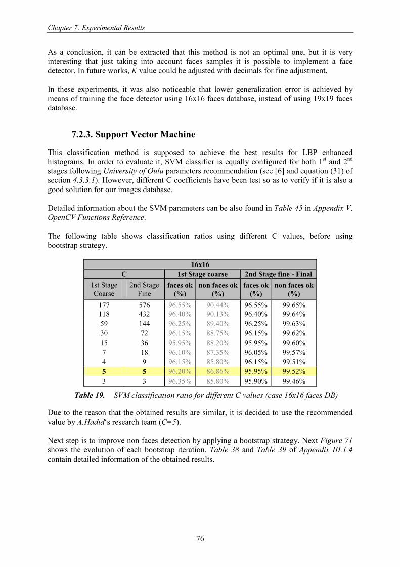
Chapter 7: Experimental Results
76
As a conclusion, it can be extracted that this method is not an optimal one, but it is very
interesting that just taking into account faces samples it is possible to implement a face
detector. In future works, K value could be adjusted with decimals for fine adjustment.
In these experiments, it was also noticeable that lower generalization error is achieved by
means of training the face detector using 16x16 faces database, instead of using 19x19 faces
database.
7.2.3. Support Vector Machine
This classification method is supposed to achieve the best results for LBP enhanced
histograms. In order to evaluate it, SVM classifier is equally configured for both 1st and 2
nd
stages following University of Oulu parameters recommendation (see [6] and equation (31) of
section 4.3.3.1). However, different C coefficients have been test so as to verify if it is also a
good solution for our images database.
Detailed information about the SVM parameters can be also found in Table 45 in Appendix V.
OpenCV Functions Reference.
The following table shows classification ratios using different C values, before using
bootstrap strategy.
16x16
C 1st Stage coarse 2nd Stage fine - Final
1st Stage
Coarse
2nd Stage
Fine faces ok
(%)
non faces ok
(%)
faces ok
(%)
non faces ok
(%)
177 576 96.55% 90.44% 96.55% 99.65%
118 432 96.40% 90.13% 96.40% 99.64%
59 144 96.25% 89.40% 96.25% 99.63%
30 72 96.15% 88.75% 96.15% 99.62%
15 36 95.95% 88.20% 95.95% 99.60%
7 18 96.10% 87.35% 96.05% 99.57%
4 9 96.15% 85.80% 96.15% 99.51%
5 5 96.20% 86.86% 95.95% 99.52%
3 3 96.35% 85.80% 95.90% 99.46%
Table 19. SVM classification ratio for different C values (case 16x16 faces DB)
Due to the reason that the obtained results are similar, it is decided to use the recommended
value by A.Hadid‘s research team (C=5).
Next step is to improve non faces detection by applying a bootstrap strategy. Next Figure 71
shows the evolution of each bootstrap iteration. Table 38 and Table 39 of Appendix III.1.4
contain detailed information of the obtained results.

Chapter 7: Experimental Results
77
Figure 71. Bootstrap to improve SVM classification ratio (16x16 & 19x19 faces)
From above graphs, it can be extracted that best classification results are achieved before
applying bootstrap strategy, because faces detection ratio is highly penalized when trying to
improve non faces detection ratio. But on the other hand, compared to previous experiments,
in that case it is possible to nearly reach 100% of correct detections in non faces case. As
already mentioned, non faces dataset contains a wide range of possible textures that make
difficult the use of a mean model as a reference to compare with new input samples. Therefore,
SVM method is capable of defining a better threshold regions between both faces and non-
faces classes, achieving a better classifier.
Using reference image to compare this method with previous ones, following Figure 72
shows the result of applying SVM with C=5.
Figure 72. SVM - reference image classification using GTAV training set (16x16)
For that case, all faces are still correctly detected and only 3 non faces are misclassified: two
knees and one throat.

Chapter 7: Experimental Results
78
Then, the same procedure is applied to 19x19 face database in order to compare the
robustness of the method in front of the faces database. Following Figure 73 shows the result
of classifying the reference image:
Figure 73. SVM - reference image classification using BioID training set (19x19)
For 19x19 case, all faces non faces are correctly classified but only 3 faces are correctly
classified from 10. As already exposed, BioID face database contains less faces samples than
GTAV Internet face database and moreover, the faces are for only 23 different people.
Because of this, very good results are achieved when classifying training and test data, but not
when classifying the reference image. Because of this, it can be concluded that GTAV Internet
provides a lower generalization error.
7.2.3.1. Additional 3rd stage: SVM score thresholds
In this research work, as a contribution to the two stages face detection scheme introduced by
University of Oulu researchers, a third stage is proposed to improve final detection results by
setting empirical thresholds to avoid non faces misclassification.
For next experiments, only GTAV Internet database (16x16 face images) will be used, as it
has been generally providing best face detection results.
In order to decide 3rd
stage thresholds, some GTAV Internet faces samples are classified for
the purpose of collecting SVM scores for the 1st and 2
nd stages. Next Table 20 shows statistical
information of the obtained scores.
Scores 1stStg 2ndStg 1stStg+2ndStg
Average -0.6053 -3.8947 -4.5000
StdDev 0.4375 1.2742 1.4669
Min -2.5243 -9.4057 -11.2732
Max -0.0007 -0.7344 -1.5225
Table 20. SVM scores from 3281 faces
Resulting from above table, the following values are settled as thresholds in a third stage to
decide the final faceness of the image:

Chapter 7: Experimental Results
79
Threshold 1stStg + 2ndStg = -1.5
Threshold2ndStg = -0.5
The flowchart to be followed is shown in next figure:
2nd Stage COARSE
1st Stage FINE
16x16
image
block
Result_1stStg = 1?
Result_1stStg = 1?
3rdStage FINAL
(Score1stStg+Score2ndStg)
<Threshold1stStg+2ndStg&
Score2ndStg<Threshold2ndStg
?
NON
FACE
NO
NO
NO
YES
YES
YES
FACE
NON
FACE
NON
FACE
Figure 74. SVM faces classification flowchart with addition 3rd stage
The reason why this 3rd
stage improves face classification results is because it is capable of
avoiding non-faces misclassifications which results in an aberrant score far from the mean
value one.
The improvement achieved with this method can be observed in the following sample images,
in yellow intermediate face detections and in red final decision after overlapping boxes
removal:

Chapter 7: Experimental Results
80
Figure 75. SVM with 3rd Stage classification (16x16): equipop.jpg
Comparing Figure 72 with above Figure 75, it can be observed how this extra stage is
capable of removing false face detections: two knees, with round form and face like
appearance, while keeping face detection ratio.
Not only good results are achieved for the reference image, but also for the following sample
images:
Figure 76. SVM with 3rd Stage classification (16x16): boda.jpg
In above Figure 76, no false detections appear, but one face is misclassified due to the fact
that the system in not trained on purpose to detect rotated faces. Notice that at least the other
rotated face is correctly detected. Therefore, the system could still improved by introducing
rotated samples to the face training set.

Chapter 7: Experimental Results
81
Figure 77. SVM with 3rd Stage classification (16x16): faces_composite_1.jpg
In above Figure 77, all faces are correctly detected but in some cases as in 1st column, 2
nd row
and 3rd
row faces, the overlapping boxes removal method is not selecting the best box. In
those cases, it could be better to use Overlapping Detection Merge (see section 4.4.2.2).
Figure 78. SVM with 3rd Stage classification (16x16): CMU test-original1.bmp

Chapter 7: Experimental Results
82
In above Figure 78, the eight faces are correctly detected although there are two
misclassifications that could be avoided using the skin detector in case of having a colored
image. However, notice that the misclassified non-faces have face appearance.
Figure 79. SVM with 3rd Stage classification (16x16): CMU test- hendrix2.bmp
In above Figure 79 case, the overlapping boxes removal method is selecting the best box and
no misclassifications are detected.
7.2.3.2. PCA before applying SVM
This section is intended to improve SVM classification potential by applying a PCA pre
processing to the input samples in order to reduce data dimensionality and eliminate
redundant information.
Only GTAV Internet 16x16 face database is used in the experiment because it has already
been demonstrated that provides the best generalization results.
Taking advantage from previous section 7.2.2, dedicated to PCA. The experiments are
focused to the following number of eigenvalues (extracted from Table 15):
16x16
Number of Eigenvalues % Info
1st Stage 2nd Stage
90% 14 56
95% 25 79
Table 21. Face detection PCA (16x16 case): best number of eigenvalues selection
Next figures show the bootstrap strategy evolution, where it can be observed that face
detection ratio drops drastically compared to previous approaches. See Table 40 and Table 41
in Appendix III.1.5 for detailed information.
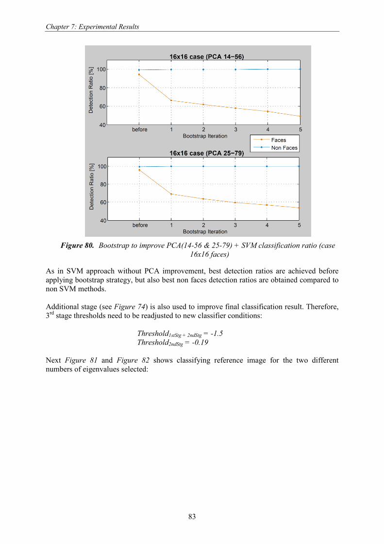
Chapter 7: Experimental Results
83
Figure 80. Bootstrap to improve PCA(14-56 & 25-79) + SVM classification ratio (case 16x16 faces)
As in SVM approach without PCA improvement, best detection ratios are achieved before
applying bootstrap strategy, but also best non faces detection ratios are obtained compared to
non SVM methods.
Additional stage (see Figure 74) is also used to improve final classification result. Therefore,
3rd
stage thresholds need to be readjusted to new classifier conditions:
Threshold1stStg + 2ndStg = -1.5
Threshold2ndStg = -0.19
Next Figure 81 and Figure 82 shows classifying reference image for the two different
numbers of eigenvalues selected:

Chapter 7: Experimental Results
84
Figure 81. PCA(14_56)+SVM faces classification: equipop.jpg
Figure 82. PCA(25_79)+SVM faces classification: equipop.jpg (Moving step = 1)
As a conclusion of these last experiments, a reduction of the input data dimensionality
provides also satisfactory results although a clearly improvement is not achieved.
7.3. Face Recognition Experiments
This section describes face recognition experimental results following chapter 5 proposed
approaches.
As already explained, face recognition method based in LBP approach consists of extracting a
2891 features vector consisting of ( (7x7 blocks) x 59-bin/block) for each input face sample of
a given individual in order to create a mean features vector model for each person in the
database. Once a new person is to be identified, the LBP features vector is calculated and
compared to the stored ID models.
First of all, the original work ([1][3][4]) of simply using Chi Square as dissimilarly metric in
the identification task will be under study and then it will be improved by means of Principal
Component extraction in order to remove redundant information and enhance identification
ratio.

Chapter 7: Experimental Results
85
The BioID database will be used for face recognition experiments and the number of samples
used in training and test stages is shown in Table 10. Training and Test Subsets for face
7.3.1. Chi Square Dissimilarly Metric
In face recognition experiments using Chi Square as dissimilarly metric, some pre and post
processing methods will be used in order to verify its impact on identification ratio, such as:
- Use of a mask: to avoid non face parts in the face image with no useful
information for the identification task (see Figure 83).
- Histogram equalization: in order to perform a contrast adjustment to normalize
face images to be compared.
- Blocks weight: to emphasize face elements containing relevant information in face
recognition task such as the eyes or mouth. After testing different features weights,
Figure 84 shows the two block weight best options.
- Model type: use of only 1 representative image of the individual for the features
vector model or mean value of individual’s face samples for the model.
Figure 83. Face mask used in face recognition testing
The combination of above approaches leads to 10 different experiments that, for simplicity,
will be named from Test1 to Test10.
The results will be presented in three steps, each one fixing the kind of block weights used
and combining the use of histogram equalization and mask.
Histogram equalization versus Mask
using no Block Weight
Histogram equalization versus Mask
using Block Weight (1)
Histogram equalization versus Mask
using Block Weight (2)
Test
1
Test
2
Test
3
Test
4
Test
5
Test
6
Test
7
Test
8
Test
9
Test
10
Equalized
Histogram x x � � x � � x � �
Mask x � x � x x � x x �
Blocks
Weight x x x x �(1) �(1) �(1) �(2) �(2) �(2)
Table 22. Face recognition experiments overview
And to be concluded, a results table (Table 26) will help to overview the obtained results and
to select the best options.
� Histogram equalization versus Mask using no Block Weight
Next table shows first experiments combining the use of a mask and histogram equalization
for the case of mean value model and 1 image model (see section 5.3.2.1). The last row

Chapter 7: Experimental Results
86
presents the mean ID recognition ratio in %, calculated by weighting each ID ratio by its
number of samples, due to the fact that the number of samples for each ID is different (see
Table 10) and each sample requires the same importance. The complete table with the
individual results can be consulted in Appendix IV.1.1.
Test 1 Test 2 Test 3 Test 4
Equalized Histogram x x � �
Mask x � x �
Blocks Weight x x x x
Type Model 1 Img Mean 1 Img Mean 1 Img Mean 1 Img Mean
57.48% 97.87% 55.75% 97.27% 57.95% 97.74% 55.78% 97.31% ID Recognition Rate
77.67% 76.51% 77.84% 76.54%
Table 23. ID recognition rate (%). Histogram equalization versus Mask
The use of mean value model considerably increases the face recognition ratio compared to
the case of using 1 image as mean model. Nevertheless, it can be noticed that in some cases 1
image is enough to correctly identify the other faces in the database, in case of low face
variations in group set.
Comparing above values, best results are achieved for mean value model case when using
neither histogram equalization nor mask, and for 1 image model case when using only
histogram equalization. However, taking into account both case models results, the highest
score is achieved in case of using only histogram equalization.
� Histogram equalization versus Mask using Block Weight (1)
Next step consists of using block weights to highlight face relevant information such as the
eyes and the mouth and avoid irrelevant or very variable information.
In order to find out best weighting blocks, each individual block of the 7x7 blocks should be
used alone in the recognition task to find out its significance and to decide its weight. For
simplicity and taking into account theory section 5.3.1 Face Regions Analysis, University of
Oulu experience (see [1]) and after some preliminary testing the following weighting map are
selected as best candidates:
Figure 84. Features weight comparison and its corresponding recognition rate
Observing above feature masks, most importance is given to eye area and mouth, removing
areas with irrelevant information such as the background on bottom sides. Another interesting
point to notice is that best results are achieved by removing nose septum area, the least
important face feature (see section 5.3.1).
2 1 1 1 1 1 2 1 1 1 1 1 1 1
2 4 4 1 4 4 2 1 4 4 1 4 4 1
1 1 1 0 1 1 1 1 1 1 0 1 1 1
0 1 1 0 1 1 0 0 1 1 0 1 1 0
0 1 1 1 1 1 0 0 1 1 1 1 1 0
0 1 1 2 1 1 0 0 0 1 2 1 0 0
0 1 1 1 1 1 0 0 0 1 1 1 0 0
features weight (1) features weight (2)
98.44% 97.27%

Chapter 7: Experimental Results
87
The following tables combine the use of above features weight (1) with the use of mask and
histogram equalization.
Test 5 Test 6 Test 7
Equalized Histogram x � �
Mask x x �
Blocks Weight �(1) �(1) �(1)
Type Model 1 Img Mean 1 Img Mean 1 Img Mean
62.76% 98.60% 63.00% 98.74% 62.20% 98.44% ID Recognition Rate
80.68% 80.87% 80.32%
Table 24. ID recognition rate (%). Histogram equalization versus Mask using Block
Weight (1)
In this case, the best option also considers the use of histogram equalization as a pre
processing step of face samples. Additionally, the identification ratio is increased by using the
Block Weight (1).
� Histogram equalization versus Mask using Block Weight (2)
The same procedure is followed with Block Weight (2).
Test 8 Test 9 Test 10
Equalized Histogram x � �
Mask x x �
Blocks Weight �(2) �(2) �(2)
Type Model 1 Img Mean 1 Img Mean 1 Img Mean
61.60% 97.34% 62.00% 97.27% 62.00% 97.27% ID Recognition Rate
79.47% 79.63% 79.63%
Table 25. ID recognition rate (%). Histogram equalization versus Mask using Block
Weight (2)
In this case, the best results are achieved by using histogram equalization and using a mask so
as not the same results are obtained.
Summary
Next table and plots are intended to collect all above results to better visualize the best results.
It shows the ID recognition rate (%) for each different test and for both model type, using
only 1 representative image of each individual.
Test
1
Test
2
Test
3
Test
4
Test
5
Test
6
Test
7
Test
8
Test
9
Test
10
Equalized
Histogram x x � � x � � x � �
Mask x � x � x x � x x �
Blocks
Weight x x x x �(1) �(1) �(1) �(2) �(2) �(2)
Mean Model 97.87% 97.27% 97.74% 97.31% 98.60% 98.74% 98.44% 97.34% 97.27% 97.27%
1 Img Model 57.48% 55.75% 57.95% 55.78% 62.76% 63.00% 62.20% 61.60% 62.00% 62.00%
77.68% 76.51% 77.84% 76.55% 80.68% 80.87% 80.32% 79.47% 79.64% 79.64%
Table 26. ID recognition rate (%) for each experiment and for both model types

Chapter 7: Experimental Results
88
Summarizing, the best results are obtained for Test 6 with a 98.74% of correct identification
ratio:
- No mask.
- Histogram equalization.
- Blocks weight (1).
- Mean model type.
As already exposed, no mask is needed if blocks weight is used because the same target is
achieved by given a low value to the bottom side of the image, where normally image
background, cloths or hair are to be found.
Moreover histogram equalization (see section 5.1) is improving face recognition task by
counteracting light conditions that affect face appearance by enhancing contrast and at the
same time, edges and face details.
Obviously mean model type is the best option, because it is difficult to find out the best image
of the ID dataset that can represent the whole dataset. Although from this research
experiments in 1 image model case, it can be extracted that our representative ID face
selection can describe around 60% of its ID set.
Concluding, it has been demonstrated that by using LBP enhanced histogram and a simply
dissimilarly metric very satisfactory results are achieved.
7.3.2. Principal Component Analysis
Following section is intended to improve above results using Principal Component Analysis
in order to remove redundant information and enhance identification ratio. Experiments will
focus on Test 6 (no mask, histogram equalization, block weight (1) and mean model type) but
also in Test 3 (no mask, histogram equalization, no block weight and mean model type) due to
the fact that PCA itself will weight the most important blocks in the face image. Therefore,
theory suggests that best results can be achieved with Test 3 case.
Following the already explained procedure (see section 5.3.2.2), the covariance matrix C is
computed in order to calculate eigenvectors matrix V, together with its corresponding
eigenvalues. Different strategies can be followed, but in this case, it is decided to have a
unique V matrix calculated using all available data, 2947 face samples, for following reasons:
� A representative transformation matrix for each ID is discarded because: the
number of available samples for each ID is different (see Table 10), in some cases
only 4 samples are available and it is undesirable to manage 23 different
eigenvectors matrixes.
� In our concrete case, the number of available samples, 2947, is in the range of the
number of elements in the enhanced features vector. Then, the eigenvectors length
will be the minimum value between the number of input samples and the input
samples length, namely 2891 eigenvectors.
( )lengtht samples ples, inpu#input samors#eigenvect min= (55)

Chapter 7: Experimental Results
89
Following table shows the number of eigenvectors selected for the experiments based in
eigenvalues information. First column is the number of eigenvectors selected, second column
is the last eigenvalue, third column is the last normalized eigenvalue, fourth column is the
accumulative information of the number of eigenvectors selected, fifth column is the
percentage of eigenvectors selected and the last column is the eigenvectors reduction achieved.
# Eigenvalue Norm Eigenvalue % Accumulative Info % Eigenvectors
1 0.10162122 0.08160000 8.16% 0.03%
62 0.00304733 0.00244690 75.20% 2.14%
88 0.00183365 0.00147240 80.09% 3.04%
233 0.00043843 0.00035200 90.01% 8.06%
484 0.00014275 0.00011460 95.00% 16.74%
723 0.00007679 0.00006170 97.00% 25.01%
1446 0.00001906 0.00001530 99.37% 50.02%
2024 0.00000535 0.00000430 99.88% 70.01%
2830 0.00000001 0.00000000 100.00% 97.89%
2842 0.00000000 0.00000000 100.00% 98.31%
2891 0.00000000 0.00000000 100.00% 100.00%
Table 27. PCA for face recognition: eigenvalues information
Analyzing the obtained eigenvalues, keeping only 25% (~750) of the eigenvectors, about
97.5% of the original vectors information still remains. Moreover, just by keeping 2842 of
2891 eigenvectors (1.69% reduction), no information is lost due to the fact that last 49
eigenvalues have nearly zero value.
While implementing PCA approach applied to face recognition, it was noticed that due to
reconstruction error, in some cases, negative or aberrant values appeared when back-
projecting feature vectors samples. As a consequence, corrections on Chi Square formulation
are submitted to avoid the effect of these undesired values and in order to improve
identification ratios. Therefore, in the experimental results, these 3 cases are used:
� Norm (Model + Feature):
∑+
−=
ji jiji
jiji
jwMS
MSwMS
, ,,
2
,,2)(
),(χ (56)
� Norm (Model):
∑−
=ji ji
jiji
jM
MSw
, ,
2
,,
modelNorm
2
w
)(χ (57)
� No Norm:
∑ −=ji
jijij MSw,
2
,,noNorm
2
w )(χ (58)
After above considerations, following figure shows the results of experimenting with Test3
and Test6, for mean models, keeping different number of eigenvectors and with three Chi
Square formulations:

Chapter 7: Experimental Results
90
Figure 85. Face Identification Ratios for different number of eigenvalues
Here, the effect of the reconstruction error can be clearly observed when the input feature
sample S is kept in the denominator of the Chi Square formulation. In case of obtaining
aberrant or negative values after back projecting, keeping S in the denominator can provide
undesired and unrealistic low results if S is very high or high results if S is very low.
Therefore, most interesting results are obtained when keeping only the model M in the
denominator that a priori is not providing aberrant values in the reconstruction process.
Focusing in the case of using Chi Square only normalized by the model value, next figure is a
zoom of above figures. In this representation, it is important to note that it is possible to
improve face identification system up to 99.14% by keeping only around 723 eigenvectors in
Test 3 case. Therefore, the use of block weight can already be left aside.

Chapter 7: Experimental Results
91
Figure 86. Norm (Model) Face Identification Ratios
Before, taking 723 as the value that maximizes the identification ratio, an exploration of the
nearby values is performed to find out if another maximum exists.
Next table shows already used values, in gray, and the new ones under investigation, in black.
# Eigenvalue Norm Eigenvalue % Accumulative Info % Eigenvectors
1 0.10162122 0.08160000 8.16% 0.03%
62 0.00304733 0.00244690 75.20% 2.14%
88 0.00183365 0.00147240 80.09% 3.04%
233 0.00043843 0.00035200 90.01% 8.06%
484 0.00014275 0.00011460 95.00% 16.74%
585 0.00010640 0.00008540 96.00% 20.24%
649 0.00009127 0.00007330 96.51% 22.45%
703 0.00008022 0.00006440 96.88% 24.32%
704 0.00007994 0.00006420 96.89% 24.35%
705 0.00007970 0.00006400 96.89% 24.39%
708 0.00007909 0.00006350 96.91% 24.49%
713 0.00007836 0.00006290 96.94% 24.66%
718 0.00007757 0.00006230 96.97% 24.84%
723 0.00007679 0.00006170 97.00% 25.01%
728 0.00007610 0.00006110 97.04% 25.18%
733 0.00007521 0.00006040 97.07% 25.35%
921 0.00005099 0.00004090 98.00% 31.86%
1446 0.00001906 0.00001530 99.37% 50.02%
2024 0.00000535 0.00000430 99.88% 70.01%
2830 0.00000001 0.00000000 100.00% 97.89%
2842 0.00000000 0.00000000 100.00% 98.31%
2891 0.00000000 0.00000000 100.00% 100.00%
Table 28. PCA for face recognition: eigenvalues information in the nearby of
eigenvalue 723

Chapter 7: Experimental Results
92
Using above number of eigenvectors, the identification ratios are recalculated and next figure
shows the results for Test3 case.
Figure 87. Test3 – MeanModel - Norm (Model): Face Identification Ratios
As it can be observed, a maximum identification rate exists between the 703 and 733 number
of eigenvectors. Therefore, 713 is taken as the mean value of this area and selected as the best
option for face identification task with a 99.14% of identification ratio.
Summing up, the best combination of factors is to use:
� Pre processing: histogram equalization, no mask and no blocks weight.
� Mean model.
� PCA with 713 eigenvectors.
� Chi Square statistic only normalized by the model value.
Concluding it is worth to computationally invest in PCA projecting and back projecting
process, because the main target of this procedure is to avoid irrelevant information and
therefore enhancing face recognition results.
In this research, the Chi Square comparison is not performed in the projected space to be able
to apply blocks weight and follow the same procedure as the case without PCA. But after
observing that the use of mask or blocks weight is not necessary, as the PCA itself is able of
detecting and weighting the most important bins of the enhanced feature vector, for future
work it could also be interesting to make the comparison in the PCA projected space.

Chapter 8: Development Tools
93
Chapter 8
8.Development Tools
This chapter gives an overview of this research used tools, its motivation and a brief reference
manual of the implemented application FaceProcessingTool.
8.1. Programming Environment
Microsoft Visual Studio 2005 platform, together with Microsoft Visual C++ 2005
environment, is the preferred option as it provides a powerful and flexible development
environment for Windows-based application. Moreover, it enables the possibility of taking
advantage of OpenCV Library.
OpenCV Library 1.0, Intel® Open Source Computer Vision Library is a collection of C
functions and a few C++ classes that implement many popular Image Processing and
Computer Vision algorithms.
Besides, MATLAB 7.0 is also used as a numerical computing environment useful in this
research for matrix manipulation and data plotting.
8.2. Face Processing Tool
An application with a user-friendly graphical user interface (GUI) is developed implementing
face detection and recognition algorithms with the aim of helping in the training and testing
stages.
Figure 88. Face Processing Tool application main dialog
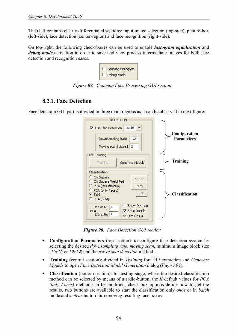
Chapter 8: Development Tools
94
The GUI contains clearly differentiated sections: input image selection (top-side), picture-box
(left-side), face detection (center-region) and face recognition (right-side).
On top-right, the following check-boxes can be used to enable histogram equalization and
debug mode activation in order to save and view process intermediate images for both face
detection and recognition cases.
Figure 89. Common Face Processing GUI section
8.2.1. Face Detection
Face detection GUI part is divided in three main regions as it can be observed in next figure:
Figure 90. Face Detection GUI section
• Configuration Parameters (top section): to configure face detection system by
selecting the desired downsampling rate, moving scan, minimum image block size
(16x16 or 19x19) and the use of skin detection method.
• Training (central section): divided in Training for LBP extraction and Generate
Models to open Face Detection Model Generation dialog (Figure 94).
• Classification (bottom section): for testing stage, where the desired classification
method can be selected by means of a radio-button, the K default values for PCA
(only Faces) method can be modified, check-box options define how to get the
results, two buttons are available to start the classification only once or in batch
mode and a clear button for removing resulting face boxes.
Configuration
Parameters
Training
Classification

Chapter 8: Development Tools
95
8.2.1.1. Skin Segmentation Training
Moreover, as a part of the face detection section, on the top-right corner of the main dialog
(see Figure 88) a Train Skin Detector button can be found for skin segmentation training.
Figure 91. Skin Detection Training Button
By clicking the above button, the following dialog appears to choose the skin samples path
and to perform the calculation of the Luv values (see section 4.4.2.1).
Figure 92. Skin Detection Training dialog
As a result, a skin_uv.txt file is obtained containing the uv mean and standard deviation values
for each processed block of size (imgWidth/10)x(imgHeight /10) of each image available.
These results are then used to define the thresholds for skin segmentation procedure.
8.2.1.2. Training
Face detection training phase is split in two stages: LBP extraction (Training Button) and
faces and non-faces models generation (Generate Models Button). The purpose of this
division is to have a first stage common to the different classification methods that extracts
the enhanced feature vector of each training sample and saves it in a training file
(LBP_ForFaceDetection_Training_NxN.txt) that will be later used to generate the models for the
different detection algorithms.
Figure 93. Face Detection LBP training GUI section
Once the LBP vectors are obtained, clicking the Training button, for face (positive) samples
and non-faces (negative) samples, the Generate Models button will open the following dialog:

Chapter 8: Development Tools
96
Figure 94. Face Detection Model Generation dialog
In order to generate the training models using above dialog:
• The paths for the positive and negative sample files have to be indicated.
• Then, the desired method can be changed by means of the Method radio-buttons.
• If the number of input positive and negative samples is different, the # Samples
radio-buttons enables to get all of them or to select a number of negative samples
(normally bigger) equal to the number of positive samples.
• The combo-box enables to switch from 16x16 to 19x19 pixels face images, for
experiments using both available databases (GTAV Internet and BioID).
• In case of selecting PCA methods, PCA Eigenvalues section allows to change the
number of desired eigenvectors for 1st coarse and for 2
nd fine stages.
The final training files will be saved in C:\LBP\ folder:
Face detection method Result files
Mean value models_NxN.txt
PCA (RelDiffNorm)
PCA_models_NxN.txt
PCA_eigenvalues_NxN.txt
PCA_eigenvectors_NxN.txt
PCA (only faces)
PCA_OnlyFaces_eigenvalues_ NxN.txt
PCA_OnlyFaces_eigenvectors_NxN.txt
PCA_OnlyFaces_MeanStdDev_NxN.txt
SVM model_SVM_1stStageCoarse_NxN.xml
model_SVM_2ndStageFine_NxN.xml
PCA (SVM)
PCA_SVM_eigenvalues_NxN.txt
PCA_SVM_eigenvectors_NxN.txt
PCA_SVM_models_1stStageCoarse_NxN.xml
PCA_SVM_models_2ndStageFine_NxN.xml
Table 29. Face Detection training stage result files

Chapter 8: Development Tools
97
8.2.1.3. Test
Once the training files are obtained, the test section is ready for use. But first of all, the
desired configuration parameters have to be selected in the following section to determinate
the input image exploration method:
Figure 95. Face Detection configuration parameters
• Skin segmentation preprocessing.
• Minimum image block size selection: 16x16 or 19x19.
• Downsampling rate setting.
• Moving scan selection.
Then, the face detection method under study can be chosen in the following section, together
with the type of classification (Once or Batch) and the way of showing the results:
- Show Overlap: displays intermediate face boxes before face overlapping removal.
- Live Result: displays face detection boxes result in the picture box during the
classification process. If it is unchecked, then the results are shown at the end of
the process in an image window pop-up.
- Save Result: saves results in LBP_ForFaceDetection_Class_MethodName_NxN.txt output file.
Figure 96. Face Detection classification options
Face boxes display options are not available in batch mode, where the results are just stored in
an output file.
On the lower-left corner, the K default values for PCA (only Faces) method for 1st and 2
nd
stages can be modified if required.
Finally, the Clear button removes resulting face boxes after face detection process.
Moreover, the face detection can be performed on:

Chapter 8: Development Tools
98
� Static images: which firstly have to be loaded and then displayed in the picture
box. The result face boxes can be also shown in the picture box if the Live Result
check-box is checked.
� Live video: that can be activated by means of Figure 97 check-box. Then, a Live
Video window is popped up showing the live captured video (see Figure 98 (a)).
For live face detection, press Once button in detection area (see Figure 96) and
two more extra windows will be displayed (see Figure 98 (b) and (c)). Live Video
window (a) will show captured video with live face detections marked with green
boxes and the two smaller windows will show the intermediate overlapped results,
(b), and the skin segmented image if the option is selected, (c), respectively.
Figure 97. Live Video mode check-box
(a) Face detection result (b) Overlapping (c) Skin Mask
Figure 98. Face detection live video result image windows
8.2.2. Face Recognition
Face recognition GUI part is also divided in three main regions as observed in next figure:

Chapter 8: Development Tools
99
Figure 99. Face Recognition GUI section
• LBP testing (top section): for LBP firstly evaluation purposes, this section allows
to extract Local Binary Patterns and calculate the labels histogram by pressing
LBP button after selecting the following configuration parameters:
- ROI combo-box: input image blocks division (7x7, 5x5, 3x3 and 1x1).
- LBP combo-box: sampling point and radius ((8,2)u2, (8,1)u2 and (4,1)).
- Show Histogram check-box: to plot in an extra window the resulting
histogram.
• Training (central section): divided in Training for LBP extraction and Generate
Models to open Face Recognition Model Generation dialog (Figure 101).
• Classification (bottom section): for testing stage, containing radio-buttons for
recognition method selection, check-boxes to select the use of a mask, the results
storage and to enable live face recognition, two buttons to start the recognition
process only Once or in Batch mode and a Clear button for removing the identified
ID face from picture box.
8.2.2.1. Training
Face recognition training phase is also split in two stages: LBP extraction (Training Button)
and ID models generation (Generate Models Button). The purpose of this division is to have a
first stage common to the different classification methods that extracts the enhanced feature
vector of each training sample and saves it in a training file
(LBP_ForFaceRecognition_Training.txt) that will be later used to generate the models for the
different recognition algorithms.
Figure 100. Face Recognition LBP training GUI section
LBP testing
Training
Classification

Chapter 8: Development Tools
100
Once the LBP vectors are obtained, clicking the Training button, for each individual, the
Generate Models button will open the following dialog:
Figure 101. Face Recognition Model Generation dialog (Mean Value)
By default, Mean Value method is selected and, as it can be observed in above image, to
obtain the mean model for each individual, the ID training file has to be selected, then the
corresponding ID # has to be indicated and, by clicking the Generate button, an ID mean
model file (see Table 30) will be outputted. This procedure has to be repeated for all available
IDs.
In case of selecting PCA method, just by clicking the Generate button the output files will be
generated taking into account all individual samples. The required number of eigenvectors to
consider can be changed in the range from 1 to 2891 enhanced feature vector elements (7x7
blocks x 59-bin).
Figure 102. Face Recognition Model Generation dialog (PCA)
The final training files will be saved in C:\LBP\IDs\ folder:

Chapter 8: Development Tools
101
Face recognition method Result files
Mean value IDX_model.txt
PCA
IDs_models_PCA_projected.txt
IDs_models_PCA_eigenvectors.txt
IDs_models_PCA_eigenvalues.txt
Table 30. Face Recognition training stage result files
8.2.2.2. Test
Once the training files are obtained, the test section is ready for use. But first of all, the
desired configuration parameters have to be selected to determinate the required input image
preprocessing and if the results have to be stored:
� Histogram equalization (see common parameters in Figure 89)
� Mask use (see Figure 103)
� Save Result (see Figure 103) to indicate that identification results have to be
stored in LBP_ForFacRecognition_Class_MethodName.txt output file.
Figure 103. ID picture-box containing identified face
Then, the face recognition method under study can be chosen in the following section,
together with the type of classification (Once or Batch) and a Clear button to remove the
identified ID face from picture box (see above Figure 103).
Moreover, the face recognition can also be performed on:
� Static images: which firstly have to be loaded and then displayed in the ID
picture-box. The result ID image is shown in Figure 103 picture-box.
� Live video: that can be activated by means of Figure 97 check-box. Then, a Live
Video window is popped up showing the live captured video (see Figure 104). For
live face recognition, check Set Frame option (see Figure 103) to display a purple
rectangle in the Live Video window to place user’s face, then when the face is set
as shown in Figure 104 sample, press Once button in recognition area (see Figure
103) and face recognition ID image result will be shown in ID picture-box.
Moreover, an extra window will show the preprocessed image: grayscale
converted and resized to face recognition 130x151 size (see Figure 104).

Chapter 8: Development Tools
102
Figure 104. Face recognition live video result image windows

Chapter 9: Conclusions
103
Chapter 9
9.Conclusions
This chapter is intended to give an overview of the complete proposal, the improvements
achieved, problems found during the research and moreover to outline future lines of work.
The extensive face analysis area implies a lot of possible or potential applications for
researchers. Applications today in the field of surveillance, banking and multimedia
equipment are becoming more and more important. For this reason, the face analysis research
community has sufficient work in order to completely solve the face detection and recognition
challenges, most important of which were discussed in section 2.3.
It is important to note that each application related to face analysis has different requirements
in the analysis process. This is the main reason why almost all algorithms and approaches for
face analysis are application dependent and a standardization or generalization is very
difficult, at least for the moment.
The panacea for all researchers involved with the face analysis research area is to be able to
emulate the human system, which is a heuristic and complicated approach taking into account
multiple clues such as textures, color, motion and even audio information. Therefore, and due
to the rapid evolution of technology that makes it possible, the recent trend is moving towards
multimodal analysis combining multiple approaches to converge towards more accurate and
satisfactory results.
Contributions to actual face detection and recognition applications are helpful to enable the
face analysis research community to continue building more robust systems by linking
different approaches and combining them. Therefore, the aim of this research is to contribute
by exploring the Local Binary Patterns operator, motivated by the following reasons. On one
hand, it can be applied to face detection and recognition, thus its implementation enables the
possibility to investigate both research fields, enabling the possibility of building a complete
system with both detection and recognition stages, all with a low computation complexity. On
the other hand, as presented in the studies [1]-[7] to demonstrate its robustness to pose and
illumination changes.
Following the working structure of this research and before reaching the experimental results
chapter, image databases selection is a vital component to take into account in order to
succeed with such a kind of learning algorithms where input samples are required to train the
system. Chapter 6 introduces the images databases used: faces, non faces and skin. Instead of
creating an own database adapted to the requirements of this research, existing databases are
used and adapted to the system necessities to save time. In the case of face detection
experiments, two different databases have been used to find out which one of them is the best
option and moreover to demonstrate how important the training samples for the final system
performance are.
The experimental results are first focused in a skin detection algorithm (see section 4.4.2.1)
used as a pre-processing stage to later speed up the face detection task, computationally
affected by its scanning algorithm used to explore images (see section 4.1 and Appendix

Chapter 9: Conclusions
104
III.1.1). The skin segmentation system implemented (see section 7.1) not only uses color
information but also tries to take into account a system’s face resolution by eliminating skin
areas smaller than the minimum possible face. The improvement achieved with this method,
in terms of efficiency, depends on the type of the input image and the background. The
method will be very useful for instances involving one unique person with a green or blue
background, but not in cases involving images of a crowded place and with a background of a
similar color to skin like brown or orange.
The next step in the experimental section concerns the face detection system, where before
implementing the face detection method proposed in the literature (see [5][6]), Support Vector
Machine, a first approach to explore LBP potential is completed by means of more simple
classification methods: Chi Square and PCA (see section 7.2.1 and 7.2.2 respectively).
Obviously the detection ratios results obtained are worse when compared to SVM results but
are sufficient enough to perceive how a simple texture operator can be used as a face
descriptor.
It should be noted that when testing PCA in face detection task (see section 7.2.2.2), non-
negligible values are obtained when using only faces samples for training the system. For
future works, it would be interesting to continue exploring the use of only face class since it is
not easy to find the best non-faces set that best describes all non-face texture possibilities.
After this first approach to LBP applied to face detection, SVM implementation (see section
7.2.3) shows the robustness of the system providing very satisfactory results as reveled in the
literature [5][6]. This research tries to go one step further and adds one extra stage to the
original two-stage system to improve face detection ratio (see section 7.2.3.1). And in
addition, it tries to eliminate redundant information from feature vectors using the PCA
method after features extraction (see section 7.2.3.2). Thereby concluding that a reduction of
the input data dimensionality also provides satisfactory results, although a clear improvement
is not achieved.
Moreover, also for future improvements, in order to increase face detection and recognition
ratios, rotated face samples should also be added to the training databases.
The last section of the experimental results is dedicated to the face recognition method (see
section 7.3). The first part consists in implementing the literature proposal [1][2][4] using Chi
Square as a dissimilarly metric in the identification task providing even more encouraging
results than in the face detection part. Different experiments are performed to improve the
identification ratio by applying different pre-processing methods such as histogram
equalization, the use of a face mask and even blocks weights (see Table 22).
In the face recognition case, the idea of using PCA to eliminate redundant information takes
more importance, since LBP enhanced featured vector for the face recognition task consists of
an excessive number of elements, 2891 to be exact (see section 5.2). Therefore, the PCA
method is applied and a more exhaustive search for the optimal number of eigenvectors is
performed, resulting in a noticeable improvement of the final identification ratios (see section
7.3.2).
In future lines of work, the face recognition systems implemented could be improved by
solving the problem of having an external individual, not present in training samples that tries
to identify itself. In the way in which it is done now, the individual will be identified with the

Chapter 9: Conclusions
105
individual ID with minimum distance, but it should be rejected by the system. Therefore,
some kind of maximum distance threshold should be used to avoid this problem.
As already reveled in Chapter 8, all the above experiments have been tested using Microsoft
Visual C++ due to the possibility of using OpenCV libraries which contain complete and
open source image processing and machine learning algorithms. Moreover, another
motivation is the possibility of creating a Windows dialog based application with a friendly
GUI to test the whole system with static images and video mode. The main intention of the
developed FaceProcessingTool application is to evaluate experiment results and it could be
improved, for example, by speeding face detection algorithm using multi threading, e.g. each
down-sampled image processed in a new thread.
For future work, the LBP method is now available in Matlab (see [44]) so it is possible to take
advantage of powerful image processing toolboxes to evaluate other method combinations.

Appendix
106
Appendix
I. Face Databases
I.1.1. GTAV Internet Face Database
One of the databases of the Grup de Tecnologies Audio-Visuals of the UPC (see [42]) used in
this research consists of:
# Faces # Non Faces
Number of samples Image Size Number of samples Image Size
3325 24x24 1931 Different sizes
Table 31. Test Subsets for face detection
Images are collected from Internet:
���� Faces set: faces are extracted from Internet images by manually marking the eye
position of each face in the image and then, by automatically collecting each face by
means of its eyes position. The resulting 24x24 faces set is a good representation of
variability of facial appearance.
Figure 105. Face image samples from GTAV Internet Face Database (100% scale)
���� Non faces set: non faces images are randomly collected from Internet. They have
different sizes, resolutions, compression factor and scenarios. Therefore, they form a
fine representation of the wide non faces class.

Appendix
107
Figure 106. Non faces image samples from GTAV Internet Face Database (scaled to different sizes)

Appendix
108
I.1.2. The BioID Face Database
http://www.humanscan.de/support/downloads/facedb.php
The BioID Face Database is public database from HumanScan, a biometric software
development company focused on multimodal biometric authentication technology.
This faces database has been recorded and published to give all researchers working in the
area of face detection the possibility to compare the quality of their face detection algorithms.
Special emphasis has been given to achieve real world conditions. Therefore the test set
contains a large variety of illumination, background and face size.
Figure 107. BioID database image samples (25% scale)
a) Description of the BioID Face Database
• 1521 gray level images.
• Resolution of 384x286 pixels.
• Each image shows one frontal view of a face.
• 23 different test persons.
• The images are labeled BioID_xxxx.pgm.
• The files BioID_xxxx.eye contain the eye positions for the corresponding images.
• The files BioID_xxxx.pts contain 20 additional feature points, which are very
useful for facial analysis and gesture recognition.

Appendix
109
b) Image File Format
The images are stored in single files using the Portable Gray Map (PGM) data format. A
PGM file contains a data header followed by the image data. In this case the header consists
of four lines of text:
• 1st line: image data format (ASCII/binary). In this case binary (indicated with P5).
• 2nd line: image width in text form (384).
• 3rd line: image height in text form (286).
• 4th line: maximum allowed gray value (255).
The header is followed by a data block containing the image data. The data is stored line per
line from top to bottom using one byte per pixel.
c) Eye Position File Format
The eye position files are text files containing a single comment line followed by the x and
y coordinate of the left eye and the x and y coordinate of the right eye separated by spaces.
Note that left eye refers to the person's left eye. Therefore, when captured by a camera, the
position of the left eye is on the image's right and vice versa.
Figure 108. Eye position file format
d) FGnet Markup Scheme of the BioID Face Database
The BioID Face Database is being used within the FGnet project of the European Working
Group on face and gesture recognition. PhD students from the department of Imaging Science
and Biomedical Engineering at the University of Manchester marked up the images from the
BioID Face Database. They selected several additional feature points, which are very useful
for facial analysis and gesture recognition.
There are 20 manually placed points with the following markup scheme:
0 = right eye pupil
1 = left eye pupil
2 = right mouth corner
3 = left mouth corner
4 = outer end of right eye brow
5 = inner end of right eye brow
6 = inner end of left eye brow
7 = outer end of left eye brow
8 = right temple
9 = outer corner of right eye
10 = inner corner of right eye
11 = inner corner of left eye
12 = outer corner of left eye
13 = left temple
14 = tip of nose
15 = right nostril
16 = left nostril
17 = centre point on outer edge of upper lip
18 = centre point on outer edge of lower lip
19 = tip of chin
#LX LY RX RY
231 99 159 98

Appendix
110
Figure 109. Image sample with its corresponding points file
In order to adequate these images to our experiments a preprocessing step is applied:
PGM to BMP conversion
Due to the fact that our application, FaceProcessingTool, only accepts JPG and BMP images,
the possibility to implement a Portable Gray Map (PGM) image reader was evaluated, but for
simplicity, it was decided to batch convert all the images to bmp.
Image crop
19x19 and 130x151 pixels face images are needed for the face detection and face recognition
application, respectively. Therefore, a subroutine was developed in order to crop all images
by means of the following points extracted from BioID_xxxx.pts file:
- Right temple (markup #8)
- Left temple (markup #13)
- Kin (markup #19)
Figure 110. The 3 points used in order to crop images and an example file (BioID_0000.pts)
version: 1
n_points: 20
{
159.128 108.541
230.854 109.176
164.841 179.633
223.237 178.998
132.469 93.9421
183.883 94.5768
211.177 95.2116
254.974 91.4031
129.295 109.176
144.529 109.811
176.901 107.272
216.89 107.272
246.088 110.445
261.957 109.811
196.578 139.009
184.518 147.261
207.369 145.991
195.943 175.189
193.404 193.597
192.769 229.143
}

Appendix
111
The image is affine warped by means of matrix affine transform using 3 points. The function
cvGetAffineTransform from OpenCV libraries calculates the matrix of an affine transform as
follows:
2..0
),(][
)','(][
:
)1,,(_)','(
=
=
=
•=
i
yxisrc
yxidst
where
yxmatrixmapyx
ii
ii
T
ii
T
ii
(59)
where:
� src is the coordinates vector of the 3 triangle vertices in the source image.
� dst is the coordinates vector of the 3 corresponding triangle vertices in the destination
image.
� map_matrix is the pointer to the destination 2×3 matrix.
The function cvWarpAffine from OpenCV transforms source image using the specified matrix:
byxmatrixmapyx
yxsrcyxdst
TT +•=
←
)1,,(_)','(
),()','( (60)
Once the image has been warped the face region is cropped.
Face Detection
In case of face detection database, the following 3 points are used in order to warp face image:
( ) 75)2(].0[].2[.].2[
2].1[].2[.].2[
].0[].1[.].1[
2].1[.].1[
.].0[.].0[
0].0[..].0[
⋅++=⇒+=
=⇒=
=⇒=
+=⇒+=
=⇒=
=⇒−=
HeightrydstydstrycvPtKinysrc
xdstxdstxcvPtKinxsrc
ydstydstyemplecvPtRightTysrc
WidthrxdstrxemplecvPtRightTxsrc
ymplecvPtLeftTeydstymplecvPtLeftTeysrc
xdstrxmplecvPtLeftTexsrc
(61)
where:
� [0] point is face left temple.
� [1] point is face right temple.
� [2] point is face kin.
� Width is face image width, after LBP(8,1): 17 pixels.
� Height is face image height, after LBP(8,1): 17 pixels.
� r is LBP radius: 1 pixels.
Then, the face region is extracted from the image:

Appendix
112
( )
)2('
)2('
72)2(].0[
].0[
0
0
rHeightHeight
rWidthWidth
Heightrydsty
xdstx
+=
+=
⋅+−=
=
(62)
(a) Original image (BioID_0000.bmp) (b) Warped and cropped result image
(warp_19x19_BioID_0000.bmp)
Figure 111. Face Detection: Image warping and cropping example
Face Recognition
In case of face recognition database, the following 3 points are used in order to warp face
image:
BlockHnYBlocksrydstydstrycvPtKinysrc
xdstxdstxcvPtKinxsrc
ydstydstyemplecvPtRightTysrc
nXBlocksBlockWrxdstrxemplecvPtRightTxsrc
ymplecvPtLeftTeydstymplecvPtLeftTeysrc
xdstrxmplecvPtLeftTexsrc
⋅−++=⇒+=
=⇒=
=⇒=
⋅+=⇒+=
=⇒=
=⇒−=
)2(].0[].2[.].2[
2].1[].2[.].2[
].0[].1[.].1[
)(2].1[.].1[
.].0[.].0[
0].0[..].0[
(63)
where:
� [0] point is face left temple.
� [1] point is face right temple.
� [2] point is face kin.
� BlockW is block width: 18 pixels.
� BlockH is block height: 21 pixels.
� nXBlocks is the number of x blocks: 7 blocks.
� nYBlocks is the number of y blocks: 7 blocks.
� r is LBP radius: 2 pixels.

Appendix
113
Then, the face region is extracted from the image:
)2(
)2(
)2(].0[
].0[
0
0
rnYBlocksBlockHHeight
rnXBlocksBlockWWidth
rBlockHydsty
xdstx
+⋅=
+⋅=
+⋅−=
=
(64)
(a) Original image (BioID_0000.bmp)
(b) Warped and cropped result image
(warp_130x151_BioID_0000.bmp) Figure 112. Face Recognition: Image warping and cropping example

Appendix
114
I.1.3. The Facial Recognition Technology (FERET) Database
http://www.itl.nist.gov/iad/humanid/feret/feret_master.html
The FERET program (1993-1997) was sponsored by the Department of Defense's
Counterdrug Technology Development Program through the Defense Advanced Research
Products Agency (DARPA). Its primary mission was to develop automatic face recognition
capabilities that could be employed to assist security, intelligence and law enforcement
personnel in the performance of their duties.
The FERET image corpus was assembled to support government monitored testing and
evaluation of face recognition algorithms using standardized tests and procedures. The final
dataset consists of 14051 eight-bit grayscale images of human heads, 1199 different persons,
with views ranging from frontal to left and right profiles.
The images contain variations in lighting, facial expressions, pose angle, etc.
I.1.4. CMU Database
This image dataset is used by the CMU Face Detection Project and is provided for evaluating
algorithms for detecting frontal views of human faces. This particular test set was originally
assembled as part of work in Neural Network Based Face Detection. It combines images
collected at CMU and MIT.
Ground truth in face location is provided in the following format with one line per face
(extreme side views are ignored):
filename left-eye right-eye nose left-corner-mouth center-mouth right-corner-mouth
For each feature on a face to be detected, two numbers are given. These numbers are the x and
y coordinates (measured from the upper left corner) of the feature in the image.
The images are in Compuserve GIF format and are grayscale. The images are available
individually or collectively in a tar file. This file will unpack into four directories:
test: containing the images in Test Set A.
test-low: containing Test Set B.
newtest: containing Test Set C.
rotated: containing the Rotated Test Set.
Test Set B was provided by Kah-Kay Sung and Tomaso Poggio at the AI/CBCL Lab at MIT,
and Test Sets A,C and the rotatated test set were collected at CMU (by Henry A. Rowley,
Shumeet Baluja, and Takeo Kanade).

Appendix
115
a) From test (to 30 reduced) b) From test-low (100)
c) From newtest (to 50 reduced) d) From rotated (to 30 reduced)
Figure 113. CMU database image samples

Appendix
116
II. Skin Chromaticity
A color can be described as a mixture of three other colors or tristimuli. The amount of each
stimulus defines the color. However, it is frequently useful to separate the color definition into
luminance (luminous intensity) and chromaticity (color information).
Each color representation system has its benefits and disadvantages depending on the
application. In case of skin representation, the most widely used are the chromaticity based
ones due to its robustness against intensity and illumination.
The evolution of the chrominance based systems is exposed in the following lines:
CIE Standard XYZ (1931)
The standard defines the positive tristimuli for all visible light sources, which can be
calculated as follows:
=
B
G
R
Z
Y
X
990.0010.0000.0
011.0813.0177.0
200.0310.0490.0
(65)
XYZ are virtual primaries, based on human eye response and metamerism effect (two light
sources can have the same apparent color to an observer).
As a result, the spectrum locus is represented as shown in the following figure (2D projection:
X+Y+Z=1):
Figure 114. Spectrum Locus
The XYZ normalized values can be also calculated as follows:
yxZYX
Zz
ZYX
Yy
ZYX
Xx −−=
++=
++=
++= 1,, (66)

Appendix
117
Mac Adam’s Ellipses
In the spectrum locus, elliptical areas with equal color can be represented, as seen next figure.
Figure 115. Mac Adam’s Ellipses
The minimum change in XYZ to appreciate chrominance variations is called JND (Just
Noticeable Difference).
As it can be observed in the figure, human eye is very sensible to variations in skin color but
not in green levels.
CIE UCS: Uniform Chromaticity Scale (1960)
Lately a uniform chromaticity representation is proposed where these ellipses become circles:
3122
6
315
6
3122
4
315
4
++−=
++=
++−=
++=
yx
y
ZYX
Yv
yx
x
ZYX
Xu
(67)
CIE LUV: Perceptual Uniformity (1976)
Some years later, a modification in the v component generates the LUV perceptual uniformity
representation:
3122
9
315
9
2
3'
315
4'
++−=
++==
++==
yx
y
ZYX
Yvv
ZYX
Xuu
(68)

Appendix
118
III. Face Detection Result
This section contains some detailed information that can help to understand face detection
experimental results.
III.1.1. Face Detection Computational Cost Analysis
In such a kind of algorithms, such as face detection, one of the most important limitations is
the algorithm speed affected by the scanning method used for input image exploration for face
candidates searching (see section 4.1).
Although two stages algorithm is proposed in order to improve efficiency, when searching in
high resolution images, using down-sampling and a moving scan smaller than one block
width the detection algorithm can be very slow.
It can be demonstrated that the total number of blocks to be analyzed can be calculated as
follows:
( ) ( )∑
−
=
−
×
−
=1#
0
#iterations
n
nn
MS
MS-tBlockHeighDS
ImgHeight
MS
MS-BlockWidthDS
ImgWidth
blocks (69)
The number of iterations in the down-sampling process can be calculated by means of the
following expressions:
∑∞
=
⋅
=
0
#n
nn DS
ImgHeighth
DS
ImgWidthwiterations (70)
where functions w(x) and h(y) are defined as follows:
<
≥=
BlockWidthxif
BlockWidthxifxw
0
1)( (71)
<
≥=
tBlockHeighyif
tBlockHeighyifyh
0
1)( (72)
and:
• DS is the down-sampling rate.
• MS is the moving scan pixels.
• ImgWidth and ImgHeight are the image size.
• BlockWidth and BlockHeight are the block size.
• n is the current iteration.
For example, in the following situation:
- VGA resolution (640x480)
- Down-sampling rate of 1.2
- Moving scan of 2 pixels
- Block size of 19x19 pixels
The number of iterations is calculated as follows:

Appendix
119
iterations .
h.
h.
witerationsn
nn
nn18
21
480
21
480
21
640#
00
=
=
⋅
= ∑∑
∞
=
∞
=
(73)
<
≥=
90
191)(
1yif
yifyh (74)
Then, the total number of blocks is:
( ) ( )
blocks
blocksn
nn
n
nn
535,223
4
711.2
48017
1.2
640
2
2-191.2
480
2
2-191.2
640
#17
0
17
0
=
=
−×
−
=
−
×
−
= ∑∑==
(75)
III.1.2. Chi Square Classification
Following section presents the classification result using mean value models and Chi Square
dissimilarly metric for the cases of weighted and non weighted blocks and for both databases:
GTAV Internet (16x16) and BioID (19x19).
Non Weighted
GTAV Internet (16x16)
The following table presents the classification result using mean value models and Chi Square
dissimilarly metric. Each row contains a bootstrap iteration with the following information
(from left to right):
• Current bootstrap iteration.
• Number of repetition of the false classified samples reintroduced in the training set.
• The number of non faces training samples incorrectly classified.
• Number of positive and negative training samples.
• Percentage of faces and non faces correctly classified.
GTAV Internet database 16x16 - mean value & chi square non weighted
Bootstrap Training Samples Correct classification
# False classified
samples repetition # False Positive Positive Negative Faces (%) Non faces (%)
Before - 1467 6650 6605 98.70% 75.45% 1 5 213 6650 13940 88.90% 94.81%
2 5 153 6650 15005 87.15% 96.46% 3 5 119 6650 15770 86.00% 97.15%
4 10 82 6650 16960 84.75% 97.89% 5 10 58 6650 17780 83.80% 98.25%
6 10 52 6650 18360 83.15% 98.47% 7 10 49 6650 18880 82.65% 98.67%
8 10 37 6650 19370 82.35% 98.79%
9 15 35 6650 19925 81.85% 98.93% 10 15 31 6650 20450 81.25% 99.00%
Table 32. Bootstrap strategy to improve Mean Models & Chi Square classification ratio
(16x16 faces)

Appendix
120
BioID (19x19)
The following figure presents the results from BioID database with 19x19face size.
BioID database 19x19 - mean value & chi square non weighted
Bootstrap Training Samples Correct classification
# False classified
samples repetition # False Positive Positive Negative Faces (%) Non faces (%)
Before - 1437 2981 6605 99.65% 71.47% 1 5 386 2981 13790 94.65% 89.81%
2 5 276 2981 15720 93.70% 92.15% 3 5 224 2981 17100 92.40% 93.50%
4 10 165 2981 19340 91.00% 95.28% 5 10 127 2981 20990 89.95% 96.35%
6 10 113 2981 22260 88.80% 97.09%
7 10 88 2981 23390 87.75% 97.65% 8 10 69 2981 24270 87.05% 98.07%
9 15 58 2981 25305 86.05% 98.42% 10 15 48 2981 26175 85.55% 98.65%
Table 33. Bootstrap strategy to improve Mean Models & Chi Square classification ratio
(19x19 faces)
III.1.3. Principal Component Analysis
Faces and Non-Faces
In order to better see the eigenvalues information, the following table shows the normalized
eigenvalues for 1st and 2
nd stages and for both databases, 16x16 and 19x19 faces. The %Info
column is the accumulated % information if eigenvalues from number 1 to n row are kept.
Norm_eigenvals_1stStageCoarse norm_eigenvals_2ndStageFine
16x16 19x19 16x16 19x19
Eigenvalue %
Info Eigenvalue
%
Info Eigenvalue
%
Info Eigenvalue
%
Info 1 0.51587569 51.59% 0.57079131 57.08% 1 0.28315487 28.32% 0.40479755 40.48%
2 0.15332067 66.92% 0.17053065 74.13% 2 0.05828740 34.14% 0.07213775 47.69%
3 0.05217609 72.14% 0.04577915 78.71% 3 0.05038590 39.18% 0.06041664 53.74%
4 0.03602537 75.74% 0.03461586 82.17% 4 0.04706113 43.89% 0.05917424 59.65%
5 0.03045715 78.79% 0.02339686 84.51% 5 0.04149003 48.04% 0.05408509 65.06%
6 0.02096952 80.88% 0.01985427 86.50% 6 0.02994824 51.03% 0.02890813 67.95%
7 0.01921549 82.80% 0.01298886 87.80% 7 0.02422030 53.45% 0.02664519 70.62%
8 0.01429545 84.23% 0.01110365 88.91% 8 0.02272362 55.73% 0.02107954 72.72%
9 0.01366349 85.60% 0.00999613 89.91% 9 0.02002354 57.73% 0.01876637 74.60%
10 0.01189272 86.79% 0.00909007 90.81% 10 0.01863823 59.59% 0.01724930 76.33%
11 0.01110972 87.90% 0.00846822 91.66% 11 0.01764229 61.36% 0.01518112 77.84%
12 0.00960095 88.86% 0.00841359 92.50% 12 0.01649092 63.01% 0.01424158 79.27%
13 0.00862218 89.72% 0.00646510 93.15% 13 0.01583933 64.59% 0.01277142 80.55%
14 0.00832235 90.55% 0.00639613 93.79% 14 0.01410298 66.00% 0.01209003 81.75%
15 0.00607505 91.16% 0.00428605 94.22% 15 0.01367489 67.37% 0.01169190 82.92%
16 0.00533436 91.70% 0.00399355 94.62% 16 0.01250842 68.62% 0.01024895 83.95%
17 0.00503598 92.20% 0.00372116 94.99% 17 0.01195735 69.81% 0.00602279 84.55%
18 0.00469275 92.67% 0.00345817 95.33% 18 0.01100291 70.92% 0.00591119 85.14%
19 0.00433177 93.10% 0.00334573 95.67% 19 0.01061569 71.98% 0.00573715 85.72%
20 0.00386887 93.49% 0.00293533 95.96% 20 0.01017296 72.99% 0.00562257 86.28%

Appendix
121
21 0.00384998 93.87% 0.00264048 96.23% 21 0.00878285 73.87% 0.00507942 86.79%
22 0.00336312 94.21% 0.00226910 96.45% 22 0.00819471 74.69% 0.00482032 87.27%
23 0.00325174 94.54% 0.00192051 96.65% 23 0.00769814 75.46% 0.00472973 87.74%
24 0.00285728 94.82% 0.00184784 96.83% 24 0.00757896 76.22% 0.00462768 88.20%
25 0.00278820 95.10% 0.00175048 97.01% 25 0.00701158 76.92% 0.00436151 88.64%
26 0.00253596 95.35% 0.00170683 97.18% 26 0.00663225 77.58% 0.00415496 89.06%
27 0.00240194 95.59% 0.00154537 97.33% 27 0.00634174 78.22% 0.00412608 89.47%
28 0.00232774 95.83% 0.00150178 97.48% 28 0.00626315 78.84% 0.00402869 89.87%
29 0.00224248 96.05% 0.00142928 97.62% 29 0.00608913 79.45% 0.00390397 90.26%
30 0.00220935 96.27% 0.00136621 97.76% 30 0.00580846 80.03% 0.00385912 90.65%
31 0.00216400 96.49% 0.00130902 97.89% 31 0.00541565 80.58% 0.00377147 91.02%
32 0.00211282 96.70% 0.00125141 98.02% 32 0.00524517 81.10% 0.00351214 91.38%
33 0.00194541 96.89% 0.00121934 98.14% 33 0.00520855 81.62% 0.00348078 91.72%
34 0.00183274 97.08% 0.00118606 98.26% 34 0.00510704 82.13% 0.00337905 92.06%
35 0.00178422 97.26% 0.00111286 98.37% 35 0.00506198 82.64% 0.00291573 92.35%
36 0.00177571 97.43% 0.00109354 98.48% 36 0.00471481 83.11% 0.00278744 92.63%
37 0.00176087 97.61% 0.00103416 98.58% 37 0.00469698 83.58% 0.00270394 92.90%
38 0.00162683 97.77% 0.00097534 98.68% 38 0.00458505 84.04% 0.00255300 93.16%
39 0.00162284 97.93% 0.00095583 98.77% 39 0.00448266 84.49% 0.00223955 93.38%
40 0.00153230 98.09% 0.00092125 98.87% 40 0.00428407 84.91% 0.00221890 93.60%
41 0.00151964 98.24% 0.00087780 98.95% 41 0.00404259 85.32% 0.00205373 93.81%
42 0.00148929 98.39% 0.00085568 99.04% 42 0.00398414 85.72% 0.00193034 94.00%
43 0.00132962 98.52% 0.00083480 99.12% 43 0.00390931 86.11% 0.00188352 94.19%
44 0.00132068 98.65% 0.00079166 99.20% 44 0.00377014 86.49% 0.00184141 94.37%
45 0.00130722 98.78% 0.00076410 99.28% 45 0.00363486 86.85% 0.00179327 94.55%
46 0.00126383 98.91% 0.00075455 99.35% 46 0.00353552 87.20% 0.00174147 94.73%
47 0.00120971 99.03% 0.00072046 99.43% 47 0.00336184 87.54% 0.00171307 94.90%
48 0.00114648 99.15% 0.00069969 99.50% 48 0.00328433 87.87% 0.00168989 95.07%
49 0.00112464 99.26% 0.00062998 99.56% 49 0.00324154 88.19% 0.00162199 95.23%
50 0.00108433 99.37% 0.00060846 99.62% 50 0.00315878 88.51% 0.00158940 95.39%
51 0.00103090 99.47% 0.00057013 99.68% 51 0.00299024 88.81% 0.00156632 95.55%
52 0.00099991 99.57% 0.00054818 99.73% 52 0.00297613 89.10% 0.00151389 95.70%
53 0.00099471 99.67% 0.00053307 99.79% 53 0.00282973 89.39% 0.00143222 95.84%
54 0.00091429 99.76% 0.00051049 99.84% 54 0.00281541 89.67% 0.00139190 95.98%
55 0.00071232 99.83% 0.00047868 99.88% 55 0.00275922 89.94% 0.00132063 96.11%
56 0.00058314 99.89% 0.00041422 99.93% 56 0.00269353 90.21% 0.00125785 96.24%
57 0.00057849 99.95% 0.00037611 99.96% 57 0.00264634 90.48% 0.00125020 96.36%
58 0.00051969 100.00% 0.00036543 100.00% 58 0.00254321 90.73% 0.00118116 96.48%
59 0.00000000 100.00% 0.00000000 100.00% 59 0.00244297 90.98% 0.00116615 96.60%
60 0.00240195 91.22% 0.00115676 96.71%
61 0.00237404 91.45% 0.00113328 96.83%
62 0.00233838 91.69% 0.00110225 96.94%
63 0.00233179 91.92% 0.00108304 97.04%
64 0.00230396 92.15% 0.00103022 97.15%
65 0.00229540 92.38% 0.00100639 97.25%
66 0.00221018 92.60% 0.00094121 97.34%
67 0.00216622 92.82% 0.00092935 97.44%
68 0.00210121 93.03% 0.00092273 97.53%
69 0.00202553 93.23% 0.00091832 97.62%
70 0.00199898 93.43% 0.00088186 97.71%
71 0.00195723 93.63% 0.00084622 97.79%
72 0.00190545 93.82% 0.00084432 97.88%
73 0.00186714 94.00% 0.00080869 97.96%
74 0.00184162 94.19% 0.00079370 98.04%
75 0.00182702 94.37% 0.00076363 98.11%
76 0.00181639 94.55% 0.00074276 98.19%
77 0.00172557 94.73% 0.00072300 98.26%

Appendix
122
78 0.00165868 94.89% 0.00070604 98.33%
79 0.00164190 95.06% 0.00068077 98.40%
80 0.00160754 95.22% 0.00063146 98.46%
81 0.00158134 95.37% 0.00061951 98.52%
82 0.00154523 95.53% 0.00060073 98.58%
83 0.00149310 95.68% 0.00058105 98.64%
84 0.00147240 95.83% 0.00057427 98.70%
85 0.00144812 95.97% 0.00052266 98.75%
86 0.00140841 96.11% 0.00050666 98.80%
87 0.00137859 96.25% 0.00049411 98.85%
88 0.00135566 96.38% 0.00048640 98.90%
89 0.00134574 96.52% 0.00048396 98.95%
90 0.00133008 96.65% 0.00047541 99.00%
91 0.00129663 96.78% 0.00047012 99.04%
92 0.00127984 96.91% 0.00046061 99.09%
93 0.00127104 97.04% 0.00045398 99.13%
94 0.00123614 97.16% 0.00044060 99.18%
95 0.00119924 97.28% 0.00041819 99.22%
96 0.00118590 97.40% 0.00040744 99.26%
97 0.00114838 97.51% 0.00039236 99.30%
98 0.00113702 97.63% 0.00038103 99.34%
99 0.00109612 97.74% 0.00037617 99.38%
100 0.00108231 97.85% 0.00034740 99.41%
101 0.00100609 97.95% 0.00033384 99.44%
102 0.00098101 98.04% 0.00030674 99.47%
103 0.00093275 98.14% 0.00030082 99.51%
104 0.00090496 98.23% 0.00028225 99.53%
105 0.00089488 98.32% 0.00026555 99.56%
106 0.00086437 98.40% 0.00026017 99.59%
107 0.00083505 98.49% 0.00025738 99.61%
108 0.00082588 98.57% 0.00025410 99.64%
109 0.00081080 98.65% 0.00023549 99.66%
110 0.00079569 98.73% 0.00022845 99.68%
111 0.00077668 98.81% 0.00021945 99.71%
112 0.00077126 98.89% 0.00021018 99.73%
113 0.00074330 98.96% 0.00020000 99.75%
114 0.00073141 99.03% 0.00019185 99.77%
115 0.00068140 99.10% 0.00018942 99.78%
116 0.00067462 99.17% 0.00018362 99.80%
117 0.00065082 99.23% 0.00018024 99.82%
118 0.00064491 99.30% 0.00017823 99.84%
119 0.00061407 99.36% 0.00016273 99.85%
120 0.00057858 99.42% 0.00014789 99.87%
121 0.00056771 99.47% 0.00013148 99.88%
122 0.00052382 99.53% 0.00012467 99.90%
123 0.00049012 99.58% 0.00012031 99.91%
124 0.00048330 99.62% 0.00011620 99.92%
125 0.00045867 99.67% 0.00011513 99.93%
126 0.00045417 99.71% 0.00011308 99.94%
127 0.00043720 99.76% 0.00008819 99.95%
128 0.00041351 99.80% 0.00008673 99.96%
129 0.00039382 99.84% 0.00007933 99.97%
130 0.00036495 99.88% 0.00007457 99.97%
131 0.00030746 99.91% 0.00007154 99.98%

Appendix
123
132 0.00029116 99.94% 0.00006111 99.99%
133 0.00026594 99.96% 0.00005573 99.99%
134 0.00021677 99.98% 0.00003530 99.997%
135 0.00016163 100.00% 0.00002918 100.00%
136 0.00000000 100.00% 0.00000000 100.00%
137 0.00000000 100.00% 0.00000000 100.00%
138 0.00000000 100.00% 0.00000000 100.00%
139 0.00000000 100.00% 0.00000000 100.00%
140 0.00000000 100.00% 0.00000000 100.00%
141 0.00000000 100.00% 0.00000000 100.00%
142 0.00000000 100.00% 0.00000000 100.00%
143 0.00000000 100.00% 0.00000000 100.00%
144 0.00000000 100.00% 0.00000000 100.00%
Table 34. Face Detection: PCA eigenvalues for both stages and DBs
GTAV Internet (16x16)
The following table presents the classification result using PCA & Relative Difference
Normalized as dissimilarly metric. Each row contains a bootstrap iteration with the following
information (from left to right):
• Current bootstrap iteration.
• Number of repetition of the false classified samples reintroduced in the training set.
• The number of non faces training samples incorrectly classified.
• Number of positive and negative training samples.
• Percentage of faces and non faces correctly classified.
GTAV database 16x16 - PCA & RelDiffNorm
Bootstrap Training Samples Correct classification
# False classified
samples repetition # False Positive Positive Negative Faces (%) Non faces (%)
Before - 2216 6650 6605 99.40% 63.53% 1 5 270 6650 15180 80.75% 93.66% 2 5 188 6650 18260 81.60% 95.47%
3 5 159 6650 20655 81.35% 96.26%
4 10 110 6650 24645 81.50% 97.18% 5 10 89 6650 27495 81.10% 97.64%
6 10 67 6650 29805 81.00% 97.94% 7 15 59 6650 32625 80.85% 98.20%
8 15 43 6650 34905 80.55% 98.40% 9 15 39 6650 36885 80.30% 98.51%
10 20 36 6650 39285 80.55% 98.66%
Table 35. Bootstrap strategy to improve PCA & RelDiffNorm classification ratio (case
16x16 faces)
BioID (19x19)
The following table presents the results from BioID database with 19x19 face size.
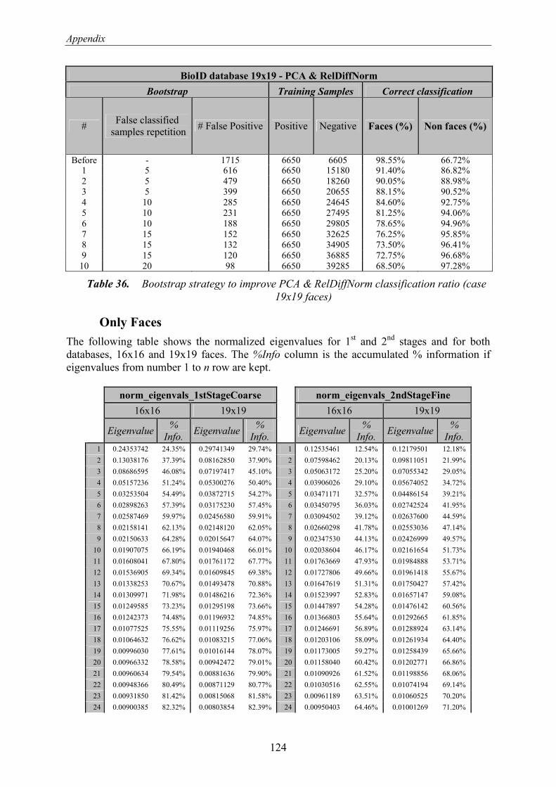
Appendix
124
BioID database 19x19 - PCA & RelDiffNorm
Bootstrap Training Samples Correct classification
# False classified
samples repetition # False Positive Positive Negative Faces (%) Non faces (%)
Before - 1715 6650 6605 98.55% 66.72% 1 5 616 6650 15180 91.40% 86.82%
2 5 479 6650 18260 90.05% 88.98% 3 5 399 6650 20655 88.15% 90.52%
4 10 285 6650 24645 84.60% 92.75% 5 10 231 6650 27495 81.25% 94.06%
6 10 188 6650 29805 78.65% 94.96%
7 15 152 6650 32625 76.25% 95.85% 8 15 132 6650 34905 73.50% 96.41%
9 15 120 6650 36885 72.75% 96.68% 10 20 98 6650 39285 68.50% 97.28%
Table 36. Bootstrap strategy to improve PCA & RelDiffNorm classification ratio (case
19x19 faces)
Only Faces
The following table shows the normalized eigenvalues for 1st and 2
nd stages and for both
databases, 16x16 and 19x19 faces. The %Info column is the accumulated % information if
eigenvalues from number 1 to n row are kept.
norm_eigenvals_1stStageCoarse norm_eigenvals_2ndStageFine
16x16 19x19 16x16 19x19
Eigenvalue %
Info. Eigenvalue
%
Info. Eigenvalue
%
Info. Eigenvalue
%
Info. 1 0.24353742 24.35% 0.29741349 29.74% 1 0.12535461 12.54% 0.12179501 12.18%
2 0.13038176 37.39% 0.08162850 37.90% 2 0.07598462 20.13% 0.09811051 21.99%
3 0.08686595 46.08% 0.07197417 45.10% 3 0.05063172 25.20% 0.07055342 29.05%
4 0.05157236 51.24% 0.05300276 50.40% 4 0.03906026 29.10% 0.05674052 34.72%
5 0.03253504 54.49% 0.03872715 54.27% 5 0.03471171 32.57% 0.04486154 39.21%
6 0.02898263 57.39% 0.03175230 57.45% 6 0.03450795 36.03% 0.02742524 41.95%
7 0.02587469 59.97% 0.02456580 59.91% 7 0.03094502 39.12% 0.02637600 44.59%
8 0.02158141 62.13% 0.02148120 62.05% 8 0.02660298 41.78% 0.02553036 47.14%
9 0.02150633 64.28% 0.02015647 64.07% 9 0.02347530 44.13% 0.02426999 49.57%
10 0.01907075 66.19% 0.01940468 66.01% 10 0.02038604 46.17% 0.02161654 51.73%
11 0.01608041 67.80% 0.01761172 67.77% 11 0.01763669 47.93% 0.01984888 53.71%
12 0.01536905 69.34% 0.01609845 69.38% 12 0.01727806 49.66% 0.01961418 55.67%
13 0.01338253 70.67% 0.01493478 70.88% 13 0.01647619 51.31% 0.01750427 57.42%
14 0.01309971 71.98% 0.01486216 72.36% 14 0.01523997 52.83% 0.01657147 59.08%
15 0.01249585 73.23% 0.01295198 73.66% 15 0.01447897 54.28% 0.01476142 60.56%
16 0.01242373 74.48% 0.01196932 74.85% 16 0.01366803 55.64% 0.01292665 61.85%
17 0.01077525 75.55% 0.01119256 75.97% 17 0.01246691 56.89% 0.01288924 63.14%
18 0.01064632 76.62% 0.01083215 77.06% 18 0.01203106 58.09% 0.01261934 64.40%
19 0.00996030 77.61% 0.01016144 78.07% 19 0.01173005 59.27% 0.01258439 65.66%
20 0.00966332 78.58% 0.00942472 79.01% 20 0.01158040 60.42% 0.01202771 66.86%
21 0.00960634 79.54% 0.00881636 79.90% 21 0.01090926 61.52% 0.01198856 68.06%
22 0.00948366 80.49% 0.00871129 80.77% 22 0.01030516 62.55% 0.01074194 69.14%
23 0.00931850 81.42% 0.00815068 81.58% 23 0.00961189 63.51% 0.01060525 70.20%
24 0.00900385 82.32% 0.00803854 82.39% 24 0.00950403 64.46% 0.01001269 71.20%

Appendix
125
25 0.00874649 83.20% 0.00766501 83.15% 25 0.00879985 65.34% 0.00965452 72.16%
26 0.00865047 84.06% 0.00723305 83.88% 26 0.00865356 66.20% 0.00906038 73.07%
27 0.00818064 84.88% 0.00712770 84.59% 27 0.00845531 67.05% 0.00879003 73.95%
28 0.00805734 85.69% 0.00706184 85.30% 28 0.00822124 67.87% 0.00869687 74.82%
29 0.00777323 86.46% 0.00685356 85.98% 29 0.00786503 68.66% 0.00864928 75.68%
30 0.00758397 87.22% 0.00684330 86.66% 30 0.00755500 69.41% 0.00846978 76.53%
31 0.00746809 87.97% 0.00650565 87.32% 31 0.00751580 70.16% 0.00804449 77.33%
32 0.00709702 88.68% 0.00638851 87.95% 32 0.00735088 70.90% 0.00747040 78.08%
33 0.00680969 89.36% 0.00612301 88.57% 33 0.00721965 71.62% 0.00717165 78.80%
34 0.00637637 90.00% 0.00600579 89.17% 34 0.00720880 72.34% 0.00694999 79.49%
35 0.00620387 90.62% 0.00594304 89.76% 35 0.00705804 73.05% 0.00682832 80.18%
36 0.00619757 91.24% 0.00590618 90.35% 36 0.00692655 73.74% 0.00647355 80.82%
37 0.00605538 91.84% 0.00575636 90.93% 37 0.00665413 74.41% 0.00621243 81.44%
38 0.00585918 92.43% 0.00556645 91.48% 38 0.00634823 75.04% 0.00612236 82.06%
39 0.00552127 92.98% 0.00551295 92.04% 39 0.00622386 75.66% 0.00591965 82.65%
40 0.00545338 93.53% 0.00538084 92.57% 40 0.00619481 76.28% 0.00573830 83.22%
41 0.00527897 94.05% 0.00525316 93.10% 41 0.00595773 76.88% 0.00565814 83.79%
42 0.00503820 94.56% 0.00508522 93.61% 42 0.00579434 77.46% 0.00526694 84.32%
43 0.00481770 95.04% 0.00494117 94.10% 43 0.00566498 78.02% 0.00506287 84.82%
44 0.00432901 95.47% 0.00488741 94.59% 44 0.00543237 78.57% 0.00471086 85.29%
45 0.00426101 95.90% 0.00484839 95.08% 45 0.00535854 79.10% 0.00463231 85.76%
46 0.00418303 96.32% 0.00476083 95.55% 46 0.00535320 79.64% 0.00453850 86.21%
47 0.00409667 96.73% 0.00467173 96.02% 47 0.00523636 80.16% 0.00426753 86.64%
48 0.00386853 97.11% 0.00443943 96.46% 48 0.00519859 80.68% 0.00420569 87.06%
49 0.00357816 97.47% 0.00440883 96.90% 49 0.00514256 81.20% 0.00395871 87.45%
50 0.00356541 97.83% 0.00432886 97.34% 50 0.00496768 81.69% 0.00395061 87.85%
51 0.00325301 98.15% 0.00412146 97.75% 51 0.00490638 82.18% 0.00371788 88.22%
52 0.00308699 98.46% 0.00387573 98.14% 52 0.00464763 82.65% 0.00363730 88.58%
53 0.00298577 98.76% 0.00353820 98.49% 53 0.00454663 83.10% 0.00355528 88.94%
54 0.00278570 99.04% 0.00348123 98.84% 54 0.00447461 83.55% 0.00348685 89.29%
55 0.00260892 99.30% 0.00321532 99.16% 55 0.00440652 83.99% 0.00342219 89.63%
56 0.00251061 99.55% 0.00304941 99.46% 56 0.00429981 84.42% 0.00335189 89.97%
57 0.00227481 99.78% 0.00275796 99.74% 57 0.00419875 84.84% 0.00323566 90.29%
58 0.00222639 100.00% 0.00259975 100.00% 58 0.00413507 85.25% 0.00320924 90.61%
59 0.00000000 100.00% 0.00000000 100.00% 59 0.00401268 85.66% 0.00318983 90.93%
60 0.00392479 86.05% 0.00299907 91.23%
61 0.00391857 86.44% 0.00297466 91.53%
62 0.00390397 86.83% 0.00279602 91.81%
63 0.00362503 87.19% 0.00277648 92.08%
64 0.00357767 87.55% 0.00269814 92.35%
65 0.00342822 87.89% 0.00256979 92.61%
66 0.00339517 88.23% 0.00253929 92.86%
67 0.00323549 88.56% 0.00247039 93.11%
68 0.00320742 88.88% 0.00244557 93.36%
69 0.00317632 89.20% 0.00239928 93.60%
70 0.00315771 89.51% 0.00231715 93.83%
71 0.00305668 89.82% 0.00222184 94.05%
72 0.00302072 90.12% 0.00217934 94.27%
73 0.00300564 90.42% 0.00194956 94.46%
74 0.00297712 90.72% 0.00192056 94.65%
75 0.00290602 91.01% 0.00190236 94.84%
76 0.00278255 91.29% 0.00184928 95.03%
77 0.00277422 91.56% 0.00184149 95.21%
78 0.00271203 91.83% 0.00177424 95.39%
79 0.00264234 92.10% 0.00176544 95.57%
80 0.00258579 92.36% 0.00167142 95.73%

Appendix
126
81 0.00257527 92.62% 0.00167010 95.90%
82 0.00248434 92.86% 0.00162258 96.06%
83 0.00247439 93.11% 0.00154356 96.22%
84 0.00239421 93.35% 0.00147870 96.37%
85 0.00231199 93.58% 0.00145658 96.51%
86 0.00228449 93.81% 0.00139190 96.65%
87 0.00220468 94.03% 0.00135088 96.79%
88 0.00216097 94.25% 0.00134025 96.92%
89 0.00213004 94.46% 0.00132940 97.05%
90 0.00209399 94.67% 0.00131632 97.18%
91 0.00202191 94.87% 0.00127480 97.31%
92 0.00201318 95.07% 0.00125149 97.44%
93 0.00192284 95.26% 0.00120773 97.56%
94 0.00190648 95.46% 0.00114775 97.67%
95 0.00189100 95.64% 0.00111585 97.78%
96 0.00185387 95.83% 0.00111239 97.90%
97 0.00181938 96.01% 0.00110587 98.01%
98 0.00175717 96.19% 0.00104420 98.11%
99 0.00171840 96.36% 0.00103750 98.21%
100 0.00169826 96.53% 0.00099337 98.31%
101 0.00168513 96.70% 0.00095946 98.41%
102 0.00159251 96.86% 0.00095299 98.51%
103 0.00148896 97.01% 0.00095090 98.60%
104 0.00148299 97.15% 0.00093801 98.69%
105 0.00140249 97.29% 0.00083023 98.78%
106 0.00139934 97.43% 0.00082190 98.86%
107 0.00135412 97.57% 0.00072448 98.93%
108 0.00133676 97.70% 0.00072258 99.00%
109 0.00131675 97.84% 0.00066984 99.07%
110 0.00130370 97.97% 0.00065563 99.14%
111 0.00126017 98.09% 0.00055989 99.19%
112 0.00125414 98.22% 0.00054890 99.25%
113 0.00121040 98.34% 0.00051210 99.30%
114 0.00119124 98.46% 0.00046783 99.35%
115 0.00115773 98.57% 0.00046374 99.39%
116 0.00111848 98.68% 0.00045062 99.44%
117 0.00109330 98.79% 0.00044689 99.48%
118 0.00104392 98.90% 0.00044337 99.53%
119 0.00097247 99.00% 0.00040027 99.57%
120 0.00092149 99.09% 0.00038846 99.60%
121 0.00087244 99.18% 0.00038544 99.64%
122 0.00086715 99.26% 0.00037030 99.68%
123 0.00083928 99.35% 0.00035805 99.72%
124 0.00074846 99.42% 0.00034957 99.75%
125 0.00072517 99.49% 0.00034225 99.79%
126 0.00068522 99.56% 0.00032488 99.82%
127 0.00065956 99.63% 0.00028246 99.85%
128 0.00059138 99.69% 0.00027660 99.87%
129 0.00058092 99.74% 0.00024553 99.90%
130 0.00056629 99.80% 0.00021736 99.92%
131 0.00051924 99.85% 0.00019889 99.94%
132 0.00043977 99.90% 0.00018680 99.96%
133 0.00040052 99.94% 0.00017359 99.98%
134 0.00035491 99.97% 0.00013062 99.99%

Appendix
127
135 0.00027124 100.00% 0.00011160 100.00%
136 0.00000000 100.00% 0.00000000 100.00%
137 0.00000000 100.00% 0.00000000 100.00%
138 0.00000000 100.00% 0.00000000 100.00%
139 0.00000000 100.00% 0.00000000 100.00%
140 0.00000000 100.00% 0.00000000 100.00%
141 0.00000000 100.00% 0.00000000 100.00%
142 0.00000000 100.00% 0.00000000 100.00%
143 0.00000000 100.00% 0.00000000 100.00%
144 0.00000000 100.00% 0.00000000 100.00%
Table 37. Face Detection: PCA only faces eigenvalues for both stages and DB
III.1.4. Support Vector Machine
The following table presents the classification result using SVM. Each row contains a
bootstrap iteration with the following information (from left to right):
• Current bootstrap iteration.
• Number of repetition of the false classified samples reintroduced in the training set.
• The number of non faces training samples incorrectly classified.
• Number of positive and negative training samples.
• Percentage of faces and non faces correctly classified.
GTAV database 16x16 - SVM
Bootstrap Training Samples Correct classification
# False Positive 1st Stage
Classification Ratio
2nd Stage (Final)
Classification Ratio #
False
classified
samples
repetition 1st
Stage
2nd
Stage
Positive Negative
Faces
(%)
Non faces
(%)
Faces
(%)
Non faces
(%)
before - 698 9 6650 6605 96.20% 86.861% 95.95% 99.525% 1 5 151 0 6650 10123 79.20% 95.996% 79.15% 99.863%
2 5 98 0 6650 10878 74.25% 97.316% 74.20% 99.907% 3 5 70 0 6650 11368 71.65% 97.751% 71.60% 99.912%
4 5 54 0 6650 11718 69.05% 98.078% 69.00% 99.926% 5 5 37 0 6650 11988 67.40% 98.237% 67.35% 99.929%
Table 38. Bootstrap strategy to improve SVM classification ratio (case 16x16 faces)
BioID database 19x19 - SVM
Bootstrap Training Samples Correct classification
# False Positive 1st Stage
Classification Ratio
2nd Stage (Final)
Classification Ratio #
False
classified
samples
repetition 1st
Stage
2nd
Stage
Positive Negative Faces
(%)
Non faces
(%)
Faces
(%)
Non faces
(%)
before - 357 10 6650 6605 94.40% 89.216% 94.40% 99.493% 1 5 124 0 6650 8390 76.10% 97.672% 75.65% 99.915%
2 5 50 0 6650 9010 64.60% 98.657% 64.20% 99.932% 3 5 28 0 6650 9260 56.55% 98.977% 56.15% 99.937%
4 5 14 0 6650 9400 48.80% 99.216% 48.45% 99.950% 5 5 7 0 6650 9470 43.30% 99.377% 43.00% 99.965%
Table 39. Bootstrap strategy to improve SVM classification ratio (case 19x19 faces)

Appendix
128
III.1.5. PCA & SVM
The following tables presents the classification result using PCA & SVM for the case of using
14 and 56 eigenvalues (1st and 2
nd stage) and the case of using 25 and 79 eigenvalues. Each
row contains a bootstrap iteration with the following information (from left to right):
• Current bootstrap iteration.
• Number of repetition of the false classified samples reintroduced in the training set.
• The number of non faces training samples incorrectly classified.
• Number of positive and negative training samples.
• Percentage of faces and non faces correctly classified.
GTAV database 16x16 - PCA (14_56) + SVM
Bootstrap Training Samples Correct classification
# False Positive 1st Stage
Classification Ratio
2nd Stage (Final)
Classification Ratio #
False
classified
samples
repetition 1st
Stage
2nd
Stage
Positive Negative Faces
(%)
Non faces
(%)
Faces
(%)
Non faces
(%)
before - 958 5 8171 6605 94.35% 81.333% 94.30% 99.097% 1 5 155 0 8171 11395 66.05% 95.269% 66.00% 99.748%
2 5 100 0 8171 12170 61.80% 96.767% 61.75% 99.824%
3 5 69 0 8171 12670 57.65% 97.491% 57.65% 99.857% 4 5 55 0 8171 13015 54.30% 97.965% 54.30% 99.890%
5 10 34 0 8171 13565 49.00% 98.582% 49.00% 99.924%
Table 40. Bootstrap strategy to improve PCA(14_56)+SVM classification ratio (case
16x16 faces)
GTAV database 16x16 - PCA (25_79) + SVM
Bootstrap Training Samples Correct classification
# False Positive 1st Stage
Classification Ratio
2nd Stage (Final)
Classification Ratio #
False
classified
samples
repetition 1st
Stage
2nd
Stage
Positive Negative Faces
(%)
Non faces
(%)
Faces
(%)
Non faces
(%)
before - 893 0 8171 6605 95.65% 83.030% 95.65% 99.301% 1 5 155 0 8171 11070 69.25% 95.710% 69.25% 99.806%
2 5 104 0 8171 11845 63.75% 97.117% 63.75% 99.854%
3 5 61 0 8171 12365 59.55% 97.883% 59.55% 99.899% 4 5 48 0 8171 12670 57.10% 98.154% 57.10% 99.918%
5 10 34 0 8171 13150 53.55% 98.448% 53.55% 99.934%
Table 41. Bootstrap strategy to improve PCA(25_79)+SVM classification ratio (case
16x16 faces)

Appendix
129
IV. Face Recognition Result
This section contains some detailed information that can help to understand face recognition
experimental results.
IV.1.1. Chi Square Dissimilarly Metric
In experimental results chapter, in section 7.3.1, results table show summarized information,
given the global ID recognition rate for each experiment. Following tables contains more
detailed information for each individual ID.
� Histogram equalization versus Mask using no Block Weight
Test 1 Test 2 Test 3 Test 4
Equalized Histogram x x � �
Mask x � x �
Blocks Weight x x x x
Type
Model 1 Img Mean 1 Img Mean 1 Img Mean 1 Img Mean Number ID
Samples ID# ID Recognition Rate %
216 ID1 55.09% 95.37% 54.63% 96.30% 55.09% 95.37% 53.70% 96.30%
120 ID2 70.00% 100.00% 60.83% 100.00% 70.83% 100.00% 60.00% 100.00%
194 ID3 45.36% 98.97% 42.27% 98.97% 47.42% 98.97% 43.30% 98.97%
80 ID4 63.75% 100.00% 62.50% 100.00% 63.75% 100.00% 62.50% 100.00%
198 ID5 40.40% 100.00% 37.88% 100.00% 39.90% 100.00% 37.37% 100.00%
4 ID6 100.00% 100.00% 100.00% 100.00% 100.00% 100.00% 100.00% 100.00%
118 ID7 27.12% 100.00% 27.12% 100.00% 27.12% 100.00% 27.12% 100.00%
156 ID8 71.15% 98.72% 71.79% 91.67% 71.79% 96.15% 71.79% 91.67%
176 ID9 28.98% 84.09% 30.68% 83.52% 29.55% 84.09% 30.68% 82.95%
176 ID10 96.02% 100.00% 92.61% 100.00% 97.73% 100.00% 93.18% 100.00%
122 ID11 49.18% 100.00% 49.18% 100.00% 49.18% 100.00% 49.18% 100.00%
142 ID12 44.37% 98.59% 45.77% 98.59% 44.37% 98.59% 45.07% 98.59%
212 ID13 44.81% 95.28% 41.04% 93.40% 44.34% 95.28% 41.51% 93.87%
298 ID14 76.85% 100.00% 69.13% 100.00% 77.85% 100.00% 71.14% 100.00%
188 ID15 37.23% 100.00% 35.11% 100.00% 37.23% 100.00% 34.57% 100.00%
100 ID16 96.00% 100.00% 99.00% 100.00% 96.00% 100.00% 99.00% 100.00%
102 ID17 58.82% 100.00% 57.84% 100.00% 58.82% 100.00% 57.84% 100.00%
70 ID18 44.29% 85.71% 40.00% 80.00% 42.86% 85.71% 38.57% 81.43%
80 ID19 50.00% 100.00% 50.00% 100.00% 51.25% 100.00% 50.00% 100.00%
12 ID20 50.00% 100.00% 58.33% 100.00% 50.00% 100.00% 58.33% 100.00%
92 ID21 100.00% 100.00% 98.91% 100.00% 100.00% 100.00% 98.91% 100.00%
102 ID22 50.00% 100.00% 54.90% 100.00% 50.98% 100.00% 52.94% 100.00%
50 ID23 94.00% 100.00% 100.00% 100.00% 98.00% 100.00% 100.00% 100.00%
57.48% 97.87% 55.75% 97.27% 57.95% 97.74% 55.78% 97.31%
77.67% 76.51% 77.84% 76.54%
Table 42. ID recognition rate (%) for each ID. Histogram equalization versus Mask

Appendix
130
� Histogram equalization versus Mask using Block Weight (1)
Test 5 Test 6 Test 7
Equalized Histogram x � �
Mask x x �
Blocks Weight �(1) �(1) �(1)
Type
Model 1 Img Mean 1 Img Mean 1 Img Mean Number ID
Samples ID# ID Recognition Rate %
216 ID1 59.72% 97.22% 61.11% 97.22% 62.04% 96.30%
120 ID2 76.67% 100.00% 76.67% 100.00% 76.67% 100.00%
194 ID3 30.93% 100.00% 30.93% 100.00% 29.38% 100.00%
80 ID4 81.25% 100.00% 82.50% 100.00% 82.50% 100.00%
198 ID5 46.46% 100.00% 45.96% 100.00% 47.47% 100.00%
4 ID6 100.00% 100.00% 100.00% 100.00% 100.00% 100.00%
118 ID7 28.81% 100.00% 27.97% 100.00% 25.42% 100.00%
156 ID8 83.33% 96.15% 83.33% 96.15% 83.33% 93.59%
176 ID9 43.18% 89.77% 43.75% 89.77% 42.61% 92.05%
176 ID10 97.16% 100.00% 98.30% 100.00% 98.30% 100.00%
122 ID11 67.21% 100.00% 67.21% 100.00% 68.03% 100.00%
142 ID12 48.59% 98.59% 48.59% 98.59% 47.18% 98.59%
212 ID13 54.72% 97.17% 53.77% 98.11% 50.94% 94.81%
298 ID14 77.18% 100.00% 79.19% 100.00% 76.85% 100.00%
188 ID15 45.74% 98.94% 45.74% 100.00% 45.21% 100.00%
100 ID16 93.00% 100.00% 92.00% 100.00% 89.00% 100.00%
102 ID17 60.78% 100.00% 60.78% 100.00% 60.78% 100.00%
70 ID18 38.57% 97.14% 38.57% 97.14% 37.14% 97.14%
80 ID19 53.75% 100.00% 53.75% 100.00% 53.75% 100.00%
12 ID20 83.33% 100.00% 83.33% 100.00% 83.33% 100.00%
92 ID21 98.91% 100.00% 98.91% 100.00% 98.91% 100.00%
102 ID22 74.51% 100.00% 73.53% 100.00% 71.57% 100.00%
50 ID23 100.00% 100.00% 100.00% 100.00% 100.00% 100.00%
62.76% 98.60% 63.00% 98.74% 62.20% 98.44%
80.68% 80.87% 80.32%
Table 43. ID recognition rate (%) for each ID. Histogram equalization vs Mask using
Block Weight (1)

Appendix
131
� Histogram equalization versus Mask using Block Weight (2)
Test 8 Test 9 Test 10
Equalized Histogram x � �
Mask x x �
Blocks Weight �(2) �(2) �(2)
Type
Model 1 Img Mean 1 Img Mean 1 Img Mean Number ID
Samples ID# ID Recognition Rate %
216 ID1 57.87% 97.22% 58.33% 97.22% 58.33% 97.22%
120 ID2 75.83% 100.00% 72.50% 100.00% 72.50% 100.00%
194 ID3 28.87% 97.94% 29.90% 97.94% 29.90% 97.94%
80 ID4 70.00% 100.00% 73.75% 100.00% 73.75% 100.00%
198 ID5 43.94% 97.98% 43.43% 97.98% 43.43% 97.98%
4 ID6 100.00% 100.00% 100.00% 100.00% 100.00% 100.00%
118 ID7 29.66% 98.31% 30.51% 98.31% 30.51% 98.31%
156 ID8 84.62% 80.77% 83.97% 80.77% 83.97% 80.77%
176 ID9 47.16% 90.91% 47.16% 88.64% 47.16% 88.64%
176 ID10 97.73% 100.00% 98.86% 100.00% 98.86% 100.00%
122 ID11 74.59% 100.00% 72.13% 100.00% 72.13% 100.00%
142 ID12 51.41% 98.59% 52.11% 98.59% 52.11% 98.59%
212 ID13 53.77% 95.28% 53.77% 95.28% 53.77% 95.28%
298 ID14 72.82% 100.00% 76.17% 100.00% 76.17% 100.00%
188 ID15 41.49% 98.94% 40.96% 98.94% 40.96% 98.94%
100 ID16 73.00% 100.00% 71.00% 100.00% 71.00% 100.00%
102 ID17 60.78% 100.00% 60.78% 100.00% 60.78% 100.00%
70 ID18 35.71% 94.29% 35.71% 97.14% 35.71% 97.14%
80 ID19 53.75% 100.00% 55.00% 100.00% 55.00% 100.00%
12 ID20 75.00% 100.00% 75.00% 100.00% 75.00% 100.00%
92 ID21 98.91% 100.00% 98.91% 100.00% 98.91% 100.00%
102 ID22 84.31% 100.00% 87.25% 100.00% 87.25% 100.00%
50 ID23 100.00% 100.00% 100.00% 100.00% 100.00% 100.00%
61.60% 97.34% 62.00% 97.27% 62.00% 97.27%
79.47% 79.63% 79.63%
Table 44. ID recognition rate (%) for each ID. Histogram equalization vs Mask using
Block Weight (2)

Appendix
132
V. OpenCV Functions Reference
OpenCV Library 1.0, Intel® Open Source Computer Vision Library (see [32][33]) is a
collection of C functions and a few C++ classes that implement many popular Image
Processing and Computer Vision algorithms.
Following section describes the most important OpenCV functions used in this research.
Principal Component Analysis
PCA algorithm is already implemented in the CxCore library of OpenCV and following
functions are the ones needed to perform Principal Component Analysis:
• cvCalcPCA: this function performs Principal Component Analysis of a given vector
set. First, cvCalcCovarMatrix is used to compute covariation matrix and its
eigenvalues and eigenvectors. The returned values are:
- Mean (average) vector.
- Output eigenvalues of covariation matrix.
- Output eigenvectors of covariation matrix (principal components).
• cvProjectPCA: this function projects input vectors to the specified subspace
represented by the orthonormal basis (eigenvectors). First of all, average vector is
subtracted from the input vectors. The returned value is:
- Output matrix of decomposition coefficients.
• cvBackProjectPCA: this function reconstructs the original vectors from the projection
coefficients. It is used only in case of using only faces class. The returned value is:
- The output matrix of reconstructed vectors.
Support Vector Machine
The implementation of SVM is available in the OpenCV’s Machine Learning Library (MLL),
a set of classes and functions for statistical classification, regression and clustering of data.
Due to the fact that it is an open source library, some modifications have been made in order
to get the score of the classification and not only the result face/non-face.
SVM parameters (CvSVMParams) definition:
• svm_type: Type of SVM, one of the following:
CvSVM::C_SVC - n-class classification (n≥2), allows imperfect separation of
classes with penalty multiplier C for outliers.
CvSVM::NU_SVC - n-class classification with possible imperfect separation.
Parameter nu is used instead of C. nu is in the range 0 to 1 and the larger the
value, the smoother the decision boundary.
CvSVM::ONE_CLASS - one-class SVM. All the training data are from the
same class, SVM builds a boundary that separates the class from the rest of the
feature space.

Appendix
133
CvSVM::EPS_SVR - regression. The distance between feature vectors from
the training set and the fitting hyperplane must be less than p. For outliers the
penalty multiplier C is used.
CvSVM::NU_SVR - regression. nu is used instead of p.
• kernel_type: The kernel type, one of the following:
CvSVM::LINEAR - no mapping is done, linear discrimination (or regression)
is done in the original feature space. It is the fastest option:
d(x,y) = x•y == (x,y) (1)
CvSVM::POLY - polynomial kernel:
d(x,y) = (gamma*(x•y)+coef0)degree
(2)
CvSVM::RBF - radial-basis-function kernel; a good choice in most cases:
d(x,y) = exp(-gamma*|x-y|2) (3)
CvSVM::SIGMOID - sigmoid function is used as a kernel:
d(x,y) = tanh(gamma*(x•y)+coef0) (4)
• degree, gamma, coef0: Parameters of the kernel, used in the formulas above.
• C, nu, p: Parameters in the generalized SVM optimization problem.
• class_weights: Optional weights, assigned to particular classes. They are multiplied
by C and thus affect the misclassification penalty for different classes. The larger the
weight is, the larger the penalty on misclassification of data from the corresponding
class is.
• term_crit: Termination procedure for iterative SVM training procedure, which solves
a partial case of constrained quadratic optimization problem. It stops either after a
certain number of iterations (term_crit.num_iter) or when the parameters change too
little (no more than term_crit.epsilon) from iteration to iteration.
In experimental results (see section 7.2.3), following SVM parameters are used:
svm_type CvSVM::C_SVC
kernel_type CvSVM::POLY
degree 2
gamma 1
coef0 1
C 5
term_crit only term_crit.epsilon with value 0.000000001
Table 45. SVM parameters using OpenCV Machine Learning Library
The epsilon termination criterion is empirically found as a trade off between computation
time and optimal results.
Skin Segmentation
Skin Segmentation procedure is implemented by means of OpenCV library image processing
algorithms.

Appendix
134
• Image preprocessing (training / test)
In image preprocessing step, the original image is smoothed to avoid compression noise and
other artifacts. Therefore, a 3x3 simple blur filter from OpenCV Library is used, consisting of
the sum over a pixel 3×3 neighborhood with subsequent scaling by 1/(3x3).
// image PRE processing
cvSmooth( ipl_Orig_RGB_Image, ipl_RGB_Image, CV_BLUR, 3, 3, 0, 0 );
• LUV conversion (training / test)
A function to perform LUV conversion and another one to split the 3 components are also
available in OpenCV library:
// calculate Luv
cvCvtColor( ipl_RGB_Image, ipl_Luv_Image, CV_RGB2Luv );
// split
cvSplit( ipl_Luv_Image, ipl_L_Image, ipl_u_Image, ipl_v_Image, NULL);
The function cvCvtColor converts input image from one color space to another. And the
parameter CV_RGB2Luv indicates that the transformation selected is from RGB to CIE LUV.
• Skin model definition (training)
After color conversion, for each pixel and taking into account a given neighborhood, u and v
components mean value are calculated by mean of the following OpenCV Library function:
// mean value u & v
cvAvgSdv( ipl_u_Image, &u_mean, &u_std_dev, NULL );
cvAvgSdv( ipl_v_Image, &v_mean, &v_std_dev, NULL );
The function cvAvgSdv calculates the average value and standard deviation of array elements.
• Skin segmentation (test)
Given an image to be segmented and after preprocessing and converting to LUV color space,
u and v components mean values are calculated as in training stage. Then, for each pixel and
taking into account a SkinDetBoxSize region (see equation (37)), the mean value is calculated
using above cvAvgSdv function.
Then, skin model thresholds are applied to determinate if the box region is skin or not
resulting in a skin mask, where some morphological operations need to be applied to
eliminate isolated pixels after each down-sampling step:
1st) Closing: using a 3x5 pixels ellipse structuring element.
// Create an elliptic structuring element
nSize=3;
IplConvKernel* structElem1 =
cvCreateStructuringElementEx( nSize+2, // columns
nSize, // rows
floor((nSize+2)/2.0), // anchor_x
floor(nSize/2.0), // anchor_y
CV_SHAPE_ELLIPSE, // shape
NULL); // CV_SHAPE_CUSTOM values

Appendix
135
// Perform advanced morphological transformations - CLOSING
cvMorphologyEx( iplSkinMask, // source
iplSkinMask, // destination
NULL, // temporary image (not required)
structElem2, // structuring element
CV_MOP_ CLOSE, // morphological operation closing
1); // number of iterations
2nd
) Opening: using a 11 pixels radius circle structuring element.
// Create a circular structuring element
nSize=11;
IplConvKernel* structElem2 =
cvCreateStructuringElementEx( nSize, // columns
nSize, // rows
floor(nSize/2.0), // anchor_x
floor(nSize/2.0), // anchor_y
CV_SHAPE_ELLIPSE, // shape
NULL); // CV_SHAPE_CUSTOM values
// Perform advanced morphological transformations - OPENING
cvMorphologyEx( iplSkinMask, // source
iplSkinMask, // destination
NULL, // temporary image (not required)
structElem2, // structuring element
CV_MOP_OPEN, // morphological operation opening
1); // number of iterations

Acronyms & Abbreviations List
136
Acronyms & Abbreviations List
ASA American Standards Association
DB Database
CIE International Commission on Illumination (abbreviated French name)
CMU Carnegie Mellon University
DARPA Defense Advanced Research Products Agency
EPFL Ecole Polytechnique Fédérale de Lausanne
FERET Face Recognition Technology
FGNET Face and Gesture Recognition Working Group
GIF Graphics Interchange Format
GTAV Audio Visual Technologies Group (abbreviated Catalan name)
GUI Graphical User Interface
HSV color space (Hue, Saturation, Value)
JPEG Joint Photographic Experts Group
KLT Karhunen-Loéve Transform
LBP Local Binary Patterns
MATLAB Matrix Laboratory (Mathworks, Inc.)
MIT Massachusetts Institute of Technology
MLL Machine Learning Library
OpenCV Open Source Computer Vision
RelDiffNorm Relative Difference Normalized
PBM Portable Bit Map
PCA Principal Component Analysis
PGM Portable Gray Map
RGB color space (Red, Green, Blue)
ROI Region Of Interest
SVM Support Vector Machine
UCS Uniform Chromaticity Scale
UPC Universitat Politècnica de Catalunya

Bibliography
137
Bibliography
Publications:
[1] T.Ahonen, A.Hadid & M.Pietikäinen, Face Description with Local Binary Patterns:
Application to Face Recognition. Draft, 5th June 2006.
[2] A.Hadid, M.Heikkilä, T.Ahonen & M.Pietikäinen. A Novel Approach to Access
Control based on Face Recognition. Machine Vision Group, InfoTech Oulu and
Department of Electrical and Information Engineering. University of Oulu, Finland.
[3] T.Ahonen, M.Pietikäinen, A.Hadid & T.Mäenpaä. Face Recognition Based on the
Appearance of Local Regions. Machine Vision Group, InfoTech. University of Oulu,
Finland. 2004 IEEE.
[4] T.Ahonen, A.Hadid & M.Pietikäinen. Face Recognition with Local Binary Patterns.
Machine Vision Group, InfoTech. University of Oulu, Finland. T.Pajdla and J.Matas
(Eds): ECCV 2004, LNCS 3021, pp.469-481, 2004. Spring-Verlag Berlin Heidelberg
2004.
[5] A.Hadid & M.Pietikäinen. A Hybrid Approach to Face Detection under
Unconstrained Environments. Machine Vision Group, Dept. of Electrical and
Information Engineering. University of Oulu, Finland.
[6] A.Hadid, M.Pietikäinen & T.Ahonen. A Discriminative Feature Space for Detecting
and Recognizing Faces. Machine Vision Group, InfoTech Oulu and Dept. of Electrical
and Information Engineering. University of Oulu, Finland.
[7] T.Ojala, M.Pietikäinen & T.Mäenpaä. Multiresolution gray-scale and rotation
invariant texture classification with Local Binary Patterns. IEEE Transactions on
Pattern Analysis and Machine Intelligence, vol. 24, no. 7, pp. 971-987, July 2002.
[8] G.Heusch, Y.Rodriguez & S.Marcel. Local Binary Patterns as an Image
Preprocessing for Face Authentication. IDIAP Research Institute, Martigny,
Switzerland. Ecole Polytechnique Fédérale de Lausanne (EPFL), Switzerland.
[9] Y.Rodriguez & S.Marcel. Face Authentication using Adapted Local Binary Pattern
Histograms. IDIAP Research Institute, Martigny, Switzerland.
[10] S.Marcel, Y.Rodriguez & G.Heusch. On the Recent Use of Local Binary Patterns for
Face Authentication. IDIAP Research Institute, Martigny, Switzerland. International
Journal of Image and Video Processing, Special Issue on Facial Image Processing.
May 2007.
[11] E.Osuna, R.Freund & F.Girosi. Training Support Vector Machine: an Application to
Face Detection. In Proc. Computer Vision and Pattern Recognition, pages 130-136,
June 1997.
[12] Josep R. Casas, F. Marqués & P.Salembier. Apunts de l’assignatura: Processament
d’Imatge. Image Processing Group, Signal Theory & Comm. Dept, UPC. Barcelona,
Fall 2004.
[13] Lindsay I Smith. A tutorial on Principal Components Analysis. February 26, 2002.
[14] K.-K. Sung, Learning and Example Selection for Object and Pattern Detection, PhD
thesis, MIT AI Lab, Jan. 1996. Available as AI Technical Report 1572.

Bibliography
138
[15] G.Yang & T.S.Huang. Human Face Detection in Complex Background, Pattern
Recognition, vol. 27, no. 1, pp. 53-63, 1994.
[16] K.C.Yow & R.Cipolla. Feature-based human face detection, Image and Vision
Computing, vol. 15, no. 9, pp. 713 – 735, 1997.
[17] A.L.Yuille, P.W.Hallinan & D.S.Cohen. Feature extraction from faces using
deformable templates, International Journal of Computer Vision vol. 8, no. 2, 99–111,
1992.
[18] P.Juell & R.Marsh. A hierarchical neural network for human face detection, Pattern
Recog. 29, 1996, 781–787.
[19] E.Viennet & F.Fogelman Soulié. Connectionist methods for human face processing, in
Face Recognition: From Theory to Application, Springer-Verlag, Berlin/New York,
1998.
[20] M.Schulze, K.Scheffler, & K.W.Omlin. Recognizing Facial Actions with Support
Vector Machines, In Proc. PRASA, pp. 93-96, 2002.
[21] L.R.Rabiner. A tutorial on Hidden Markov Models and Selected Applications in
Speech Recognition, Proceedings IEEE, vol. 77, no. 2, Feb 1989.
[22] M.A.Turk & A.P.Pentland. Face recognition using eigenfaces, Proceedings of the
IEEE Computer Society Conf. on Computer Vision and Pattern Recognition, pp. 586-
591, Maui, Hawaii 1991.
[23] B.Zarit, B.J.Super & F.Quek. Comparison of five color models in skin pixel
classification, ICCV’99 Int’l Workshop on Recognition, Analysis and Tracking of
Faces and Gestures in Real-Time Systems, pp. 58–63, Corfu, Greece, September 1999.
[24] P.Viola & M.Jones. Rapid Object Detection using a Boosted Cascade of Simple
Features, Computer Vision and Pattern Recognition, 2001.
[25] C.H.Lee, J.S.Kim & K.H.Park. Automatic human face location in a complex
background, Pattern Recognition Letters, 29, 1877–1889, 1996.
[26] R.J.Qian, M.I.Sezan & K.E.Matthews. A Robust Real-Time Face Tracking Algorithm,
ICIP (1) 1998: 131-135.
[27] M.Lades, J.C.Vorbruggen, J.Buhmann, J.Lange, C.von der Malsburg, R.P.Wurtz &
W.Konen. Distortion Invariant Object Recognition in the Dynamic Link Architecture
IEEE Transactions on Computers archive Volume 42 , Issue 3 Pages: 300 – 311.
1993.
[28] P.Sinha, B.Balas, Y.Ostrovsky, R.Russell. Face recognition by humans: 20 results all
computer vision researchers should know about. Proceedings of the IEEE, 94, 1948–
1962. 2006.
[29] M.S.Keil. “I Look in Your Eyes, Honey”: Internal Face Features Induce Spatial
Frequency Preference for Human Face Processing. PLoS Computational Biology 5(3):
e1000329. doi:10.1371/journal.pcbi.1000329. 2009
Books:
[30] Richard O. Duda, Peter E.Hart, David Stork. Pattern Classification, 2nd
Edition Wiley.

Bibliography
139
[31] Joan Cabestany, Sergio Bermejo. Sistemas conexionistas para el tratamiento de la
información, Edicions UPC, Barcelona 2003.
Reference Manuals:
[32] Intel® Open Source Computer Vision Library. CXCORE, CV, Machine Learning and
HighGUI Reference Manuals, Intel Corporation. PDF Files (2006).
Web Pages:
[33] http://opencvlibrary.sourceforge.net: OpenCV Wiki-pages
[34] http://tech.groups.yahoo.com/group/OpenCV/: OpenCV Open Source Computer
Vision Library Community
[35] http://citeseer.ist.psu.edu/burges98tutorial.html: A Tutorial on Support Vector
Machines for Pattern Recognition - Burges (ResearchIndex)
[36] http://www.ee.oulu.fi/mvg/page/publications: University of Oulu - Machine Vision
Group
[37] http://www.ee.oulu.fi/research/imag/texture/lbp/about/LBP%20Methodology.pdf: University
of Oulu - LBP methodology
[38] http://www.humanscan.de/support/downloads/facedb.php : The BioID Face Database
[39] http://www.ysbl.york.ac.uk/~garib/mres_course/2005/Lecture5.ppt: Resampling
techniques.
[40] http://www.cs.cmu.edu/~awm/tutorials: Support Vector Machines tutorial by Andrew
W. Moore.
[41] http://www.svms.org/: Support Vector Machines (SVMs) web site.
[42] http://gps-tsc.upc.es/GTAV/: Audio Visual Technologies Group of the Signal Theory
and Communications Department of the Technical University of Catalonia.
[43] http://gps-tsc.upc.es/GTAV/ResearchAreas/UPCFaceDatabase/GTAVFaceDatabase.htm:
Audio Visual Technologies Group Face Database.
[44] http://www.ee.oulu.fi/mvg/page/lbp_matlab: University of Oulu - New LBP Matlab
implementation


![Remote Sensing Image Scene Classification Using Multi ... · 2.1. Completed Local Binary Patterns Local binary patterns (LBP) [21,22] are an effective measure of spatial structure](https://static.fdocuments.net/doc/165x107/5f0ce0fd7e708231d4379522/remote-sensing-image-scene-classification-using-multi-21-completed-local-binary.jpg)