Bachelor Informatica

License plate recognitionusingLocal Binary Patterns

Jayke Meijer, 6049885

June 11, 2012

Supervisor(s): Rein van den Boomgaard

Signed:

Informatica—

Universiteit

vanAmst

erdam

2

Abstract

In this work the efficiency of Local Binary Patterns as feature extraction method for characterrecognition in license plate images is tested. Several patterns and different classifiers are com-pared for both accuracy and speed. The ability to determine whether the given classification iscorrect is tested as well. The experiments show that it is effective in recognizing the charactersand the recognition is done in a short amount of time. The confidence of the classifier in thegiven answers proves not to be as good as hoped, but the system can still be used in real lifeapplications.

2

Contents

1 Introduction 5

1.1 Problem outline . . . . . . . . . . . . . . . . . . . . . . . . . . . . . . . . . . . . . 5

1.2 Goal of the investigation . . . . . . . . . . . . . . . . . . . . . . . . . . . . . . . . 5

1.3 Tasks to be performed . . . . . . . . . . . . . . . . . . . . . . . . . . . . . . . . . 6

2 Related work 7

2.1 Neural networks . . . . . . . . . . . . . . . . . . . . . . . . . . . . . . . . . . . . 7

2.2 SVM . . . . . . . . . . . . . . . . . . . . . . . . . . . . . . . . . . . . . . . . . . . 7

3 License plate recognition with LBPs 9

3.1 Earlier research of LBPs . . . . . . . . . . . . . . . . . . . . . . . . . . . . . . . . 9

3.2 Method . . . . . . . . . . . . . . . . . . . . . . . . . . . . . . . . . . . . . . . . . 9

3.3 Local Binary Patterns . . . . . . . . . . . . . . . . . . . . . . . . . . . . . . . . . 10

3.4 The different patterns tested . . . . . . . . . . . . . . . . . . . . . . . . . . . . . 11

3.5 Classifiers . . . . . . . . . . . . . . . . . . . . . . . . . . . . . . . . . . . . . . . . 13

4 Experiments 15

4.1 Method . . . . . . . . . . . . . . . . . . . . . . . . . . . . . . . . . . . . . . . . . 15

4.2 Testing setup . . . . . . . . . . . . . . . . . . . . . . . . . . . . . . . . . . . . . . 15

4.3 Accuracy . . . . . . . . . . . . . . . . . . . . . . . . . . . . . . . . . . . . . . . . 16

4.4 Speed . . . . . . . . . . . . . . . . . . . . . . . . . . . . . . . . . . . . . . . . . . 16

4.5 Confidence . . . . . . . . . . . . . . . . . . . . . . . . . . . . . . . . . . . . . . . 17

4.6 Special Patterns . . . . . . . . . . . . . . . . . . . . . . . . . . . . . . . . . . . . 19

5 Conclusion 21

5.1 Accuracy . . . . . . . . . . . . . . . . . . . . . . . . . . . . . . . . . . . . . . . . 21

5.2 Speed . . . . . . . . . . . . . . . . . . . . . . . . . . . . . . . . . . . . . . . . . . 22

5.3 Confidence . . . . . . . . . . . . . . . . . . . . . . . . . . . . . . . . . . . . . . . 23

5.4 Usability in real-life systems . . . . . . . . . . . . . . . . . . . . . . . . . . . . . . 23

5.5 Future work . . . . . . . . . . . . . . . . . . . . . . . . . . . . . . . . . . . . . . . 24

A Confusion Matrix 29

B Misclassified characters 31

C LIBSVM with C++ 33

3

4

CHAPTER 1

Introduction

1.1 Problem outline

Automatic License Plate Recognition is the field of technology that is used to read a license platein images. It is used in a number of different domains, such as parking systems but also by lawenforcement or toll roads.

ALPR is gaining popularity. Increasing numbers of police vehicles are equipped with mobilesystems. Simultaneously, more and more companies make the decision for a parking systemwhich uses ALPR. This is more convenient than traditional systems, since there is no actionrequired by the user such as inserting a key card.

1.2 Goal of the investigation

On simple devices, it is important to find a method that is faster than current systems, since theseare often too slow. This research focusses on the use of Local Binary Patterns and determines ifthis method is capable of correctly classifying a character on a license plate in a small amountof time.

The work described here is based on preliminary work performed by me and a number ofothers during the Computer Vision course at the University of Amsterdam [15]. In this inves-tigation it was shown that the use of LBPs is theoretically a good method for the classificationof characters. The report also suggested a number of improvements to the used method. Thesesuggestions are used in this research.

ALPR consists of six different steps [1]. These steps are as follows:

1. License Plate Localization

2. License Plate Sizing and Orientation

3. Normalization

4. Character Segmentation

5. Optical Character Recognition

6. Syntactical/geometrical analysis

This research is about the fifth step, the recognition of the separate characters.The research question is:“How efficient is the use of Local Binary Patterns for Automatic License Plate

Recognition?”The following sub-questions can be distinguished:

5

“How well can a single character of a license plate be recognized?” It is important to be able torecognize the characters on the license plate. This is the most important characteristic of thesystem.

To test this, a large number of images of characters will be classified by the program. Theclassification by the system is compared to the real character. The number of correctly classifiedcharacters can be expressed as a percentage of the total number of characters. The goal is to getthis percentage as high as possible.

“How fast can a single character of a license plate be recognized?” The recognition needs to bedone fast. Given the fact that there is more than one character on a license plate, the timeneeded per character is only a fraction of the total time available for the plate. It is thereforeimportant to optimize the speed of the algorithm as much as possible.

To test this speed, the time needed for recognition will be measured over a large set ofcharacters. By dividing this time by the number of characters tested, an average time percharacter can be determined.

How confident is the system about its answer? It is not only important that the classification isright in most cases, it is also important to know when the classification is wrong. Therefore, theconfidence of the given answer will be determined.

To visualise this data it is placed in a Receiver Operating Characteristic curve. This curveshows how many answers are correct when a certain rate of false positives is allowed. The curvewill be generated for the best performing system.

Application

This research is performed to be used in a new ALPR system for a company called Parkingware[2]. Parkingware develops automated systems for parking lots. The company is considered aworldwide market leader in this field.

1.3 Tasks to be performed

The following tasks need to be performed:

• Write the software in C++, based on a preliminary prototype written in Python[15].

• Implement and test different classifiers.

• Test the system with different parameter settings.

• Look into possibilities to use the classification system for license plate segmentation.

6

CHAPTER 2

Related work

Automatic license plate recognition is used in many different field. In each of these fields, there isan increasing interest in such systems. This leads to many different studies and therefore manydifferent types of systems. A number of these investigations will be discussed in this chapter.

2.1 Neural networks

Many researches use neural networks to classify the characters. For instance, Ondrej Martinsky[12] has designed a method that describes the local spacial structure, like the LBP system usedin this research, but as a classifier several types of neural networks are tested.

Before applying this method, many image preprocessing steps are performed to create abitmap of the image. The method described in our research does not need these steps since thedescriptor is not made based on a bitmap version of the image. The preprocessing steps usedmay lead to long calculation times. These times are not discussed by the author. There is alsono accuracy data available for the character recognition step only, so no comparison can be madewith the method proposed in our research.

Another research utilizing neural networks is performed by Kwasnicka and Wawrzyniak [8].For the feature extraction the vertical projection retrieved during segmentation is used. Theaccuracy of this method is 65% per license plate.

Lazrus and Choubey[9] use neural networks for several steps of ALPR. It is not clear whichdescriptor is used for the image. The accuracy of the entire system is 98% according to theauthor.

In another research the binary image of the character is used as input for the neural networkby Koval et al.[7]. An accuracy of 95% per character is achieved with this method, even whenintroducing an artificial salt and pepper noise with a density of 50%.

The last two methods shown both require a large amount of preprocessing on the image,which could increase the time needed for the recognition. This is not mentioned in the articles.

2.2 SVM

There are also applications that use a Support Vector Machine(SVM), which is one of the clas-sifiers in this research, but with a different method. Li[10] uses the SVM with a Histogram ofOriented Gradients or HOG descriptor for the feature extraction. This is further discussed insection 3.1.

7

8

CHAPTER 3

License plate recognition with LBPs

3.1 Earlier research of LBPs

The use of LBPs for license plate recognition has been researched before. Li[10] tries to use LBPsbefore the making the choice to use Histogram of Oriented Gradients or HOGs. However, thisdecision was based mainly on the results obtained for license plate localisation. The performanceof LBPs was not good enough for this task. The author wanted to use the same algorithm forevery step in his method, which is why he used HOGs for the character recognition as well.The HOG-based algorithm was not suited for this task, and his recommendation was to use atraditional OCR instead.

Liu et al[11] use LBPs succesfully for license plate recognition. The authors used a simplifiedform of the LBP and a slightly more advanced classifier than the maximum log-likelihood usedin the original LBP article[13], the Mahalanobis distance. They scored high recognition rates.This simplified pattern will therefore be implemented and tested.

3.2 Method

The implementation of a License Plate Recognizer using LBPs compromises a number of steps.Once an image file is read, it has to be preprocessed before it can be turned in a feature vector.The feature vector is then provided to the classifier, which determines the character displayed inthe image.

Preprocessing

The preprocessing of the image consists of two steps. The first step is to resize the imageto a standard size. The second step is to blur the image to remove noise. The result of thepreprocessing is shown in figure 3.1.

Rescaling The image is resized to a standardized height. The aspect-ratio is preserved. If thisratio changes, the spacial characteristics of the character change. This changes the descriptor ofthe image and affects the recognition.

Figure 3.1: Difference between the input image (left) and the image after preprocessing. Theimage is scaled and a Gaussian blur is applied to remove noise.

9

The scaling factor is based on the height because a license plate has a standard height, whichmeans the characters have a standard height as well. By using the height as standard eachcharacter in the system will have a size that is proportional to the others. Using the width forthis purpose would be wrong, since the characters have a different width. For example, a W iswider than an I.

For the rescaling, OpenCV’s resize() function is used, with a bilinear interpolation.

Filtering Noise is an important factor in the system. Noise is in this case any imperfection onthe license plate. This also includes dirt and the screws used to mount the plate to the vehicle.In order to suppress this noise as much as possible, a Gaussian Blur is applied. The scale or σof the blur applied is 1.9. This blur was found to be the best in [15].

The theory explained still applies. In the rescaled image, the width of a stroke is 8 to 10pixels. The width of the filter is 6 ∗ σ = 6 ∗ 1.9 = 11.4. Since this is slightly wider than thestroke, the stroke will be preserved in the image, but any smaller noise will be filtered.

The filtering is performed by the function GaussianBlur from OpenCV.

Feature extraction

Once the image has been preprocessed, a feature vector of the image can be created. This is doneby the Local Binary Pattern algorithm. First the image is separated in cells. Then, for each ofthese cells a histogram of found patterns is created. Finally, these histograms are concatenatedto form the descriptor for this image.

Cells The image is divided into cells. The number of cells in horizontal and vertical directionis a parameter for the entire system and as such is flexible.

The reason to work with cells is to introduce a form of locality. It is no longer possible tohave two characters which have the same patterns, but a different location of these patterns. Forexample, Consider the characters T and L. When only one cell is used, the histograms of thesecharacters have a large overlap, in the form of a horizontal and a vertical line. By using cellsthis is prevented.

This creates a trade-off. A high amount of cells will create a more precise description of thecharacter, but will require each character to be segmented more precisely, since the chance of akey feature being located in a different cell is higher, decreasing the translational invariance ofthe system.

Histogram creation For every cell a histogram is created. This is done by calculating a valuefor each pixel in the cell. This value describes the local spacial structure of the image aroundthe pixel. The value is determined by the Local Binary Pattern. How this value is calculated isdescribed in section 3.3.

The histogram of these values is used as a feature vector describing this cell.

Classification

Once the feature vector is available a classifier can be used to determine what character itrepresents. Several classifiers will be tested. The classifier will determine its most likely classand, if available, indicate how certain it is that the answer is right.

3.3 Local Binary Patterns

For each pixel the Local Binary Pattern is determined. This is a value that describes the localspacial structure. It is expressed as an integer value.

10

Calculation of LBP

To calculate the LBP for each pixel, its gray-scale value is compared to a number of pixels in theneighbourhood. These pixels are determined by the type of pattern used. The different patternsare discussed later on in this paper.

A comparison between the center pixel and one of the surrounding pixels gives either a 1 ora 0, indicating whether the center pixel has a higher gray-scale value. By comparing each of thesurrounding pixels, a bit-string can be created. This way, each unique spacial structure has itsown identifying value. Mathematically, the following equations from the original LBP article[13]describe the calculation of this value.

s(x) =

{1, x ≥ 00, x < 0

(3.1)

value =

P−1∑p=0

s(gp − gc)2p. (3.2)

In these equations gc is the gray-scale value of the center pixel and gp for p = 0, ..., P − 1 are thegray-scale values of the surrounding pixels.

Comparison with other local structure methods

There are other methods that create a description of the local spacial structure. One of suchmethods is the Histogram of Oriented Gradients or HOG[5]. The HOG algorithm is comparablein its use of cells and histograms. The difference is that it determines the gradient of the edgesfor a given area around a pixel instead of the actual spacial structure.

The HOG feature is capable of describing several directions of different lines at a certainpoint, by using the gradients magnitude as the function for the weighted vote. This makes it astrong classifier in images displaying natural content. However, license plates only have simpleedges, going in one direction at a time. This type of edges can be properly described by LocalBinary Patterns. That the HOG is not a good descriptor is experienced by Li[10]. He uses aHOG descriptor is for license plate recognition. The author concludes that it is not well suitedfor the task.

3.4 The different patterns tested

Local Binary Patterns can be determined in different shapes by using other neighbourhood pixelsto compare to. Several of these shapes will be tested. The following naming convention is usedfor these patterns: LBP riuX

P,R . In this convention, P stands for the number of points used andR stands for the radius of the circle these points are placed on. ri means that the pattern isrotation invariant and uX indicates that only uniform patterns are used, in which uniform meansthat there are a maximum of X transitions between 1 and 0 or vice versa.

LBP8,1

There are a number of different LBPs that will be tested. The first pattern is the most basic,called LBP8,1. The pattern uses the points shown in figure 3.2.

LBP8,(4/5/6)

Another pattern tested is LBP8,5. This pattern uses the same points as LBP8,1, but instead ofbeing next to the center pixel, they are further away. Note that this is not exactly as the LBPtheory specifies, since the theory specifies that a real circle should be used. However, that isto achieve rotational invariance. For this application the images are transformed to a standardorientation, which makes rotational invariance a useless feature for this implementation. Thismeans the simplified version can be used. Whether this assumption is correct will be tested.

11

Figure 3.2: Graphical representation of LBP8,1. The green pixels are compared to the red one,creating a bitstring and thus a value that identifies the spacial structure around this pixel.

Figure 3.3: Graphical representation of LBP8,5. The green pixels are compared to the red one,creating a bitstring and thus a value that identifies the spacial structure around this pixel.

The choice of radius 5 was based on early testing, but is theoretically explainable. The widthof a single stroke in a normalized character is about 8 to 10 pixels. By choosing the width ofthe pattern such that it hits both edges, the pattern will be able to describe the direction of thestroke properly. In order to verify this, testing is also performed with radii 4 and 6.

The pattern is shown in figure 3.3.

LBP u28,1

Another pattern that is tested is the LBPu28,1. This means that every pattern with more than

two transitions from 0 to 1 and 1 to 0 is placed in a single category. For instance, 00001110is a uniform pattern, since it only has two transitions. 00111001, however, is not, since thereare four transitions. The reason for using this type of pattern is explained by Ojala et al. [13].Patterns with more than two transitions are such a small portion of the total patterns, that theirprobabilities can not be estimated reliably.

The pixels used for the comparison are the same as those used in LBP8,1 and are thereforeshown in 3.2.

During the experiments it became clear that the (8, 4) version of this pattern was interestingto test as well. More on this in the experiments chapter.

LBP3,1

The final pattern to test is the pattern LBP3,1. This is what is called the S-LBP, and is introducedby Liu et al.[11]. Only three points are used. These points are not variable and have beenexperimentally determined by the authors. The results achieved were very promising. Thepoints used are shown in figure 3.4.

Figure 3.4: Graphical representation of LBP3,1. The green pixels are compared to the red one,creating a bitstring and thus a value that identifies the spacial structure around this pixel.

12

3.5 Classifiers

Maximum Log-likelihood

In the original LBP research[13] the maximum log-likelihood classifier is used. This is the firstclassifier tested. It is based of the log-likelihood ratio statistic. The formula for this ratio is givenin the article:

G(S,M) = 2

B∑b=1

Sb logSb

Mb= 2

B∑b=1

[Sb logSb − Sb logMb] (3.3)

In this equation, S stands for the vector of the sample used and M stands for the vector of thetrained model. The comparison is then performed between each feature of these vectors, whichare the bins of the histograms.

The formula used in the code is a simplification of (3.3):

L(S,M) =

B∑b=1

Sb logMb (3.4)

This simplification can be made since the term Sb logSb will be constant for each comparisonwith the stored classes and is therefore not relevant in the comparison of all the models with thesample.

Once L is known for each class, the class with the highest value for L is chosen as the bestmatching class.

The training of this classifier is done by calculating the average vector for the examples ofeach class.

Support Vector Machine

Currently, one of the most used classifiers is the Support Vector Machine. The current incarnationof this classifier was given by Corinna Cortes and Vladimir Vapnik in [4].

Since Support Vector Machines are often used in pattern recognition tasks, the expectation isthat it will perform well for the LBP descriptor. The speed with which the classification can beperformed is more interesting, since the SVM is a fairly advanced and complex method, whichmight show a less satisfying performance in very high dimensions.

Used implementation The SVM used is LIBSVM [3], a SVM written in C++ (a Java versionis available too), but with bindings for Python and a lot of other programming languages andenvironments. However, using this classifier in C++ is not straightforward and an explanationon how this should be done is provided as appendix C for future use.

Kernel and parameters The SVM requires the choice of a kernel. The most often used kernel isthe Radial Basis Function. For this reason, the RBF kernel is used for the experiments, sincethe chances of good results are the highest with this kernel. A linear kernel will also be tested,which is more simple, and therefore faster. If the dimension of the feature vector is high, a linearkernel might be as accurate as the RBF kernel [16].

The SVM has a parameter C, which defines the soft margin, i.e. it determines how manytraining examples are allowed to be located on the wrong side of the classification plane. For theRBF, there is a parameter γ in addition to C. γ Determines the shape of the radial kernel andtherefore the amount of transformation applied to the vector space when lifting it to a higherdimension.

Training For training the SVM, the training data is converted to a SVM data file. This datasetis scaled and used as input for the script easy.py provided in LIBSVM. This script performs agrid search to find parameters C and γ. After the best parameters have been determined, a SVMmodel is trained with the scaled data and the found parameters.

13

14

CHAPTER 4

Experiments

There are three main characteristics to be tested. The first characteristic is the recognitionrate or accuracy, which indicates the percentage of characters properly identified. The secondcharacteristic is the time in which the recognition is performed. The third characteristic is theability of the classifier to determine whether the recognized character is correct. Each will bediscussed separately.

4.1 Method

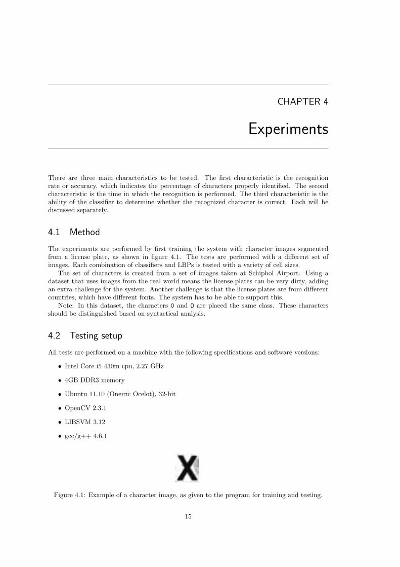
The experiments are performed by first training the system with character images segmentedfrom a license plate, as shown in figure 4.1. The tests are performed with a different set ofimages. Each combination of classifiers and LBPs is tested with a variety of cell sizes.

The set of characters is created from a set of images taken at Schiphol Airport. Using adataset that uses images from the real world means the license plates can be very dirty, addingan extra challenge for the system. Another challenge is that the license plates are from differentcountries, which have different fonts. The system has to be able to support this.

Note: In this dataset, the characters 0 and O are placed the same class. These charactersshould be distinguished based on syntactical analysis.

4.2 Testing setup

All tests are performed on a machine with the following specifications and software versions:

• Intel Core i5 430m cpu, 2.27 GHz

• 4GB DDR3 memory

• Ubuntu 11.10 (Oneiric Ocelot), 32-bit

• OpenCV 2.3.1

• LIBSVM 3.12

• gcc/g++ 4.6.1

Figure 4.1: Example of a character image, as given to the program for training and testing.

15

Table 4.1: The accuracy results for the maximum log-likelihood classifier. The vertical axisstates the number and distribution of cells, the horizontal axis the used LBP. The values are thepercentage of correctly classified characters.

LBP8,1 LBP8,4 LBP8,5 LBP8,6 LBP3,1 LBPu28,1

1x1 32.3 63.8 73.1 78.8 0.0 28.11x2 49.9 73.1 78.4 82.3 1.4 46.62x2 74.3 82.4 83.7 85.1 27.8 75.02x3 79.3 82.6 84.1 84.6 59.0 80.33x3 79.9 81.7 81.4 82.1 67.0 81.24x4 80.7 78.5 77.1 77.0 75.2 82.75x5 76.5 71.3 70.4 70.4 77.2 79.3

Table 4.2: The accuracy results for the Support Vector Machine classifier. The vertical axisstates the number and distribution of cells, the horizontal axis the used LBP. The values are thepercentage of correctly classified characters.

LBP8,1 LBP8,4 LBP8,5 LBP8,6 LBP3,1 LBPu28,1

1x1 86.5 96.7 97.2 98.1 3.7 49.81x2 92.0 97.5 97.7 98.1 4.3 89.32x2 95.7 98.5 98.1 98.3 89.5 96.22x3 97.2 98.4 98.6 98.6 93.5 96.93x3 96.9 98.2 98.6 98.3 94.0 97.24x4 97.1 98.7 98.7 98.3 95.0 97.45x5 97.0 97.7 98.1 97.9 95.6 97.2

4.3 Accuracy

The first characteristic is the accuracy. This is the main focus of the research, since a quickrecognition has no use if it is not accurate.

Maximum log-likelihood classifier

Table 4.1 contains the accuracy results for the maximum log-likelihood classifier.

Support Vector Machine

Table 4.2 contains the accuracy results for the Support Vector Machine classifier.

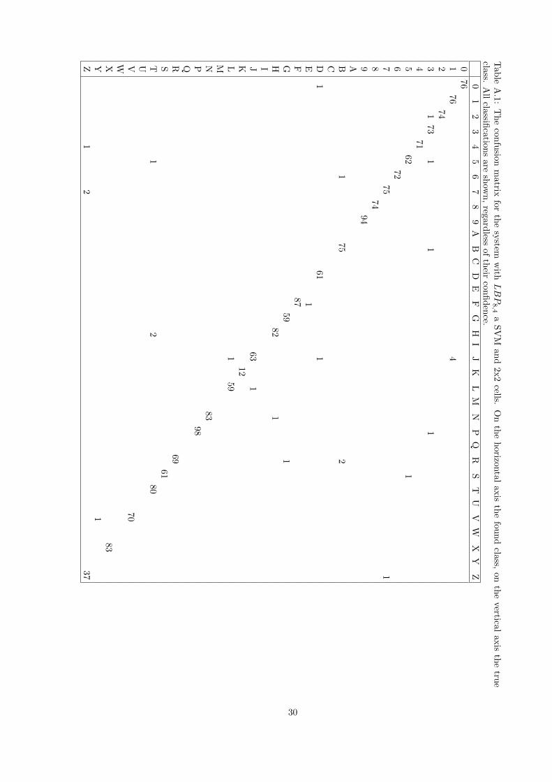
Based on the results, the decision is made to use LBP8,4, with a SVM and 2x2 cells. Itsaccuracy is slightly lower, but the speed is higher. Now it is now possible to create a confusionmatrix, showing the characters that have been classified versus the actual characters. Thisconfusion matrix is shown in appendix A.

The characters that are not classified correct are shown in appendix B. For comparison, thefaulty classifications are shown for LBP8,6 with 2x2 cells as well.

Linear kernel The kernel used in the previous experiments is the Radial Basis Function. In somecases it is faster to use a linear kernel. This is tested with the chosen system. The accuracyachieved with the linear kernel is 98.2% compared to 98.5% with the RBF kernel.

4.4 Speed

Since a fast recognition is a goal of this research, the required time to classify a character ismeasured.

16

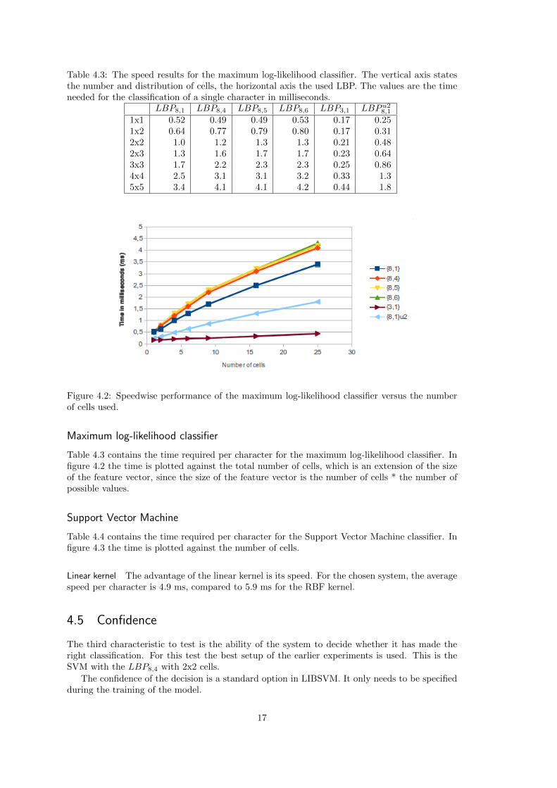
Table 4.3: The speed results for the maximum log-likelihood classifier. The vertical axis statesthe number and distribution of cells, the horizontal axis the used LBP. The values are the timeneeded for the classification of a single character in milliseconds.

LBP8,1 LBP8,4 LBP8,5 LBP8,6 LBP3,1 LBPu28,1

1x1 0.52 0.49 0.49 0.53 0.17 0.251x2 0.64 0.77 0.79 0.80 0.17 0.312x2 1.0 1.2 1.3 1.3 0.21 0.482x3 1.3 1.6 1.7 1.7 0.23 0.643x3 1.7 2.2 2.3 2.3 0.25 0.864x4 2.5 3.1 3.1 3.2 0.33 1.35x5 3.4 4.1 4.1 4.2 0.44 1.8

Figure 4.2: Speedwise performance of the maximum log-likelihood classifier versus the numberof cells used.

Maximum log-likelihood classifier

Table 4.3 contains the time required per character for the maximum log-likelihood classifier. Infigure 4.2 the time is plotted against the total number of cells, which is an extension of the sizeof the feature vector, since the size of the feature vector is the number of cells * the number ofpossible values.

Support Vector Machine

Table 4.4 contains the time required per character for the Support Vector Machine classifier. Infigure 4.3 the time is plotted against the number of cells.

Linear kernel The advantage of the linear kernel is its speed. For the chosen system, the averagespeed per character is 4.9 ms, compared to 5.9 ms for the RBF kernel.

4.5 Confidence

The third characteristic to test is the ability of the system to decide whether it has made theright classification. For this test the best setup of the earlier experiments is used. This is theSVM with the LBP8,4 with 2x2 cells.

The confidence of the decision is a standard option in LIBSVM. It only needs to be specifiedduring the training of the model.

17

Table 4.4: The speed results for the Support Vector Machine classifier. The vertical axis statesthe number and distribution of cells, the horizontal axis the used LBP. The values are the timeneeded for the classification of a single character in milliseconds.

LBP8,1 LBP8,4 LBP8,5 LBP8,6 LBP3,1 LBPu28,1

1x1 2.6 2.1 2.0 1.9 0.70 1.91x2 4.9 3.3 3.2 3.1 0.55 2.32x2 8.8 5.6 5.3 5.2 0.65 4.62x3 13 8.7 7.7 7.4 0.68 6.33x3 19 13 11 11 0.85 9.24x4 35 25 22 20 1.2 155x5 57 42 37 34 1.7 24

Figure 4.3: Speedwise performance of the SVM versus the number of cells used.

18

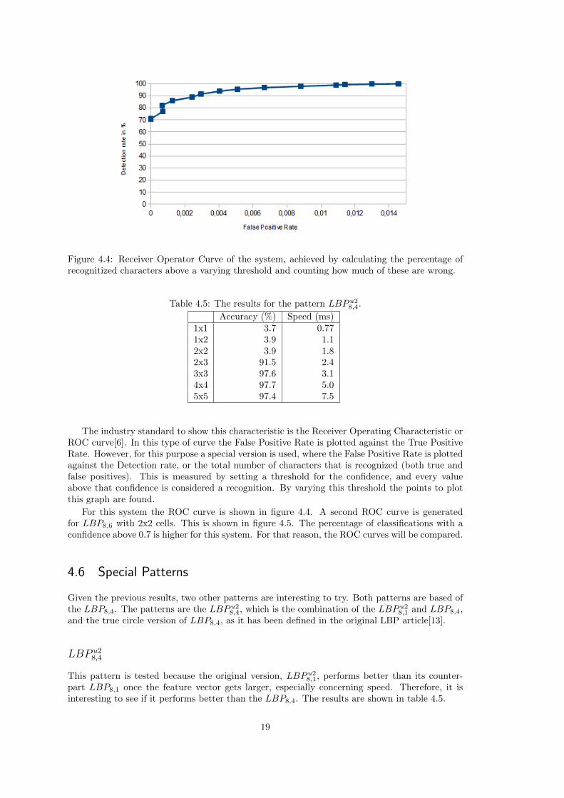
Figure 4.4: Receiver Operator Curve of the system, achieved by calculating the percentage ofrecognitized characters above a varying threshold and counting how much of these are wrong.

Table 4.5: The results for the pattern LBPu28,4.

Accuracy (%) Speed (ms)1x1 3.7 0.771x2 3.9 1.12x2 3.9 1.82x3 91.5 2.43x3 97.6 3.14x4 97.7 5.05x5 97.4 7.5

The industry standard to show this characteristic is the Receiver Operating Characteristic orROC curve[6]. In this type of curve the False Positive Rate is plotted against the True PositiveRate. However, for this purpose a special version is used, where the False Positive Rate is plottedagainst the Detection rate, or the total number of characters that is recognized (both true andfalse positives). This is measured by setting a threshold for the confidence, and every valueabove that confidence is considered a recognition. By varying this threshold the points to plotthis graph are found.

For this system the ROC curve is shown in figure 4.4. A second ROC curve is generatedfor LBP8,6 with 2x2 cells. This is shown in figure 4.5. The percentage of classifications with aconfidence above 0.7 is higher for this system. For that reason, the ROC curves will be compared.

4.6 Special Patterns

Given the previous results, two other patterns are interesting to try. Both patterns are based ofthe LBP8,4. The patterns are the LBPu2

8,4, which is the combination of the LBPu28,1 and LBP8,4,

and the true circle version of LBP8,4, as it has been defined in the original LBP article[13].

LBP u28,4

This pattern is tested because the original version, LBPu28,1, performs better than its counter-

part LBP8,1 once the feature vector gets larger, especially concerning speed. Therefore, it isinteresting to see if it performs better than the LBP8,4. The results are shown in table 4.5.

19

Figure 4.5: Receiver Operator Curve of LBP8,6 with 2x2 cells, achieved by calculating thepercentage of recognitized characters above a varying threshold and counting how much of theseare wrong.

Circular LBP8,4

This pattern is only tested to confirm that the simplification of the pattern to a square ispermitted. The original LBP theory specifies that the pattern should be circular. However, thatis to ensure rotational invariance, which is of no concern in this application and a simplificationwill therefore be faster.

This pattern is only tested against the best performer, LBP8,4 with 2x2 cells. The circularversion scores 97.5%.

20

CHAPTER 5

Conclusion

5.1 Accuracy

In the Python prototype system[15], an accuracy of 94.3% was achieved. The best accuracyachieved in the current research is 98.7%, which is considerably better than the earlier results.

The best system with regards to the speed results (which will be discussed later) achieves anaccuracy of 98.5%, so slightly less. This is achieved by the system using LBP8,4, a SVM and2x2 cells.

It should be noted that this score is per character. This means that for a license plate ofsix characters a score of 91.3% (0.9856 = 0.913) can be expected theoretically. However, thisis not true in an actual application, since an incorrectly classified character often is caused bydirt, a font that is not in the system or bad image quality. These factors will also apply to othercharacters on the license plate, which makes it more likely the other characters are classifiedwrong as well.

In addition, in ALPR systems syntactical analysis is performed. This can determine whethera character should be numerical or alphabetical. This can increase recognition rates for an entireplate in a way that is not possible for single characters.

Classifiers

The performance of the maximum log-likelihood classifier is less than the performance of theSupport Vector Machine. This is according to expectations, since the Support Vector Machinedoes not assume statistically independent histogram counts. The best accuracy scored withthe Maximum log-likelihood classifier is 85.1%. Although the maximum log-likelihood classifieris indeed faster than the SVM, the much higher accuracy of the SVM makes it the preferredclassifier in all cases.

For the kernel in the SVM, the choice can be made to use the linear kernel instead of theRBF. The accuracy is slightly less, at 98.1% instead of 98.5%, but there is a time advantage andit might be interesting for further research.

Patterns

The best performing patterns are the LBP8,4/5/6 ones. This has been predicted theoreticallyprior to the experiments, as described in section 3.4.

Remarkable is the bad performance of LBP3,1 when only one or two cells are used. Looking atthe confusion matrix, all characters are placed in one class for these systems. This could possiblyindicate the number of features is simply too small to be able to identify the character. It is alsopossible that the pattern is too small to capture the spatial characteristics of the character.

Looking at the math, since only three points are used, there is a total of 23 = 8 possiblevalues. That means that when using only one cell, the feature vector consists of only eightelements. Using two cells this is increased to sixteen. These are very low-dimensional vectors,

21

especially considering the amount of data, about 1500 values, that is fed into them. This willcreate large values in the feature vector, which will not differ a lot.

This hypothesis is confirmed by the fact that with more cells the performance is actuallybetter and when using 5x5 cells can even be considered fairly good, scoring a recognition rate of95.1% with the SVM.

The accuracy of LBPu28,4 is tested as well, since LBPu2

8,1 performs better than LBP8,1. However,LBPu2

8,4’s accuracy is less than that of LBP8,4. This indicates that LBP8,4 is already reachingthe limits of the possibilities of this system, and might be the best suited for this problem.

Also tested is the circular version of LBP8,4. Its score is not as good as that of the simplified(square) LBP8,4. This shows that using the simplified version is not decreasing accuracy in thisapplication, while it does improve the speed-wise performance.

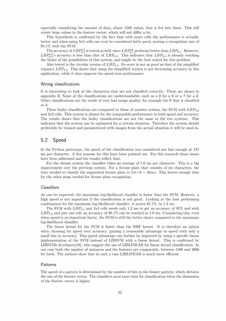
Wrong classifications

It is interesting to look at the characters that are not classified correctly. These are shown inappendix B. Some of the classifications are understandable, such as a D for a 0 or a 7 for a Z.Other classifications are the result of very bad image quality, for example the P that is classifiedas 3.

These faulty classifications are compared to those of another system, the SVM with LBP8,6

and 2x2 cells. This system is chosen for the comparable performance in both speed and accuracy.The results shows that the faulty classifications are not the same in the two systems. Thisindicates that the system can be optimized for a certain situation. Therefore the system shouldpreferably be trained and parametrized with images from the actual situation it will be used in.

5.2 Speed

In the Python prototype, the speed of the classification was considered not fast enough at 137ms per character. A few reasons for this have been pointed out. For this research those issueshave been addressed and the results reflect that.

For the chosen system the classifier takes an average of 5.6 ms per character. This is a bigimprovement over the previous system. For a license plate that consists of six characters, thetime needed to classify the segmented license plate is 5.6 ∗ 6 = 34ms. This leaves enough timefor the other steps needed for license plate recognition.

Classifiers

As can be expected, the maximum log-likelihood classifier is faster than the SVM. However, ahigh speed is not important if the classification is not good. Looking at the best performingcombination for the maximum log-likelihood classifier, it scores 85.1%, in 1.3 ms.

The SVM with LBP3,1 and 4x4 cells needs only 1.2 ms to get an accuracy of 95% and withLBP8,6 and just one cell, an accuracy of 98.1% can be reached in 1.9 ms. Considering this, evenwhen speed is an important factor, the SVM is still the better choice compared to the maximumlog-likelihood classifier.

The linear kernel for the SVM is faster than the RBF kernel. It is therefore an optionwhen choosing for speed over accuracy, gaining a reasonable advantage in speed with only asmall loss in accuracy. This speed advantage can further be improved by using a specific linearimplementation of the SVM instead of LIBSVM with a linear kernel. This is confirmed byLIBSVMs developers[16], who suggest the use of LIBLINEAR for linear kernel classification. Inour case both the number of instances and the features are comparable, between 1500 and 2000for both. The authors show that in such a case LIBLINEAR is much more efficient.

Patterns

The speed of a pattern is determined by the number of bits in the binary pattern, which dictatesthe size of the feature vector. The classifiers need more time for classification when the dimensionof the feature vector is higher.

22

Future research can be conducted to why the SVM needs more time to classify the smallerpatterns like LBP8,4 than the wider patterns such as LBP8,6.

5.3 Confidence

As figure 4.4 shows, the confidence of the classifications does not have the performance we hopedfor. When the requirement is that the classification correctness is guaranteed, only between 70and 75% is recognized. On the other hand, when all the possible classifications have to be made,1.5% of the classifications is false.

This second statement is the same as stating the accuracy is 98.5%. The problem is thatthere is no way of determining whether the given classification is correct. This is a problem,since a classifier that knows when the classification is correct is required in a lot of situations.For instance, in law enforcement it is vital that for example speeding tickets are not delivered tothe wrong person.

In other situations it might be less important. In situations with a database of allowed plates,such as a parking system with a ‘whitelist’ containing license plates that are allowed into theparking lot. Here a faulty classification will often only result in not opening the gates, andsecondary systems can take over.

As a single value for the confidence per system, the percentage of correct characters with aconfidence above 0.7 is used. For the used system, this percentage is 78.1%. Other combinationsperform better, meaning they are more suited for a system where confidence is important. Forexample, LBP8,6 with 2x2 cells has 81.5% correct classifications with a confidence above 0.7.

To make a better comparison, the ROC curve is generated for LBP8,6. This is shown in figure4.5. Like in the previous paragraph, the ROC curve shows that this system is more confident. Itcrosses 90% detection rate at a false positive rate of 0.0012, compared to around 0.0025 for thesystem using LBP8,4. This shows that the choice for a system should be made based on threecharacteristics: the accuracy, the speed and the confidence.

It should be noted that the measure for confidence used here is the probability given by theSVM. This probability indicates how likely the character is of a certain class. It is not completelyclear what method LIBSVM uses to calculate these probabilities. For further research, improvingthe confidence by investigating this method can be considered.

Other methods to increase confidence include the use of the difference in probabilities betweenthe best and the second best classes. Another possibility is to create a system that certain ofthe answer when the probability is higher than a certain threshold. If the confidence is lowerthan this threshold it is decreasingly confident. Increasing the confidence by such methods is asuggestion for further research.

5.4 Usability in real-life systems

As stated in the previous section, the inability of determining whether the classification is correctwhen a high recognition rate is required, might somewhat limit the possibilities for this method.However, there are several applications considerable.

The first is the system already described, with a whitelist of allowed plates. If a plate is notin the system different systems can be used. For example a second try with a new image, a moreadvanced but slower method or maybe even a human operator can take over.

The second is that the system can be used with a higher threshold for the confidence, guar-anteeing a correct classification. This is at the cost of a lower recognition rate. If the plate isnot recognized by the system, a secondary system can be used, similarly to the earlier situation.

In both situations the plus of this system is its high speed, classifying the character veryfast and reasonably accurate. If it recognizes the character in this case, it is a speed advantage.Otherwise, it is only a minor penalty. In both methods, the chance of a good classification isstill higher than that of a wrong one. This makes the choice for this classifier as a pre-classifierjustifiable.

23

Figure 5.1: Over-segmentation of the word ‘darn’ as given in [14].

Figure 5.2: Graph showing the possible paths in the over-segmented word ‘darn’, with the boundbetween the segments being the nodes. Taken from [14].

5.5 Future work

The high speed of the proposed system allows for a new type of license plate segmentation. Thismethod is based on the confidence of the classifier.

The idea is to have an over-segmentation in which the license plate is segmented in moresegments than there are characters. By classifying combinations of neighbouring segments anddetermining the confidences these groups have, a path that describes which segments to combinecan be determined.

The idea is based on a presentation given by Shafait[14]. The method described is designedfor normal text segmentation, but it could work for license plate segmentation as well. Themethod is best shown using the images used in the presentation. The over-segmentation is givenin figure 5.1. By combining some of these segments, several paths through the word can befound, using the segments as nodes, as shown in figure 5.2. Choosing the correct path is doneby assigning a cost to each edge, and using a dynamic programming algorithm to determine theleast cost. This is shown in 5.3.

The only difference between the proposed system and the system given by Shafait is thatthe confidence is a ‘positive’ measure instead of a cost, so not the minimum but the maximumshould be found.

24

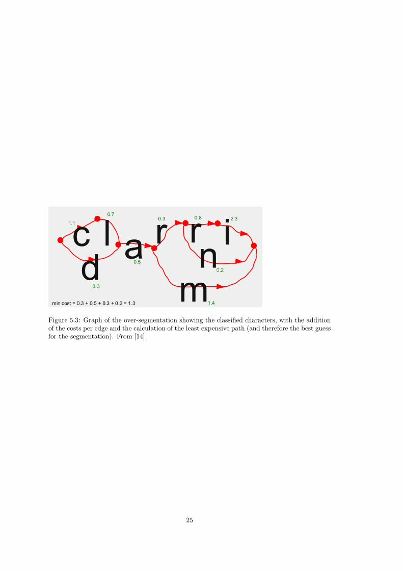
Figure 5.3: Graph of the over-segmentation showing the classified characters, with the additionof the costs per edge and the calculation of the least expensive path (and therefore the best guessfor the segmentation). From [14].

25

26

Bibliography

[1] How license plate recognition works. http://www.licenseplatesrecognition.com/

how-lpr-works.html.

[2] Parkingware bv. http://www.parkingware.com.

[3] Chih-Chung Chang and Chih-Jen Lin. LIBSVM: A library for support vector machines.ACM Transactions on Intelligent Systems and Technology, 2:27:1–27:27, 2011. Softwareavailable at http://www.csie.ntu.edu.tw/~cjlin/libsvm.

[4] Corinna Cortes and Vladimir Vapnik. Support-vector networks. In Machine Learning, pages273–297, 1995.

[5] Navneet Dalal and Bill Triggs. Histograms of oriented gradients for human detection. In InCVPR, pages 886–893, 2005.

[6] Tom Fawcett. Roc graphs: Notes and practical considerations for researchers. Technicalreport, HP Laboratories, 2004.

[7] V. Koval, V. Turchenko, V. Kochan, A. Sachenko, and G. Markowsky. Smart license platerecognition system based on image processing using neural network. In In Proceedings ofthe Second IEEE International Workshop on Advanced Computing Systems: Technology andApplications, 2003, pages 123–127, 2003.

[8] Halina Kwasnicka and Bartosz Wawrzyniak. License plate localization and recognition incamera pictures. In AI-METH 2002 - Artificial Intelligence Methods, 2002.

[9] Anish Lazrus and Siddhartha Choubey. A robust method of license plate recognition using.In International Journal of Computer Science and Information Technologies, Vol. 2 (4),pages 1494–1497, 2011.

[10] Xin Li. Vehicle license plate detection and recognition. Master’s thesis, University of Mis-souri, 2010.

[11] L. Liu, H. Zhang, A. Feng, X. Wan, and J. Guo. Simplified local binary pattern descrip-tor for character recognition of vehicle license plate. In Computer Graphics, Imaging andVisualization (CGIV), 2010 Seventh International Conference on, pages 157–161. IEEE,2010.

[12] Ondrej Martinsky. Algorithmic and mathemetical principles of automatic number platerecognition systems. Bachelor’s thesis, Brno University of Technology, 2007.

[13] Timo Ojala, Matti Pietikainen, and Topi Maenpaa. Gray scale and rotation invariant textureclassification with local binary patterns. In PROCEEDINGS OF THE SIXTH EUROPEANCONFERENCE ON COMPUTER VISION (ECCV2000), pages 404–420, 2000.

[14] Dr.-Ing. Faisal Shafait. Document image analysis with ocropus. In IEEE InternationalMultitopic Conference, 2009.

27

[15] Gijs van der Voort, Fabien Tesselaar, Taddeus Kroes, Richard Torenvliet, and Jayke Meijer.Using local binary patterns to read license plates in photographs. Labreport ComputerVision course at the University of Amsterdam, 2011.

[16] Chih wei Hsu, Chih chung Chang, and Chih jen Lin. A practical guide to support vector clas-sification. Technical report, Department of Computer Science, National Taiwan University,2010.

28

APPENDIX A

Confusion Matrix

29

Tab

leA

.1:

Th

eco

nfu

sionm

atrix

for

the

system

with

LBP8,4

aS

VM

an

d2x2

cells.O

nth

eh

orizo

ntal

axis

the

foun

dclass,

onth

evertical

axis

the

true

class.

All

classifica

tions

aresh

own

,reg

ardless

of

their

con

fid

ence.

01

23

45

67

89

AB

CD

EF

GH

IJ

KL

MN

PQ

RS

TU

VW

XY

Z0

76

176

42

743

173

11

14

71

562

16

727

751

874

994

AB1

75

2CD

161

1E

1F

87

G59

1H

82

1IJ

63

1K

12

L1

59

MN83

P98

QR69

S61

T1

280

UV70

WX83

Y1

Z1

237

30

APPENDIX B

Misclassified characters

Figure B.1: Characters that are classified incorrect by the system using a SVM, LBP8,4 and 2x2cells. The class that is found is shown above the image.

31

Figure B.2: Characters that are classified incorrect by the system using a SVM, LBP8,6 and 2x2cells. The class that is found is shown above the image.

32

APPENDIX C

LIBSVM with C++

The usage of LIBSVM with C++ is not well documented. Here, an explanation will be given toconvert a dataset consisting of vectors of some kind to a svm problem which can be used by thefunctions provided by the file svm.c through svm.h.

svm problem

A svm problem is a struct in svm.h. This describes the entire problem, and as such is passed tothe function svm train to create a svm model datatype. The svm problem struct contains thefollowing data:

• int l The number of vectors in the problem.

• double* y The class indentifier of each of the vectors in the problem.

• svm node** x The LIBSVM representation of the vectors.

svm node

A svm node is a single node in the vector representation. It has the following parameters:

• int index The index of this value in the vector.

• double value The value.

Creating a SVM problem from a set of vectors

For the creation of the SVM problem, each vector needs to be transformed into an array ofsvm node’s. At the end of this vector a node with index −1 has to be appended. This is toidentify the end of the array. The reason that is necessary is that LIBSVM uses what is calleda sparse dataformat, in which each vector element with value 0 can be omitted (hence the needfor indices).

All these arrays of svm nodes than have to be added as elements of a new array, creating a2D array, which can then be used as x in the svm problem. For each of these arrays of svm node’srepresenting a vector, the class has to be added to an other array, in the same order, which isthe array of doubles y in the svm problem.

33

Classification

In order to classify a vector, it has to be converted into an array of svm nodes’s the same way asearlier, with a node with index -1 at the end. The svm model and this array can then be passedto functions like svm predict, which returns the predicted class of this example.

34