Harmonic Flow for Histogram Matching

Thomas Batard and Marcelo Bertalmıo

Department of Information and Communication TechnologiesUniversity Pompeu Fabra, Barcelona, Spain

thomas.batard,marcelo.bertalmio@upf.edu

Abstract. We present a method to perform histogram matching be-tween two color images based on the concept of harmonic mapping be-tween Riemannian manifolds. The key idea is to associate the histogramof a color image to a Riemannian manifold. In this context, the energy ofthe matching between the two images is measured by the Dirichlet energyof the mapping between the Riemannian manifolds. Then, we assimilateoptimal matchings to critical points of the Dirichlet energy. Such pointsare called harmonic maps. As there is no explicit expression for harmonicmaps in general, we use a gradient descent flow with boundary conditionto reach them, that we call harmonic flow. We present an application tocolor transfer, however many others applications can be envisaged usingthis general framework.

Keywords: Histogram matching, Variational method, Riemannian ge-ometry, Dirichlet energy, Color transfer.

1 Introduction

As mentioned by Ling and Okada [14], histogram-based local descriptors are usedin many computer vision tasks, such as shape matching, image retrieval, textureanalysis, color analysis, 3D object recognition. See also [14] for references. Inorder to compare histograms, it is necessary to match them first in many casesbecause they are not aligned (due to shape deformation, lighting conditionschange, noise, etc). In [14], they make use of the Earth Moving’s Distance (EMD)to compare histograms, a method that involves a histogram matching step.

In this paper, we provide a new distance for comparing histograms based onthe Dirichlet energy. As the EMD, it is based on optimal matching between twosets. We present a straightforward application of histogram matching to colortransfer. However, we would like to point out that this general framework can beapplied to the computer vision tasks mentioned above up to small adjustments.

1.1 Color Transfer

In cinema post-production and professional photography, it is sometimes re-quired to adjust the colors of a rendered image with respect to the colors of an

This work was supported by European Research Council, Starting Grant ref. 306337.The second author acknowledges partial support by Spanish grants AACC, ref.TIN2011-15954-E, and Plan Nacional, ref. TIN2012-38112.

F. Huang and A. Sugimoto (Eds.): PSIVT 2013 Workshops, LNCS 8334, pp. 145–156, 2014.c© Springer-Verlag Berlin Heidelberg 2014

146 T. Batard and M. Bertalmıo

other image. Such a technique is called color transfer. In the color transferliterature, the rendered image is usually called source image, and the other oneis called reference image. Color transfer methods can be used for pure artisticpurpose, or to solve technical issues. There exist plenty of techniques to per-form color transfer between two images, but they all follow the same generalidea: produce an image that shares the details of the source image and the colorpalette of the reference image. We can distinguish three classes of color transfermethods.

Global Approaches. The global approaches only take into account the whole his-togram information of the two images, i.e. global information, to perform thetransfer of colors. As a consequence, these approaches modify the pixels of thesource image of same colors in the same way, regardless of their location in theimage and the values of the neighboring pixels.

The seminal work of Reinhard et al. [21] for color transfer is based on statis-tical matching: the color histograms of the two images are first expressed in anuncorrelated space lαβ, then the histogram of the source image is modified insuch a way that the mean and variance along each one of the three axis matchwith the one of the reference image. A similar approach has been adopted byKotera [13] where the statistical correspondence is done through the PrincipalComponent Analysis of the color histograms expressed in the RGB space. Letus also mention the approach of Pitie et al. [18] who make use of probability dis-tributions transfer in color spaces for performing color transfer between images.

Because these methods are global, the details of the source image as well asthe color distribution of the reference image might not be preserved correctly.

Local and Mixed Approaches. The local approaches take into account the loca-tion of the colors in the images and the values of the neighboring pixels, but notthe global information. Local approaches are mainly used when the two imagesshare some content (see e.g. [3],[4],[11]).

The mixed approaches both take into account global, i.e. histogram, infor-mation as well as local information to perform color transfer. They includemost of the variational formulations of the color transfer literature (see e.g.[5],[9],[17],[19],[20],[25]).

In this paper, we are interested in the general case, i.e. the two images are notrequired to share any content. The global and mixed approaches aforementionedapply to any images, unlike the local approaches. Even if the mixed approachesprovide better results than global approaches in general, it is still possible tofind examples where the methods fail, due the creation of artefacts, a lack ofpreservation of scene details and/or color palette, an unnatural look, etc.

Hence, we claim that there is still room for improvment in color transfer.

1.2 Our Contribution

In this paper, we present a new formulation for histogram matching betweentwo images (or patches) as the problem of finding an equilibrium state for the

Harmonic Flow for Histogram Matching 147

energy of the mapping of the color histogram of the source image onto the oneof the reference image. More precisely, we make use of the theory of harmonicmapping between Riemannian manifolds.

Harmonic maps are critical points of the Dirichlet energy, and generalize theconcepts of geodesic curves and minimal surfaces. Harmonic mapping betweenRiemannian manifolds has been studied for a while (see [8] and the referencestherein). Whereas there exists no general theory providing an expression of har-monic maps, the problem of the existence of harmonic maps has been widelyinvestigated and different approaches have been adopted. In this paper, we fol-low the approach of deformation by heat flow of Eells and Sampson [7], that wecall harmonic flow. The harmonic flow is nothing but the continuous formula-tion of the gradient descent associated to the Dirichlet energy. In particular theyshowed that, under some assumption on the curvature of the target manifold,the heat flow converges to a harmonic map.

The Dirichlet energy and its minimization problem were introduced for imageprocessing by Sochen et al. [22] with an application to color image denoising.Apart from image processing, they have been applied (in a simplified form) forcomputer vision tasks like optimal flow estimation [2] and shape analysis [1]. Inour approach of histogram matching from harmonic mapping, the Riemannianmanifolds considered are related to the histograms of the images, and the localvariations of the histograms are encoded into the Riemannian metrics. The choiceof the Riemannian manifolds involved in our variational formulation makes theproposed color transfer method be a global approach. However, we would like topoint out that others choices of Riemannian manifolds would lead to mixed orlocal approaches.

2 Harmonic Flow between Riemannian Manifolds

2.1 Harmonic Mapping between Riemannian Manifolds

Let (M, g) and (N, h) be two smooth Riemannian manifolds. The Dirichlet en-ergy E of a map Φ : (M, g) −→ (N, h) is defined by

E(Φ) : =

∫M

|dΦ|2g−1⊗h dM =

∫M

hαβ∂Φα

∂xi

∂Φβ

∂xjgij dM (1)

where dΦ is the differential of Φ. The notation | |g−1⊗h stands for the norm withrespect to the metric g−1 ⊗ h. See [8] for more details.

The critical points of the energy (1) are called harmonic maps. They arethe solutions of the system

τ(Φ) : = ΔgΦi + Γ i

jk ∂μΦj∂νΦ

kgμν = 0, i = 1, · · · , dimN (2)

where Δg stands for the Laplace-Beltrami operator on (M, g) and Γ ijk are the

symbols of the Levi-Civita connection on (N, h).

148 T. Batard and M. Bertalmıo

The term τ(Φ) is called the tension field of the map Φ. There exists amore compact formulation for τ(Φ):

τ(Φ) = div(dΦ)

where div is the adjoint operator of the Levi-Civita covariant derivative ∇ onthe vector bundle Φ−1TN over M , i.e. it satisfies

∫M

〈∇ϕ, ψ〉g−1⊗h dM =

∫M

〈ϕ, div ψ〉h dM (3)

∀ϕ ∈ Γ (Φ−1TN) and ψ ∈ Γ (T ∗M ⊗ Φ−1TN) with compact support.

Harmonic maps appear in well-known contexts:

- If dim M=1, then the Dirichlet energy measures the length of curves in theRiemannian manifold (N, h) and the harmonic maps are the geodesics of (N, h).

- If dim M=2 and N = R3, the Dirichlet energy measures the area of surfaces

embedded in R3. The harmonic maps are then the minimal surfaces.

2.2 On the Harmonic Flow

In a very complete report, Eells and Lemaire [8] mentioned that there is no gen-eral theory to construct solutions of the system (2), i.e. harmonic maps betweenRiemannian manifolds. However, the problem of the existence of non trivial so-lutions has been studied for a while and is still under investigation. The classicapproach is formulated as follows: ”Let Φ0 : M −→ N be a map of Riemannianmanifolds. Can Φ0 be deformed into a harmonic map Φ : M −→ N?” There aredifferent approaches to attack this problem:

- The direct method of variational theory (lower semicontinuity of the Dirichletenergy on compact subsets on the space C(M,N) of maps, in a suitable weaktopology). This technique works well for dim M = 1, 2 (see Morrey [15]), butnot for dim M ≥ 3 in general.- Deformation by heat flow: these are the approaches of Eells and Sampson [7],Hamilton [12], to show that the answer is ”yes” if the sectional curvature of Nis nonpositive.- Morse theory in manifolds of maps: that was used for instance by Palais [16]to prove the existence of geodesics joining two points.

In this paper, we focus on the technique of deformation by heat flow, thatwe call harmonic flow.

From now on, we assume that M and N are compact manifolds, and M hasa boundary ∂M . Let ψ : ∂M −→ N and Φ0 : M −→ N such that Φ0|∂M = ψ.

Harmonic Flow for Histogram Matching 149

We consider the harmonic flow with Dirichlet boundary conditions⎧⎪⎪⎪⎪⎨⎪⎪⎪⎪⎩

∂Φ/∂t = div(dΦ) on M × R+

Φ = Φ0 on M × 0

Φ = ψ on ∂M × R+

(4)

Then, there is a solution for the problem (4) defined for a short time [0, t1[.Moreover, E(Φ) is a strictly decreasing function of t, except at those values of tfor which τ(Φ) = 0.

We have the following theorem due to Hamilton.

Theorem 1. If the Riemannian sectional curvature of N is nonpositive then thesolution Φ of the system (4) is globally defined and converges towards a harmonicmap.

We refer to Hamilton [12] for more details about harmonic maps of manifoldswith boundary.

3 Harmonic Flow for (Color) Histogram Matching

3.1 From Color Image to Riemannian Manifold

Given an image I : Ω ⊂ R2 −→ RGB, the so-called tensor of structure of I is

the 2x2 matrix field ⎛⎝

∑3k=1(I

kx1)2

∑3k=1 I

kx1Ikx2

∑3k=1 I

kx1Ikx2

∑3k=1(I

kx2)2

⎞⎠ (5)

The eigenvalues and eigenvectors fields of (5) provide information about thelocal behaviour of the image. Indeed, the eigenvalues measure the highest andlowest directional variations of I and the corresponding eigenvectors give thedirections of these optimal variations. The tensor of structure has been widelyused for color image processing tasks (see e.g. [6] for segmentation, and [23],[24]for denoising/regularization purposes).

It turns out that the tensor of structure (5) is quite close to a Riemannianmetric. Indeed, if we denote by ψ the graph of the image I, i.e. the map

ψ : (x1, x2) −→ (x1, x2, I1(x1, x2), I

2(x1, x2), I3(x1, x2)),

then ψ determines the embedding of the manifold Ω into R5, and the Euclidean

metric on R5 induces a Riemannian metric g on Ω of the form

g =

⎛⎝1 +

∑3k=1(I

kx1)2

∑3k=1 I

kx1Ikx2

∑3k=1 I

kx1Ikx2

1 +∑3

k=1(Ikx2)2

⎞⎠ (6)

150 T. Batard and M. Bertalmıo

in the frame (∂/∂x1, ∂/∂x2). The couple (Ω, g) forms a compact Riemannianmanifold of dimension 2.

In [22], an anisotropic diffusion based on the Laplace-Beltrami operator Δg

associated to the metric (6) is performed for color image denoising/regularizationpurposes.

In the following paragraph, we extend this construction to manifolds of di-mension 3 in order to encode the local behavior of color images histograms intoRiemannian metrics.

3.2 Extension to Color Histogram

Let I : Ω ⊂ R2 −→ RGB be a color image. We denote by HI the function that

maps any color (r, g, b) to the number of pixels of color (r, g, b) in I. Let ψ bethe graph of the function βHI , β ≥ 0, i.e.

ψ : (r, g, b) −→ (r, g, b, βHI(r, g, b))

The map ψ determines the embedding of the compact manifold RGB of di-mension 3 into RGB × R. Then the Euclidean metric on RGB × R induces aRiemannian metric hβ on RGB of the form

hβ =

⎛⎜⎜⎜⎜⎜⎜⎝

1 + β2(∂ HI

∂ r

)2β2 ∂ HI

∂ r∂ HI

∂ g β2 ∂ HI

∂ r∂ HI

∂ b

β2 ∂ HI

∂ r∂ HI

∂ g 1 + β2(

∂ HI

∂ g

)2

β2 ∂ HI

∂ g∂ HI

∂ b

β2 ∂ HI

∂ r∂ HI

∂ b β2 ∂ HI

∂ g∂ HI

∂ b 1 + β2(∂ HI

∂ b

)2

⎞⎟⎟⎟⎟⎟⎟⎠

(7)

in the frame (∂/∂r, ∂/∂g, ∂/∂b). The couple (RGB, hβ) forms a compact Rie-mannian manifold of dimension 3.

Remark 1. Notice that such a construction can be done for images with anynumber of channels.

Assuming that the manifolds (M, g) and (N, h) are respectively of the form(RGB, hβ1) and (RGB, hβ2), we deduce that the harmonic flow (4) convergestowards a harmonic map if the sectional curvature of the Riemannian manifold(RGB, hβ2) is nonpositive. Let us distinguish two cases:

1. The case β2 = 0.The Riemannian metric hβ2 is then Euclidean (see formula (7)), the sectionalcurvature of (RGB, hβ2) is zero, and theorem 1 applies. In this case we obtainthe heat flow of the Laplace-Beltrami operator Δhβ1

since the terms Γ kij in the

tension field (2) vanish.

2. The case β2 > 0.In this case, we do not know if (RGB, hβ2) has a nonpositive sectional curvature

Harmonic Flow for Histogram Matching 151

or not. However, we do have a necessary condition for the sectional curvatureto be nonpositive. Indeed, it is mentioned in [10] that Riemannian manifoldsthat are hypersurfaces of Rn, n ≥ 4, can not have strictly negative sectional cur-vature. Hence, because the manifolds (RGB, hβ2) are hypersurfaces of R4 (seeconstruction in Sect. 2.2), we deduce that a necessary condition is that the sec-tional curvature of (RGB, hβ2) vanishes at least once. If not, then the theorem1 does not apply.

3.3 Implementation

We adopt a gradient descent approach to approximate the harmonic flow (4) forcolor histogram matching. The algorithm we propose is the following

⎧⎪⎪⎪⎪⎨⎪⎪⎪⎪⎩

Φt+dt = Φt − dt div(dΦt) on RGB × R+

Φ|t=0 = Φ0 on RGB × 0

Φt = Φ0|∂RGB on ∂RGB × R+

(8)

We stop the algorithm (8) at t = T when the Dirichlet energy E(Φt) stopsdecreasing. We would like to remind that we do not have guarantee that thesystem (8) is globally defined if the sectional curvature of (RGB, hβ2) is notnonpositive. Hence, the map ΦT might not be harmonic.

The main task is to compute a discrete approximation of the operator div. Toperform this, our approach is based on a generalization of the Euclidean case.The classic approach to compute a discrete approximation of the Euclidean diver-gence div : Γ (T ∗Ω) −→ C∞(Ω) is to make use of its adjoint operator property.Indeed, by definition, we have the equality

∫Ω

div η ϕ dΩ =

∫Ω

〈η, dϕ 〉 dΩ (9)

for ϕ ∈ C∞(Ω) and η ∈ Γ (T ∗Ω) with compact support. Then, using for-ward differences for discretizing dϕ implies that div η must be discretized usingbackward differences. We extend this approach to the operator div : Γ (T ∗M ⊗Φ−1TN) −→ Γ (Φ−1TN) using the discrete version of the formula (3). The ex-plicit expression of the discrete divergence operator is given in the Appendix.

4 An Application of Histogram Matching to ColorTransfer

4.1 From Harmonic Mapping between Color Histograms to ColorTransfer

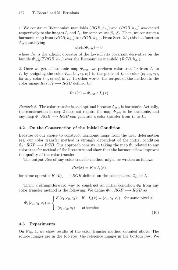
The method we propose for performing color transfer from a reference image Irto a source image Is is composed of two steps.

152 T. Batard and M. Bertalmıo

1. We construct Riemannian manifolds (RGB, hβs) and (RGB, hβr ) associatedrespectively to the images Is and Ir , for some values βs, βr. Then, we construct aharmonic map from (RGB, hβs) to (RGB, hβr). From Sect. 2.1, this is a functionΦcrit satisfying

div(dΦcrit) = 0

where div is the adjoint operator of the Levi-Civita covariant derivative on thebundle Φ−1

crit(TRGB, hβr) over the Riemannian manifold (RGB, hβs).

2. Once we get a harmonic map Φcrit, we perform color transfer from Ir toIs by assigning the color Φcrit(c1, c2, c3) to the pixels of Is of color (c1, c2, c3),for any color (c1, c2, c3) in Is. In other words, the output of the method is thecolor image Res : Ω −→ RGB defined by

Res(x) = Φcrit Is(x)

Remark 2. The color transfer is said optimal because Φcrit is harmonic. Actually,the construction in step 2 does not require the map Φcrit to be harmonic, andany map Φ : RGB −→ RGB can generate a color transfer from Ir to Is.

4.2 On the Construction of the Initial Condition

Because of our choice to construct harmonic maps from the heat deformation(4), our color transfer method is strongly dependent of the initial conditionΦ0 : RGB −→ RGB. Our approach consists in taking the map Φ0 related to anycolor transfer method of the literature and show that the harmonic flow improvesthe quality of the color transfer.

The output Res of any color transfer method might be written as follows

Res(x) = K Is(x)for some operator K : CIs −→ RGB defined on the color palette CIs of Is.

Then, a straightforward way to construct an initial condition Φ0 from anycolor transfer method is the following. We define Φ0 : RGB −→ RGB as

Φ0(c1, c2, c3) =

⎧⎨⎩

K(c1, c2, c3) if Is(x) = (c1, c2, c3) for some pixel x

(c1, c2, c3) otherwise(10)

4.3 Experiments

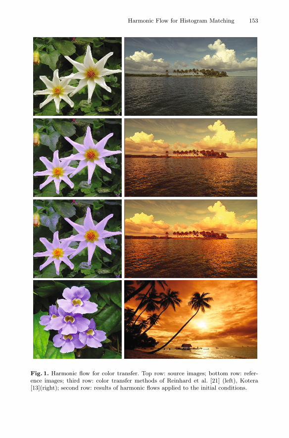
On Fig. 1, we show results of the color transfer method detailed above. Thesource images are in the top row, the reference images in the bottom row. We

Harmonic Flow for Histogram Matching 153

Fig. 1. Harmonic flow for color transfer. Top row: source images; bottom row: refer-ence images; third row: color transfer methods of Reinhard et al. [21] (left), Kotera[13](right); second row: results of harmonic flows applied to the initial conditions.

154 T. Batard and M. Bertalmıo

apply the harmonic flow described above, for some parameters βs, βr, dt, on theimages of third row, and the results are shown in the second column.

More precisely, the initial conditions Φ0 are constructed following the method(10) applied to the algorithm of Reinhard et al. [21] (left column) and Kotera[13] (right column). The parameters of our algorithm are: βs = 0, βr = 0.07,dt = 0.001 (left), and βs = 0, βr = 0.001 , dt = 0.001 (right) . In both cases,we stopped the algorithm (8) at t = T when the Dirichlet energy E(Φt) stoppeddecreasing. As βr > 0 in these experiments, we do not have the guarantee thatΦT is a harmonic map.

We see that our results are coherent with what we expect from a color transfermethod: the output image provides fidelity with respect to both scene details ofthe source image and colors of the reference image. We observe that our methodmakes the color transfers be more realistic than the initial conditions. Indeed,under a right choice for the parameters of the ’flowers’ images color transfer,we can see that our method removes almost completely the violet that appearson the leaves in the initial condition. However, as the color transfer methodpresented here is global, the violet reduces on the flowers too. Regarding the’landscapes’ images color transfers, we see that the initial condition tends tomake the details in the clouds of the source image disappear. Applying theharmonic flow under a right choice for the parameters, allows us to recover apart of these details.

5 Conclusion

We have presented a new method for (color) histogram matching between twoimages, dealing with the Dirichlet energy of the mapping between Riemannianmanifolds. In this context, we relate histograms of images with Riemannianmanifolds, the local variations of the histograms being encoded by Riemannianmetrics. We have adopted a deformation by heat flow, that we called harmonicflow, in order to construct harmonic maps. As this stage, we are not able toguarantee that the harmonic flow converges in any case toward a harmonic map.Further work will then be devoted to establish more theoretical results about theheat flow approach as well as investigate other approaches to construct harmonicmaps.

We have presented an application to color transfer. The manifolds consideredin this paper only encode histogram information of images, i.e. global informa-tion, meaning that color transfers modify pixels of same color in the same way,without taking into account their location or the values of the neighboring pix-els. The examples presented have revealed the limits of such a global approach.However, the general framework introduced in this paper allows us to constructmixed and local approaches for color transfer by the construction of Riemannianmanifolds that take into account local information of images. This is the subjectof current research.

Finally, applications to computer vision can be envisaged from the construc-tion of histogram-based local descriptors based on the Dirichlet energy and har-monic mapping.

Harmonic Flow for Histogram Matching 155

References

1. Aflalo, Y., Kimmel, R., Zibulevsky, M.: Conformal Mapping with as Uniform asPossible Conformal Factor. SIAM J. of Imaging Sciences 6(1), 78–101 (2013)

2. Ben-Ari, R., Sochen, N.: A Geometric Framework and a New Criterion in OpticalFlow Modeling. J. Mathematical Imaging and Vision 33(2), 178–194 (2009)

3. Bertalmıo, M., Levine, S.: Variational Approach for the Fusion of Exposure Brack-eted Pairs. IEEE Trans. Image Processing 22(2), 712–723 (2013)

4. Bertalmıo, M., Levine, S.: Color Matching for Stereoscopic Cinema. Proc. of MI-RAGE 2013 6 (2013)

5. Delon, J.: Midway Image Equalization. J. Mathematical Imaging and Vision 21(2),119–134 (2004)

6. Di Zenzo, S.: A Note on the Gradient of a Multi-Image. Computer Vision, Graphicsand Image Processing 33(1), 116–125 (1986)

7. Eells, J., Sampson, J.H.: Harmonic Mappings of Riemannian Manifolds. AmericanJournal of Mathematics 86(1), 109–160 (1964)

8. Eells, J., Lemaire, L.: A Report on Harmonic Maps. Bull. London Math. Soc. 10,1–68 (1978)

9. Ferradans, S., Papadakis, N., Rabin, J., Peyre, G., Aujol, J.-F.: Regularized Dis-crete Optimal Transport. In: Kuijper, A., Bredies, K., Pock, T., Bischof, H. (eds.)SSVM 2013. LNCS, vol. 7893, pp. 428–439. Springer, Heidelberg (2013)

10. Gallot, S., Hulin, D., LaFontaine, J.: Riemannian Geometry. Springer (2004)

11. HaCohen, Y., Shechtman, E., Goldman, D.B., Lischinski, D.: Non-Rigid Dense Cor-respondence with Applications for Image Enhancement. ACM Trans. Graph. 30(4),Art. 70 (2011)

12. Hamilton, R.S.: Harmonic Maps of Manifolds with Boundary. Lecture in Mathe-matics, vol. 471. Springer (1975)

13. Kotera, H.: A Scene-Referred Color Transfer for Pleasant Imaging on Display. In:IEEE Int. Conf. Image Processing, vol. 2, pp. 5–8 (2012)

14. Ling, H., Okada, K.: An Efficient Earth Mover’s Distance Algorithm for Ro-bust Histogram Comparison. IEEE Trans. Pattern Analysis and Machine Intel-ligence 29(5), 840–853 (2007)

15. Morrey, C.B.: The Problem of Plateau on a Riemannian Manifold. Annals ofMathematics 49, 807–851 (1948)

16. Palais, R.S.: Morse Theory on Hilbert Manifolds. Topology 2, 299–340 (1963)

17. Papadakis, N., Provenzi, E., Caselles, V.: A Variational Model for Histogram Trans-fer of Color Images. IEEE Trans. Image Processing 20(6), 1682–1695 (2011)

18. Pitie, F., Kokaram, A., Dahyot, A.: Automated Color Grading using Colour Dis-tribution Transfer. Computer Vision and Image Understanding 107(1), 123–137(2007)

19. Pitie, F., Kokaram, A.: The Linear Monge-Kantorovitch Colour Mapping forExample-based Colour Transfer. In: Proc. IEEE Eur. Conf. Vis. Media Prod., pp.1–9 (2007)

20. Rabin, J., Peyre, G.: Wasserstein Regularization of Imaging Problem. In: Proc. of17th IEEE Int. Conf. Image Processing ICIP, pp. 1541–1544 (2011)

21. Reinhard, E., Ashikhmin, M., Gooch, B., Shirley, P.: Color Transfer between Im-ages. IEEE Computer Graphics and Applications 21(5), 34–41 (2001)

22. Sochen, N., Kimmel, R., Malladi, R.: A General Framework for Low Level Vision.IEEE Trans. Image Processing 7(3), 310–318 (1998)

156 T. Batard and M. Bertalmıo

23. Tschumperle, D., Deriche, R.: Vector-Valued Image Regularization with PDEs: ACommon Framework for Different Applications. IEEE Trans. Pattern Anal. Mach.Intell. 27(4), 506–517 (2005)

24. Weickert, J.: Anisotropic Diffusion in Image Processing. Teubner, Stuttgart (1998)25. Xiao, X., Ma, L.: Gradient-Preserving Color Transfer. Computer Graphics Fo-

rum 28(7), 1879–1886 (2009)

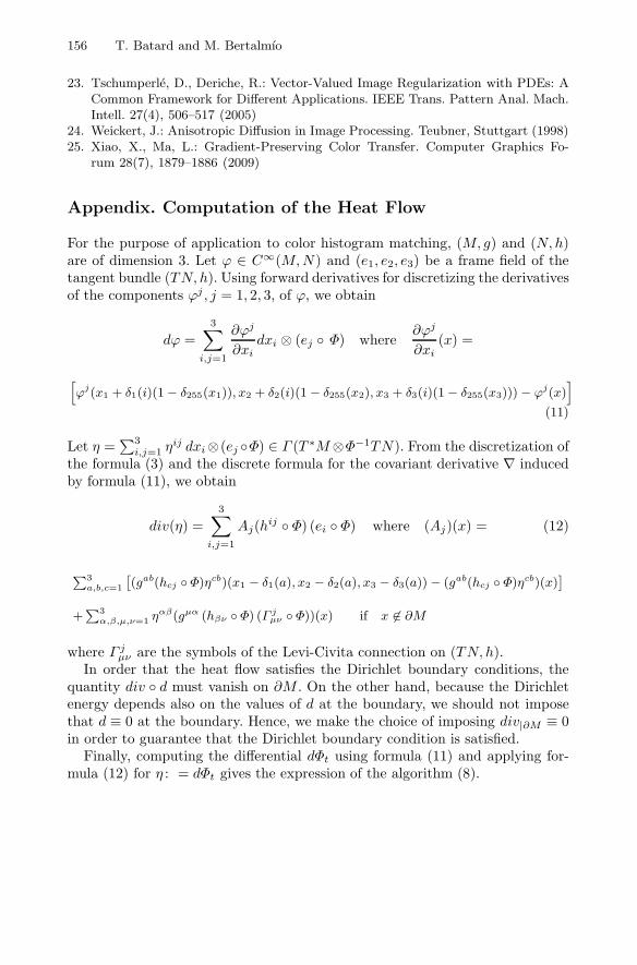
Appendix. Computation of the Heat Flow

For the purpose of application to color histogram matching, (M, g) and (N, h)are of dimension 3. Let ϕ ∈ C∞(M,N) and (e1, e2, e3) be a frame field of thetangent bundle (TN, h). Using forward derivatives for discretizing the derivativesof the components ϕj , j = 1, 2, 3, of ϕ, we obtain

dϕ =

3∑i,j=1

∂ϕj

∂xidxi ⊗ (ej Φ) where

∂ϕj

∂xi(x) =

[ϕj(x1 + δ1(i)(1− δ255(x1)), x2 + δ2(i)(1− δ255(x2), x3 + δ3(i)(1− δ255(x3)))− ϕj(x)

]

(11)

Let η =∑3

i,j=1 ηij dxi⊗(ej Φ) ∈ Γ (T ∗M⊗Φ−1TN). From the discretization of

the formula (3) and the discrete formula for the covariant derivative ∇ inducedby formula (11), we obtain

div(η) =

3∑i,j=1

Aj(hij Φ) (ei Φ) where (Aj)(x) = (12)

∑3a,b,c=1

[(gab(hcj Φ)ηcb)(x1 − δ1(a), x2 − δ2(a), x3 − δ3(a))− (gab(hcj Φ)ηcb)(x)

]

+∑3

α,β,μ,ν=1 ηαβ(gμα (hβν Φ) (Γ j

μν Φ))(x) if x ∈ ∂M

where Γ jμν are the symbols of the Levi-Civita connection on (TN, h).

In order that the heat flow satisfies the Dirichlet boundary conditions, thequantity div d must vanish on ∂M . On the other hand, because the Dirichletenergy depends also on the values of d at the boundary, we should not imposethat d ≡ 0 at the boundary. Hence, we make the choice of imposing div|∂M ≡ 0in order to guarantee that the Dirichlet boundary condition is satisfied.

Finally, computing the differential dΦt using formula (11) and applying for-mula (12) for η : = dΦt gives the expression of the algorithm (8).