Lecture # 3 Histogram Matching Spatial...

1

Digital Image Processing

Lecture # 3Histogram Matching

& Spatial Filtering

2

HISTOGRAM MATCHING (SPECIFICATION)

• HISTOGRAM EQUALIZATION DOES NOT ALLOWINTERACTIVE IMAGE ENHANCEMENT ANDGENERATES ONLY ONE RESULT: ANAPPROXIMATION TO A UNIFORM HISTOGRAM.

• SOMETIMES THOUGH, WE NEED TO BE ABLE TOSPECIFY PARTICULAR HISTOGRAM SHAPESCAPABLE OF HIGHLIGHTING CERTAIN GRAY-LEVELRANGES.

3

HISTOGRAM SPECIFICATION• THE PROCEDURE FOR HISTOGRAM-SPECIFICATION BASED

ENHANCEMENT IS:

– EQUALIZE THE LEVELS OF THE ORIGINAL IMAGE USING:

k

j

j

kn

nrTs

0

)(

n: total number of pixels,

nj: number of pixels with gray level rj,

L: number of discrete gray levels

4

HISTOGRAM SPECIFICATION

– SPECIFY THE DESIRED DENSITY FUNCTION AND OBTAIN THE

TRANSFORMATION FUNCTION G(z):

pz: specified desirable PDF for output

ki

k

i

zkk szpzGv 0

5


• THE NEW, PROCESSED VERSION OF THEORIGINAL IMAGE CONSISTS OF GRAYLEVELS CHARACTERIZED BY THE SPECIFIEDDENSITY pz(z).

)]([ )( 11 rTGzsGz In essence:

6

MAPPINGS

7


• OBTAIN THE HISTOGRAM OF THE GIVEN IMAGE

• MAP EACH LEVEL rK TO A LEVEL SK

• OBTAIN THE TRANSFORMATION FUNCTION G FROM THEGIVEN PZ (Z)

• PRECOMPUTE ZK FOR EACH VALUE OF SK

• FOR EACH PIXEL IN THE ORIGINAL IMAGE, IF THE VALUEOF THAT PIXEL IS rk MAP THIS VALUE TO ITSCORRESPONDING LEVEL SK, THEN MAP LEVEL SK INTO THEFINAL VALUE ZK

8


k nk pr(rk) sk pz(zk) vk nk

0 790 0.19 0.19 0 0 0

1 1023 0.25 0.44 0 0 0

2 850 0.21 0.65 0 0 0

3 656 0.16 0.81 0.15 0.15 790

4 329 0.08 0.89 0.2 0.35 1023

5 245 0.06 0.95 0.3 0.65 850

6 122 0.03 0.98 0.2 0.85 985

7 81 0.02 1.0 0.15 1.0 448

A 64X64 (4096 PIXELS) IMAGE WITH 8 GRAY LEVELS

9

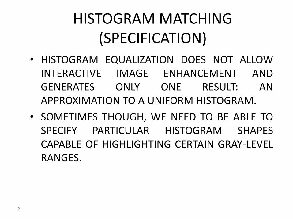
IMAGE ENHANCEMENT IN THE

SPATIAL DOMAIN

10


SPATIAL DOMAIN

12

GLOBAL/LOCAL HISTOGRAM EQUALIZATION

• IT MAY BE NECESSARY TO ENHANCE DETAILS OVER SMALL AREAS IN THEIMAGE

• THE NUMBER OF PIXELS IN THESE AREAS MAY HAVE NEGLIGIBLE INFLUENCEON THE COMPUTATION OF A GLOBAL TRANSFORMATION WHOSE SHAPEDOES NOT NECESSARILY GUARANTEE THE DESIRED LOCAL ENHANCEMENT

• DEVISE TRANSFORMATION FUNCTIONS BASED ON THE GRAY LEVELDISTRIBUTION IN THE NEIGHBORHOOD OF EVERY PIXEL IN THE IMAGE

• THE PROCEDURE IS:– DEFINE A SQUARE (OR RECTANGULAR) NEIGHBORHOOD AND MOVE THE

CENTER OF THIS AREA FROM PIXEL TO PIXEL.– AT EACH LOCATION, THE HISTOGRAM OF THE POINTS IN THE

NEIGHBORHOOD IS COMPUTED AND EITHER A HISTOGRAMEQUALIZATION OR HISTOGRAM SPECIFICATION TRANSFORMATIONFUNCTION IS OBTAINED.

– THIS FUNCTION IS FINALLY USED TO MAP THE GRAY LEVEL OF THE PIXELCENTERED IN THE NEIGHBORHOOD.

– THE CENTER IS THEN MOVED TO AN ADJACENT PIXEL LOCATION AND THEPROCEDURE IS REPEATED.

13

GLOBAL/LOCAL HISTOGRAM EQUALIZATION

14

USE OF HISTOGRAM STATISTICS FOR IMAGE ENHANCEMENT (Global)

• LET r REPRESENT A GRAY LEVEL IN THE IMAGE [0, L-1], AND LET p(ri )DENOTE THE NORMALIZED HISTOGRAM COMPONENTCORRESPONDING TO THE ith VALUE OF r.

• THE nth MOMENT OF r ABOUT ITS MEAN IS DEFINED AS

• WHERE m IS THE MEAN VALUE OF r (AVERAGE GRAY LEVEL)

i

nL

i

in rpmrr

1

0

iL

i i rprm

1

0

15

USE OF HISTOGRAM STATISTICS FOR IMAGE ENHANCEMENT (Global)

• THE SECOND MOMENT IS GIVEN BY

• WHICH IS THE VARIANCE OF r

• MEAN AS A MEASURE OF AVERAGE GRAY LEVEL IN THE IMAGE

• VARIANCE AS A MEASURE OF AVERAGE CONTRAST

i

L

i

i rpmrr

21

0

2

16

USE OF HISTOGRAM STATISTICS FOR IMAGE ENHANCEMENT (Local)

• LET (x,y) BE THE COORDINATES OF A PIXEL IN ANIMAGE, AND LET SX,Y DENOTE A NEIGBORHOOD OFSPECIFIED SIZE, CENTERED AT (x,y)

• THE MEAN VALUE mSXY OF THE PIXELS IN SX,Y IS

• THE GRAY LEVEL VARIANCE OF THE PIXELS INREGION SX,Y IS GIVEN BY

ts

Sts

tss rprmxy

xy ,

,

,

ts

Sts

stsS rpmrxy

xyxy ,

,

2

,

2

17

USE OF HISTOGRAM STATISTICS FOR IMAGE ENHANCEMENT

• THE GLOBAL MEAN AND VARIANCE ARE MEASUREDOVER AN ENTIRE IMAGE AND ARE USEFUL FORGROSS ADJUSTMENTS OF OVERALL INTENSITY ANDCONTRAST.

• A USE OF THESE MEASURES IN LOCALENHANCEMENT IS, WHERE THE LOCAL MEAN ANDVARIANCE ARE USED AS THE BASIS FOR MAKINGCHANGES THAT DEPEND ON IMAGECHARACTERISTICS IN A PREDEFINED REGION ABOUTEACH PIXEL IN THE IMAGE.

18

TUNGSTEN FILAMENT IMAGE

19

USE OF HISTOGRAM STATISTICS FOR IMAGE ENHANCEMENT

• A PIXEL AT POINT (x,y) IS CONSIDERED IF:– mSXY ≤ k0MG, where k0 is a positive constant less than 1.0, and MG is

global mean

– σsxy ≤ k2DG, where DG is the global standard deviation and k2 is apositive constant

– k1DG ≤ σsxy ,, with k1 < k2

• A PIXEL THAT MEETS ALL ABOVE CONDITIONS ISPROCESSED SIMPLY BY MULTIPLYING IT BY A SPECIFIEDCONSTANT, E, TO INCREASE OR DECREASE THE VALUE OFITS GRAY LEVEL RELATIVE TO THE REST OF THE IMAGE.

• THE VALUES OF PIXELS THAT DO NOT MEET THEENHANCEMENT CONDITIONS ARE LEFT UNCHANGED.

20

IMAGE ENHANCEMENT IN THESPATIAL DOMAIN

21


SPATIAL DOMAIN

Spatial Filtering

23

Spatial Filtering

24

Spatial Filtering

25

Spatial Filtering

26

Spatial Filtering

Spatial Filtering

28

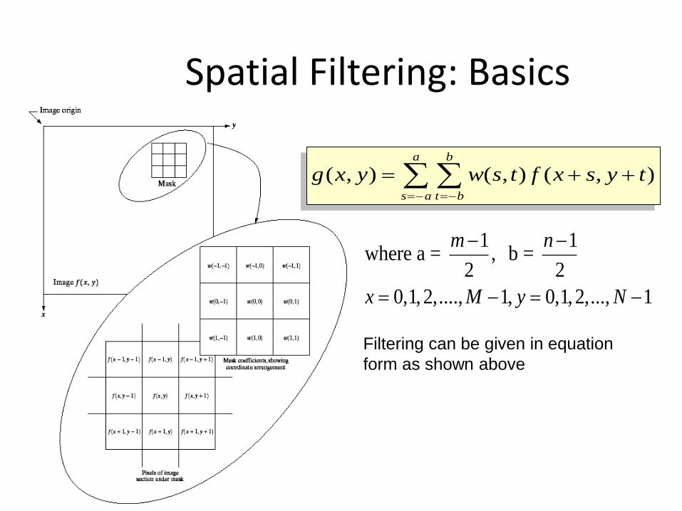
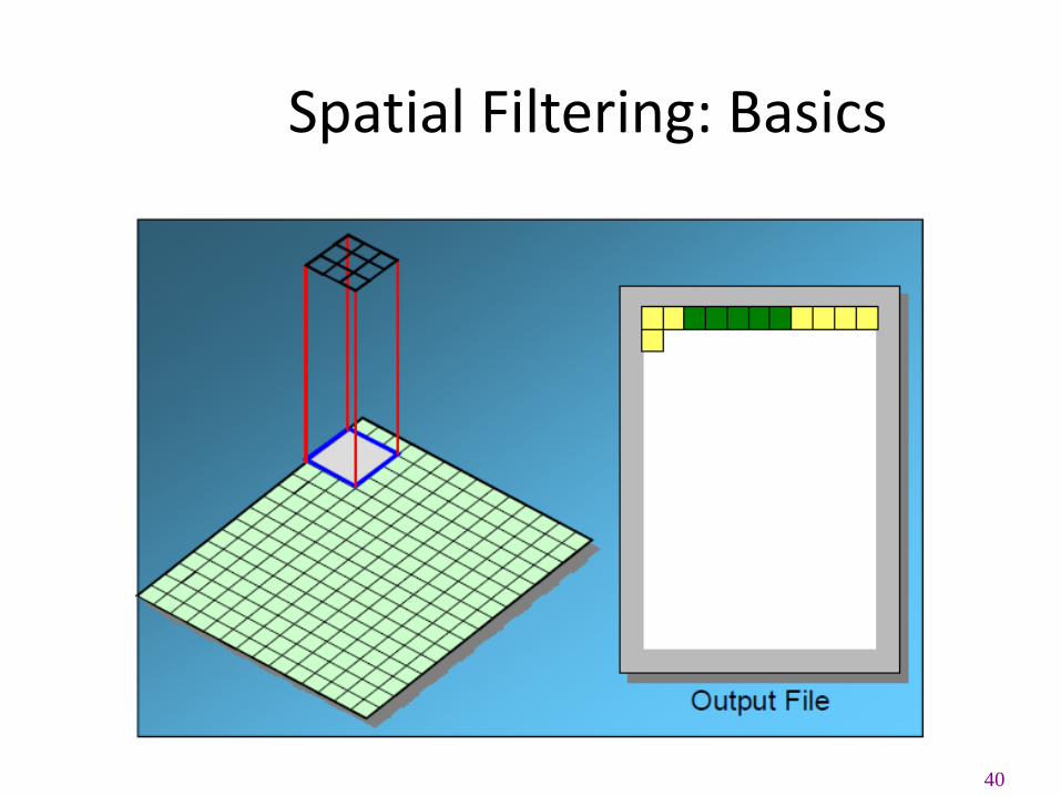
Spatial Filtering: Basics

The output intensity value at (x,y) depends not only on the inputintensity value at (x,y) but also on the specified number ofneighboring intensity values around (x,y)

Spatial masks (also called window, filter, kernel, template) are usedand convolved over the entire image for local enhancement (spatialfiltering)

The size of the masks determines the number of neighboring pixelswhich influence the output value at (x,y)

The values (coefficients) of the mask determine the nature andproperties of enhancing technique

29


1 1where a = , b =

2 2

0,1,2,...., 1, 0,1,2,..., 1

m n

x M y N

( , ) ( , ) ( , )a b

s a t b

g x y w s t f x s y t

Filtering can be given in equation

form as shown above

30


Given the 3×3 mask with coefficients: w1, w2,…, w9

The mask cover the pixels with gray levels: z1, z2,…, z9

z gives the output intensity value for the processed image (to be stored in a new array) at the location of z5 in the input image

z1 z2 z3

z4 z5 z6

z7 z8 z9

9

1 1 2 2 3 3 9 9

1

i i

i

z z w z w z w z w z w

w1 w2 w3

w4 w5 w6

w7 w8 w9

33


Neighbourhood

operations: Operate on a

larger neighbourhood of

pixels than point

operations

Origin x

y Image f (x, y)

(x, y)Neighbourhood

Neighbourhoods are mostly a

rectangle around a central

pixel

34


r s t

u v w

x y z

Origin x

y Image f (x, y)

eprocessed = v*e +

r*a + s*b + t*c +

u*d + w*f +

x*g + y*h + z*i

FilterSimple 3*3

Neighbourhoode 3*3 Filter

a b c

d e f

g h i

Original Image

Pixels

*

The above is repeated for every pixel in the original image to generate the filtered image

35


123 127 128 119 115 130

140 145 148 153 167 172

133 154 183 192 194 191

194 199 207 210 198 195

164 170 175 162 173 151

Original Image x

y

Enhanced Image x

y

36


Moving window (kernel)

scans the 3x3

neighborhood of every

pixel in the image

Original Image

37


38


39


40


41


42


Mask operation near the image border: Problem arises when part of the mask is located outside the image plane

Discard the problem pixels (e.g. 512x512 input 510x510 output if mask size is 3x3)

Zero padding: Expand the input

image by padding zeros (512x512

original image, 514x514 padded

image, 512x512 output)

Zero padding is not

recommended as it creates

artificial lines or edges on the

border

Pixel replication: We

normally use the gray

levels of border pixels to

fill up the expanded region

(for 3x3 mask). For larger

masks a border region

equal to half of the mask

size is mirrored on the

expanded region.

44

Mask operation near the border: Pixel replication

45

Smoothing Spatial Filters

Simply average all of the pixels in a neighbourhood around

a central value

1/91/9

1/9

1/91/9

1/9

1/91/9

1/9

Simple

averaging

filter

46


For blurring/noise reduction

Blurring is usually used in preprocessing steps, e.g., to remove

small details from an image prior to object extraction, or to bridge

small gaps in lines or curves

Equivalent to Low-pass spatial filtering in frequency domain

because smaller (high frequency) details are removed based on

neighborhood averaging (averaging filters)

47


1/91/9

1/91/9

1/91/9

1/91/9

1/9

Origin x

y Image f (x, y)

e = 1/9*106 + 1/9*104 + 1/9*100 + 1/9*108 + 1/9*99 + 1/9*98 + 1/9*95 + 1/9*90 + 1/9*85

= 98.3333

FilterSimple 3*3

Neighbourhood106

104

99

95

100 108

98

90 85

1/91/9

1/9

1/91/9

1/9

1/91/9

1/9

3*3 Smoothing

Filter

104 100 108

99 106 98

95 90 85

Original Image

Pixels

*

The above is repeated for every pixel in the original image to generate the smoothed image

48

Smoothing Filter: Example

original 3x3 average

49



50



51



52

Original image

Size: 500x500

Smooth by 3x3

box filter

Smooth by 5x5

box filterSmooth by 9x9

box filter

Smooth by

15x15 box filter

Smooth by

35x35 box filter

Notice how detail begins to disappear

53


Box Filter all

coefficients are

equal

Weighted Average give

more (less) weight to near

(away from) the output

location

Consider the

output pixel is

positioned at

the center

Sharpening Spatial Filters

Previously we have looked at smoothing filters which remove

fine detail

Sharpening spatial filters seek to highlight fine detail

Remove blurring from images

Highlight edges

Sharpening filters are based on spatial differentiation

Spatial Differentiation

• Let’s consider a simple 1 dimensional

example

Spatial Differentiation

A B

1st Derivative

The 1st derivative of a function is given by:

Its just the difference between subsequent

values and measures the rate of change of

the function

)()1( xfxfx

f

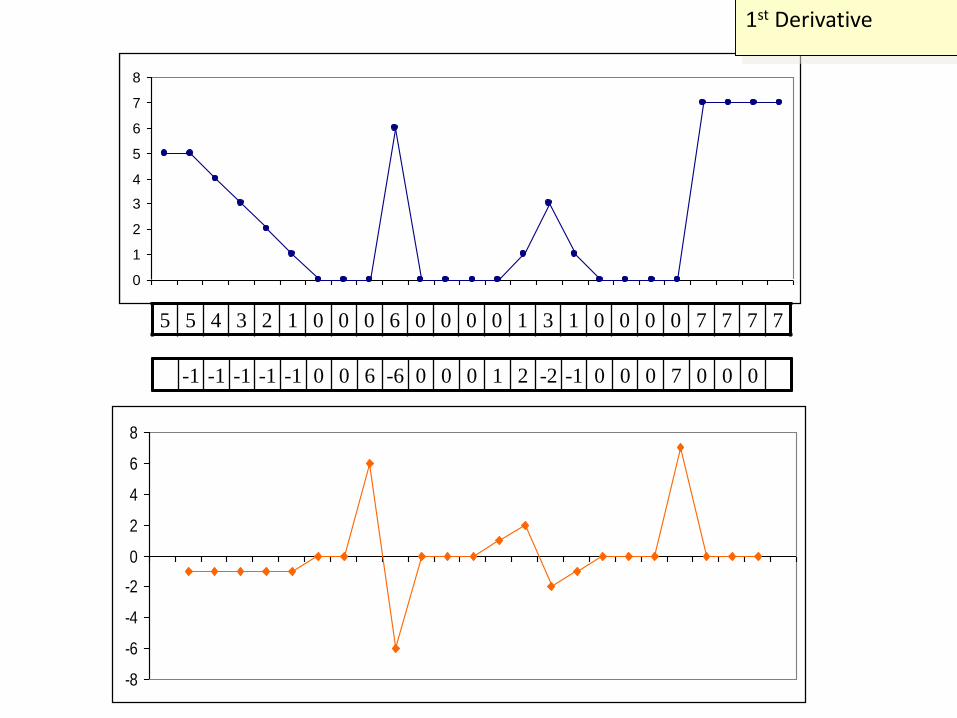
Image Strip

0

1

2

3

4

5

6

7

8

1st Derivative

-8

-6

-4

-2

0

2

4

6

8

5 5 4 3 2 1 0 0 0 6 0 0 0 0 1 3 1 0 0 0 0 7 7 7 7

-1 -1 -1 -1 -1 0 0 6 -6 0 0 0 1 2 -2 -1 0 0 0 7 0 0 0

1st Derivative

2nd Derivative

The 2nd derivative of a function is given by:

Simply takes into account the values both before and after the current value

)(2)1()1(2

2

xfxfxfx

f

Image Strip

0

1

2

3

4

5

6

7

8

5 5 4 3 2 1 0 0 0 6 0 0 0 0 1 3 1 0 0 0 0 7 7 7 7

2nd Derivative

2nd Derivative

-15

-10

-5

0

5

10

-1 0 0 0 0 1 0 6 -12 6 0 0 1 1 -4 1 1 0 0 7 -7 0 0

2nd Derivative for Image Enhancement

The 2nd derivative is more useful for image enhancement

than the 1st derivative - Stronger response to fine detail

We will come back to the 1st order derivative later on

The first sharpening filter we will look at is the Laplacian

Laplacian Filter

2

2

2

22

y

f

x

ff

),(2),1(),1(2

2

yxfyxfyxfx

f

The Laplacian is defined as follows:

),(2)1,()1,(2

2

yxfyxfyxfy

f

Laplacian Filter

So, the Laplacian can be given as follows:

),1(),1([2 yxfyxff

)]1,()1,( yxfyxf

),(4 yxf

0 1 0

1 -4 1

0 1 0

Can we implement it using a filter/ mask?

Laplacian Filter

Laplacian Filter

Applying the Laplacian to an image we get a

new image that highlights edges and other

discontinuities

Original

Image

Laplacian

Filtered Image

Laplacian

Filtered Image

Scaled for Display

Laplacian Image Enhancement

The result of a Laplacian filtering is not an

enhanced image

Laplacian

Filtered Image

Scaled for Display2

5

2

5

( , ) , 0( , )

( , ) , 0

f x y f wg x y

f x y f w

To generate the final enhanced image


In the final sharpened image edges and fine

detail are much more obvious

- =

Original

Image

Laplacian

Filtered Image

Sharpened

Image

Simplified Image Enhancement

• The entire enhancement can be combined

into a single filtering operation

),1(),1([),( yxfyxfyxf

)1,()1,( yxfyxf

)],(4 yxf

fyxfyxg 2),(),(


• The entire enhancement can be combined

into a single filtering operation

fyxfyxg 2),(),(

),1(),1(),(5 yxfyxfyxf

)1,()1,( yxfyxf0 -1 0

-1 5 -1

0 -1 0


• This gives us a new filter which does the

whole job for us in one step

0 -1 0

-1 5 -1

0 -1 0

Unsharp Masking

Use of first derivatives for image enhancement: The Gradient

• The gradient of a function f(x,y) is defined as

y

fx

f

G

G

y

xf

Gradient Operators• Most common differentiation operator is the

gradient vector.

Magnitude:

Direction:

y

x

G

G

y

yxf

x

yxf

yxf),(

),(

),(

xxyx GGGGyxf 2/122

),(

x

y

G

Gyxf 1tan),(

76

-1 -2 -1

0 0 0

1 2 1

-1 0 1

-2 0 2

-1 0 1

Extract horizontal edges

7 8 9 1 2 3

3 6 9 1 4 7

( 2 ) ( 2 )

( 2 ) ( 2 )

f z z z z z z

z z z z z z

Emphasize more the current point

(y direction)

Emphasize more the current point (x

direction) Pixel Arrangement

Gradient Operators

Extract vertical edges

Sobel Operator

Sobel Operator: Example

Sobel filters are typically used for edge

detection

An image of a

contact lens

which is

enhanced in

order to make

defects more

obvious

79

Order-Statistic Filtering

Output is based on order of gray levels in the masked area

Some simple neighbourhood operations include:

Min: Set the pixel value to the minimum in the

neighbourhood

Max: Set the pixel value to the maximum in the

neighbourhood

Median: The median value of a set of numbers is the

midpoint value in that set

80

Median Filter

• For an image, mask symmetric: 3x3, 5x5, etc.

0 2

1 2

1 2 1

2 5 3

1 3

2 2

0 1

1 2 0

2 2 4

1 0 1

Input Output

Sorted: 0,0,1,1,1,2,2,2,4

1

81

Median Filtering

Median = ? 20

Particularly effective when

The noise pattern consists of strong

impulse noise ( salt-and-pepper)

Sort the values

Determine the median

Salt and Pepper Noise

83

Median Filtering

Min/Max Filtering

Combining Spatial Enhancement Methods

Successful image enhancement is

typically not achieved using a single

operation

Rather we combine a range of

techniques in order to achieve a final

result

This example will focus on enhancing

the bone scan

Readings from Book (3rd Edn.)

• 3.3 Histogram

• 3.4 Filtering

• 3.5 Smoothing Filters

• Sharpening Filters (Chapter – 3)

• Reading Assignment

• High Boost Filtering (Chap –3.6.3)

88

Acknowledgements

Statistical Pattern Recognition: A Review – A.K Jain et al., PAMI (22) 2000

Pattern Recognition and Analysis Course – A.K. Jain, MSU

Pattern Classification” by Duda et al., John Wiley & Sons.

Digital Image Processing”, Rafael C. Gonzalez & Richard E. Woods, Addison-Wesley, 2002

Machine Vision: Automated Visual Inspection and Robot Vision”, David Vernon, Prentice Hall, 1991

www.eu.aibo.com/

Advances in Human Computer Interaction, Shane Pinder, InTech, Austria, October 2008

Mat

eria

l in

th

ese

slid

es h

as b

een

tak

en f

rom

, th

e fo

llow

ing

reso

urc

es

http://www.eu.aibo.com/

Lecture # 3 Histogram Matching Spatial...

Documents

Transcript of Lecture # 3 Histogram Matching Spatial...