Liquefaction IIT Roorkee Dec 26 2012

Soil Liquefaction: Experimental and Field Investigations

Prof. T. G. SitharamDepartment of Civil Engineering and Chairman, CiSTUP

Indian Institute of Science, Bangalore-560 012.

IIT Roorkee, 26th Dec 2012

Jan 26 2001

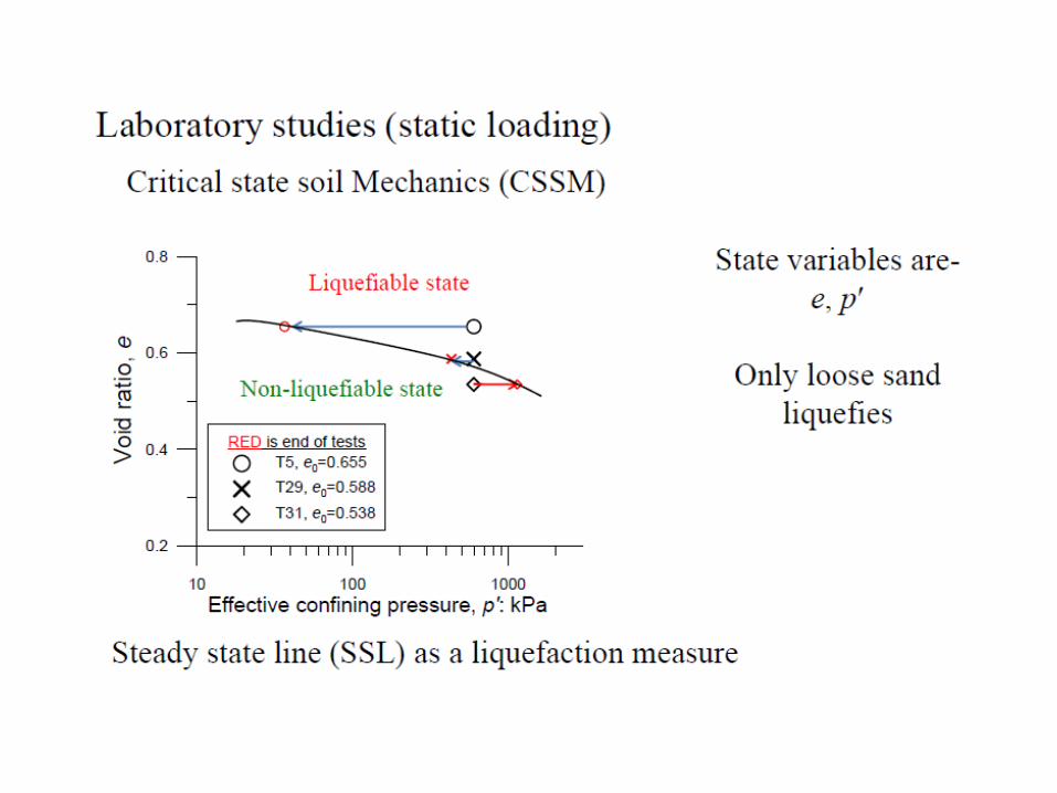
Soil Liquefaction Introduced by Casagrande in 1936 The effective strength of saturated

cohesion less soil is reduced drastically due to sudden loading.

wu

w' uσσstressEffective

φtanuστ

φtanστstrengthShear

w

'

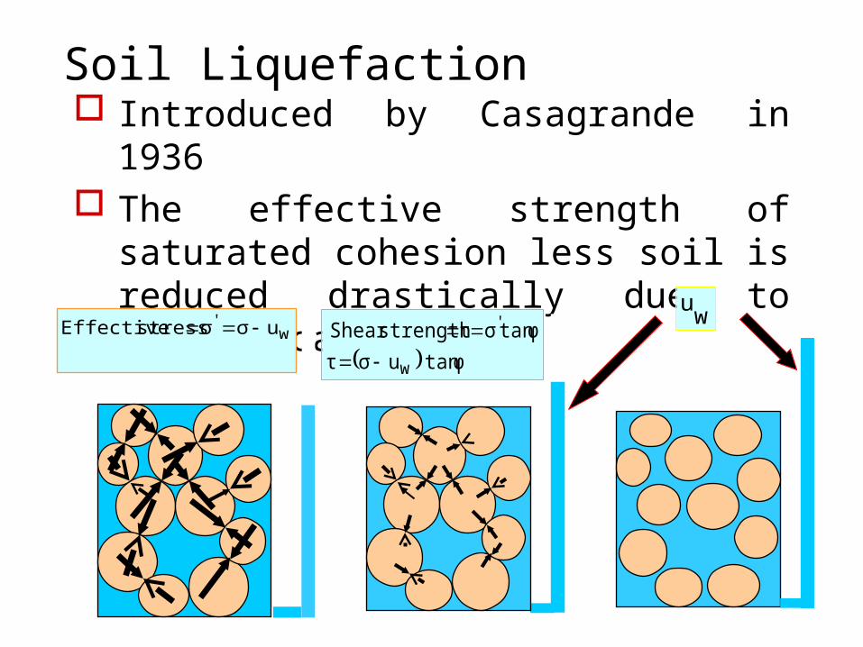
Liquefaction process

Liquefaction occurs when solid material transforms into liquid state due to the increased pore pressure

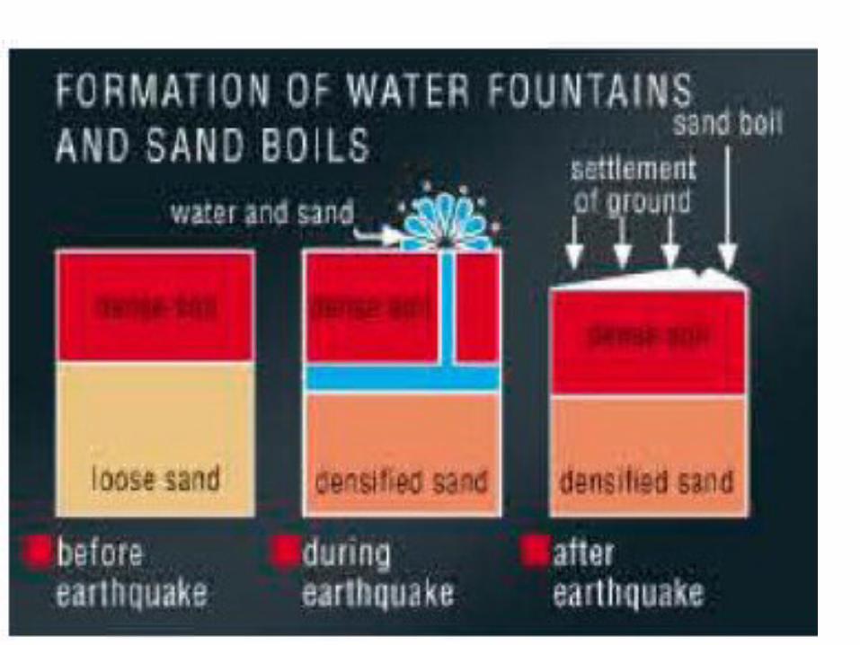
Issue of liquefaction and ground failure

Northridge, 1994

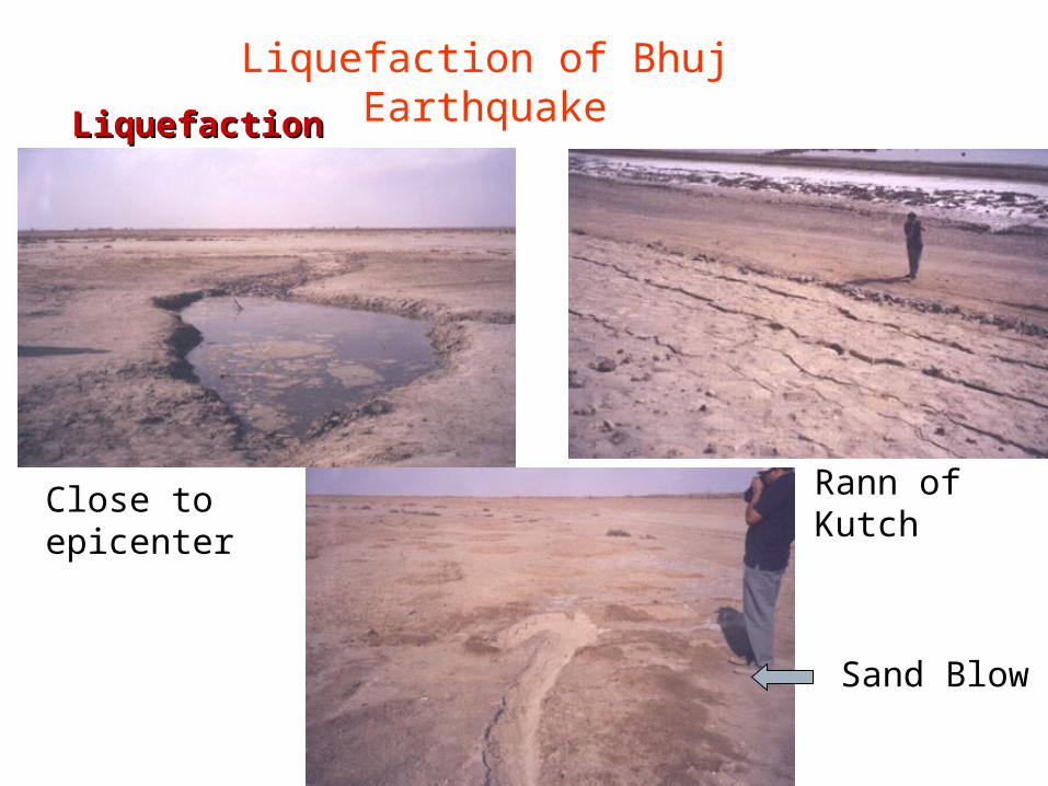
Liquefaction of Bhuj Earthquake

Close to epicenter

LiquefactionLiquefaction

Rann of Kutch

Sand Blow

fjfg

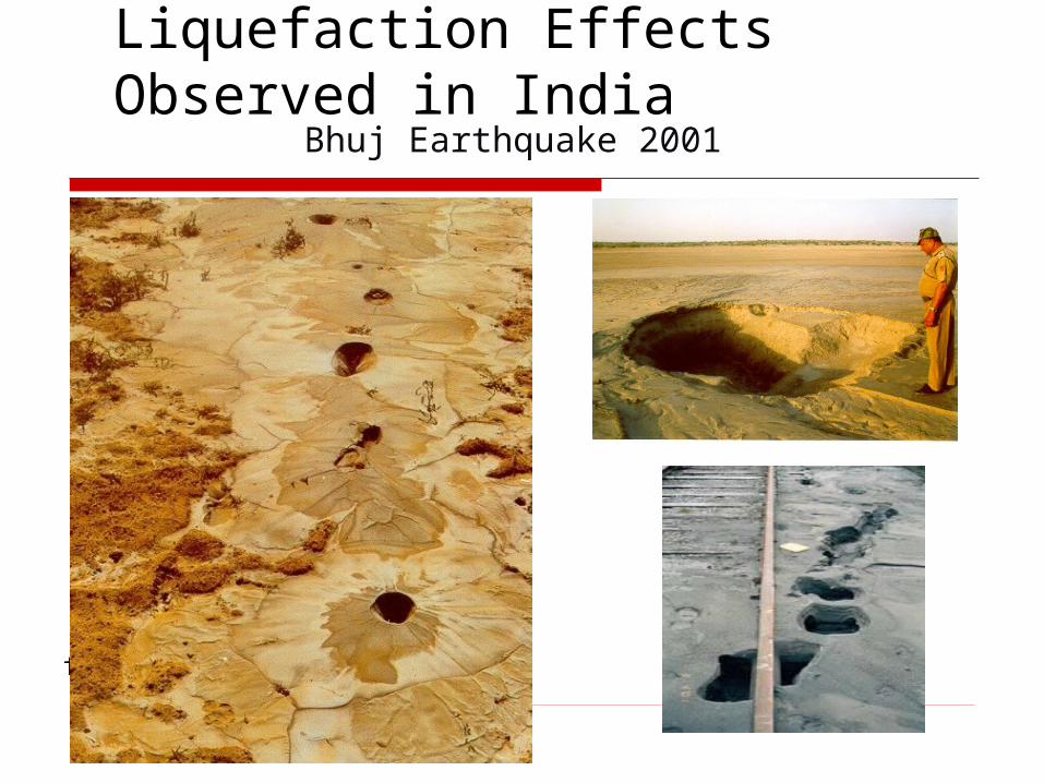
Liquefaction Effects Observed in India

Bhuj Earthquake 2001

fjfg

Satellite image of Liquefaction at Bhuj

Jan 15, 2001

Jan 31, 2001

http://earthobservatory.nasa.gov

More than 10,000 sq km area was liquefied during Bhuj earthquake

Liquefaction during Bhuj Earthquake 2001

Field investigations have found abundant evidence of mud volcanos, sand boils, and fissures from which salty ground water erupted over an area exceeding 10,000 square kilometers. Evidence of the expelled water can also be seen on the MISR images.

Pre -January 15 Post January 31, 2001

Liss III FCC images

"false-color“ (MISR) Images

SITHARAM

9

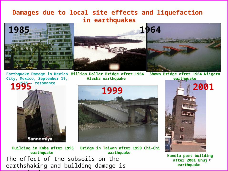
Million Dollar Bridge after 1964 Alaska earthquake

Showa Bridge after 1964 Niigata earthquake

Building in Kobe after 1995 earthquake

1964

1995 1999 2001

Bridge in Taiwan after 1999 Chi-Chi earthquake

Kandla port building after 2001 Bhuj earthquake

Damages due to local site effects and liquefaction in earthquakes

Earthquake Damage in Mexico City, Mexico, September 19, 1985 - resonance

1985

The effect of the subsoils on the earthshaking and building damage is emphasized.

10

Guerro EQ 1985 – Mexico city, Mexico Spitak EQ 1988 – Leninakan, Armenia (Soviet U) Loma Prieta EQ 1989 – San Francisco bay area, US Kobe EQ 1995 – coastal areas of city, Japan Kocaeli EQ 1999 – Adapazari, Turkey Erzincan 1992 – Turkey, resonance Bhuj EQ 2001 – Bhuj, India-Liquefaction Christchurch , New Zealand Earthquake 2010

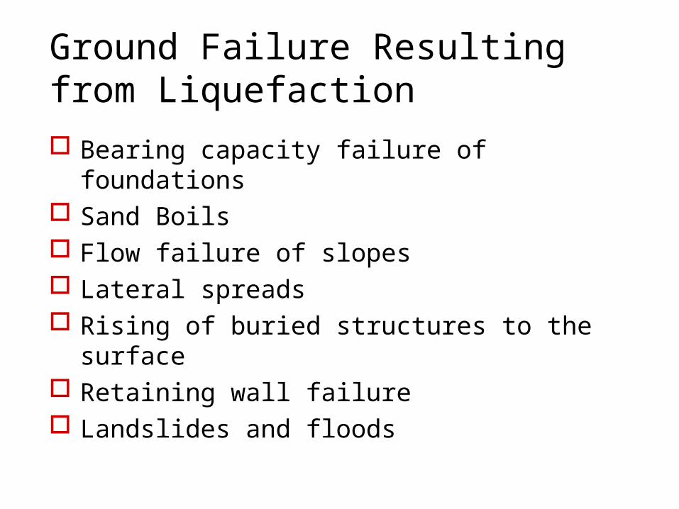
Ground Failure Resulting from Liquefaction

Bearing capacity failure of foundations Sand Boils Flow failure of slopes Lateral spreads Rising of buried structures to the

surface Retaining wall failure Landslides and floods

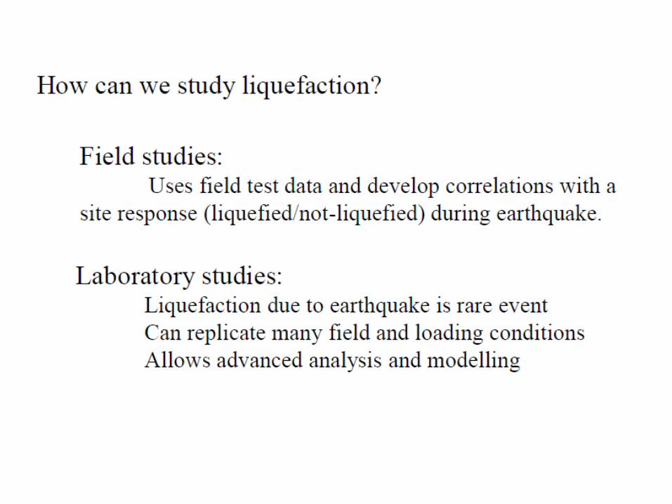
Liquefaction – Susceptibility and Potential

Liquefaction Susceptibility Evaluation is done by considering the soil

properties alone

Earthquake loading is not taken into account

Liquefaction Potential Both soil properties and earthquake

loading are considered

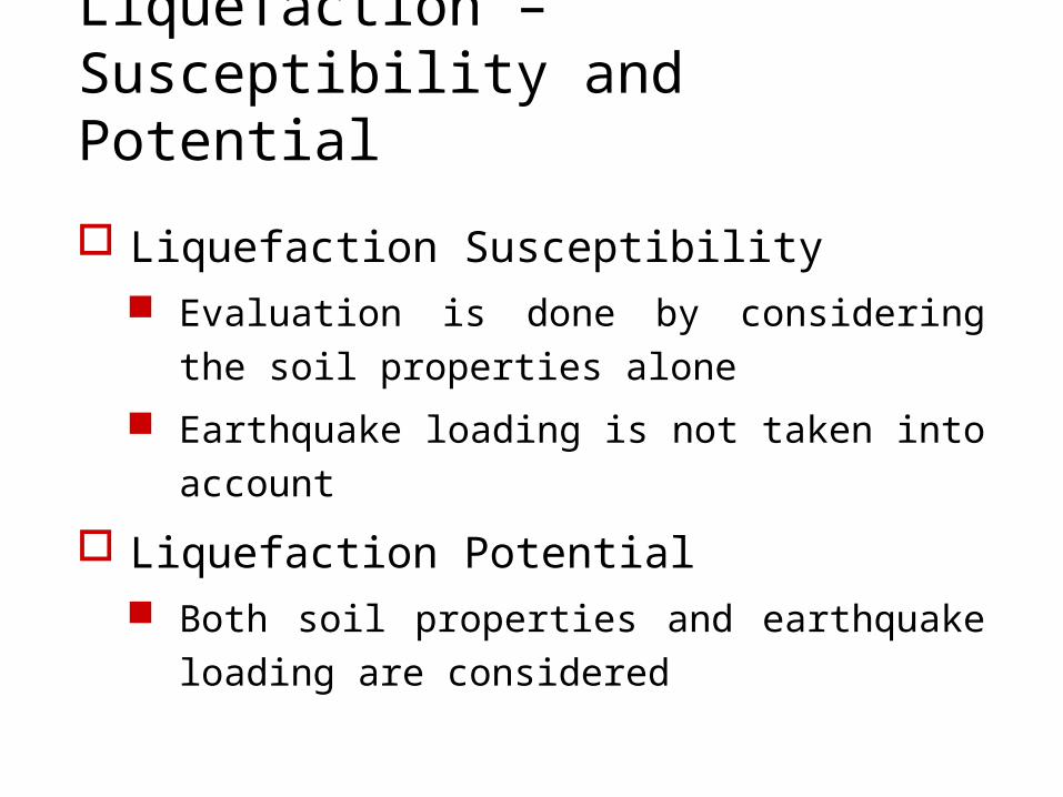
Liquefaction Susceptibility Based on Soil Properties

Age of the soil

Index properties of soil

Shape of particles

Relative density of soil

Permeability of soil

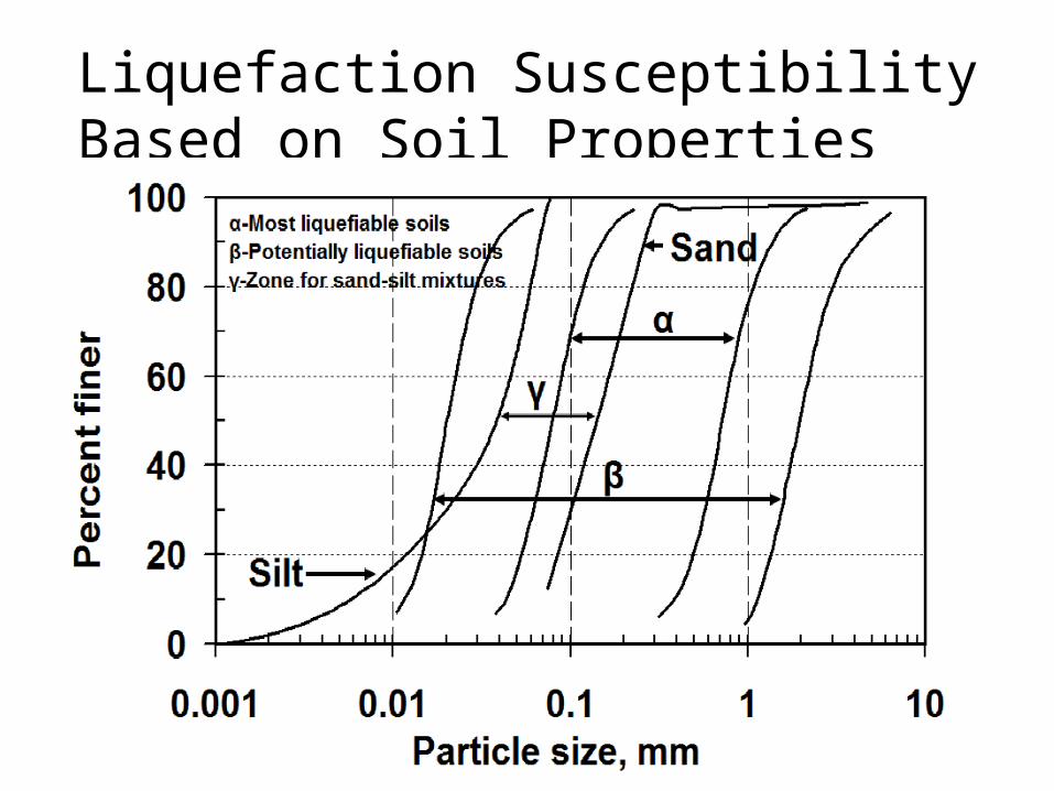
Liquefaction Susceptibility Index Properties – Chinese Criteria

w = 0.87LL

Saturated moisture content, w (%)

NON-LIQUEFIABLE SOIL: w < 0.87LL or LL > 33.5 or Clay fraction > 20% or Plasticity Index > 13

LL = 33.5

POTENTIALLY LIQUEFIABLE SOIL IF: Clay fraction (0.005 mm) is less than 20% Plasticity Index is less than or equal to 13.

Liq

uid

Lim

it, L

L

60

50

40

30

20

10

0 0 20 40 60 80

Chinese Criteria Adapted to ASTM Definitions of Soil Properties (Perlea et al., 1999)

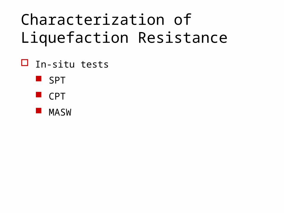
Characterization of Liquefaction Resistance

In-situ tests

SPT

CPT

MASW

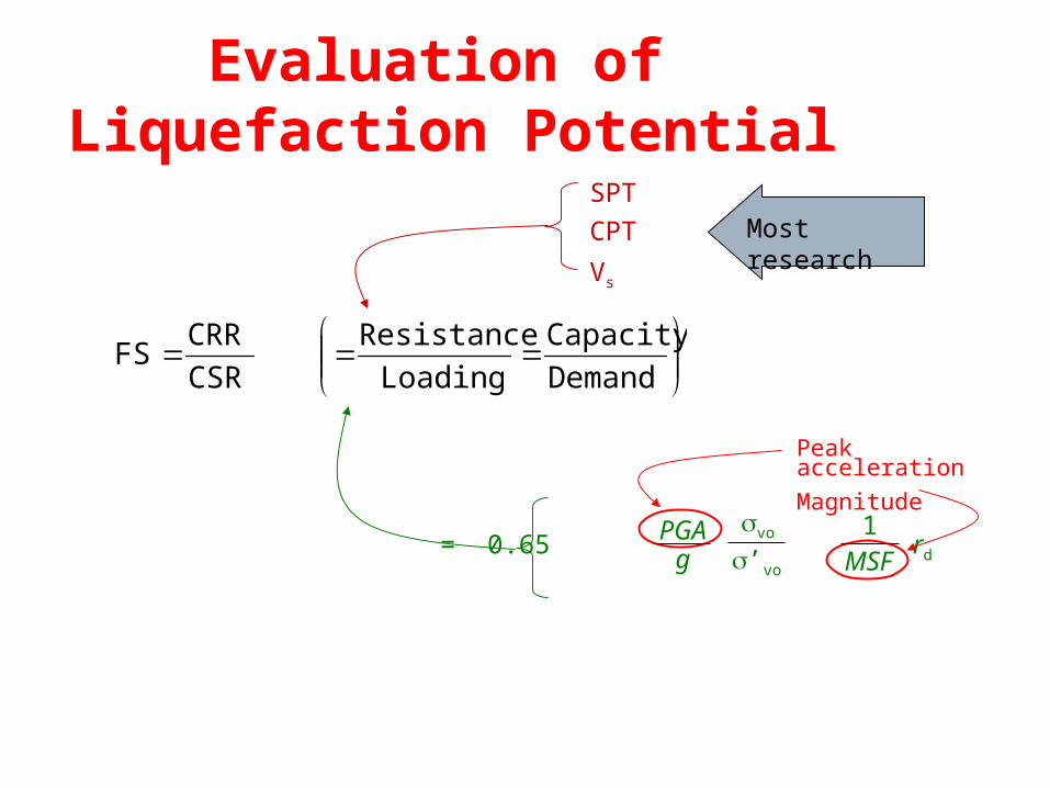
Evaluation of Liquefaction Potential

Peak acceleration

Magnitude

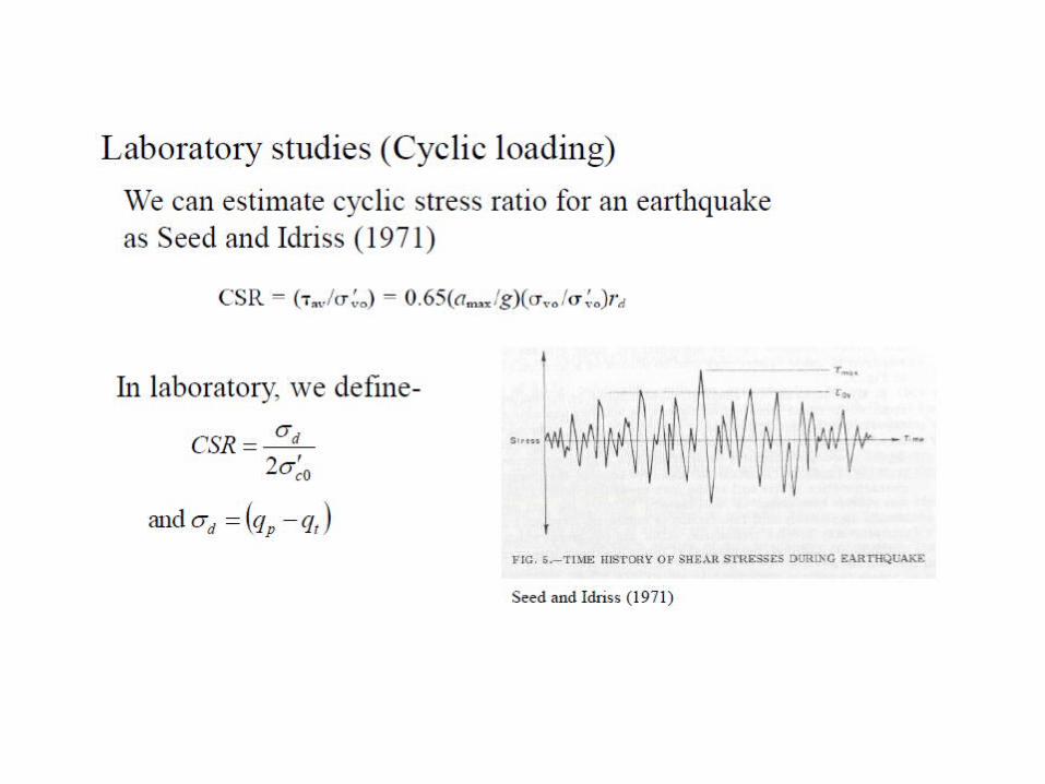
= 0.65 rdPGA

g ’vo

vo 1MSF

Demand

Capacity

Loading

Resistance

CSR

CRRFS

SPT

CPT

Vs

Most research

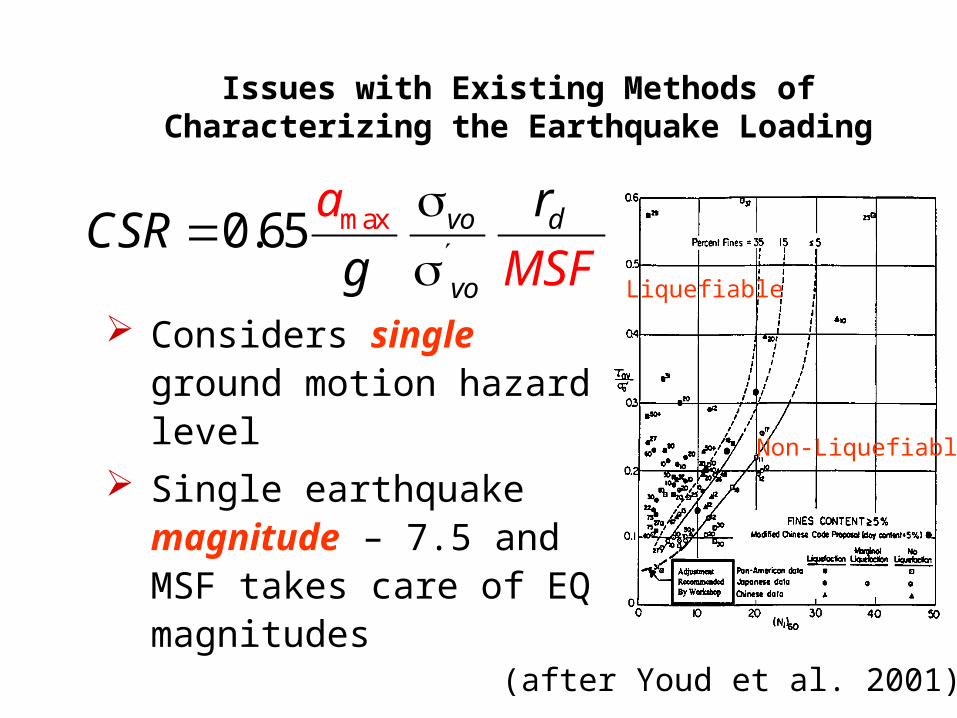
Issues with Existing Methods of Characterizing the Earthquake Loading

Considers single ground motion hazard level

Single earthquake magnitude – 7.5 and MSF takes care of EQ magnitudes

max0.65 vo d

vo

rCSR

g

a

MSF

(after Youd et al. 2001)

Liquefiable

Non-Liquefiable

Depth Reduction Factor - rd

The Shear stress at a depth “h” is calculated by assuming that the soil column is rigid.

rd is introduced to account for the flexibility of soils

maxrigid body

ah

g

ddeformable soil rigid bodyr

Seed and Idriss, 1971

rd – Cetin and Seed (2004)

Evaluates rd as a function of Depth Earthquake magnitude Ground acceleration Soil Stiffness

*,12

*,12

*max ,12

0.341( 0.0785 7.586)*

max ,12 *max ,12

0.341(0.0785 7.586)

23.013 2.949 0.999 0.05251

16.258 0.201( , , , )

23.013 2.949 0.999 0.05251

16.258 0.201

s

r

s

w sd V

sdw s

V

a M V

er d Mw a V

a M V

e

d

Magnitude Reduction Factor

Earthquake Magnitude, MW

Mag

nitu

de S

calin

g Fa

ctor

, MS

F

Youd and Noble, 1997

2.24

2.56

10

W

MSFM

Youd et al., 2001

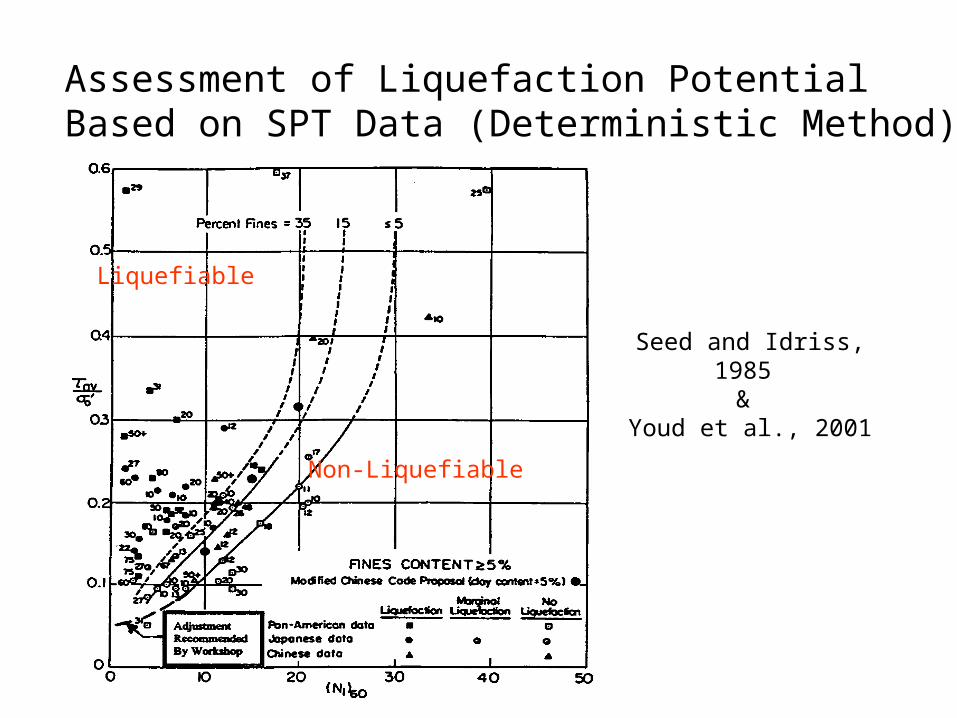
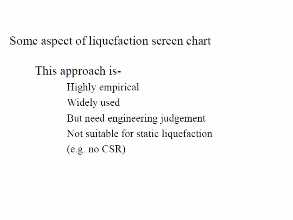
Assessment of Liquefaction Potential Based on SPT Data (Deterministic Method)

Liquefiable

Non-Liquefiable

Seed and Idriss, 1985

& Youd et al., 2001

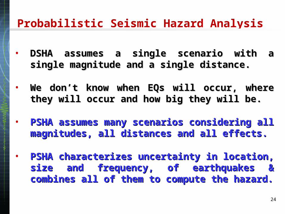
Probabilistic Seismic Hazard Analysis

24

• DSHA assumes a single scenario with a DSHA assumes a single scenario with a single magnitude and a single distance.single magnitude and a single distance.

• We don’t know when EQs will occur, where We don’t know when EQs will occur, where they will occur and how big they will be.they will occur and how big they will be.

• PSHA assumes many scenarios considering PSHA assumes many scenarios considering all magnitudes, all distances and all effects.all magnitudes, all distances and all effects.

• PSHA characterizes uncertainty in location, PSHA characterizes uncertainty in location, size and frequency, of earthquakes & size and frequency, of earthquakes & combines all of them to compute the hazard.combines all of them to compute the hazard.

Steps Taken to Evaluate the Liquefaction Potential

Peak horizontal acceleration (PHA) values at bed rock level was evaluated using Probabilistic seismic hazard analysis.

Since site characterization data was not available, the surface level peak ground acceleration (PGA) were evaluated for four NEHRP site classes (Site class A to D).

Deaggregated the seismic hazard with respect to magnitude

Evaluation of liquefaction return period – based on PGA values.

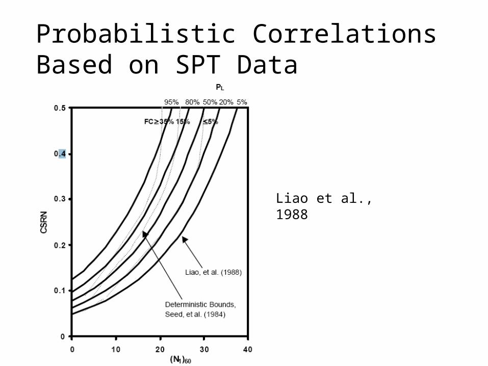
Probabilistic Correlations Based on SPT Data

Liao et al., 1988

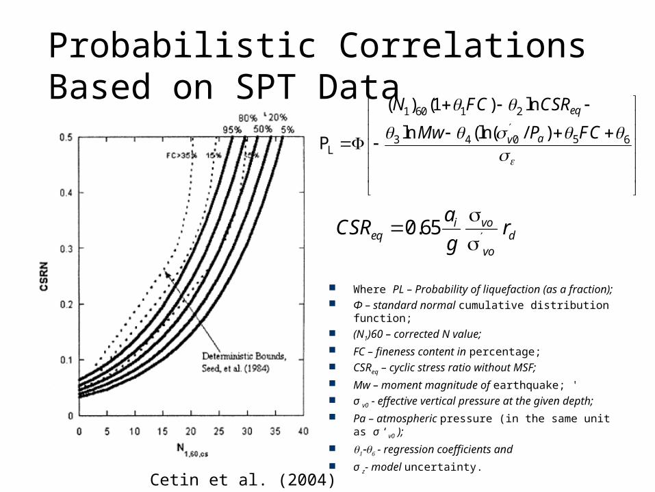
Probabilistic Correlations Based on SPT Data

Cetin et al. (2004)

1 60 1 2

53 4 0 6L

( ) (1 ) ln

ln (ln( / )P

eq

av

N FC CSR

Mw P FC

0.65 i voeq d

vo

aCSR r

g

Where PL – Probability of liquefaction (as a fraction);

Φ – standard normal cumulative distribution function;

(N1)60 – corrected N value; FC – fineness content in percentage; CSReq – cyclic stress ratio without MSF; Mw – moment magnitude of earthquake; ' σ v0 - effective vertical pressure at the given

depth; Pa – atmospheric pressure (in the same unit as σ

‘v0 );

- regression coefficients and

σ z- model uncertainty.

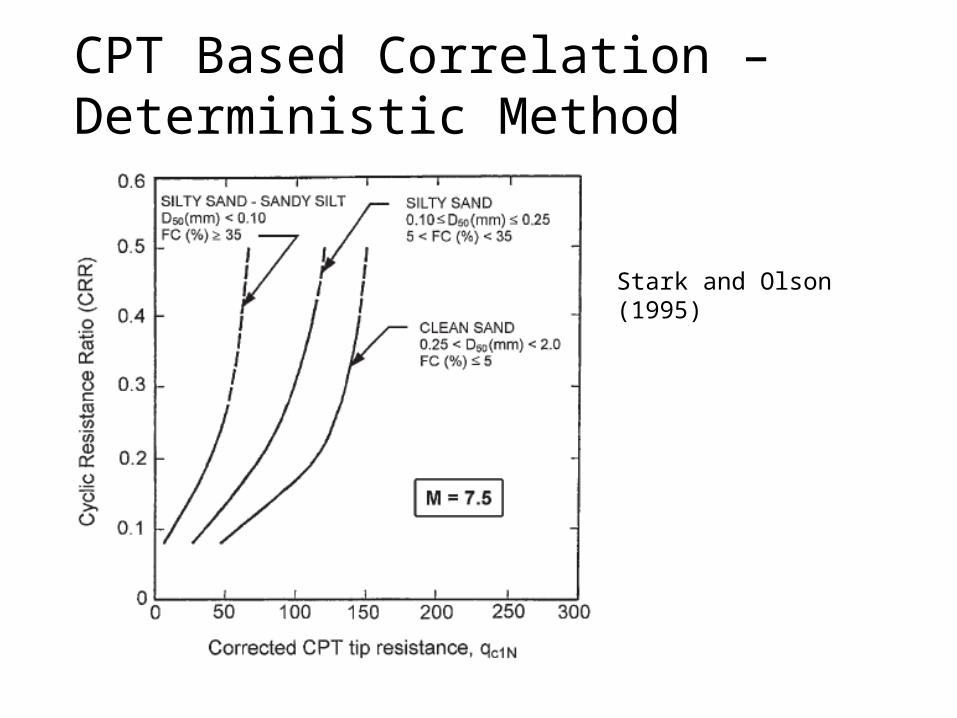
CPT Based Correlation – Deterministic Method

Stark and Olson (1995)

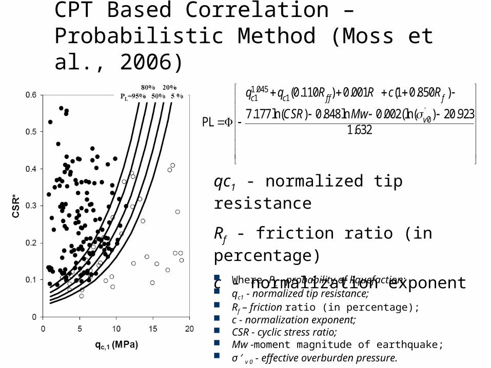
CPT Based Correlation – Probabilistic Method (Moss et al., 2006)

1.0451 1

0

(0.110 ) 0.001 (1 0.850 )

7.177ln( ) 0.848ln 0.002(ln( ) 20.923PL

1.632

c c f f f

v

q q R R c R

CSR Mw

qc1 - normalized tip resistance

Rf - friction ratio (in percentage)

c - normalization exponent Where PL - probability of liquefaction; qc1 - normalized tip resistance; Rf – friction ratio (in percentage); c - normalization exponent; CSR - cyclic stress ratio; Mw -moment magnitude of earthquake; σ ′ v 0 - effective overburden pressure.

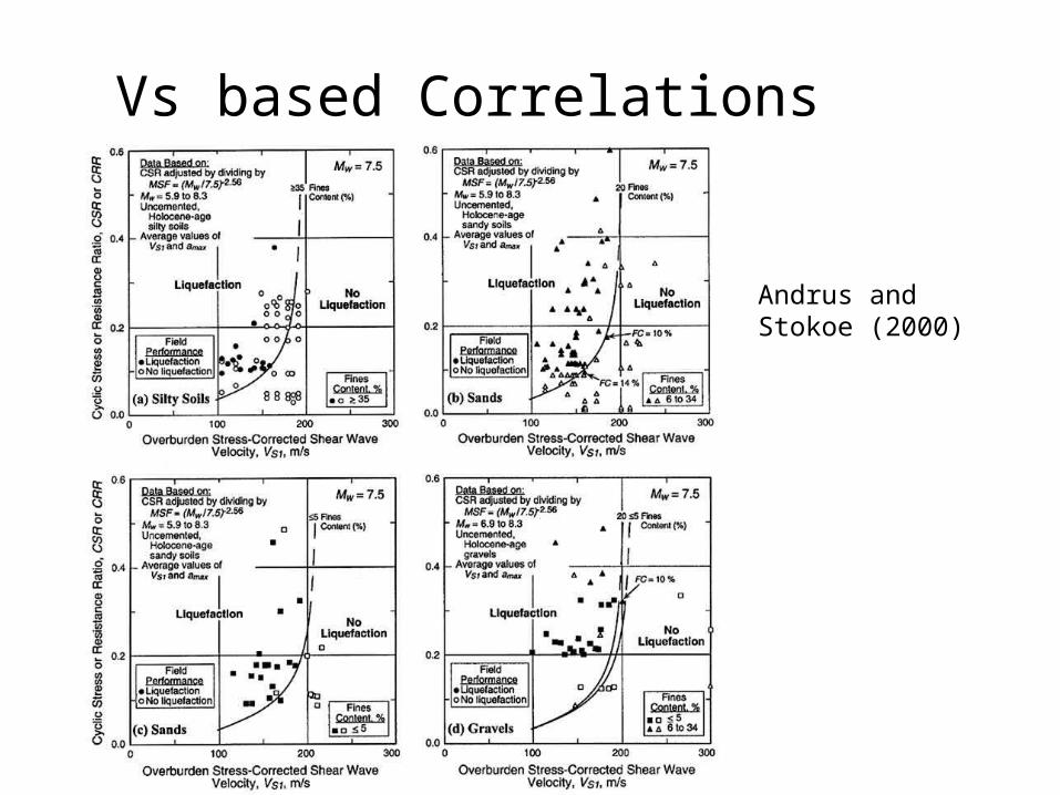
Vs based Correlations

Andrus and Stokoe (2000)

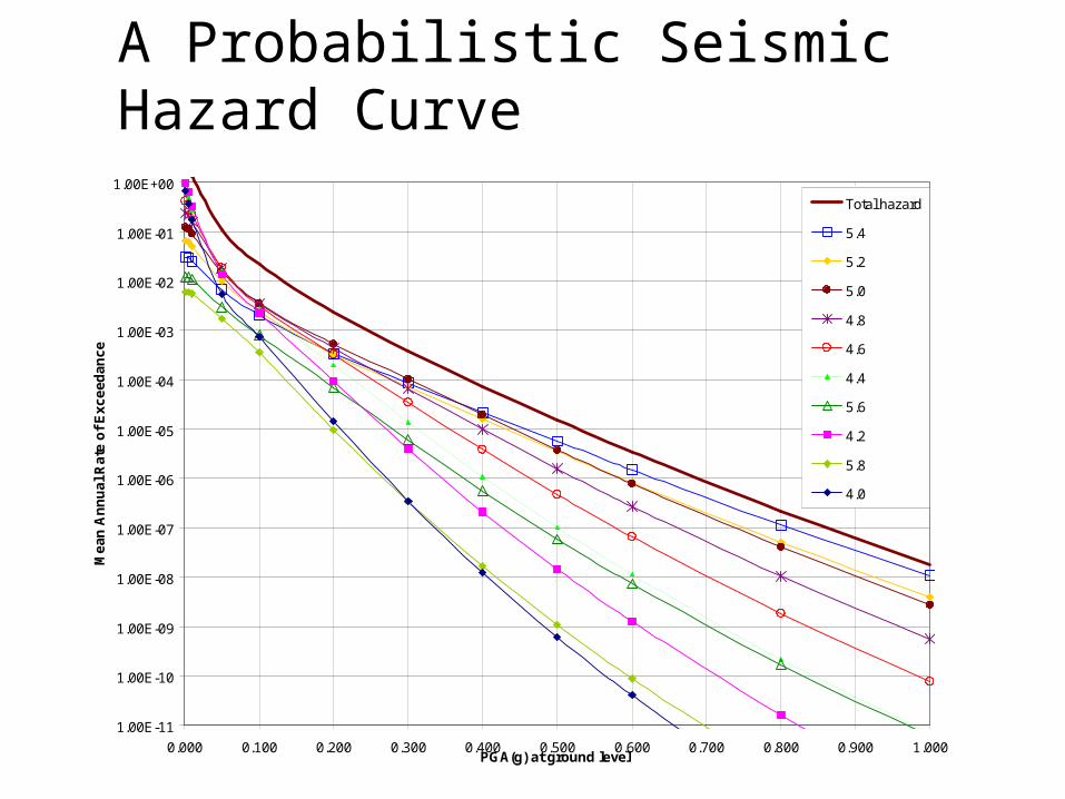
A Probabilistic Seismic Hazard Curve

1.00E-11

1.00E-10

1.00E-09

1.00E-08

1.00E-07

1.00E-06

1.00E-05

1.00E-04

1.00E-03

1.00E-02

1.00E-01

1.00E+00

0.000 0.100 0.200 0.300 0.400 0.500 0.600 0.700 0.800 0.900 1.000PGA(g) at ground level

Me

an

An

nu

al

Ra

te o

f E

xc

ee

da

nc

e

Total hazard

5.4

5.2

5.0

4.8

4.6

4.4

5.6

4.2

5.8

4.0

Performance-Based EarthquakePerformance-Based EarthquakeEngineeringEngineering

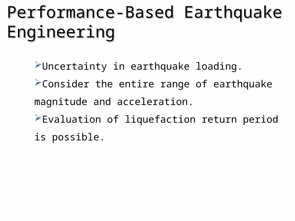
Uncertainty in earthquake loading.

Consider the entire range of earthquake

magnitude and acceleration.

Evaluation of liquefaction return period is

possible.

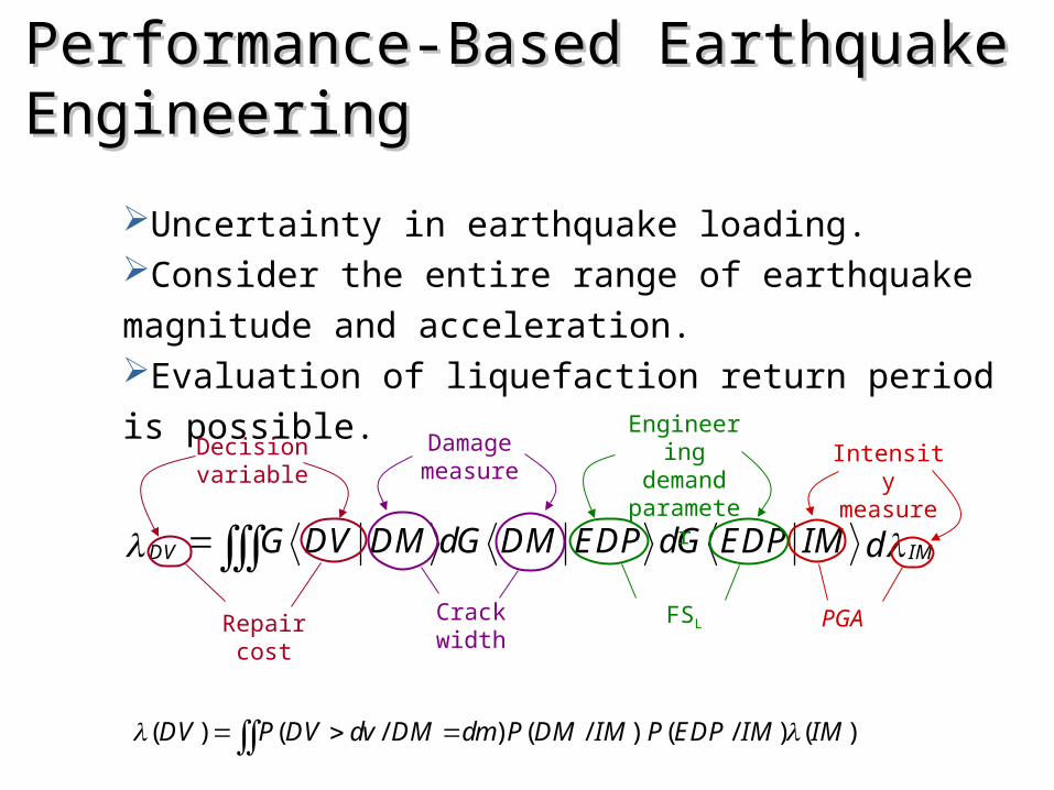
Performance-Based EarthquakePerformance-Based EarthquakeEngineeringEngineering

Uncertainty in earthquake loading.Consider the entire range of earthquake magnitude and acceleration.Evaluation of liquefaction return period is possible.

DV IMG DV DM dG DM EDP dG EDP IM d

Intensity measure

Engineering demand parameter

Damage measure

Decision variable

Repair cost

Crack width

FSL PGA

( ) ( / ) ( / ) ( / ) ( )DV P DV dv DM dm P DM IM P EDP IM IM

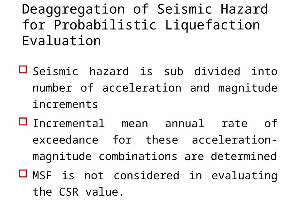
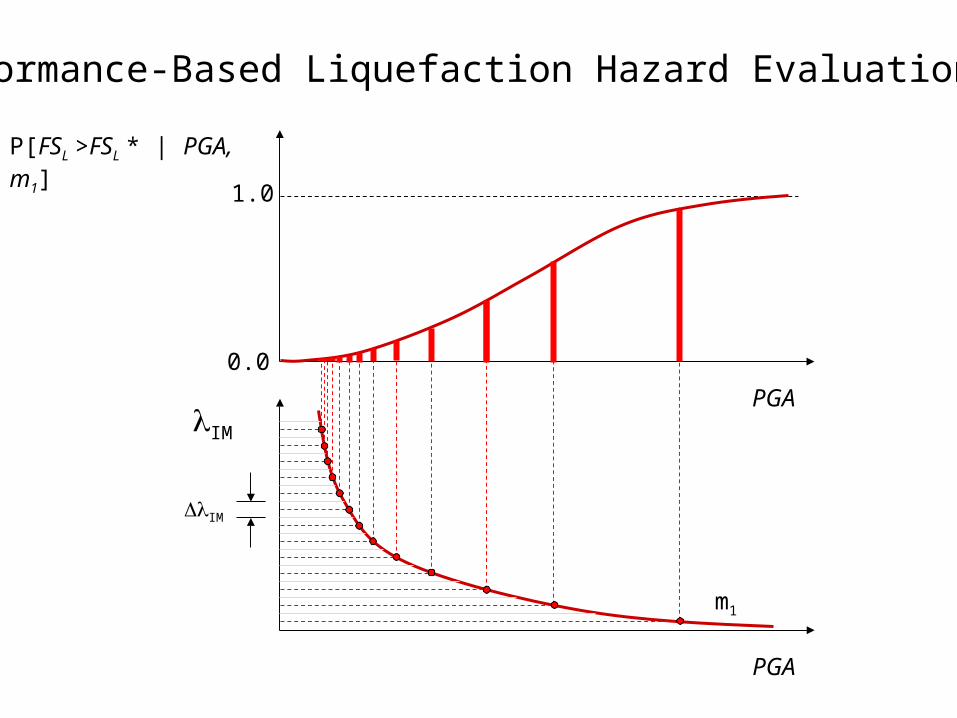
Deaggregation of Seismic Hazard for Probabilistic Liquefaction Evaluation

Seismic hazard is sub divided into

number of acceleration and magnitude

increments

Incremental mean annual rate of

exceedance for these acceleration-

magnitude combinations are determined

MSF is not considered in evaluating the

CSR value.

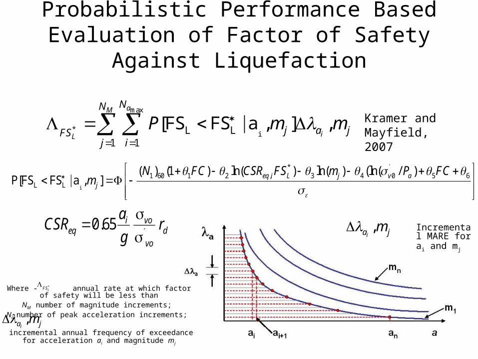
Probabilistic Performance Based Evaluation of Factor of Safety Against Liquefaction

0.65 i voeq d

vo

aCSR r

g

max

*iL L

1 1

[FS FS a , ] ,aM

iL

NN

j a jFSj i

P m m

i

*1 60 1 2 , 3 4 0 5 6

L L

( ) (1 ) ln( ) ln( ) (ln( / )P[FS FS a , ] eq i L j v a

j

N FC CSR FS m P FCm

,ia jm

Kramer and Mayfield, 2007

Incremental MARE for ai and mj

Where - annual rate at which factor of safety will be less than

NM number of magnitude increments; Na number of peak acceleration increments;

incremental annual frequency of exceedance for

acceleration ai and magnitude mj

*LFS

,ia jm

IM

PGA

PGA

P[FSL >FSL * | PGA, m1] 1.0

0.0

Performance-Based Liquefaction Hazard Evaluation

IM

m1

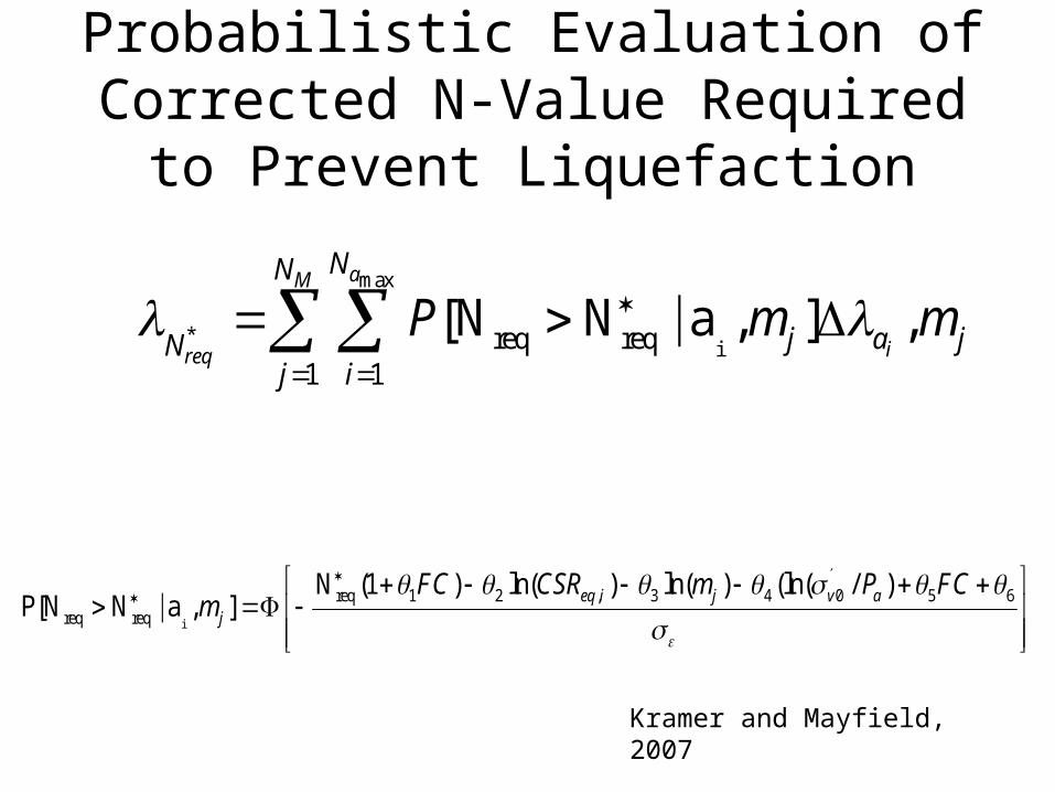
Probabilistic Evaluation of Corrected N-Value Required to

Prevent Liquefaction

max

*ireq req

1 1

[N N a , ] ,aM

ireq

NN

j a jNj i

P m m

i

req 1 2 , 3 4 0 5 6req req

N (1 ) ln( ) ln( ) (ln( / )P[N N a , ] eq i j v a

j

FC CSR m P FCm

Kramer and Mayfield, 2007

Case Study - Gujarat

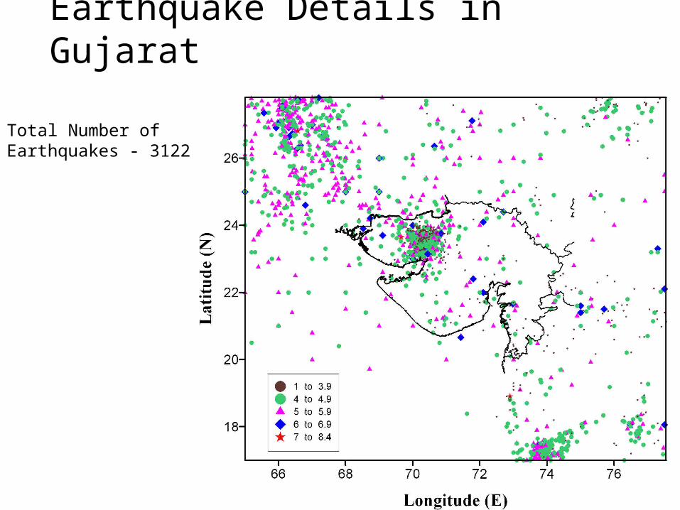
Earthquake Details in Gujarat

Total Number of Earthquakes - 3122

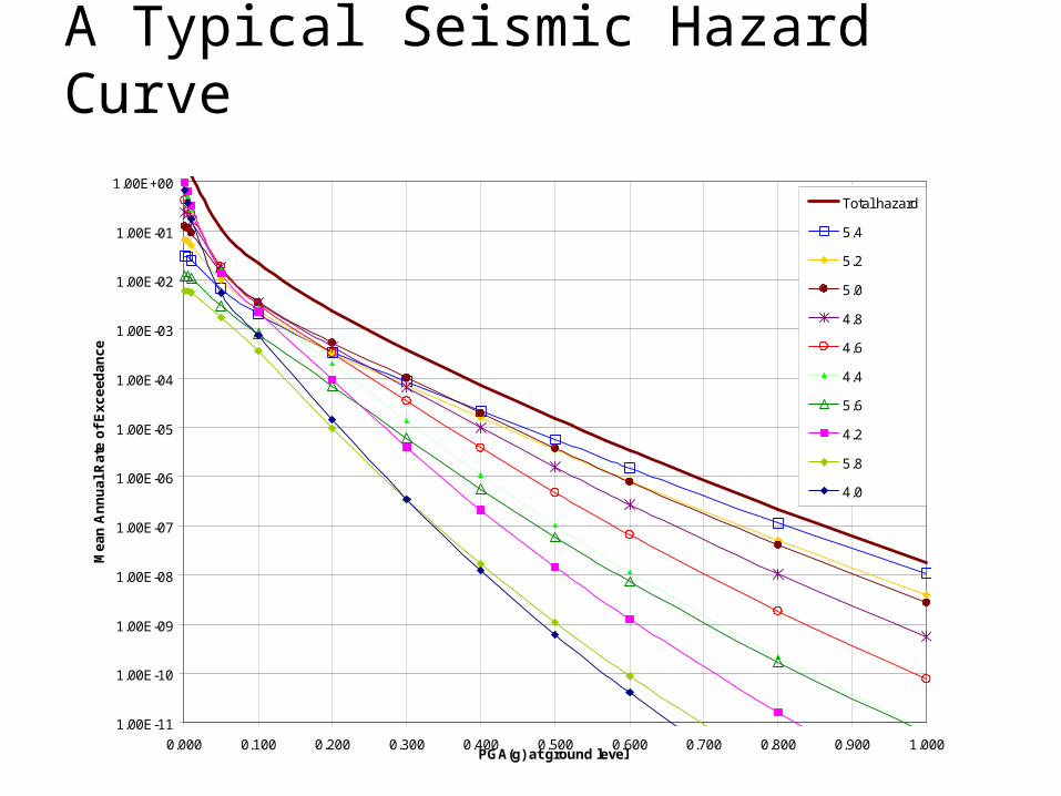
A Typical Seismic Hazard Curve

1.00E-11

1.00E-10

1.00E-09

1.00E-08

1.00E-07

1.00E-06

1.00E-05

1.00E-04

1.00E-03

1.00E-02

1.00E-01

1.00E+00

0.000 0.100 0.200 0.300 0.400 0.500 0.600 0.700 0.800 0.900 1.000PGA(g) at ground level

Me

an

An

nu

al

Ra

te o

f E

xc

ee

da

nc

e

Total hazard

5.4

5.2

5.0

4.8

4.6

4.4

5.6

4.2

5.8

4.0

Liquefaction Hazard Curves

1.E-08

1.E-06

1.E-04

1.E-02

0 5 10 15 20 25 30 35 40

Corrected N Value

An

nu

al

rae

of

Ex

ce

ed

an

ce

Bhuj

Jamnagar

Rajkot

Ahmadabad

Surat

Vadodara

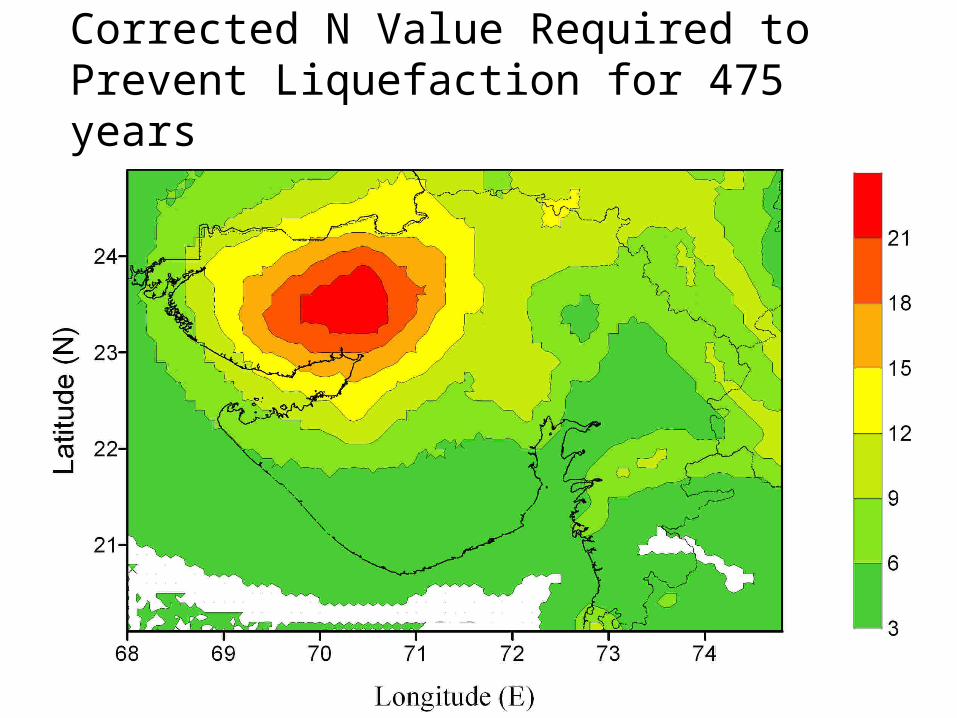
Corrected N Value Required to Prevent Liquefaction for 475 years

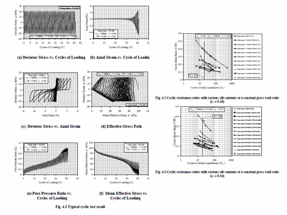
Effect of fines on Liquefaction

0

0.05

0.1

0.15

0.2

0.25

1 10 100 1000Cycles to Initial Liquefaction (N L )

Cyc

lic

Str

ess

Rat

io (

CSR

)

Clean Sand (CRR=0.184)

Clean Sand+5%Silt (CRR=0.2025)












Silt (CRR=0.1108)σ'3c = 100kPa, f = 0.1Hz, RD c = 53%

N = 20

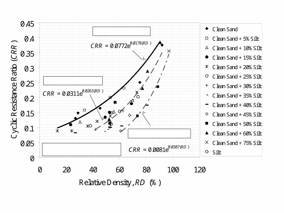
CRR = 0.0772e0.0178(RD )

CRR = 0.0311e0.0263(RD )

CRR = 0.0081e0.0387(RD )

0

0.05

0.1

0.15

0.2

0.25

0.3

0.35

0.4

0.45

0 20 40 60 80 100 120

Relative Density, RD (%)

Cyc

lic

Res

ista

nce

Rat

io (

CR

R)

Clean Sand

Clean Sand + 5%Silt

Clean Sand + 10%SIlt

Clean Sand + 15%Silt










Silt

Upper Bound Curve

Mean Curve

Lower Bound Curve

σ'3c = 100kPa, f = 0.1Hz

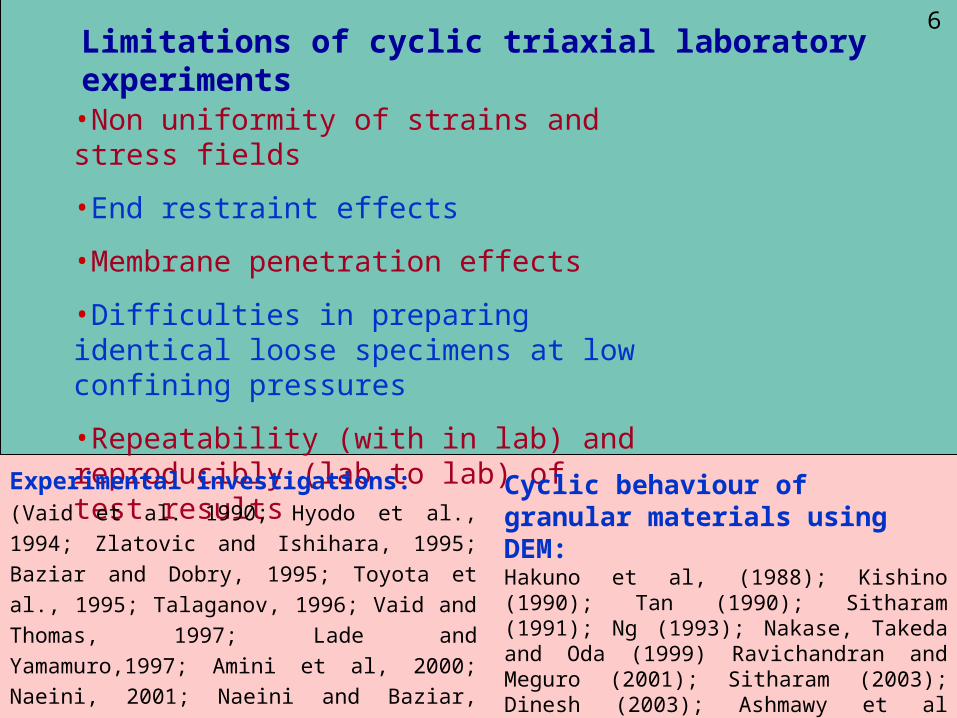
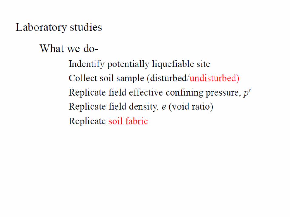
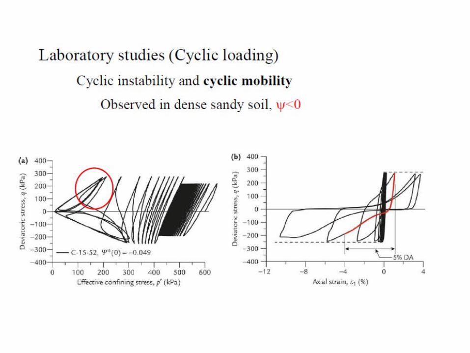
Limitations of cyclic triaxial laboratory experiments

•Non uniformity of strains and stress fields

•End restraint effects

•Membrane penetration effects

•Difficulties in preparing identical loose specimens at low confining pressures

•Repeatability (with in lab) and reproducibly (lab to lab) of test results

Experimental investigations:(Vaid et al. 1990; Hyodo et al., 1994; Zlatovic and

Ishihara, 1995; Baziar and Dobry, 1995; Toyota et al.,

1995; Talaganov, 1996; Vaid and Thomas, 1997; Lade

and Yamamuro,1997; Amini et al, 2000; Naeini, 2001;

Naeini and Baziar, 2004; Govida Raju, 2005)

Cyclic behaviour of granular materials using DEM: Hakuno et al, (1988); Kishino (1990); Tan (1990); Sitharam (1991); Ng (1993); Nakase, Takeda and Oda (1999) Ravichandran and Meguro (2001); Sitharam (2003); Dinesh (2003); Ashmawy et al (2003); Roberto (2004); Mourad Zeghal and Usama El Shamy (2005).

6

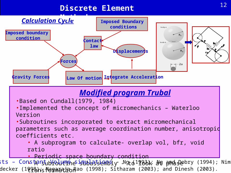
Calculation Cycle

t

f

f

kft

k

n

ft

n

c,

n

t

f

f

kft

k

n

ft

n

c,

n

kft

k

n

ft

n

c,

n

ftk

n

ft

n

c,

n

tk

n

ft

n

c, c,

n

Imposed boundary condition

Forces

Gravity Forces Law Of motion Integrate Acceleration

Displacements

Contact law

Imposed Boundary conditions

Modified program Trubal•Based on Cundall(1979, 1984)•Implemented the concept of micromechanics – Waterloo Version•Subroutines incorporated to extract micromechanical parameters such as average coordination number, anisotropic coefficients etc.

• A subprogram to calculate- overlap vol, bfr, void ratio• Periodic space boundary condition• A subroutine subassembly - to look at phase transformation• Plot files were developed using java

Discrete Element Method

Undrained tests – Constant Volume simulations - Ng (1993); Ng and Dobry (1994); Nimbkar (1996); Dubujet and Dedecker (1998); Nagaraja Rao (1998); Sitharam (2003); and Dinesh (2003).

12

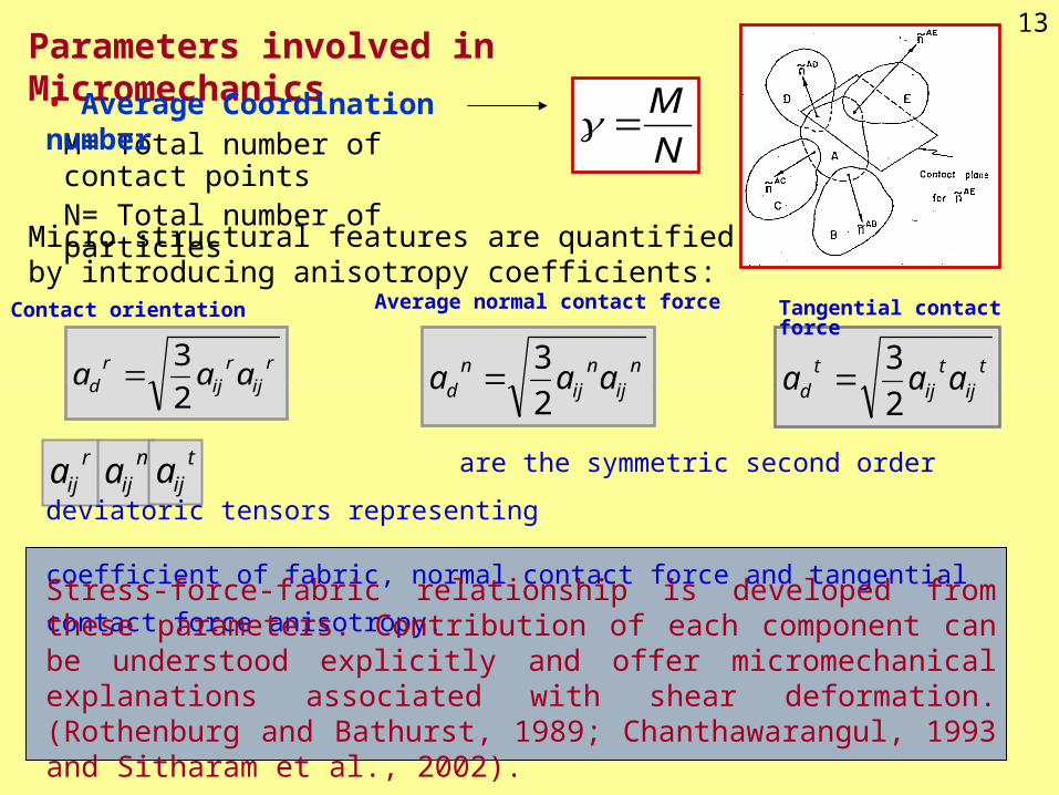
Parameters involved in Micromechanics

N

M

M= Total number of contact pointsN= Total number of particles

• Average Coordination number

rij

rij

rd aaa

2

3 n

ijn

ijn

d aaa2

3 t

ijt

ijt

d aaa2

3

Micro structural features are quantified by introducing anisotropy coefficients:

rija n

ija tija are the symmetric second order deviatoric tensors representing

coefficient of fabric, normal contact force and tangential contact force anisotropy.

Stress-force-fabric relationship is developed from these parameters. Contribution of each component can be understood explicitly and offer micromechanical explanations associated with shear deformation. (Rothenburg and Bathurst, 1989; Chanthawarangul, 1993 and Sitharam et al., 2002).

13

Tangential contact forceAverage normal contact forceContact orientation

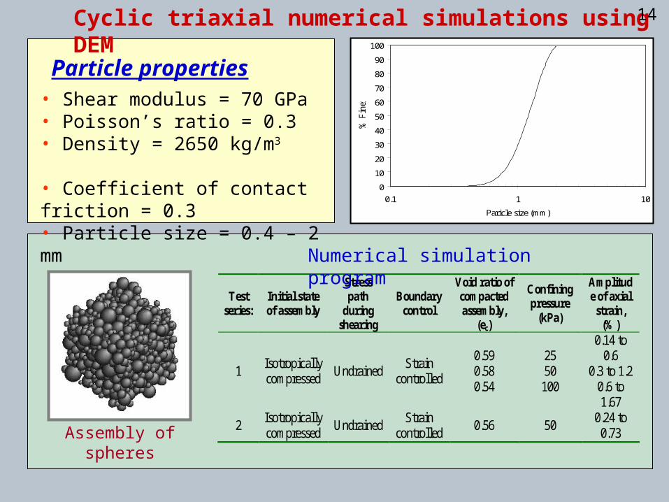
Cyclic triaxial numerical simulations using DEM

Test series:

Initial state of assembly

Stress path

during shearing

Boundary control

Void ratio of compacted assembly,

(ec)

Confining pressure

(kPa)

Amplitude of axial

strain, (%)

1 Isotropically compressed

Undrained Strain

controlled

0.59 0.58 0.54

25 50

100

0.14 to 0.6

0.3 to 1.2 0.6 to 1.67

2 Isotropically compressed

Undrained Strain

controlled 0.56 50

0.24 to 0.73

Numerical simulation program

• Shear modulus = 70 GPa• Poisson’s ratio = 0.3 • Density = 2650 kg/m3 • Coefficient of contact friction = 0.3 • Particle size = 0.4 – 2 mm

Particle properties

0

10

20

30

40

50

60

70

80

90

100

0.1 1 10

Paricle size (mm)

% F

iner

Assembly of spheres

14

-1

-0.8

-0.6

-0.4

-0.2

0

0.2

0.4

0.6

0.8

1

Number of cycles

Axi

al s

trai

n,

(%

)

1 2 3

3 = 50 kPa; ec = 0.58

= 0.6 %; f= 1.42 Hz

-20

-15

-10

-5

0

5

10

15

20

Number of cycles

Dev

iato

ric

stre

ss, q

(kP

a)

1 2 3

3 = 50 kPa; ec = 0.58

= 0.6 %; f= 1.42 Hz

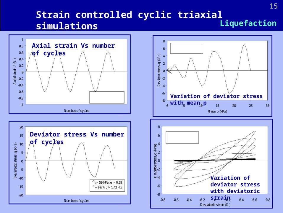
Strain controlled cyclic triaxial simulations

Axial strain Vs number of cycles

Deviator stress Vs number of cycles

-8

-6

-4

-2

0

2

4

6

8

0 5 10 15 20 25 30

Mean p (kPa)

Dev

iato

r st

ress

, q (

kPa)

3 = 25 kPa; ec = 0.59

f = 1.42 Hz

-8

-6

-4

-2

0

2

4

6

8

-0.8 -0.6 -0.4 -0.2 0 0.2 0.4 0.6 0.8Deviatoric strain (%)

Dev

iato

r str

ess,

q (k

Pa)

3 = 25 kPa; ec = 0.59

f = 1.42 Hz

Variation of deviator stress with deviatoric strain

Variation of deviator stress with mean p

Liquefaction

15

0

0.5

1

1.5

2

2.5

3

3.5

4

0 1 2 3 4 5 6 7

Number of cycles

Ave

rage

coo

rdin

atio

n nu

mbe

r

0

0.2

0.4

0.6

0.8

1

1.2

Pore

pre

ssur

e ra

tio, U

3 = 25 kPa; ec = 0.59

f = 1.42 Hz

Average coordination number

Pore pressure ratio

Plot of average coordination number and pore pressure ratio with number of cycles

0

0.5

1

1.5

2

2.5

3

3.5

4

-5 0 5 10 15 20 25

Mean p (kPa)

Ave

rage

coo

rdin

atio

n nu

mbe

r

3 = 25 kPa; ec = 0.59

f = 1.42 Hz

-40

-30

-20

-10

0

10

20

30

0 1 2 3 4 5 6 7

Number of cycles

Cha

nge

in n

umbe

r of c

onta

cts Vertical contacts

(80 -90

Horizontal contacts (0 -10

Average coordination Vs mean p

Change in the number of vertical and horizontal contacts Vs number of cycles

16

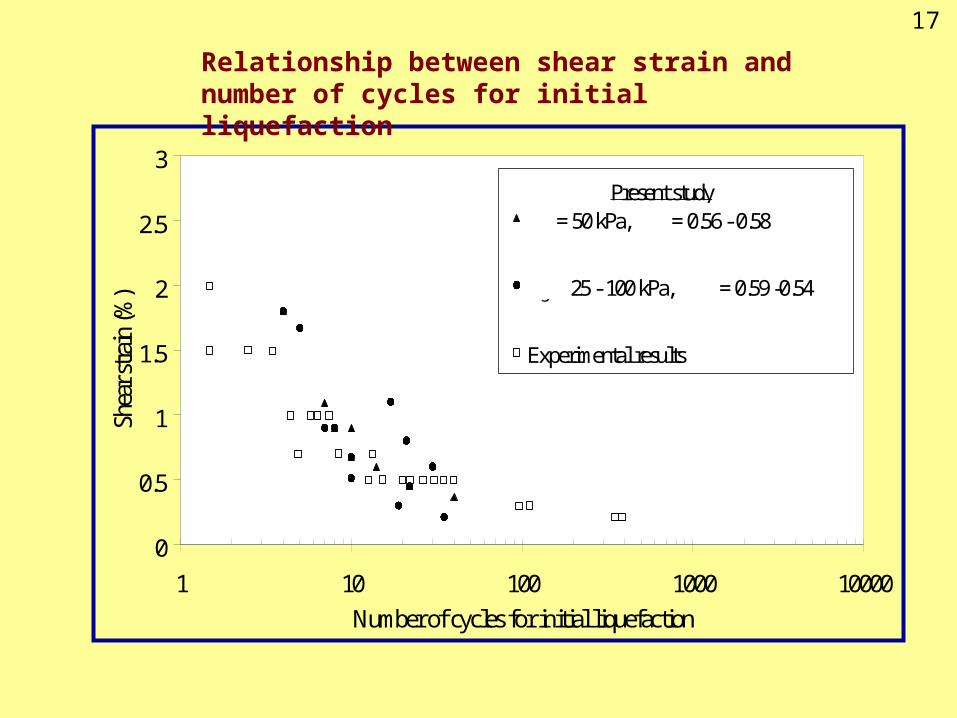
0

0.5

1

1.5

2

2.5

3

1 10 100 1000 10000

Number of cycles for initial liquefaction

Shea

r stra

in (%

)

= 50 kPa, = 0.56 - 0.58

25 - 100 kPa, = 0.59 -0.54

Experimental results

Talaganov (1996)

3 =

ec

Present study

3

ec

Relationship between shear strain and number of cycles for initial liquefaction

17

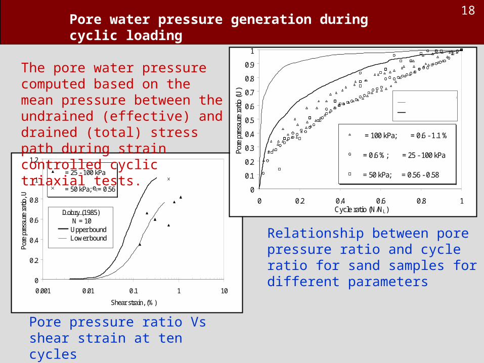
0

0.2

0.4

0.6

0.8

1

1.2

0.001 0.01 0.1 1 10

Shear strain, (%)

Pore

pre

ssur

e ra

tio, U

= 25 - 100 kPa

= 50 kPa; = 0.56

3

3

Dobry (1985) N = 10

Upper bound Lower bound

ec

0

0.1

0.2

0.3

0.4

0.5

0.6

0.7

0.8

0.9

1

0 0.2 0.4 0.6 0.8 1 Cycle ratio (N/NL)

Pore

pre

ssur

e ra

tio (

U)

= 100 kPa; = 0.6 - 1.1 %

= 0.6 %; = 25 - 100 kPa

= 50 kPa; = 0.56 - 0.58

3

3

3

ec

Talaganov (1996) Upper bound Lower bound

Pore water pressure generation during cyclic loading

The pore water pressure computed based on the mean pressure between the undrained (effective) and drained (total) stress path during strain controlled cyclic triaxial tests.

Relationship between pore pressure ratio and cycle ratio for sand samples for different parameters

Pore pressure ratio Vs shear strain at ten cycles

18

0

0.5

1

1.5

2

2.5

3

3.5

4

0 2 4 6 8 10 12Axial strain, (%)

Dev

iato

ric

anis

otro

pic

coef

fici

ent(

adn /a

dr /adt )

0

50

100

150

200

250

300

350

400

450

Dev

iato

r st

ress

, q (

kPa)

adn

adr

adt

3 = 100 kPa; ec = 0.54

= 0.6%

q

0

0.5

1

1.5

2

2.5

3

3.5

4

4.5

0 2 4 6 8 10 12Axial strain, (%)

Ave

rage

coo

rdin

atio

n nu

mbe

r

= 0.3 % 0.5 % 0.6 %

3 = 100 kPaec = 0.54

0

50

100

150

200

250

300

350

400

0 2 4 6 8 10 12Axial strain, (%)

Dev

iato

r st

ress

, q (

kPa)

= 0.3%

0.6 %

0.5%

3 = 100 kPa ec = 0.54

0

50

100

150

200

250

300

350

400

0 100 200 300 400 500Mean p (kPa)

Dev

iato

r st

ress

, q (

kPa)

3 = 100 kPaec =0.54

Post liquefaction behaviour of granular materials

Deviator stress Vs

mean p

Deviator anisotropic coefficients and deviator stress Vs axial strain

Deviator stress Vs

axial strain

Average coordinaion number Vs

axial strain

19

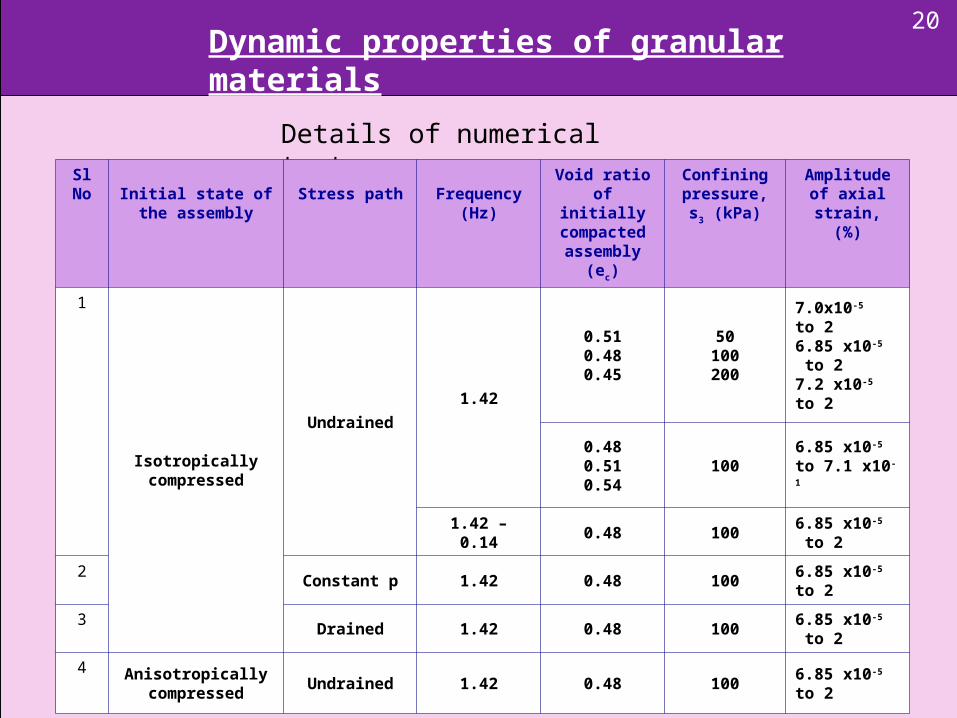
Dynamic properties of granular materials

Details of numerical test program

Sl No Initial state of the

assemblyStress path Frequency

(Hz)

Void ratio of initially

compacted assembly (ec)

Confining pressure, s3

(kPa)

Amplitude of axial strain,

(%)

1

Isotropically compressed

Undrained1.42

0.510.480.45

50100200

7.0x10-5

to 26.85 x10-5 to 27.2 x10-5

to 2

0.480.510.54

1006.85 x10-5 to 7.1 x10-1

1.42 – 0.14 0.48 100 6.85 x10-5 to 2

2 Constant p 1.42 0.48 100 6.85 x10-5 to 2

3 Drained 1.42 0.48 100 6.85 x10-5 to 2

4 Anisotropicallycompressed

Undrained 1.42 0.48 100 6.85 x10-5 to 2

20

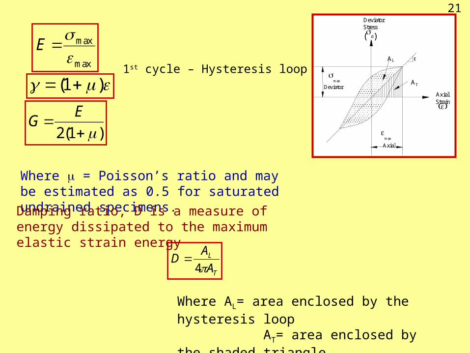
AxialStrain

DeviatorStress

(d)

AT

AL E

max

Axial

max

Deviator

max

max

E

)1(

)1(2

EG

T

L

A

AD

4

Where = Poisson’s ratio and may be estimated as 0.5 for saturated undrained specimens.

Damping ratio, D is a measure of energy dissipated to the maximum elastic strain energy

Where AL= area enclosed by the hysteresis loop AT= area enclosed by the shaded triangle

1st cycle – Hysteresis loop

21

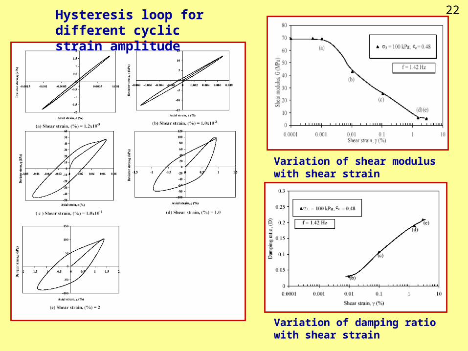
Hysteresis loop for different cyclic strain amplitude

Variation of shear modulus with shear strain

Variation of damping ratio with shear strain

22

0

0.05

0.1

0.15

0.2

0.25

0.3

0.0001 0.001 0.01 0.1 1 10

Shear strain, (%)

Dam

ping

ratio

, (D

)

= 50 kPa; = 0.51

= 100 kPa; = 0.48

= 200 kPa = 0.45

3

3

3

ec

ec

ec

f = 1.42 Hz

Seed and Idriss (1970) Upper bound Lower bound

0

0.1

0.2

0.3

0.4

0.5

0.6

0.7

0.8

0.9

1

0.0001 0.001 0.01 0.1 1 10Shear strain, (%)

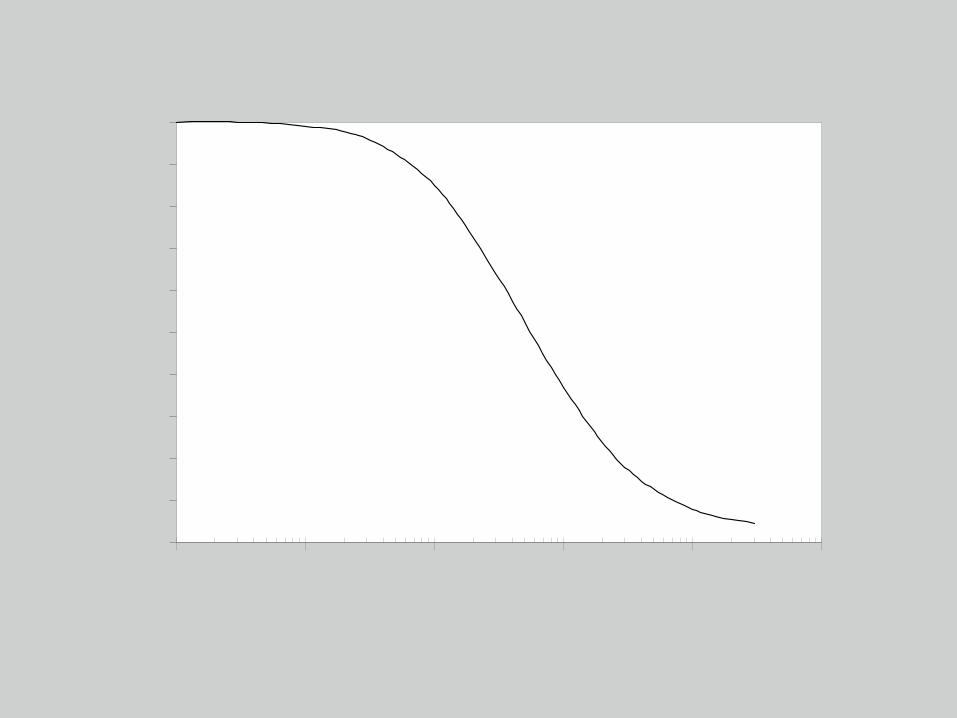
Mod

ulus

ratio

(G/G

0)

= 0.48

= 0.51

= 0.54

Seed and Idriss, (1970) Upper bound Lower bound

3 = 100 kPaf = 1.42 Hz

ec

ec

ec

0

0.1

0.2

0.3

0.4

0.5

0.6

0.7

0.8

0.9

1

0.0001 0.001 0.01 0.1 1 10Shear strain, (%)

Mod

ulus

rat

io (

G/G

0)

= 50 kPa; = 0.51

= 100 kPa; = 0.48

= 200 kPa; = 0.45


3

f = 1.42 Hz

3

3

ec

ec

ec

0

0.05

0.1

0.15

0.2

0.25

0.3

0.0001 0.001 0.01 0.1 1 10Shear strain, (%)

Dam

ping

ratio

(D)

= 0.48 = 0.51 = 0.54


3 = 100 kPaf = 1.42 Hz

ec

ecec

Effect of confining pressure Effect of void ratio

Modulus ratio vs shear strain

Modulus ratio Vs shear strain

Damping ratio Vs shear strain


23

0

10

20

30

40

50

60

70

80

90

100

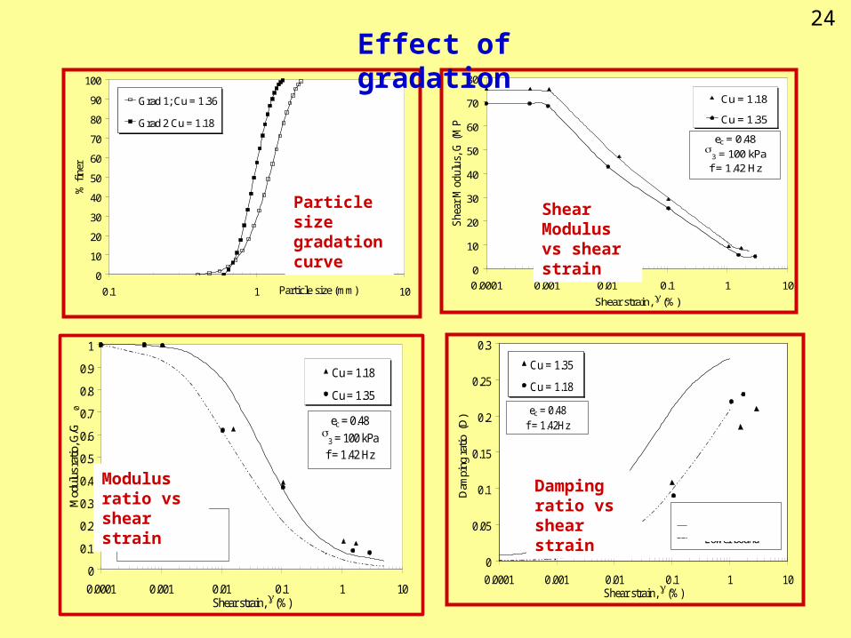
0.1 1 10Particle size (mm)

% f

iner

Grad 1; Cu = 1.36

Grad 2 Cu = 1.18

0

0.05

0.1

0.15

0.2

0.25

0.3

0.0001 0.001 0.01 0.1 1 10Shear strain, (%)

Dam

ping

ratio

(D

)

Cu = 1.35

Cu = 1.18

Seed and Idriss(1970) Upper bound Lower bound

ec = 0.48 f = 1.42Hz

Particle size gradation curve

0

10

20

30

40

50

60

70

80

0.0001 0.001 0.01 0.1 1 10

Shear strain, (%)

She

ar M

odul

us, G

(M

Pa)

Cu = 1.18

Cu = 1.35

ec = 0.48

3 = 100 kPaf = 1.42 Hz

0

0.1

0.2

0.3

0.4

0.5

0.6

0.7

0.8

0.9

1

0.0001 0.001 0.01 0.1 1 10Shear strain, (%)

Mod

ulus

ratio

, G/G

0

Cu = 1.18

Cu = 1.35


ec = 0.48

3 = 100 kPaf = 1.42 Hz

Effect of gradation

Shear Modulus vs shear strain

Damping ratio vs shear strain

Modulus ratio vs shear strain

24

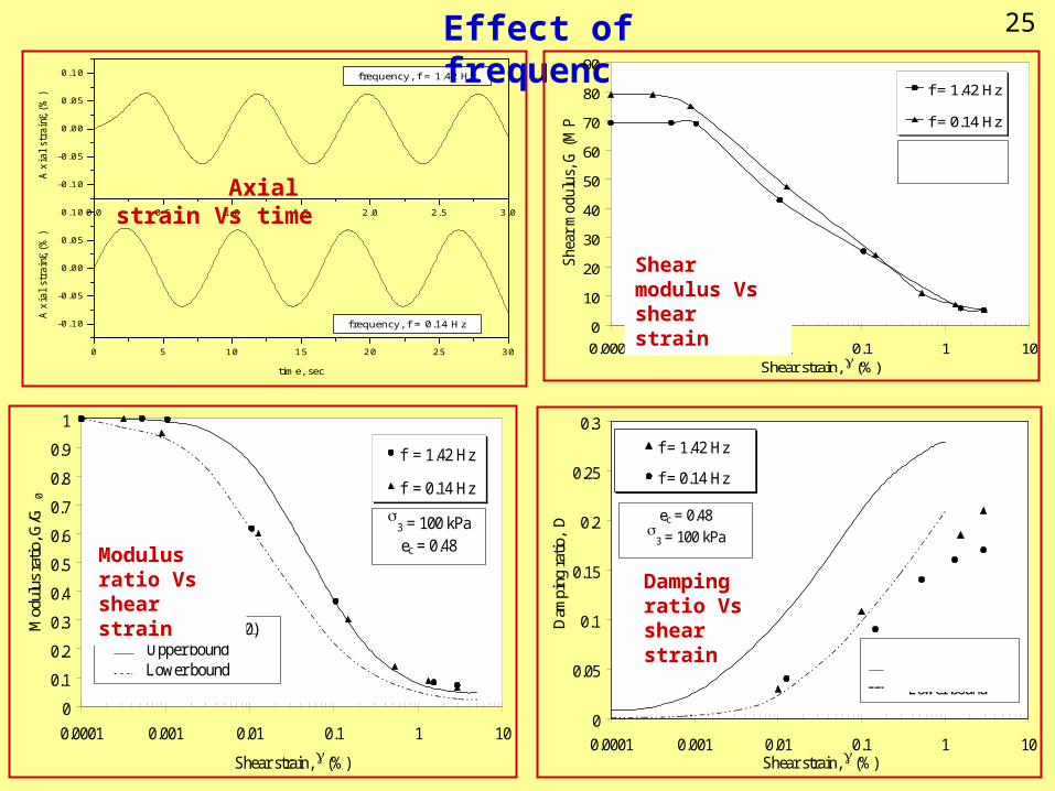
0 5 10 15 20 25 30

-0.10

-0.05

0.00

0.05

0.10 0.0 0.5 1.0 1.5 2.0 2.5 3.0

-0.10

-0.05

0.00

0.05

0.10

Axia

l st

rain

, (%

)

time, sec

frequency, f = 0.14 Hz

A

xia

l st

rain

, (%

)

frequency, f = 1.42 Hz

Effect of frequency

0

10

20

30

40

50

60

70

80

90

0.0001 0.001 0.01 0.1 1 10Shear strain, (%)

Sh

ear

mo

du

lus,

G (

MP

a)

f = 1.42 Hz

f = 0.14 Hz

3 = 100 kPaec = 0.48

0

0.1

0.2

0.3

0.4

0.5

0.6

0.7

0.8

0.9

1

0.0001 0.001 0.01 0.1 1 10

Shear strain, (%)

Mod

ulus

ratio

, G/G

0

f = 1.42 Hz

f = 0.14 Hz

3 = 100 kPaec = 0.48

Seed and Idriss (1970)Upper boundLower bound

0

0.05

0.1

0.15

0.2

0.25

0.3

0.0001 0.001 0.01 0.1 1 10Shear strain, (%)

Dam

ping

rat

io,

D

f = 1.42 Hz

f = 0.14 Hz


ec = 0.48

3 = 100 kPa

Shear modulus Vs shear strain

Axial strain Vs time

Modulus ratio Vs shear strain Damping ratio

Vs shear strain

25

0

20

40

60

80

100

120

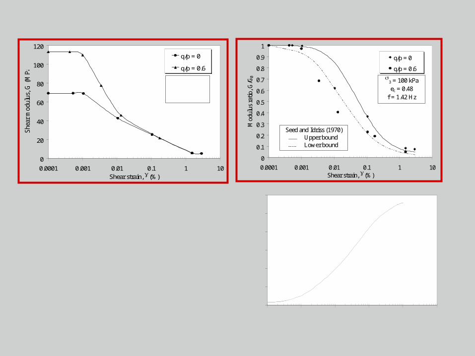
0.0001 0.001 0.01 0.1 1 10Shear strain, (%)

She

ar m

odul

us, G

(M

Pa)

q/p = 0

q/p = 0.6

3 = 100 kPaec = 0.48

f =1.42 Hz

0

0.1

0.2

0.3

0.4

0.5

0.6

0.7

0.8

0.9

1

0.0001 0.001 0.01 0.1 1 10Shear strain, (%)

Mod

ulus

rat

io, G

/G0

q/p = 0

q/p = 0.6

3 = 100 kPaec = 0.48

f = 1.42 Hz


0

0.05

0.1

0.15

0.2

0.25

0.3

0.0001 0.001 0.01 0.1 1 10

Shear strain, (%)

Dam

ping

rat

io (

D)

q/p = 0

q/p = 0.6

3 = 100 kPaec = 0.48

f = 1.42 Hz


Effect of Initial Anisotropy




26

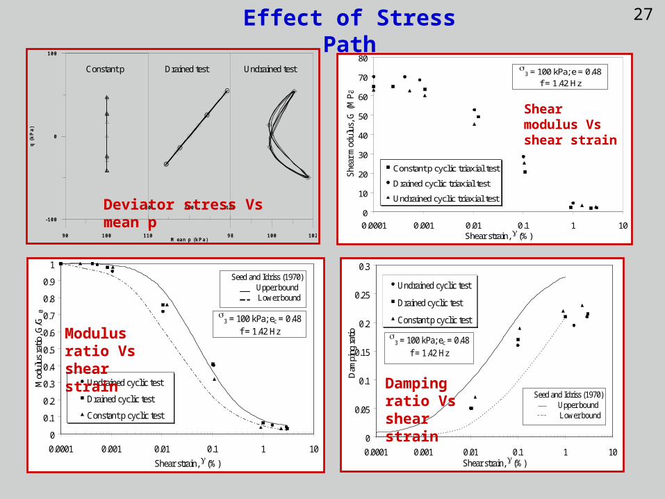
Constant p Drained test Undrained test

90 1 00 110

-100

0

1 00

q (

kPa)

8 0 100 12 0

M ean p (k P a )9 8 100 10 2

0

10

20

30

40

50

60

70

80

0.0001 0.001 0.01 0.1 1 10Shear strain, (%)

She

ar m

odul

us, G

(M

Pa)

Constant p cyclic triaxial test

Drained cyclic triaxial test

Undrained cyclic triaxial test

3 = 100 kPa; e = 0.48

f = 1.42 Hz

0

0.1

0.2

0.3

0.4

0.5

0.6

0.7

0.8

0.9

1

0.0001 0.001 0.01 0.1 1 10

Shear strain, (%)

Mod

ulus

ratio

, G/G

0

Undrained cyclic test

Drained cyclic test

Constant p cyclic test

Seed and Idriss (1970) Upper bound

Lower bound

3 = 100 kPa; ec = 0.48

f = 1.42 Hz

0

0.05

0.1

0.15

0.2

0.25

0.3

0.0001 0.001 0.01 0.1 1 10Shear strain, (%)

Dam

ping

ratio

Undrained cyclic test

Drained cyclic test

Constant p cyclic test

Seed and Idriss (1970) Upper bound

Lower bound

3 = 100 kPa; ec = 0.48

f = 1.42 Hz

Effect of Stress Path



Deviator stress Vs mean p


27

0

0.1

0.2

0.3

0.4

0.5

0.6

0.7

0.8

0.9

1

0.0001 0.001 0.01 0.1 1 10

Shear strain, (%)

Mod

ulus

ratio

, G/G

0

= 50 - 100 kPa; = 0.51 -0.45

= 100 kPa; = 0.48 - 0.54

= 100 kPa; = 0.48; cu = 1.18 - 1.35

= 100 kPa; = 0.48; f = 0.42 - 1.42

= 100 kPa; = 0.48; q/p = 0 - 0.6

Constant p cyclic triaxial test 3 = 100 kPa; ec = 0.48; f = 1.42 Hz

Drained cyclic triaxial test

3 = 100 kPa; ec = 0.48; f = 1.42 Hz


Undrained cyclic triaxial test

3

3

3

3

3

ec

ec

ec

ec

ec


28

0

0.05

0.1

0.15

0.2

0.25

0.3

0.0001 0.001 0.01 0.1 1 10Shear strain, (%)

Dam

ping

rat

io, (

D)

= 50 - 100 kPa; = 0.51 - 0.45

= 100 kPa; = 0.48 -0.54

= 100 kPa; = 0.48; Cu = 1.18 -1.35

= 100 kPa; = 0.48; f = 0.42 - 1.42 Hz

= 100 kPa; = 0.48; q/p = 0 - 0.6

Constant p cyclic triaxial test 3 = 100 kPa; ec = 0.48; f = 1.42 Hz

Drained cyclic triaxial test 3 = 100 kPa; ec = 0.48; f = 1.42 Hz

3

3

3

3

ec

ec

ec


3

ec

Undrained cyclic triaxial testec


29

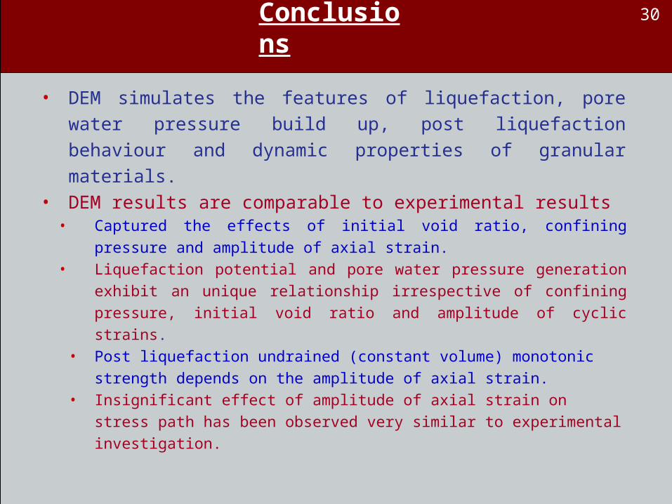
Conclusions

• DEM simulates the features of liquefaction, pore water

pressure build up, post liquefaction behaviour and dynamic

properties of granular materials. • DEM results are comparable to experimental results

• Captured the effects of initial void ratio, confining pressure and

amplitude of axial strain. • Liquefaction potential and pore water pressure generation exhibit an

unique relationship irrespective of confining pressure, initial void

ratio and amplitude of cyclic strains. • Post liquefaction undrained (constant volume) monotonic strength

depends on the amplitude of axial strain. • Insignificant effect of amplitude of axial strain on stress path has

been observed very similar to experimental investigation.

30

Liquefaction IIT Roorkee Dec 26 2012

Documents

Transcript of Liquefaction IIT Roorkee Dec 26 2012