Linking Users Across Domains with Location Data:Theory and Validation

Chris Riederer, Yunsung Kim,Augustin Chaintreau

Columbia UniversityNew York, NY

{mani,augustin}@cs.columbia.eduyunsung.kim@columbia.edu

Nitish Korula, Silvio LattanziGoogle Research

New York, NY{nitish,silviol}@google.com

ABSTRACTLinking accounts of the same user across datasets – evenwhen personally identifying information is removed or un-available – is an important open problem studied in manycontexts. Beyond many practical applications, (such as crossdomain analysis, recommendation, and link prediction), un-derstanding this problem more generally informs us on theprivacy implications of data disclosure. Previous work hastypically addressed this question using either different por-tions of the same dataset or observing the same behavioracross thematically similar domains. In contrast, the generalcross-domain case where users have different profiles inde-pendently generated from a common but unknown patternraises new challenges, including difficulties in validation, andremains under-explored.

In this paper, we address the reconciliation problem forlocation-based datasets and introduce a robust method forthis general setting. Location datasets are a particularlyfruitful domain to study: such records are frequently pro-duced by users in an increasing number of applications andare highly sensitive, especially when linked to other data-sets. Our main contribution is a generic and self-tunablealgorithm that leverages any pair of sporadic location-baseddatasets to determine the most likely matching between theusers it contains. While making very general assumptionson the patterns of mobile users, we show that the maximumweight matching we compute is provably correct. Althoughtrue cross-domain datasets are a rarity, our experimentalevaluation uses two entirely new data collections, includingone we crawled, on an unprecedented scale. The method wedesign outperforms naive rules and prior heuristics. As itcombines both sparse and dense properties of location-baseddata and accounts for probabilistic dynamics of observation,it can be shown to be robust even when data gets sparse.

Copyright is held by the International World Wide Web Conference Com-mittee (IW3C2). IW3C2 reserves the right to provide a hyperlink to theauthor’s site if the Material is used in electronic media.WWW 2016, April 11–15, 2016, Montréal, Québec, Canada.ACM 978-1-4503-4143-1/16/04.http://dx.doi.org/10.1145/2872427.2883002 .

1. INTRODUCTIONAlmost every interaction with technology creates digital

traces, from the cell tower used to route mobile calls to thevendor recording a credit card transaction; from the pho-tographs we take, to the “status updates” we post online.The idea that these traces can all be merged and connectedis both fascinating and unsettling. The ability to merge dif-ferent datasets across domains can provide individuals withenormous benefits, as seen by increasingly widespread adop-tion of apps that learn multi-domain user behavior and pro-vide helpful recommendations and suggestions. However,when done by third parties that a user may not interactwith directly, this raises fundamental questions about dataprivacy. In this paper, we focus on location data and showthat this type of data is privacy sensitive. More formally,we focus on the following technical question: Is it possibleto link accounts of the same user across datasets using justlocation data? The answer to that question points bothto algorithmic feasibility but also our ability to maintainseemingly distinct identities or personas until one choosesto reveal they belong to the same user.

Increasingly often, as shown in recent studies, the loca-tion of a smartphone owner is captured and recorded for amajority of mobile apps even in the absence of geographi-cal personalization. This considerably expands the numberof parties who can collect and exploit the knowledge of auser’s whereabouts. Even when data is recorded sporadi-cally, these datasets are very rich and intimately connectedto one’s everyday life; they may present or at least par-tially reflect our most recognizable patterns. Recently, evena small amount of location information was shown sufficientto either render most users distinguishable [7, 25], or infermultiple sociological traits such as race [18], friendship [4,6], gender, or marital status when combined with domainsemantic information [27].

In spite of this work, determining when and how two ac-counts belong to the same mobile user in different domainsremains an open problem, primarily for three reasons: First,identity reconciliation is harder than both classifying anddistinguishing users. As an example of the former, one maynot be able to connect two profiles exactly, but can still bequite certain that both belong to a high-income American,for instance. For the latter, uniqueness of an individual inone dataset does not imply that they will be easily recog-nized in another one. For instance, in a simple case whereindividuals produce location records randomly and indepen-dently in two domains, users will likely be unique but it is

provably impossible to link them across datasets. Second, asa consequence, many previous methods are domain specificand typically focus on clean and dense parts of the data. Incontrast, most of our motivating examples above are sparse,and we aim at leveraging locations in the general case with-out additional information attached. Third, with almost noexceptions, identity reconciliation was always considered fordifferent parts of the exact same data set, or at best do-mains that are semantically similar. In contrast, our goalis to address the most general case in which records acrossdomains are separately generated but share an underlyingpattern: The user’s physical location. Since one cannot oc-cupy two locations at the same time, the common pattern ofour physical mobility creates fertile ground to notice eventsthat coincide, and those that are incompatible. The mainquestion is how to use those observations (ideally in a prov-ably optimal manner), under which conditions they are suffi-cient to link accounts, and how to collect data to empiricallyvalidate any related claims.

Exploiting rare coincidences to de-anonymize users is nowa classic problem, with a sparsity based method availablefor almost a decade [15]. While we defer a more detailedcomparison with our work to the next section, we wouldlike to point out the main ingredient of our algorithm: anew use of misses and repetitions to interpret coinciden-tal records that exploits the sparse property of coupling be-tween Poisson processes. We note that sporadic collectionof records typically resembles such statistics for rare events.This method, which is proved optimal and correct underthese simple assumptions, is hence particularly effective invarious datasets. Another advantage of our scheme is that itrelies on only three parameters1 that are initially unknownbut easy to approximate. We prove empirically that simplemethods to estimate these parameters are robust even whenstarting from imperfect observations.

We now present the following contributions.

• A new generic and self-tunable algorithm which com-bines positive and negative signals from co-incidentevents to build a new type of maximum weight match-ing. In practice this algorithm is compatible with a pa-rameter tuning step exploiting a previously proposeddensity-based method. In spite of no domain-specifictuning, our algorithm outperforms the state of the art.

• A rigorous interpretation of our algorithm justifying itscorrectness. In particular we provide a simple modelof mobility that encompasses various cases of location-based data. This is, to the best of our knowledge, thefirst mathematical model for observed location tracesacross multiple domains. We prove the ideal correctmatching maximizes our algorithm’s score and con-versely, that only correct matching achieves maximumscore in expectation.

• An empirical evaluation of this problem in three dis-tinct scenarios that significantly extends beyond pre-vious studies in both realism and scope. The firstdataset, already publicly available, allows immediatecomparison with prior results. For the second scenarioconsidered, we collected data from two current live ser-vices, gathering considerably more locations, and prov-ing that our method achieves near perfect accuracy.

1Two are related, so estimation has two degrees of freedom.

Finally, our method is shown superior in a commercialscenario that is significantly more heterogeneous andchallenging2.

As we explained above, linking anonymous profiles acrossdomains is considerably more challenging than either estab-lishing users’ distinguishability or classifying users into dif-ferent groups. As such, it may have been considered imprac-tical at scale. The fact that we can link users, sometimeswith high precision and recall, shines new light on the pro-tection offered by even the most complete anonymity. Ourresults are, to the best of our knowledge, the first exampleof a cross domain analysis of this problem to prove an al-gorithm’s correctness, together with the first validation atscale of location based reconciliation in real cases. As moredata are available, and different patterns or domain specificproperties are discovered, we believe that more algorithmscould be designed and evaluated against the technique wepresent as a benchmark for the most general case.

2. RELATED WORKIt has been shown that most users in location based da-

tasets are unique, either through a few of their most visitedplaces [25] or based on a few timed visits chosen at ran-dom [7, 8]. This property follows a tradition of work spec-ifying the risk of releasing even anonymized datasets [21].What this shows is that users can be re-identified in theory,for instance in one of the following two cases: if an adversaryhas access to auxiliary information (e.g., the real identity ofall users who visited a place at a given time, or an orig-inal set of seed nodes which are already re-identified) [7],or alternatively if a public data set is known to intersectthe anonymized one [21]. What those works do not show,however, is how to exploit this uniqueness in the commoncase we consider: two distinct datasets with no auxiliaryinformation that is known a priori.

Identity reconciliation so far has leveraged three princi-ples: Ad-hoc identifying features such as matching username,email addresses, or unique tags. Those are ignored here;as recently measured in [10] they are rarely available andaccurate. Information propagation, where starting from aseed set of identified nodes, a graphical structure such asa social network is exploited to expand the set of matchednodes in static [12, 13, 16, 17, 24] or mobile [20, 11] data-sets. Again, those techniques cannot be applied in the gen-eral case where no preexisting graph and seeds are known3.Finally, identification of nearest neighbors using similaritymetrics [15, 9] generalizes the first method to leverage non-identifying features and imperfect matches. Data sparsityplays an important role, which is typically included in thedesign of the similarity metric. This approach suffers fromthe opposite problem: it applies so broadly that it is very

2This dataset was not released in raw form to any researcherin the team; the evaluation was run on a remote server witha non-exclusive agreement that other academic researcherscan replicate in the spirit of reproducing and improving fu-ture reconciliation methods. Note that the authors fromGoogle did not have even remote access to this data.3In the most ambitious information propagation where seedsmay be noisy and structures, initially unknown, are inferred,the differences between this approach and one based on sim-ilarity starts to fade. We experimented with it but found noimprovement from information propagation to report.

loosely defined. Indeed, most successful reconciliations us-ing this technique report on the art of deciding upon in-formative similarity features – or often the subtlety of theircombined effects [9] – without necessarily providing a unifiedjustification. Moreover, a closer look showed that the accu-racy of similarity methods for static features (e.g., name,home location, friends) are typically overestimated in prac-tice [10]. Our work addresses this important need: Ourinference method interprets location datasets, however dif-ferent in their domains, as sporadic observations of the samehidden mobility processes. We generalize data sparsity froma static viewpoint to a dynamic viewpoint, leveraging nat-urally misses and repetitions in the observed processes. Inspite of a considerable amount of prior work on Entity Res-olution [5], we did not find similar analysis and algorithms,probably because mobile datasets are relatively new and ex-hibit specific dynamics. Similarly, the related literature onnetwork alignment [1] rarely considers the bipartite case [14]and it centers on static graphs. We empirically found thatour method yields superior accuracy to those previously pro-posed, while being more robust and easy to use.

Other attempts at re-identifying users using mobility dataonly have typically expressed similarity between users withdensity based methods [23, 9]. Those rely on a user havinga discriminative pattern in the frequency she visits variousplaces. In [23] author aims at reconciling users in the samedomain but at different periods, hence ignoring the time ofthe visits themselves. In situations where datasets overlapin time, those techniques leave much information unused.4

Another technique, somewhat diametrically opposed, usesspecific visit times [19]. Prior to this paper, this was onlyvalidated in a single domain (by randomly extracting a sub-set of each user’s profile to recognize). We empirically showthat none of those methods extend to the more demandingcross domain case without incurring large inaccuracy. Thisconfirms previous observations that density and time basedsimilarities can reduce the scope of re-identification attacksby removing a lot of dissimilar accounts [9], but cannot beused as is for reconciliation as they lead to low accuracyin practice [10]. Finally, we should mention a statisticallearning approach based on Dirichlet distribution used torelate anonymous CDR data with publicly available socialnetwork data [2, 3]. It remains, however, difficult to judgeits effectiveness as it is used without further theoretical jus-tification and validated without ground truth in the data.Our method, in contrast, is tailored from scratch to locationbased datasets, its correctness is proved under simple as-sumption on nodes’ visits, and it has been evaluated on threedata-sets with ground truth, among the largest available todate, including two that have never appeared in this con-text. Whether more generic statistical learning reproducessome of the strength of our method remains an interestingquestion to explore beyond the scope of this paper.

3. LOCATION-BASED RECONCILIATION

3.1 Problem Formulation and ModelWe use U and V to denote the set of n user accounts in

the two domains, with accounts to be linked using location-

4It is, for instance, entirely ineffective in a homogeneouspopulation where each user follows the same location distri-bution for her visits. Our method, in contrast, is proved tocorrectly handle that case.

based data. Let σI denote the true (“identity”) mappingthat correctly links the two accounts of the each user. Theusers may visit locations at various times and perform anaction (such as a checkin), which results in the creation of arecord in one of the datasets. Each such record is associatedwith the location and time-stamp, and possibly additionalsemantic information that is relevant to this dataset, butmay not make sense in a different domain. Therefore, inour algorithm, we only use the time-stamped location data.Note that locations and times may be recorded at a differ-ent granularity and levels of precision in the two differentdatasets to be reconciled (for instance, one may only recordthe nearest cell tower, the other has GPS coordinates). Toaccount for this, we divide locations and times into bins,corresponding to a geographical region or interval of time;For a fixed bin corresponding to location region ` and timeinterval t, any action recorded in region ` during time inter-val t is associated with bin (`, t). We use L to denote theset of all location regions and T the set of time intervals inthe union of our datasets.

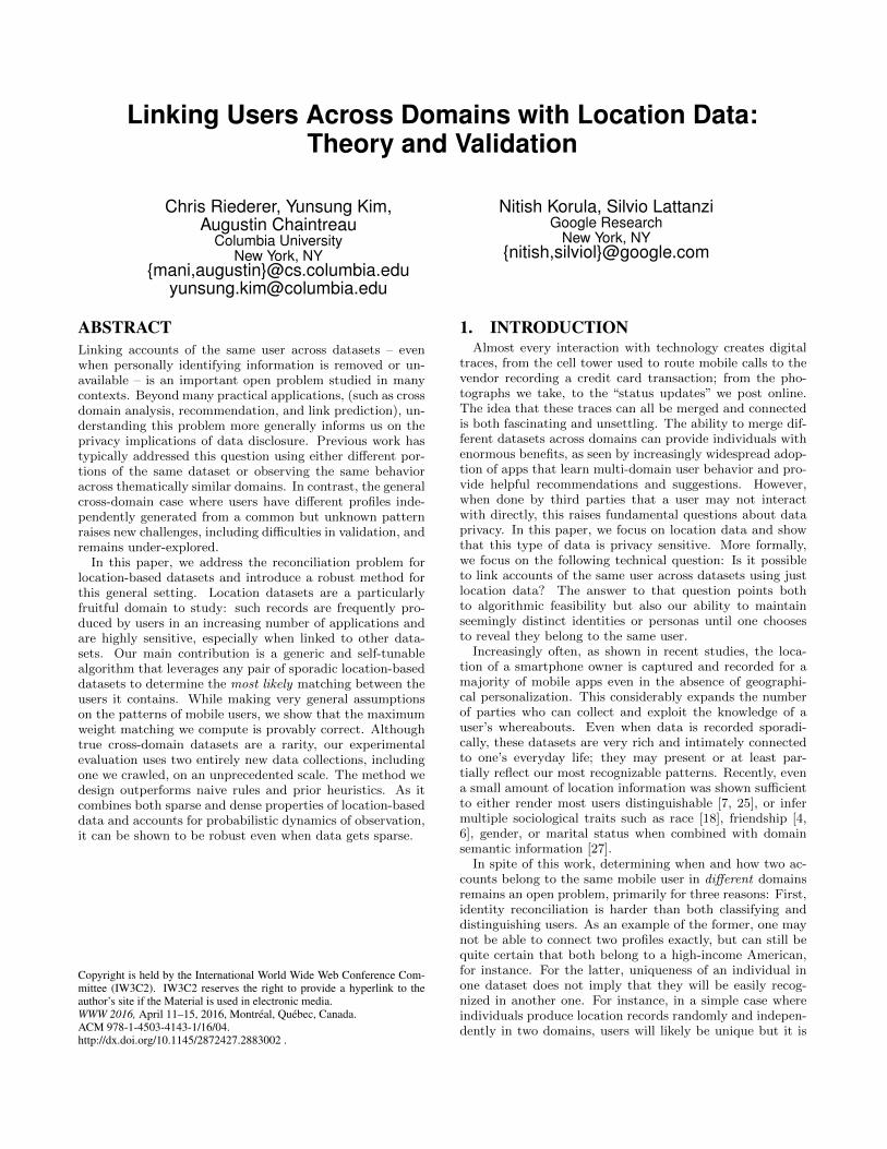
As shown in Figure 1, although each user u or v physicallyfollows a continuous time trajectory Mt (shown on the left),her mobility record r(u) in each domain is defined as themulti-set of (location, time) bins in which she took an ac-tion: r(u) = {(`1, t1), (`2, t2), . . . }. Note that it is importantthat this is a multiset: if a user records 2 actions in the samebin, this bin is present twice in the mobility record. Given aspecific (location, time) pair (`, t) we denote the number ofactions in domain 1 that user u took by a1(u, `, t) (i.e., thenumber of occurrences of (`, t) in the multiset r1(u)). Wedefine a2(u, `, t) similarly for domain 2. For ease of nota-tion, we use a1 (respectively a2) to denote a1(u, `, t) (resp.a2(u, `, t)) when u, `, t are clear from the context.

In this paper, we focus on reconciling users across twodomains based only on their mobility records, which werefer to as r1(u) and r2(u) respectively. In other words,given a collection of mobility records

{r1(u)

∣∣ u ∈ U }and{

r2(u)∣∣ u ∈ V }

for the same population but with no iden-tity attached, our goal is to return the true mapping σIwhich maps the record belonging to one user to the recordof the same user in the other collection.

3.2 Mobility Model and AssumptionsIn order to formally analyze algorithms applying to the

cross-domain reconciliation problem defined above, it is nec-essary to work under a given mobility model which governshow users produce records. Without such assumption, onlyworst-case performance can be measured, which is arbitrar-ily bad for any algorithm since one can devise instanceswhere the set of locations with actions in domain 1 is com-pletely disjoint from the set of locations with actions in do-main 2. Providing the first such model and proving it leadsto a practical method is one of our key contributions.

We assume the mobility records follow a simple generationprocess: First, for each (location, time) pair, the number ofvisits of each user to this location during this time periodfollows a Poisson distribution, with rate parameter λ`,t andthis choice is independent of the visits produced for anyother pair. It is a rather crude but effective assumption,as it combines mathematical simplicity (critical later to jus-tify our method), and a form of robustness. Indeed, Poissondistributions are known to be good approximations of rareevent processes and to combine gracefully when summed, al-

time tMt(u)

l5,t51

cell number1 2 3 4 5 6 7space

using 1 time-bin

Records

1

l4,t41 1

l3,t31 1

l2,t21 1

l1,t11 1

l3,t32 2

l2,t22 2

l1,t12 2

r (u)1 r (u)2

Domain 1

1 2 3 4 5 6 7

1 2 3 4 5 6 7

1 2 3 4 5 6 7

using 2 time-bins

using 4 time-bins

Domain 2

Trajectory Multi-set t

l

r (v)1 r (v)2

l2,t22 2

l1,t22 2

l2,t22 2

l1,t22 2

Mt(v)

Figure 1: Two space-time trajectories with associated footprints in two domains.

lowing multiple granularity levels to be combined. They arequite commonly used to handle robust parameter estima-tion, which is important as the parameter λ`,t is unknownto the algorithm.

The characterization above describes how visits are pro-duced, but does not specify how users perform actions thatare observed. We assume that each time the user visits alocation, an action in domain 1 and domain 2 occurs, in-dependently of each other, with probabilities p1 and p2 re-spectively. Thus, the mobility records are random variables,which we denote by R1(u) and R2(u) respectively, with thenumber of actions in a given bin (`, t) being random vari-ables denoted by A1(u, `, t) and A2(u, `, t) respectively. Theprocess of visits and action in each domain is also assumedto be independent among users.

Possible extensions: While we keep the model to itssimplest form for the sake of a clear exposition, the argu-ments we provide in this paper generalize to multiple othercases. First among them, all results apply as well when theprobability p1 and p2 could depend on l and t as well. Onecould also analyze our algorithms when those parametersare not constant among users. After experimenting withthose more general models, we found that they do not yieldsignificant practical improvement in the scenarios we evalu-ated. We also note that one can adopt different generativemodels, but many of these do not change the problem signif-icantly, or the analysis of our algorithm. For instance, thenumber of visits to a particular location may be generatedby a binomial distribution, instead of Poisson.

Other extensions are interesting topics for further study:For example, our model does not currently account for ge-ographical proximity between different locations; in reality,users who visit a location ` are also likely to visit a nearbylocation `′. One advantage is that this keeps our modelgeneral and robust to variations in formats and resolutionacross datasets that are quite common in space-time data.For instance, actions 1km apart may be considered close ina rural setting but far in an urban area. Our method is ag-nostic to such relative change of distance. We also note thatour model ignore dependencies between users. For instance,members of a family may travel together and the presenceof friends in a location may render a visit by a given personmore likely. On the other hand, our model can accommo-

date frequency of visits that vary between users and hencecreate communities that on average visit frequently similarplaces. With larger and richer data, it is likely that morerealistic models than ours may give additional insights andbetter exploit users’ true mobility patterns. However, thesimple case we define above leads to a simple algorithm thatcaptures mobility of users sufficiently well to beat the stateof the art and present a reasonable benchmark for futureuse.

4. ALGORITHM AND ANALYSISIn this Section, we present an algorithm tailored to the

location record model introduced above. Our main contri-bution is a proof that under these assumptions, there is atight correspondence between the maximum weight match-ing that we define and the ‘true’ matching between users,even exhibiting a positive gap. Later, Section 5 will demon-strate that this correspondence generalizes in practice tomake this algorithm a superior alternative to multiple knownapproaches.

4.1 AlgorithmOur algorithm works in two phases: The first phase is to

compute a score for every candidate pair of users (u, v) ∈U × V (see below for more details). In a second phase,we first define a complete bipartite graph on (U, V ) wherethe weight of the edge (u, v) is given by the score for (u, v)aforementioned. We then compute the matching in this bi-partite graph that has maximum weight5. The algorithmthen claims that records that are connected by an edge be-long to the same user. Under the assumptions introducedabove, we can prove that this procedure is always correct.

In the rest of this section, we provide more details onhow the scores of a pair (u, v) are determined: For each(location, time) bin (`, t), we compute Score(u, v, `, t) =ln (φ`,t(a1, a2)), where the term φ`,t in the logarithm is:

P [A1(u, `, t) = a1 ∧A2(v, `, t) = a2 | σI(u) = v]

P [A1(u, `, t) = a1] · P [A2(v, `, t) = a2].

5If some edges have negative weight it is possible in the-ory for a maximum weight matching not to match all users.However, under our assumptions it does not happen.

The numerator of φ measures the probability that the sameuser performs a1 actions in domain 1 and a2 actions in do-main 2 in the bin (`, t). The two terms in the denominatorare the probability that an arbitrary user performs a1 ac-tions in domain 1 in bin (`, t), and another user performsa2 actions in domain 2 in this bin. Since we assume thatuser performs actions independently, φ`,t(a1, a2) measureshow much more likely it is to observe a1 actions in domain1 by account u and a2 actions in domain 2 by account v ifthese accounts belong to the same user than if these are twodifferent users.

Note that, in the above definition of φ`,t, the probabilityis taken in the model we introduce (i.e., that of independentactions taken conditioned on Poisson visits). This yieldsmultiple equivalent formulas to compute the ratio φ`,t:

Lemma 1. The value of φ`,t(a1, a2) in the model we in-troduce is equal to any of the following expressions (whereλ`,t is denoted by λ for ease of notation):

(i)P [A1(u, `, t) = a1 ∧A2(v, `, t) = a2 | σI(u) = v]

P [A1(u, `, t) = a1] · P [A2(v, `, t) = a2].

(ii)e−λ

∑k≥max(a1,a2)

λk( ka1)(1−p1)k−a1( ka2)(1−p2)k−a2k!∑

k≥a1

λk( ka1)(1−p1)k−a1k!

·∑k≥a2

λk( ka2)(1−p2)k−a2k!

.

(iii) e−λ(1−p1−p2)

(λ(1−p1))a1 (λ(1−p2))a2∑k≥max(a1,a2)

(λ(1−p1)(1−p2))kk!(k−a1)!(k−a2)!

.

(iv) e−(λp1p2)(1−p1)a2 (1−p2)a1(λ(1−p1)(1−p2))min(a1,a2) E

[(X+max(a1,a2))!(X+|a1−a2|)!

],

for expectation taken over X a Poisson variable withparameter r = λ(1− p1)(1− p2).

Proof. (i) becomes (ii) once we develop each probabilityby conditioning on the number of visits k that u and/or vmake to the bin (`, t), and we observe that a few terms sim-plify. To obtain (iii) one should observe by the Poisson sam-pling property that A1(u, `, t) is also distributed accordingto a Poisson variable, with parameter (λp1). This simplifiesthe denominator which then yields this expression. Finally,to obtain (iv), it suffices to introduce the change of variablesk′ = k−max(a1, a2) and notice that the series becomes thisexpectation taken over all possible values taken by X.

Our algorithm, formalized immediately below, can lever-age any of the above formulas to approximate φ. Expression(i) is the most general (and holds even for non-Poisson vis-its). Using (iv) with p1 = p2 and a1 = a2 = a we see thatthe score is especially large when λ is small (as this visit israre) and a is large (the common observations occurs morethan once). For each pair of records, the algorithm com-putes all the scores associated with the (location,time) bins.It sums them across all bins to compute the weight of theedge between this pair.

While the algorithm is conceptually well defined, thereare two things to note about its implementation. First, theinput includes the set of parameters of the Poisson distri-bution, {λ`,t}; these are not known, but can be estimated(see discussion in Section 5). Second, the definition of φ in-volves infinite sums over all values of k ≥ a1, a2. We provebelow that this can be approximated to arbitrary precisionby taking the sum over a limited number of terms.

We now justify our algorithmic approach, and prove thatthe expected score is highest for the true matching.

Algorithm 1: Our reconciliation algorithm

Require: ∀u ∈ U : r1(u), ∀v ∈ V : r2(v), {λ`,t}for (u, v) ∈ (U × V ) dow(u, v) =

∑t∈T

∑`∈L lnφ`,t (a1(u, `, t), a2(v, `, t))

end forLet E = {w(u, v) : (u, v) ∈ (U × V )}Compute the maximum weighted matching on the bipar-tite graph B(U, V,E)return the function that maps matched vertices.

4.2 Relation to Maximum LikelihoodWe explain our choice of the function φ (and hence our

specific weight function w(u, v)) by showing that the weightof a matching is proportional to its log likelihood, and thematching with maximum expected weight (i.e. maximumexpected likelihood) is indeed the true matching σI .

The observed inputs to the algorithm are the mobilityrecords r1, r2. Taking a maximum likelihood estimation(MLE) approach, our goal is to find the matching or per-mutation σ that maximizes the likelihood P [σ | r1, r2]. Asis standard, we have:

P [σ | r1, r2] =P [R1 = r1, R2 = r2 | σ] · P [σ]

P [R1 = r1, R2 = r2]

Assuming a uniform prior over all permutations σ, it iseasy to see that we are trying to find the permutation σmaximizing P [R1 = r1, R2 = r2 | σ].

Assuming σ is the true permutation / mapping, since mo-bility of different users is independent, the probability ofobserving various actions for u depends only on the actionsof σ(u) = v. Therefore, we have: P [R1 = r1, R2 = r2 | σ]

=∏

u,v:σ(u)=v

∏`∈L

∏t∈T

P [a1(u, `, t), a2(v, `, t) | σI(u) = v] (1)

To normalize this probability, we divide by the overallprobability of observing r1 and r2 in the two domains. SinceP [R1 = r1] =

∏u

∏(`,t)∈L×TP [A1(u, `, t) = a1(u, `, t)] and

P [R2 = r2] =∏v

∏(`,t)∈L×T P [A2(v, `, t) = a2(v, `, t)]

we note in particular that P [R1 = r1] · P [R2 = r2] does notdepend on σ. Hence dividing Eq.(1) by it does not changewhich σ maximizes the likelihood.

Combining these, it is easy to observe that the likelihoodof σ is proportional to:

P [R1 = r1, R2 = r2 | σ]

P [R1 = r1] · P [R2 = r2]=∏

u,v:σ(u)=v

∏(`,t)∈L×T

φ`,t(a1(u, `, t), a2(v, `, t)

Taking the logarithm of both sides, we see that the loglikelihood is proportional to:∑u,v:σ(u)=v

∑(`,t)∈L×T

lnφ`,t(a1(u, `, t), a2(v, `, t)) =∑

u,v:σ(u)=v

w(u, v)

To put it differently, this proves that the log likelihood of σ isexactly the weight of the matching it defines in the bipartitegraphs that our algorithms constructs. Hence, constructinga maximum-weight matching as our algorithm does is equiv-alent to computing the maximum-likelihood permutation σgiven our observations.

What remains to be shown is that maximum likelihoodexhibits a gap, i.e., the correct permutation σI reconcilingidentity of all users has an expected weight that is higherthan any other permutation by a positive margin. Notethat, since φ involves infinite sums, we need to prove thisresult for the approximated expected weight that we obtainafter truncating each sum in the definition of φ.

4.3 Proof of CorrectnessRecall that for each location ` and time t, we compute a

score for a pair of users u and v based on the number ofobserved actions a1(u, `, t) and a2(v, `, t) as the logarithmof the function φ`,t. Fixing `, t, we drop the subscripts andsimply write λ = λ`,t and φ = φ`,t. We defined φ(a1, a2) as:

eλ∑k≥max{a1,a2}

λk

k!

(ka1

)(1− p1)k−a1

(ka2

)(1− p2)k−a2∑

k≥a1λk

k!

(ka1

)(1− p1)k−a1 ·

∑k≥a2

λk

k!

(ka2

)(1− p2)k−a2

Note that this requires taking three infinite sums, but todefine a practical algorithm, we cannot sum over an infinitenumber of terms. We now argue that for any C, we canefficiently approximate φ to within ±1/C. More formally

Theorem 1. Let C ≥ e7 and φ′(a1, a2) be defined usingthe above definition of φ(a1, a2) by truncating the numeratorafter max{lnC, 2 max{a1, a2}} terms, and each factor in thedenominator after lnC terms. We then have

1− 1C≤ φ′(a1,a2)

φ(a1,a2)≤ 1 + 1

C.

We now show that the expected weight of the true / iden-tity permutation is larger than the expected likelihood ofany other permutation by a constant, even after truncatingthe calculation of φ(a1, a2).

Lemma 2. For any bin (`, t) and any pair of users (u, v),then v 6= σI(u) implies E[Score(u, v, `, t)] ≤ 0. On the otherhand, v = σI(u) implies E[Score(u, v, `, t)] > λ`,tp

21p

22K,

where K = 12λ(p1 + p2 − p1p2)2.

Proof. Since we have a fixed `, t, we use φ to denoteφ`,t, λ to denote λ`,t, and A1(u), A2(v) to denote A1(u, `, t)and A2(v, `, t) respectively. First, consider the case v 6=σI(u). The expected value of φ, i.e., E[φ(A1(u), A2(v))] canbe rewritten:∑

a1,a2

P [A1(u) = a1]P [A2(v) = a2] · φ(a1, a2)

=∑a1,a2

P [A1(u) = a1]P [A2(v) = a2]

×(P [A1(u) = a1 ∧A2(v) = a2 | v = σI(u)]

P [A1(u) = a1] · P [A2(v) = a2]

)=

∑a1,a2

P [A1(u) = a1 ∧A2(v) = a2 | v = σI(u)] = 1

where the final equality comes from summing probabilitiesover the entire domain of the joint distribution. By Jensen’sinequality:

E[Score(u, v, `, t)] = E[lnφ(A1(u), A2(v))]

≤ lnE[φ(A1(u), A2(v))] = ln 1 = 0

We now consider the harder case, when v = σI(u).

E[Score(u, v, `, t)] = E[lnφ(A1(u), A2(v))]

=∑a1,a2

P [A1(u) = a1 ∧A2(v) = a2 | v = σI(u)] · lnφ(a1, a2).

To simplify notation below, we use X(a1, a2) to denoteP [A1(u) = a1 ∧ A2(v) = a2 | v = σI(u)], and Y (a1, a2) todenote P [A1(u) = a1] · P [A2(v) = a2]. The distributions Xand Y give the probabilities of observing a1 and a2 actionsin the two domains assuming the users are the same, andare not the same respectively. Using this notation, we have:

E[Score(u, v, `, t)] =∑a1,a2

X(a1, a2) lnX(a1, a2)

Y (a1, a2)= I(A1;A2)

where I(A1;A2) denotes the mutual information between A1

and A2, which is also equal to DKL(X ‖ Y ), the Kullback-Leibler (KL) divergence of Y from X; this quantity is alwaysnon-negative.

We have already shown that for v 6= σ(u), the expectedscore is at most 0. On the other hand, for v = σ(u), wehave the expected score being non-negative. However, wewish to go further and prove that E[Score(u, v, `, t)] is lowerbounded by a positive constant in the latter case.

To do this, we apply the following lower bound:

I(A1;A2)=X(0, 0) lnX(0, 0)

Y (0, 0)+∑

a1,a2 6=(0,0)

X(a1, a2) lnX(a1, a2)

Y (a1, a2)

≥ X(0, 0) lnX(0, 0)

Y (0, 0)+ (1−X(0, 0)) ln

(1−X(0, 0))

(1− Y (0, 0)).

We now evaluate X(0, 0) and Y (0, 0) respectively.

X(0, 0) =∑k≥0

e−λλk

k!(1− p1)k(1− p2)k

= e−λ(p1+p2−p1p2)∑k≥0

e−λ(1−p1)(1−p2)(λ(1− p1)(1− p2))k

k!

= e−λ(p1+p2−p1p2) ≥ 1− λ(p1 + p2 − p1p2) ,

where the last equality is because the preceding sum con-tains all probabilities from a Poisson distribution with rateparameter λ(1− p1)(1− p2), and the final inequality comesfrom the Taylor series expansion of e−x. Similarly, we have:

Y (0, 0) =

∑k≥0

e−λλk

k!(1− p1)k

·∑k≥0

e−λλk

k!(1− p2)k

= e−λp1e−λp2 = e−λ(p1+p2) ,

This yield a lower bound on the mutual information above:

First, X(0, 0) lnX(0, 0)

Y (0, 0)

≥ (1− λ(p1 + p2 − p1p2)) lne−λ(p1+p2−p1p2)

e−λ(p1+p2)= (1− λ(p1 + p2 − p1p2))λp1p2 .

Then (1−X(0, 0)) ln(1−X(0, 0))

(1− Y (0, 0))

≥ λ(p1 + p2 − p1p2) ln(1− e−λ(p1+p2−p1p2))

(1− e−λ(p1+p2))

Combining these terms and applying considerable alge-braic manipulation yields the desired result with the appro-priate value of K. Please refer to the appendix for this finalstep.

5. COMPARISON AND CASE STUDIESHaving established the theoretical guarantees for our al-

gorithm, we now compare its performance to alternative rec-onciliation algorithms, inspired by the state of the art. We

Dataset Domain Users Checkins Median Checkins Locations Date Range

FSQ-TWT Foursquare 862 13,177 8 11,265 2006-10 – 2012-11Twitter 862 174,618 60.5 75,005 2008-10 – 2012-11

IG-TWT Instagram 1717 337,934 93 177,430 2010-10 – 2013-09Twitter 1717 447,366 89 182,409 2010-09 – 2015-04

Call-Bank Phone Calls 452 ∼200k ∼550 ∼3500 2013-04 – 2013-07Card Transactions 452 ∼40k ∼60 ∼3500 2013-04 – 2013-07

Table 1: Overview of datasets used in study. For FSQ-TWT and IG-TWT, number of locations refers tolocations at a 4 decimal GPS granularity (position within roughly 10m).

describe our datasets, the baselines we compared against,some of our real-world implementation, and our results.

5.1 DatasetsStudying the cross domain problem is challenging due to

the difficulty in obtaining ground truth. We used a total ofthree datasets (each from different pairs of spatio-temporaldomains) to evaluate the performance of Algorithm 1.

Foursquare–Twitter.Our first dataset, labeled FSQ-TWT, links checkins on

the location-based social network, Foursquare, to geolocatedtweets. This dataset was collected previously in [26]. Afterselecting users with locations present in both dataset, we ob-tain 862 users with 13,177 Foursquare checkins and 174,618Twitter checkins.

This dataset presents an interesting challenge. There isa large imbalance in data, with many more tweets thanFoursquare checkins.

Additionally, the domains are somewhat different– whereasFoursquare checkins are typically associated with a user show-ing what they are currently doing (in particular, eating ata restaurant), tweets are more general and associated withmore behaviors. To verify that tweets and checkins wereusually not one event forwarded by software across bothservices, which could make this dataset artificially easy, welooked at if checkins matched exactly on time place. Only260 pairs of checkins (less than 0.3%) had exactly matchingGPS coordinates, and of those, none were within 10 secondsof each other. Beyond this, we reduced all coordinates to4 digits of accuracy (around 10m), removing low level GPSdigits that could be used as a “signature”.

Instagram–Twitter.Our second dataset, referred to as IG-TWT, links users

on the photo-sharing site, Instagram, to the microbloggingservice, Twitter. We obtained this data in the followingmanner: First, we download publicly available location datafrom Instagram, saving user metadata if he or she had atleast 5 geotagged photos in their 100 most recently uploadedphotos. For each photo, we did not download or save anyimages, instead only using latitude-longitude pairs, times,and a user identifier. To find more profile IDs to crawl, weused the profile IDs of anyone who commented or “liked”a crawled user’s photos. We started this process with thefounder of Instagram, a central node whose photos are com-mented on or receive “like” from a diverse set of users. Thisprocess yielded 120K users with 35M checkins (i.e. time,latitude-longitude pairs from a geolocated photo).

On Instagram, a user can associate a single URL withtheir profile. We analyzed these URLs, looking for URLswhich matched Twitter accounts. Of these, we manuallyexamined 50, finding that all profiles were correct matchesbased on profile name, profile picture, and/or posted pho-tos, when available. Then, using Twitter’s API, we crawledall publicly available tweets for those users, again savinglatitude-longitude pairs, time, and user identifier for geolo-cated tweets. This process left us with 1717 matched users,with a total of 337,934 Instagram checkins and 447,366 Twit-ter checkins.

This dataset promises to be the “easiest”, due to the largenumber of photos and tweets per user (median 93 and 89, re-spectively). Picture-taking and tweeting appear to be some-what different behaviors, but related in the sense that bothare actions whereby a user communicates an action or mes-sage to a larger, public audience. To again verify that tweetsand Instagram posts were not one event forwarded to bothservices via software, we again looked at exact matches inlow-level GPS coordinates and time. Only 2415 pairs ofcheckins (around 0.6% of all checkins) had exactly matchingGPS coordinates, and of those, only 2 were within 10 sec-onds of each other. Again, all coordinates were then reducedto 4 digits.

Cell Phone – Credit Card Record.Our third and final dataset contains a log of phone calls

(referred to as call detail records or “CDR”) linked to creditcard transactions (referred to as “bank” data) made by 452users from a G20 country over 4 months from April 1stthrough July 31st, 2013. We will refer to this dataset asCall-Bank. The linking was made by two companies whooriginated the data, a telecommunications and credit cardcompany, respectively. Each record of a phone call in theCDR data consisted of a phone number, time, and cell towerID with its latitude-longitude coordinates. Each record ofa credit card transaction in the bank data consisted of thelatitude and longitude of the geolocated business at whichthe transaction was made, along with the time and phonenumber of the credit card owner. These transactions onlyincluded in-person visits, as opposed to online or over-the-phone transactions. The two companies hashed the phonenumber using the same hash function, and associated thishash with the information for that user. This informationwas then passed to a third party. The researchers fromColumbia University accessed this information on a secure,remote server.6 At no time were the real phone numbers orcredit card numbers available or utilized.

6The researchers from Google never had access to this data.

The two datasets log location in different ways. For theCDR data, a user could have been anywhere within rangeof the associated cell tower. The bank data, however, havea more precise localization. To link the two, we computethe Voronoi diagram generated by cells’ locations. We thensay that a business location is the same as a cell tower if itis contained in this tower’s Voronoi cell. Note that this isa clear demonstration of the need for location bins (in thiscase, the Voronoi cells), as introduced in our model.

The original data is extremely sparse, and contains above70k users common to the two datasets. However, many usershave no calls or bank transactions in the same location, be-cause about 80% of users have fewer than 10 transactions,meaning they use their credit card on average roughly onceevery two weeks. To make the problem more tractable, weused a smaller subset of active users, by discarding thosethat made fewer than 50 bank transactions throughout theentire span (i.e., keeping those making a transaction on av-erage every 2-3 days). It amounts to a total of 452 users,whose transactions and calls are dispersed throughout a to-tal of over 3500 cell towers.

This dataset promises to be extremely challenging. Phonecalls and credit card transactions are very different activi-ties, and it is not expected that they occur for a user in thesame place at the same time. Indeed, only 294 of our 452active users had even at least one location in common acrossdomains.

Summary.We summarize the statistics on the datasets in Table 1.

Note that although our datasets have the same set of users inboth domains, our algorithm can run without this requirement–our algorithm will simply leave some users unmatched. Al-though by some standards these datasets are small, theirsize is comparable to previous studies [26, 19] and it is dif-ficult to obtain cross-domain datasets of greater magnitudewhile still maintaining high levels of accuracy.

5.2 Prior AlgorithmsWe compare our algorithm with three state of the art rec-

onciliation techniques, which we briefly describe in the restof this subsection.

Exploiting Sparsity: The “Netflix Attack”.The first reconciliation technique that we consider is a

variation of the algorithm used to de-anonymize the Netflixprize dataset [15]. The Netflix algorithm cannot be applieddirectly to our setting, but is not hard to adapt. The algo-rithm first defines a score between users u and v as follows:

S(r1(u), r2(v)) =∑

(l,t)∈r1(u)∩r2(v)

wlfl(r1(u), r2(v)) ,

where wl = 1

ln(∑v,t a2(v,l,t))

and fl(r1, r2) is given by

e

∑t a1(u,l,t)

n0 + e− 1∑

t a1(u,l,t)

∑t:(l,t)∈r1 min

t′:(l,t′)∈r2|t−t′|τ0 .

Note that n0 and τ0 are unspecified parameters of the al-gorithms. This score function considers the visits of u to thelocations near v’s trajectories. In resemblance to the scorefunction in [15], it favors locations that are visited less often,as they are considered more discriminative just like in [9],frequent visits to the same location, and visits that occur

shortly before or after v’s traces. The algorithm declares auser u with the best score to be a match for a user v if thescore of the best candidate and the score of the second bestcandidate differ by no less than ε standard deviations of allcandidate scores - otherwise the user is unmatched. Intu-itively, this algorithm is designed to exploit sparsity, usingunique, rare occurrences in two datasets to link users. Forfuture use, we refer to this algorithm as NFLX.

Exploiting Density: Histogram Matching.In [23] the authors leverage frequency of visits to location

as a fingerprint of individuals across datasets. Let Γ1l (u)

be the fraction of time that user u is in location l in thefirst dataset and Γ1(u) be the distribution across differentlocations. For each pair of user u and v the weight w(u, v)between them is defined using the Kullback-Leibler diver-gence:

D

(Γ1(u)

∥∥∥∥Γ1(u) + Γ2(v)

2

)+D

(Γ2(v)

∥∥∥∥Γ2(v) + Γ1(u)

2

).

Each edge weight reflects the degree of disparity between twousers. This algorithm computes a minimum weight match-ing for the complete bipartite graph drawn between indi-viduals, as a way to minimize that disparity. In contrast toNFLX, this algorithm relies on the density of data, assumingthat over time even in different periods a unique histogramof user visits will emerge from a user’s behavior. In the re-maining we refer to this technique as HIST. Note that othermethods use frequency of visits to define similarity, such as[9]. It can be shown under similar assumptions to our modelthat within the categories of algorithms that only leverag-ing density, HIST provably provides the minimum error andthat it decreases fast as more data are available [22].

Alternative: Frequency-Based Likelihood.As a third comparison we consider the reconciliation tech-

nique introduced in [19], which approximates the likelihoodof a visit made in one domain by the frequency of visits forthat user in the other domain, hence assuming:

P(l | r1(u)

)=

∑t a1(u, l, t) + α∑

l′,t a1(u, l′, t) + α|L| ,

where α > 0 is a parameter. This regularization, sometimesreferred to as Laplacian smoothing, prevents null empiricalfrequencies from leading to an infinite score. The mapping(that we denote by WYCI after the title of the paper) isthen computed as σ(u) = arg maxv

∏(l,t)∈r2(v) P

(l | r1(u)

).

The paper introduces another distance parameter, but laterclaims it has negligible impact, as we also observe ourselves.

5.3 Implementing Algorithm 1 in Practice

Parameter Estimation.In our experiments we partition the time interval into

1024, 2048, 3072 and 4096 time bins. In each time bin wede-duplicate visits to the same locations. In the rest of thepaper we describe the results for 4096 time bins, althoughas we show, similar results hold for different binning.

Our algorithm requires knowing the three main param-eters p1, p2 and λl,t for each bin (l, t). Unfortunately, us-ing single domain observations separately, the problem is illposed. For instance parameters (p1, p2, λ) and ( p1

2, p2

2, 2λ)

0.0 0.2 0.4 0.6 0.8 1.0

Recall

0.0

0.2

0.4

0.6

0.8

1.0

Pre

cis

ion

FSQ-TWT

HIST

NFLX

POIS

WYCI

0.0 0.2 0.4 0.6 0.8 1.0

Recall

0.0

0.2

0.4

0.6

0.8

1.0

Pre

cis

ion

IG-TWT

HIST

NFLX

POIS

WYCI

0.0 0.2 0.4 0.6 0.8 1.0

Recall

0.0

0.2

0.4

0.6

0.8

1.0

Pre

cis

ion

Call-Bank

HIST

NFLX

POIS

WYCI

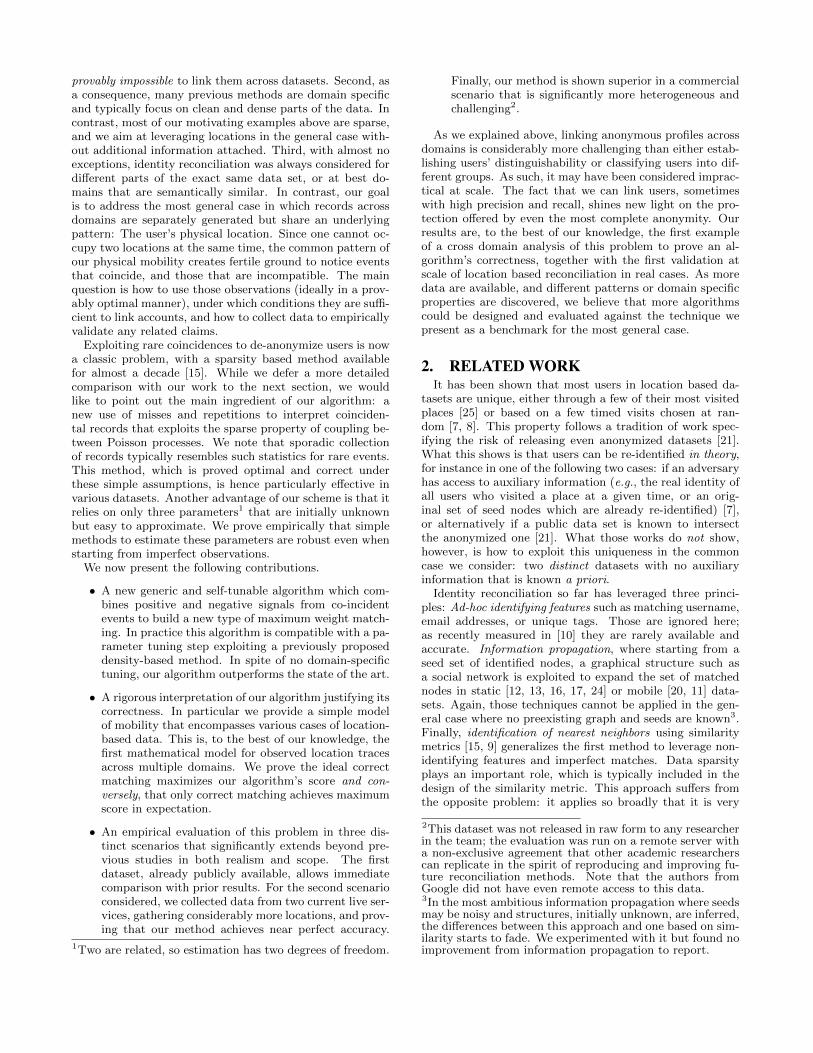
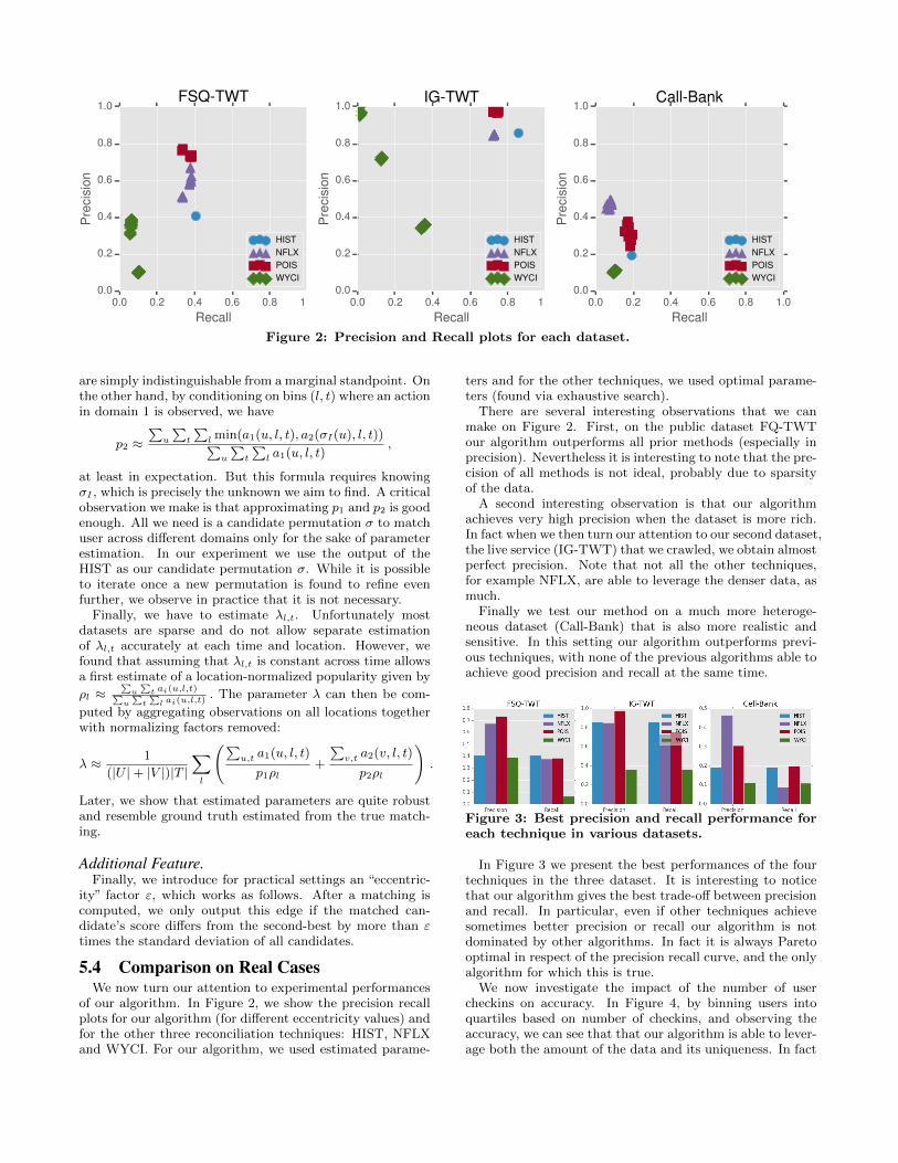
Figure 2: Precision and Recall plots for each dataset.

are simply indistinguishable from a marginal standpoint. Onthe other hand, by conditioning on bins (l, t) where an actionin domain 1 is observed, we have

p2 ≈∑u

∑t

∑l min(a1(u, l, t), a2(σI(u), l, t))∑u

∑t

∑l a1(u, l, t)

,

at least in expectation. But this formula requires knowingσI , which is precisely the unknown we aim to find. A criticalobservation we make is that approximating p1 and p2 is goodenough. All we need is a candidate permutation σ to matchuser across different domains only for the sake of parameterestimation. In our experiment we use the output of theHIST as our candidate permutation σ. While it is possibleto iterate once a new permutation is found to refine evenfurther, we observe in practice that it is not necessary.

Finally, we have to estimate λl,t. Unfortunately mostdatasets are sparse and do not allow separate estimationof λl,t accurately at each time and location. However, wefound that assuming that λl,t is constant across time allowsa first estimate of a location-normalized popularity given by

ρl ≈∑u

∑t ai(u,l,t)∑

u

∑t

∑l ai(u,l,t)

. The parameter λ can then be com-

puted by aggregating observations on all locations togetherwith normalizing factors removed:

λ ≈ 1

(|U |+ |V |)|T |∑l

(∑u,t a1(u, l, t)

p1ρl+

∑v,t a2(v, l, t)

p2ρl

).

Later, we show that estimated parameters are quite robustand resemble ground truth estimated from the true match-ing.

Additional Feature.Finally, we introduce for practical settings an “eccentric-

ity” factor ε, which works as follows. After a matching iscomputed, we only output this edge if the matched can-didate’s score differs from the second-best by more than εtimes the standard deviation of all candidates.

5.4 Comparison on Real CasesWe now turn our attention to experimental performances

of our algorithm. In Figure 2, we show the precision recallplots for our algorithm (for different eccentricity values) andfor the other three reconciliation techniques: HIST, NFLXand WYCI. For our algorithm, we used estimated parame-

ters and for the other techniques, we used optimal parame-ters (found via exhaustive search).

There are several interesting observations that we canmake on Figure 2. First, on the public dataset FQ-TWTour algorithm outperforms all prior methods (especially inprecision). Nevertheless it is interesting to note that the pre-cision of all methods is not ideal, probably due to sparsityof the data.

A second interesting observation is that our algorithmachieves very high precision when the dataset is more rich.In fact when we then turn our attention to our second dataset,the live service (IG-TWT) that we crawled, we obtain almostperfect precision. Note that not all the other techniques,for example NFLX, are able to leverage the denser data, asmuch.

Finally we test our method on a much more heteroge-neous dataset (Call-Bank) that is also more realistic andsensitive. In this setting our algorithm outperforms previ-ous techniques, with none of the previous algorithms able toachieve good precision and recall at the same time.

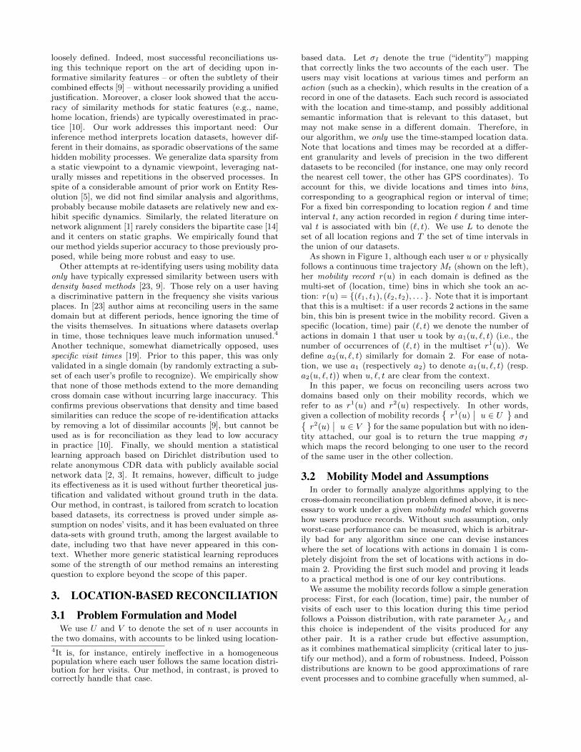
Figure 3: Best precision and recall performance foreach technique in various datasets.

In Figure 3 we present the best performances of the fourtechniques in the three dataset. It is interesting to noticethat our algorithm gives the best trade-off between precisionand recall. In particular, even if other techniques achievesometimes better precision or recall our algorithm is notdominated by other algorithms. In fact it is always Paretooptimal in respect of the precision recall curve, and the onlyalgorithm for which this is true.

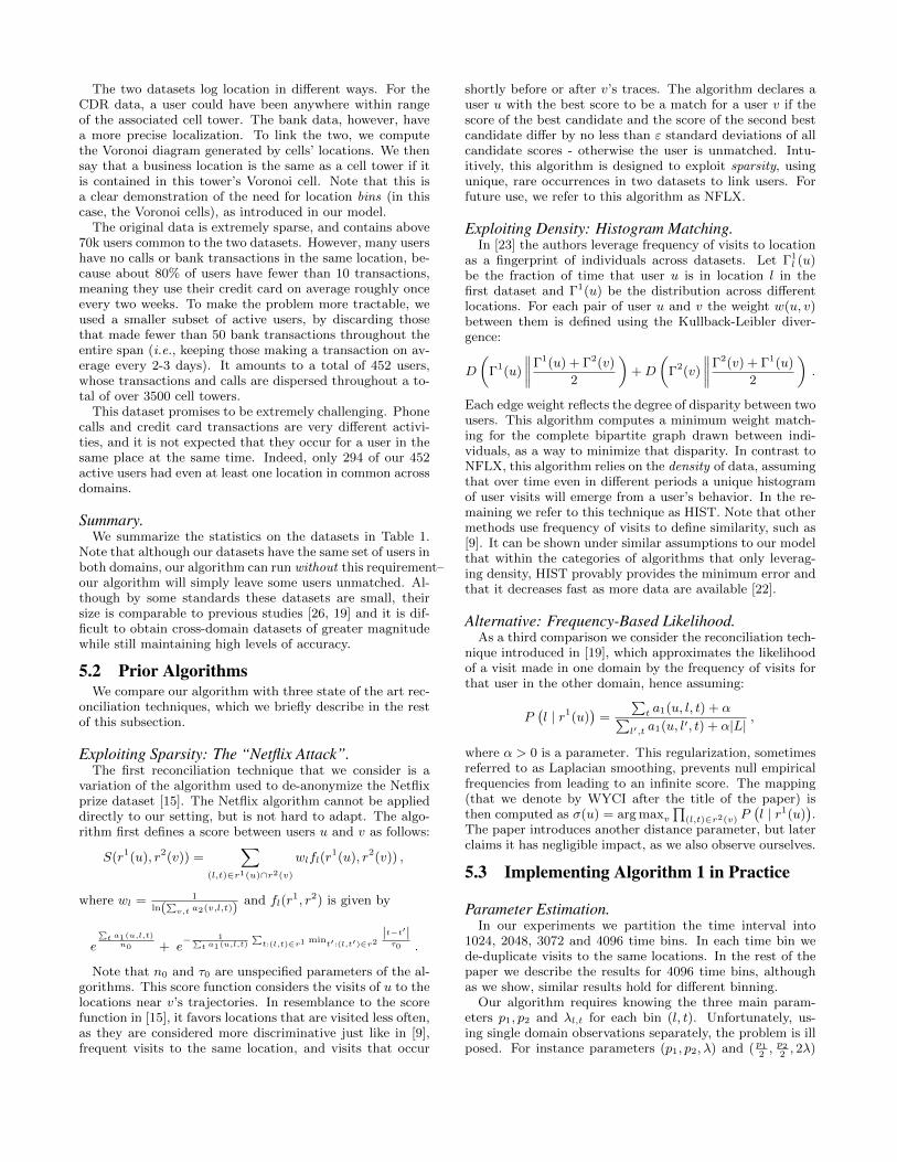
We now investigate the impact of the number of usercheckins on accuracy. In Figure 4, by binning users intoquartiles based on number of checkins, and observing theaccuracy, we can see that that our algorithm is able to lever-age both the amount of the data and its uniqueness. In fact

101

102

103

104

Checkins

0.4

0.5

0.6

0.7

0.8

Accu

racy

IG-TWT

TWT

IG

100

101

102

103

104

Checkins

0.00

0.05

0.10

0.15

0.20

0.25

0.30

0.35

0.40

0.45

Accu

racy

FSQ-TWT

TWT

FSQ

Figure 4: Number of checkins vs. our algorithm’saccuracy.

the performance of our algorithm are positively correlatedboth with the number of checkins and with the entropy ofthe visited location.

512 1024 2048 4096 8192

Timebins

0.45

0.46

0.47

0.48

0.49

0.50

0.51

0.52

F1

FSQ-TWT Time v. F1

Real params

Est. params

512 1024 2048 4096 8192

Timebins

0.76

0.78

0.80

0.82

0.84

0.86

0.88

0.90

F1

IG-TWT Time v. F1

Real params

Est. params

Figure 5: Effect of parameter estimation and timebinning on algorithm performance.

We next turn our attention to the impact of our estimatedparameters. As mentioned in Sec. 5.3, we cannot know theexact values of p1, p2, and λl,t. When running our algo-rithm, we first found a guess at a permutation, and usedthat matching to estimate the parameters. Comparing thiswith using the true permutation, we can see how far offour guess was and the impact on the algorithm. Fig. 5shows two lines, one using parameters derived from the realpermutation and one using an estimate. Clearly, using theestimate is as good as using the real permutation, and is infact better at certain time levels. Additionally, this figureshows that there is only a small boost in performance whenusing differently sized time bins. This is helpful in that itseems the algorithms performance is largely unaffected bychoice of parameters.

Figure 6: Precision and recall for the FSQ-TWTdatasets for different values of the eccentricity andvarying numbers of terms of the infinite sum.

Finally we show in Figure 6 the effect of eccentricity andnumber of terms (of the infinite sum) on performances of

our algorithm. The eccentricity is a term that rejects linksif other candidates are also very likely. A higher eccentricityshould thus correspond with greater precision at the cost oflower recall. In these figures, we can see that this relation-ship indeed holds, allowing users to potentially find only thestrongest matches, perhaps as “seed” links for other algo-rithms. The number of terms appears to have little effecton algorithm performance, empirically validating our proofthat our approximation appears to have little impact on thefinal result.

6. CONCLUSIONUser data is constantly multiplying across an increasing

array of websites, apps and services, as they are eager toshare part of their behavior with service providers to re-ceive personalized (and free) services. Users may attempt todeal with the privacy implications through partially or in-accurately filled profile information (such as entering a fakename, age, etc.), or using the privacy settings to“lock down”access. However, such methods are of limited use, becausecommonly collected fields (such as location) that are inte-gral to the service provided may in themselves be sufficientto link this account with other accounts of the same user.

In this paper, we present a new approach to character-ize when and how such linking is possible. We theoreticallyjustify our algorithm and empirically validate it on real da-tasets. The results we present, most of them shown for thefirst time in a cross-domain setting, demonstrate that sim-ple conditions may be sufficient for correct reconciliationand highlight the sensitivity of location data. Several av-enues for further research are suggested by these results:Our model assumes very simple behavior by users, model-ing them as generating location records independently, andis already quite effective. Can one further exploit patternsinherent to human mobility, such as sleep schedule, com-mute patterns, working days, and other time dependencies?Is location special, or are there other universal characteris-tics that are equally meaningful?

7. ACKNOWLEDGEMENTSThis work was supported by NSF under grant CNS-1254035.

The authors gratefully acknowledge Mat Travizano and Car-los Sarraute of Grandata for their help with this work.

8. REFERENCES

[1] M. Bayati, M. Gerritsen, D. F. Gleich, A. Saberi, andY. Wang. Algorithms for Large, Sparse NetworkAlignment Problems. Data Mining, 2009. ICDM ’09.Ninth IEEE International Conference on, pages705–710, 2009.

[2] A. Cecaj, M. Mamei, and N. Bicocchi.Re-identification of anonymized CDR datasets usingsocial network data. In Pervasive Computing andCommunications Workshops (PERCOM Workshops),2014 IEEE International Conference on, pages237–242. IEEE, 2014.

[3] A. Cecaj, M. Mamei, and F. Zambonelli.Re-identification and information fusion betweenanonymized CDR and social network data. Journal ofAmbient Intelligence and Humanized Computing,7(1):1–14, 2015.

[4] E. Cho, S. A. Myers, and J. Leskovec. Friendship andmobility: user movement in location-based socialnetworks. In KDD ’11: Proceedings of the 17th ACMSIGKDD international conference on Knowledgediscovery and data mining, pages 1082–1090. ACMRequest Permissions, 2011.

[5] P. Christen. Data Matching, Concepts and Techniquesfor Record Linkage, Entity Resolution, and DuplicateDetection . Springer Berlin Heidelberg, Berlin,Heidelberg, 2012.

[6] D. J. Crandall, L. Backstrom, D. Cosley, S. Suri,D. Huttenlocher, and J. M. Kleinberg. Inferring socialties from geographic coincidences. Proceedings of theNational Academy of Sciences, 107(52):22436–22441,2010.

[7] Y.-A. de Montjoye, C. A. Hidalgo, M. Verleysen, andV. D. Blondel. Unique in the Crowd: The privacybounds of human mobility. Scientific Reports, 3, 2013.

[8] Y.-A. de Montjoye, L. Radaelli, V. K. Singh, and A. S.Pentland. Unique in the shopping mall: on thereidentifiability of credit card metadata. Science,347(6221):536–539, 2015.

[9] O. Goga, H. Lei, S. Parthasarathi, and G. Friedland.Exploiting innocuous activity for correlating usersacross sites. In WWW ’13: Proceedings of the 22ndinternational conference on World Wide Web, pages447–458, 2013.

[10] O. Goga, P. Loiseau, R. Sommer, R. Teixeira, andK. Gummadi. On the Reliability of Profile MatchingAcross Large Online Social Networks. In KDD ’15:Proceedings of the 21th ACM SIGKDD InternationalConference on Knowledge Discovery and Data Mining,pages 1799–1808. ACM Request Permissions, 2015.

[11] S. Ji, W. Li, M. Srivatsa, J. S. He, and R. Beyah.Structure Based Data De-Anonymization of SocialNetworks and Mobility Traces. In ISC Proceedings ofthe 17th International Information SecurityConference, pages 237–254. Springer InternationalPublishing, 2014.

[12] E. Kazemi, S. H. Hassani, and M. Grossglauser.Growing a graph matching from a handful of seeds.Proceedings of the VLDB Endowment,8(10):1010–1021, 2015.

[13] N. Korula and S. Lattanzi. An efficient reconciliationalgorithm for social networks. Proceedings of VLDB,7(5):377–388, 2014.

[14] D. Koutra, H. Tong, and D. Lubensky. BIG-ALIGN:Fast Bipartite Graph Alignment. In Data Mining(ICDM), 2013 IEEE 13th International Conferenceon, pages 389–398, 2013.

[15] A. Narayanan and V. Shmatikov. RobustDe-anonymization of Large Sparse Datasets. Securityand Privacy, 2008. SP 2008. IEEE Symposium on,pages 111–125, 2008.

[16] A. Narayanan and V. Shmatikov. De-anonymizingSocial Networks. Security and Privacy, 2009 30thIEEE Symposium on, pages 173–187, 2009.

[17] P. Pedarsani and M. Grossglauser. On the privacy ofanonymized networks. In KDD ’11: Proceedings of the17th ACM SIGKDD international conference onKnowledge discovery and data mining, pages1235–1243. ACM Request Permissions, 2011.

[18] C. J. Riederer, S. Zimmeck, C. Phanord,A. Chaintreau, and S. M. Bellovin. I don’t have aphotograph, but you can have my footprints.:Revealing the Demographics of Location Data. InCOSN ’15: Proceedings of the third ACM conferenceon Online social networks, pages 185–195. ACM, 2015.

[19] L. Rossi and M. Musolesi. It’s the Way you Check-in:Identifying Users in Location-Based Social Networks.COSN ’14: Proceedings of the 2nd ACM conference onOnline social networks, pages 215–226, 2014.

[20] M. Srivatsa and M. Hicks. Deanonymizing MobilityTraces: Using Social Networks as a Side-Channel.CCS ’12: Proceedings of the 2012 ACM conference onComputer and communications security, pages628–637, 2012.

[21] L. Sweeney. k-anonymity: a model for protectingprivacy. International Journal of Uncertainty,Fuzziness and Knowledge-Based Systems,10(5):557–570, 2002.

[22] J. Unnikrishnan. Asymptotically Optimal Matching ofMultiple Sequences to Source Distributions andTraining Sequences. Information Theory,61(1):452–468, 2015.

[23] J. Unnikrishnan and F. M. Naini. De-anonymizingprivate data by matching statistics. InCommunication, Control, and Computing (Allerton),2013 51st Annual Allerton Conference on, pages1616–1623. IEEE, 2013.

[24] L. Yartseva and M. Grossglauser. On the performanceof percolation graph matching. In COSN ’15:Proceedings of the third ACM conference on Onlinesocial networks, pages 119–130. ACM RequestPermissions, 2013.

[25] H. Zang and J. Bolot. Anonymization of location datadoes not work: a large-scale measurement study. InMobiCom ’11: Proceedings of the 17th annualinternational conference on Mobile computing andnetworking, pages 145–156. ACM RequestPermissions, 2011.

[26] J. Zhang, X. Kong, and P. S. Yu. Transferringheterogeneous links across location-based socialnetworks. In WSDM ’14: Proceedings of the 7th ACMinternational conference on Web search and data

mining, pages 303–312. ACM Request Permissions,2014.

[27] Y. Zhong, N. J. Yuan, W. Zhong, F. Zhang, andX. Xie. You Are Where You Go. In WSDM ’15:Proceedings of the 8th ACM international conferenceon Web search and data mining, pages 295–304. ACMPress, 2015.

9. APPENDIX

9.1 Proof of Theorem 1We first show that each of the 2 factors in the denominator

of φ(a1, a2) can be replaced by the corresponding truncatedsum while affecting its value by at most 1 + 1/C2. Sincethe numerator is decreased by truncation, this establishesthe upper bound on φ′(a1, a2). We then show that for thenumerator of φ(a1, a2), the difference between the infinitesum and its truncated version is at most 1/C times the firstterm in this sum. Since the denominator is decreased bytruncation, this establishes the lower bound on φ′.

To obtain the upper bound, we first consider the factor∑∞k=a1

λk

k!

(ka1

)(1 − p1)k−a1 in the denominator. Expanding

the binomial coefficient and pulling common terms outsidethe summation, this factor can be written as:

λa1

a1!

∑k≥a1

λk−a1(1− p1)k−a1

(k − a1)!=λa1

a1!

∑k≥0

λk(1− p1)k

k!

Note that first term in this revised sum evaluates to 1, theterm of index lnC evaluates to λlnC(1 − p1)lnC/(lnC)! �1C2 , and the sum of all terms from lnC onward are at mostλlnC(1−p1)lnC/(lnC)!

(1−λ) (upper bounding the infinite sum with

a geometric series). Since λ < 1/2, we conclude that thesum of all terms from index lnC onward are less than 1/C2

times the first term.The truncated sum for the second factor in the denomina-

tor can be bounded identically, giving us the desired upperbound on φ′(a1, a2).

It remains only to establish the lower bound by boundingthe truncated numerator. We assume without loss of gen-erality that a1 ≥ a2. Expanding the binomial coefficientsin the definition of the numerator of φ(a1, a2) and pullingcommon terms outside the summation, we can rewrite thenumerator as:

λa1(1− p2)(a1−a2)

a1! a2!

∑k≥a1

λk−a1 ((1− p1)(1− p2))k−a1 · k!

(k − a1)!(k − a2)!

The first term inside the revised sum is simply a1!/(a1 −a2)! > 1. Let i denote the final index in the truncatedsum, a1 + max{lnC, 2a1}. The ith term is upper boundedby λi−a1 · i!

(i−a1)!(i−a2)!. If a1 ≥ 4, then since i ≥ 3a1, it

is easy to see that i!(i−a1)!2

< 1/2. If a1 ≤ 4, then since

i − a1 ≥ lnC ≥ 7 , we can note that i!(i−a1)!2

< 1/2. As

λ < 1/2 and i > a1+lnC, the ith term is less than 1/C ·1/2.Again upper bounding the infinite sum with a geometricseries, the sum of all terms from index i onward is less thanthe ith term divided by (1−λ), and hence < 1/C. Therefore,the sum of all terms from the ith term onward is less than1/C times the first term, completing the proof.

9.2 Proof of Lemma 2Recall that in Lemma 2, we proved that E[Score(u, v, `, t] ≤

0 for any pair of users u, v such that v 6= σI(u). For v =σI(u), we showed that the expected score is lower boundedby:

X(0, 0) lnX(0, 0)

Y (0, 0)+ (1−X(0, 0)) ln

(1−X(0, 0))

(1− Y (0, 0))

= X(0, 0) lnX(0, 0)

Y (0, 0)− (1−X(0, 0)) ln

(1− Y (0, 0))

(1−X(0, 0))

≥ (1− λ(p1 + p2 − p1p2))λp1p2 −

λ(p1 + p2 − p1p2) ln(1− e−λ(p1+p2))

(1− e−λ(p1+p2−p1p2))

To prove that this expression is lower bounded by (λp1p2)2K,it suffices to prove that:

(1− λ(p1 + p2 − p1p2))λp1p2 −

λ(p1 + p2 − p1p2) ln(1− e−λ(p1+p2))

1− e−λ(p1+p2−p1p2))≥ (λp1p2)2K

or equivalently:

(1− λ(p1 + p2 − p1p2))p1p2 − λ(p1p2)2K

− (p1 + p2 − p1p2) ln(1− e−λ(p1+p2))

(1− e−λ(p1+p2−p1p2))≥ 0 (2)

We can simplify the final factor in this inequality as follows:

ln(1− e−λ(p1+p2))

(1− e−λ(p1+p2−p1p2))= ln e−λ(p1p2)

(eλ(p1+p2) − 1)

(eλ(p1+p2−p1p2) − 1)

=

(ln

(eλ(p1+p2) − 1)

(eλ(p1+p2−p1p2) − 1)

)− λp1p2

where the first equality came from multiplying the numera-tor and denominator by eλ(p1+p2−p1p2).Substituting into Inequality (2), our lemma reduces to:

(1− λ(p1 + p2 − p1p2))p1p2 − λ(p1p2)2K

(p1 + p2 − p1p2)

(ln

(eλ(p1+p2) − 1)

(eλ(p1+p2−p1p2) − 1)− λp1p2

)≥ 0

or, equivalently:

p1p2(1− λ(p1p2)K)−

(p1 + p2 − p1p2) ln(eλ(p1+p2) − 1)

(eλ(p1+p2−p1p2) − 1)≥ 0 (3)

This is hard to simplify directly, so we introduce the fol-lowing upper bound:

λp1p2 = ln1

e−λp1p2= ln

eλ(p1+p2)

eλ(p1+p2−p1p2)≤ ln

eλ(p1+p2) − 1

eλ(p1+p2−p1p2) − 1

Using Z to represent the quantity ln eλ(p1+p2)−1

eλ(p1+p2−p1p2)−1and

substituting the new inequality in Inequality (3), we are try-

ing to prove:

p1p2(1− ZK)− (p1 + p2 − p1p2)Z ≥ 0

⇔ p1p2 ≥ (p1 + p2 − p1p2(1−K))Z

⇔ p1p2p1 + p2 − p1p2(1−K)

≥ Z

⇔ ep1p2

p1+p2−p1p2(1−K) ≥ eλ(p1+p2) − 1

eλ(p1+p2−p1p2) − 1

Now to conclude the proof we use two inequalities thatfollows from the Taylor expansions. In particular we have:

ex ≥ 1 + x+1

2x2

and for x ∈ o(1):

ex ≤ 1 + x+ x2

Now by assuming that λ ∈ o(1) and by fixingK = 12λ(p1+

p2 − p1p2)2 we get:

ep1p2

p1+p2−p1p2(1−K) ≥ eλ(p1+p2) − 1

eλ(p1+p2−p1p2) − 1

⇔ 1 +p1p2

p1 + p2 − p1p2 + 12λ(p1 + p2 − p1p2)2

+

p21p22

2(p1 + p2 − p1p2 + 12λ(p1 + p2 − p1p2)2)2

≥

λ(p1 + p2) + λ2(p1 + p2)2

λ(p1 + p2 − p1p2 + 12λ(p1 + p2 − p1p2)2)

⇔ 1 +p1p2

p1 + p2 − p1p2 + 12λ(p1 + p2 − p1p2)2

+

p21p22

2(p1 + p2 − p1p2 + 12λ(p1 + p2 − p1p2)2)2

≥

1 +p1p2 + λ(p1 + p2)2

p1 + p2 − p1p2 + 12λ(p1 + p2 − p1p2)2

⇔12p21p

22

p1 + p2 − p1p2 + 12λ(p1 + p2 − p1p2)2

≥ λ(p1 + p2)2

Now by fixing λ < 18

p21p22

(p1+p2)2we get:

12p21p

22

p1 + p2 − p1p2 + 12λ(p1 + p2 − p1p2)2

≥ λ(p1 + p2)2

⇔12p21p

22

p1 + p2 − p1p2 + 116p21p

22

≥ 1

8p21p

22

⇔ 1

4p21p

22 ≥

1

8p21p

22

So the claim follows.