link.springer.com · Eur. Phys. J. C (2013) 73:2453 DOI 10.1140/epjc/s10052-013-2453-3 Regular...

Eur. Phys. J. C (2013) 73:2453DOI 10.1140/epjc/s10052-013-2453-3

Regular Article - Experimental Physics

An update of the HLS estimate of the muon g − 2

M. Benayoun1,a, P. David1, L. DelBuono1, F. Jegerlehner2,3

1LPNHE des Universités Paris VI et Paris VII, IN2P3/CNRS, 75252 Paris, France2Institut für Physik, Humboldt–Universität zu Berlin, Newtonstrasse 15, 12489 Berlin, Germany3Deutsches Elektronen–Synchrotron (DESY), Platanenallee 6, 15738 Zeuthen, Germany

Received: 26 October 2012 / Revised: 29 April 2013 / Published online: 5 June 2013© The Author(s) 2013. This article is published with open access at Springerlink.com

Abstract A global fit of parameters allows us to pin downthe Hidden Local Symmetry (HLS) effective Lagrangian,which we apply for the prediction of the leading hadronicvacuum polarization contribution to the muon g − 2. Thelatter is dominated by the annihilation channel e+e− →π+π−, for which data are available by scan (CMD-2 &SND) and ISR (KLOE-2008, KLOE-2010 & BaBar) ex-periments. It is well known that the different data sets arenot in satisfactory agreement. In fact it is possible to fixthe model parameters without using the π+π− data, by us-ing instead the dipion spectra measured in the τ -decays to-gether with experimental spectra for the π0γ , ηγ , π+π−π0,K+K−, K0K0 final states, supplemented by specific mesondecay properties. Among these, the accepted decay widthfor ρ0 → e+e− and the partial widths and phase informationfor the ω/φ → π+π− transitions, are considered. It is thenshown that, relying on this global data set, the HLS model,appropriately broken, allows to predict accurately the pionform factor below 1.05 GeV. It is shown that the data sam-ples provided by CMD-2, SND and KLOE-2010 behaveconsistently with each other and with the other considereddata. Consistency problems with the KLOE-2008 and BaBardata samples are substantiated. “All data” global fits are in-vestigated by applying reweighting the conflicting data sets.Constraining to our best fit, the broken HLS model yieldsathμ = (11 659 169.55+ [+1.26

−0.59

]φ+ [+0.00

−2.00

]τ±5.21th) 10−10

associated with a very good global fit probability. Corre-spondingly, we find that aμ = a

expμ − ath

μ exhibits a sig-nificance ranging between 4.7 and 4.9σ .

1 Introduction

The theoretical value for the muon anomalous magnetic mo-ment aμ is an important window in the quest for new phe-nomena in particle physics. The predicted value is the sum

a e-mail: [email protected]

of several contributions and the most prominent ones are al-ready derived from the Standard Model with very high ac-curacies. The QED contribution is thus estimated with anaccuracy of a few 10−12 [1–3] and the precision of the elec-troweak contribution is now of order 10−11 [4]. The light-by-light contribution to aμ is currently known with an ac-cepted accuracy of 2.6 × 10−10 [5].

Presently, the uncertainty of the Standard Model predic-tion for aμ is driven by the uncertainty on the leading order(LO) hadronic vacuum polarization (HVP) up to �2 GeV[6, 7]. This region is covered by the non-perturbative regimeof QCD and the leading order HVP (LO-HVP) is evaluatedby means of:

⎧⎪⎪⎪⎨

⎪⎪⎪⎩

aLO-HVPμ =

∑

i

aμ(Hi),

aμ(Hi) = 1

4π3

∫ scut

sHi

ds K(s)σHi(s),

(1)

which relates the hadronic intermediate state contribu-tions {Hi, i = 1, . . . , n} to the annihilation cross sectionsσ(e+e− → Hi) ≡ σHi

(s). K(s) is a known kernel [4] en-hancing the weight of the threshold region sHi

and scut issome energy squared where perturbative QCD starts to beapplicable. In the region where perturbative QCD holds,1 itscontribution to aμ carries an uncertainty of the order of afew 10−11.

Up to very recently, the single method used to get theaμ(Hi)’s was to plug the experimental cross sections intoEq. (1). Among the most recent studies based on thismethod, let us quote [6–9]. When several data sets cover thesame cross section σHi

(s), Eq. (1) is used with some appro-priate weighting of the various spectra, allowing to improvethe corresponding aμ(Hi).

1The charmonium and bottomium regions carry uncertainties also inthe range of a few 10−11.

mailto:[email protected]

of 41 Eur. Phys. J. C (2013) 73:2453

On the other hand, it is now widely accepted that theVector Meson Dominance (VMD) concept applies to lowenergy physics [10, 11]. VMD based Effective Lagrangianshave been proposed like the Resonance Chiral PerturbationTheory or the Hidden Local Symmetry (HLS) Model; it hasbeen proven [12] that these are essentially equivalent. Intrin-sically, this means that there exist physics correlations be-tween the various e+e− → Hj annihilation channels. There-fore, it becomes conceptually founded to expect improvingeach aμ(Hi) by means of the data covering the other chan-nels e+e− → Hj (j �= i).

This is basically the idea proposed in [13] relying on theHLS model [14, 15]. Using a symmetry breaking mecha-nism based on the simple BKY idea [16] and a vector me-son mixing scheme, the model has been developed stepwise[17–20] and its most recent form [13] has been shown toprovide a successful simultaneous description of the e+e−annihilation into the π+π−, π0γ , ηγ , π+π−π0, K+K−,

K0K0

final states as well as the τ± → ντπ±π0 decay spec-

trum. Some more decays of the form2 V → Pγ or P → γ γ

are considered.As higher mass meson nonets are absent from the stan-

dard HLS model, its energy scope is a priori limited upwardsby the φ meson mass region (�1.05 GeV). However, as thisregion contributes more than 80 % to the total HVP, im-provements which can follow from the broken HLS modelare certainly valuable.3

The global simultaneous fit of the data corresponding tothe channels quoted above allows to reconstruct the variouscross sections σHi

(s) taking automatically into account thephysics correlations inside the set H ≡ {Hi} of possible finalstates and decay processes. The fit parameter values and theparameter error covariance matrix summarize optimally thefull knowledge of H. This has two important consequences:

• One should get the {aμ(Hi), i = 1, . . . , n} with improveduncertainties by integrating the model cross sections in-stead of the measured ones. Indeed, the functional cor-relations among the various cross sections turn out toprovide (much) larger statistics in each channel and thusyield improved uncertainties for each aμ(Hi).

• When several data samples cover the same process Hi ,one has a handle to motivatedly examine the behavior ofeach within the global fit context. Stated otherwise, theissue of the consistency of each data set with all the otherscan be addressed with the (global) fit probability as a toolto detect data samples carrying problematic properties.

2We denote by V or P resp. any meson belonging to the (basic) vectoror pseudoscalar lowest mass nonets.3The broken HLS model does not include the 4π , 5π , 6π , ηππ andωπ annihilation channels. Therefore, the (small) contribution of thesemissing channels [13] to aμ should be still evaluated by direct integra-tion of the experimental cross sections; up to the φ mass, this amountsto [13] (1.55 ± 0.57tot) × 10−10.

Up to now, the broken HLS model (BHLS) [13]—basically an empty shell—has been fed with all existing datasets4 for what concerns the annihilation channels π0γ , ηγ ,

π+π−π0, K+K−, K0K0, with the spectra from ALEPH

[21], CLEO [22] and BELLE [23] for the τ dipion decay5

and with the V Pγ/Pγ γ partial width information extractedfrom the Review of Particle Properties (RPP) [24]. This al-ready represents more than 40 data sets collected by differ-ent groups with different detectors; one may thus considerthat the systematics affecting these data sets wash out to alarge extent within a global fit framework.

For what concerns the crucial process e+e− → π+π−,the analysis in [13] only deals with the data sets collected inthe scan experiments performed at Novosibirsk and referredto globally hereafter as NSK [25–29]. The main reason was,at this step, to avoid discussing the reported tension [8, 30]between the various existing π+π− data sets: the scan datasets just quoted, and the data sets collected using the InitialState Radiation (ISR) method by KLOE [31, 32] and BaBar[33, 34], not to mention the pion form factor data collectedin the spacelike region [35, 36].

It has thus been shown that the global fit excluding theISR data sets, allows to yield a splendid fit quality; thisproves that the whole collection of data sets considered in[13] is self-consistent and may provide a safe reference, i.e.a benchmark, to examine the behavior of other data samples.

Using the fit results, the uncertainty on the contributionto aμ of each of the annihilation channels considered wasimproved by—at least—a factor of 2, compared to the stan-dard estimation method based on the numerical integrationof the measured cross sections. For the case of the π+π−channel, the final uncertainty was even found slightly betterthan those obtained with the standard method by mergingscan and ISR data, i.e. a statistics about 4 times larger in theπ+π− annihilation channel.

The main purpose of the present study is an update of thework in [13] aiming at confronting all scan (NSK) and ISR(from BaBar and KLOE)—and even spacelike [35, 36]—π+π− data and reexamine the reported issues [8, 30]. Theframework in which our analysis is performed is the sameas the one motivated and developed in [13].

The broken HLS model described in [13] happens toprovide a tool allowing to compare the behavior of anyof these π+π− data sets when confronted with the π0γ ,

ηγ , π+π−π0, K+K−, K0K0

annihilation data and withthe τ dipion spectra. Indeed, the latter data alone, supple-mented with some limited information extracted from the

4The full list of data sets can be found in [19] or [13] together with acritical analysis of their individual behavior.5The energy region used in the fits has been limited to the[2mπ,1 GeV] interval where the three data sets are in accord with eachother. This should lessen the effect of some systematic effects.

Eur. Phys. J. C (2013) 73:2453 of 41

Review of Particle Properties6 (RPP) [24], allow to predictthe pion form factor with a surprisingly good precision. Theadditional RPP information is supposed to carry the IsospinBreaking (IB) information requested in order to derive re-liably the π+π− information from the knowledge of theπ±π0 spectrum.

We also take profit of the present work to update the nu-merical values for some contributions to the muon anoma-lous moment aμ, all gathered in Table 10 of [13]. Thus,we update the QED entry by using the recent spectacularprogress by Aoyama, Hayakawa, Kinoshita and Nio [1, 2].They have been able to perform a complete numerical cal-culation of the 5-loop QED corrections to ae and aμ. On theother hand, the electroweak contribution, which depends onthe Higgs mass at 2-loops is now better known if we acceptthat ATLAS [37] and CMS [38] have observed at the LHCthe Higgs boson at a mass of about 125 GeV in a narrowwindow. Using this information slightly changes the centralvalue as well as the uncertainty of the EW entry. We alsohave reevaluated the higher order HVP contribution (HO)within the standard approach based on all π+π− channels(i.e. all scan and ISR data).

The paper is organized as follows. Section 2 reminds themotivations of the BHLS model and a few basic topics con-cerning the ππ channel description (from [13]); we alsoreexamines how the isospin breaking corrections apply. InSect. 3, the detailed framework—named “τ + PDG”—usedto study the differential behavior of the scan and ISR datais presented. Thanks to the (wider than usual) energy rangecovered by the BaBar spectrum [33, 34], a detailed studyof the π+π− spectrum in the φ region can be performed forthe first time. This leads to update the φ → π+π− treatmentwithin our computer code; this is emphasized in Sect. 3.3.In Sect. 4, one confronts the “τ + PDG” predictions withthe available scan (NSK) and ISR data samples; it is shownthat the NSK data and both KLOE data samples (referred tohereafter as KLOE08 [31] and KLOE10 [32]) have similarproperties while BaBar behaves differently, especially in theρ − ω interference region. Section 5, especially Sect. 5.1,reports on the global fits performed using the various π+π−data samples each in isolation or combined. Section 5.2 col-lects some topics on various aspects of the physics coveredby the HLS model. More precisely, Sect. 5.2.1 is devoted tostudying the φ region of the pion form factor and Sect. 5.2.2gives numerical fit information which may allow to comparewith corresponding results available from other studies per-formed using different methods. In Sect. 6, we focus on theconsequences for the muon anomalous moment aμ of thevarious scan and ISR π+π− spectra and compare resultswith the BNL [39, 40] measurement. The π+π− intermedi-ate state contribution to aμ from the invariant mass region

6We occasionally refer to the RPP as Particle Data Group (PDG).

[0.630,0.958] GeV is especially considered as it serves toexamine the outcome of various fits with respect to the ex-perimental expectations. Finally, Sect. 7 is devoted to con-clusions.

2 A brief reminder of concern for the ππ channel

2.1 The general context of the HLS model

At very low energies chiral perturbation theory (ChPT)[41, 42] is the “from first principles” approach to low-energyhadron physics. Unfortunately, ChPT ceases to converge atenergies as low as about 400 MeV, and thus the most impor-tant region of the spin 1 resonances fails to be in the scopeof ChPT.

A phenomenologically well established description of thevector mesons is the VMD model, which may be neatlyput into a quantum field theory (QFT) framework. This,however, has to be implemented in accord with the chi-ral structure of the low energy spectrum. It is now widelyaccepted that a low energy effective QFT of massive spin1 bosons must be a Yang–Mills theory supplemented witha Higgs–Kibble mechanism. The general framework is theResonance Chiral Perturbation Theory (RChPT) [10], anextension of ChPT to vector mesons usually expressed inthe (not very familiar) antisymmetric tensor field formalism.Like in ChPT, the basic fields are the unitary matrix fieldsξL,R = exp[±i P/fπ ], where P = P8 +P0 is the SU(3) ma-trix of pseudoscalar fields, with P0 and P8 being respec-tively the basic singlet and octet pseudoscalar field matrices.

The Hidden Local Symmetry (HLS) ansatz [14, 15] isan extension of the ChPT non-linear sigma model to a non-linear chiral Lagrangian based on the symmetry patternGglobal/Hlocal, where G = SU(3)L ⊗ SU(3)R is the chiralgroup of QCD and H = SU(3)V is the vector subgroup. Thehidden local SU(3)V requires the vector meson fields, repre-sented by the SU(3) matrix field Vμ, to be gauge fields. Thecorresponding covariant derivative reads Dμ = ∂μ − i g Vμ

and can be naturally extended [15] in order to include thecouplings to the electroweak gauge fields Aμ, Zμ and W±

μ .It has been proven in [12] that RChPT and HLS are equiv-

alent provided consistency with the QCD asymptotic behav-ior is incorporated. Such an extension of ChPT to includeVMD structures is fundamental. Although it is not yet estab-lished which version is the true low-energy effective QCD,it is the widely accepted framework which includes all par-ticles as effective fields up to the φ and only confrontationwith data can tell to which extent such an effective theoryworks. This has been the subject of the study [13] whichwe update by extending it. Obviously, this approach is morecomplicated than a Gounaris–Sakurai ansatz and requireselaborate calculations because the basic symmetry group is

of 41 Eur. Phys. J. C (2013) 73:2453

not SU(2) but SU(3) × SU(3) where the SU(3) vector sub-group must be gauged in order to obtain the Yang–Millsstructure for the spin 1 bosons.

All relevant states have to be incorporated in accord withthe chiral structure of the low-energy hadron spectrum. Ina low-energy expansion, one naturally expects the leadinglow-energy tail to be close to a renormalizable effectivetheory; however, this is not true for the pseudo Nambu–Goldstone boson sector, which is governed by a non-linearσ model, rather than by a renormalizable linear σ model.The reason is that the latter requires a scalar (σ ) meson asa main ingredient. Phenomenologically, scalars only play akind of “next-to-leading” role.

The situation is quite different for the spin 1 bosons,which naturally acquire a Yang–Mills effective structure ina low-energy expansion i.e., they naturally exhibit a lead-ing local gauge symmetry structure with masses as gener-ated by a Higgs–Kibble mechanism. There is one importantproviso, however: such a low-energy effective structure ispronounced only to the extent that the effective expansionscale Λeff is high enough, which is not clear at all for QCDunless we understand why Λeff � ΛOCD ∼ 400 MeV. How-ever, there is a different approach, namely, a “derivation” ofthe Extended Nambu–Jona–Lasinio (ENJL) model [43, 44],which has also been proved to be largely equivalent to theResonance Lagrangian Approach (RLA) [45, 46]. Last butnot least, large-Nc QCD [47–50] in fact predicts the low en-ergy hadron spectrum to be dominated by spin 1 resonances.These arguments are also the guidelines for the construc-tion of the HLS model [14, 15]. It provides a specific wayto incorporate the phenomenologically known low energyhadron spectrum into an effective field theory.

Most frequently the RLA is applied to study individualprocesses. In this paper as in a few previous ones, we at-tempt to fit the whole HLS Lagrangian by a global fit strat-egy. This is, in our opinion, the only way to single out aphenomenologically acceptable low-energy effective theory,which allows to make predictions which can be confrontedwith experiments.

2.2 The broken HLS Lagrangian

The (unbroken) HLS Lagrangian is then given by LHLS =LA + aLV , where

LA/V = −f 2π

4Tr[L ± R]2,

(ξL,R = exp[±i P/fπ ]) (2)

with L = [DμξL]ξ†L and R = [DμξR]ξ†

R ; a is a basic HLSparameter not fixed by the theory, which should be con-strained by confrontation with the data. From standard VMDmodels, one expects a � 2.

It is well known that the global chiral symmetry Gglobal isnot realized as an exact symmetry in nature, which implies

that the ideal HLS symmetry is evidently not a symmetry ofnature either. Therefore, it has obviously to be broken appro-priately in order to provide a realistic low energy effectivetheory mimicking low energy effective QCD.

Unlike in ChPT where one is performing a system-atic low energy expansion in low momenta and the quarkmasses, here one introduces symmetry breaking as phe-nomenological parameters to be fixed from appropriate data.Since a systematic low energy expansions à la ChPT doesnot converge above about �400 MeV, this is the only wayto model phenomenology up to, and including, the φ reso-nance region.

In our approach, the Lagrangian pieces in Eqs. (2) arebroken in a two step procedure. A first breaking mechanismnamed BKY is used, originating from [15, 16]. In orderto avoid some undesirable properties [51, 52] of the origi-nal BKY mechanism, we have adopted the modified BKYscheme proposed in [17]. In its original form, this modi-fied BKY breaking scheme only covers the breaking of theSU(3) symmetry; following [53], it has been extended in or-der to include isospin symmetry breaking effects. This turnsout to modify Eqs. (2) by introducing two constant diagonalmatrices XA/V :

LA/V =⇒ L′A/V = −f 2

π

4Tr

{[L ± R] XA/V

}2 (3)

and the (non-zero) entries in XA/V are fixed from fit to thedata. The final broken HLS Lagrangian can be written:

L′HLS = L′

A + aL′V + L’t Hooft. (4)

One has, here, included L’t Hooft which provides determi-nant terms [54] breaking the nonet symmetry in the pseu-doscalar sector and thus allowing an improved account ofthe π0, η, η′ sector. L′

HLS can be found expanded in the var-ious Appendices of [13].

However, in order to account successfully for the largestpossible set of data, isospin symmetry breaking à la BKYshould be completed by a second step involving the kaonloop mixing of the neutral vector mesons (ρ0

I , ωI and φI )outlined just below. This implies a change of fields to beperformed in the L′

HLS Lagrangian.

2.3 Mixing of neutral vector mesons through kaon loops

It has been shown [13, 19, 20] that L′HLS is insufficient in

order to get a good simultaneous account of the e+e− →π+π− annihilation data and of the dipion spectrum mea-sured in the τ± → ντπ

±π0 decay. A consistent solution tothis problem is provided by the vector field mixing mecha-nism first introduced in [18].

Basically, the vector field mixing is motivated by the one-loop corrections to the vector field squared mass matrix.

Eur. Phys. J. C (2013) 73:2453 of 41

These are generated by the following term of the brokenHLS Lagrangian7 L′

HLS:

iag

4zA

{[ρ0

I + ωI − √2zV φI

]K− ↔

∂ K+

+ [ρ0

I − ωI + √2zV φI

]K0 ↔

∂ K0}

, (5)

where g is the universal vector coupling and the subscriptI indicates the ideal vector fields originally occurring in theLagrangian.

Therefore, the vector meson squared mass matrix M20 ,

which is diagonal at tree level, undergoes corrections atone-loop. The perturbation matrix δM2(s) [18–20] de-pends on the square of the momentum flowing throughthe vector meson lines. The diagonal entries acquire self-mass corrections—noticeably the ρ0 entry absorbs the pionloop—but non-diagonal entries are also generated whichcorrespond to transitions among the ideal ρ0, ω and φ mesonfields which originally enter the HLS Lagrangian:8 Πωφ(s),Πρω(s) and Πρφ(s). These are linear combinations of thekaon loops.9 Denoting by resp. Πc(s) and Πn(s) the chargedand the neutral kaon loops (including resp. the ρ0K+K−and ρ0K0K0 coupling constants squared), one defines twocombinations of these:

ε1(s) = Πc(s) − Πn(s), ε2(s) = Πc(s) + Πn(s). (6)

In term of ε1(s) and ε2(s), the transition amplitudeswrite:

Πωφ(s) = −√2zV ε2(s), Πρω(s) = ε1(s),

Πρφ(s) = −√2zV ε1(s).

(7)

Therefore, at one-loop order, the ideal vector field VI =[ρ0

I , ωI , φI ] originally occurring in L′HLS are no longer

mass eigenstates; the physical vector fields are then (re)de-fined as the eigenvectors of M2 = M2

0 + δM2(s). Thischange of fields should be propagated into the whole bro-ken HLS Lagrangian L′

HLS, extended in order to include theanomalous couplings [55] as done in [13]. In terms of thecombinations (VR1) of the original vector fields VI which

7For clarity, we have dropped out the isospin breaking corrections gen-erated by the BKY mechanism; the exact formula can be found in theAppendix A of [13]. The parameter zV corresponds to the breaking ofthe SU(3) symmetry in the Lagrangian piece LV , while zA is associ-ated with the SU(3) breaking of LA. zV has no really intuitive value,while zA can be expressed in terms of the kaon and pion decay con-stants as zA = [fK/fπ ]2.8These mixing functions were denoted resp. εωφ(s), ερω(s) and ερφ(s)

in Sect. 6 of [13].9Other contributions than kaon loops, like K∗K loops, take place [18,19] which are essentially real in the energy region up to the φ mesonmass. These can be considered as numerically absorbed by the subtrac-tion polynomials of the kaon loops.

diagonalize L′HLS (see Sect. 5 in [13]), the physical vector

fields—denoted VR—can be derived by inverting:

⎛

⎝ρR1

ωR1

φR1

⎞

⎠ =⎛

⎝1 −α(s) β(s)

α(s) 1 γ (s)

−β(s) −γ (s) 1

⎞

⎠

⎛

⎝ρR

ωR

φR

⎞

⎠ , (8)

where α(s), β(s) and γ (s) are the (s-dependent) vectormixing angles and s is the 4-momentum squared flowingthrough the corresponding vector meson line. These func-tions are proportional to the transition amplitudes remindedabove. In contrast to ε1(s) which identically vanishes inthe Isospin Symmetry limit, ε2(s) is always a (small) non-identically vanishing function. Therefore, within our break-ing scheme, the ω − φ mixing is a natural feature followingfrom loop corrections and not from IB effects. In contrast,the ρ − ω and ρ − φ mixings are pure effects of Isospinbreaking in the pseudoscalar sector.

For brevity, the Lagrangian L′HLS expressed in terms of

the physical fields is referred to as BHLS.

2.4 The V ππ and V − γ /W± couplings

As the present study focuses on e+e− → π+π− data, it isworth to briefly remind a few relevant pieces of the L′

HLSLagrangian. In terms of physical vector fields, i.e. the eigen-states of M2 = M2

0 + δM2(s), the V ππ Lagrangian piecewrites:

iag

2(1 + ΣV )

[{ρ0 + [

(1 − hV )ΔV − α(s)]ω

+ β(s)φ} · π− ↔

∂ π+

+ {ρ− · π+ ↔

∂ π0 − ρ+ · π− ↔∂ π0}], (9)

where ΣV and (1 −hV )ΔV are isospin breaking parametersgenerated by the BKY mechanism [13], whereas α(s) andβ(s) are (complex) “angles” already defined. Their expres-sions can be found in [13]. Equation (9) shows how the IBdecays ω/φ → π+π− appear in the BHLS Lagrangian.

Another Lagrangian piece relevant for the present updateis:

−e[fργ (s)ρ0 + fωγ (s)ω − fφγ (s)φ

] · A

− g2Vud

2fρW

[W+ · ρ− + W− · ρ+]

, (10)

where g2 is the weak SU(2)L gauge coupling and Vud is theelement of the (u, d) entry in the CKM matrix. The fV γ (s)

functions and fρW are the transition amplitudes of the phys-ical vector mesons to the photon and the W boson, respec-tively. At leading order in the breaking parameters, they are

of 41 Eur. Phys. J. C (2013) 73:2453

given by [13]:

⎧⎪⎪⎪⎪⎪⎪⎪⎪⎪⎪⎪⎪⎪⎪⎪⎪⎪⎪⎪⎪⎨

⎪⎪⎪⎪⎪⎪⎪⎪⎪⎪⎪⎪⎪⎪⎪⎪⎪⎪⎪⎪⎩

fργ (s) = agf 2π

[1 + ΣV + hV

ΔV

3+ α(s)

3

+√

2zV

3β(s)

],

fωγ (s) = agf 2π

3

[1 + ΣV + 3(1 − hV )ΔV

− 3α(s) + √2zV γ (s)

],

fφγ (s) = agf 2π

3

[−√2zV + 3β(s) + γ (s)

],

fρW ≡ f τρ = agf 2

π [1 + ΣV ].

(11)

Equations (9) and (10) exhibit an important propertywhich should be noted. The functions α(s) and β(s) provid-ing the coupling of the physical ω and φ mesons to a pionpair also enter each of the fV γ (s) transition amplitudes, es-pecially into fργ (s). Therefore, any change in the conditionsused in order to account for the decays ω/φ → π−π+ cor-respondingly affects the whole description of the e+e− →π+π− cross section. Using the ω/φ → π+π− branchingfractions in place of the π+π− spectrum in the correspond-ing regions has, of course, local consequences by affectingthe corresponding invariant mass regions; it has also quiteglobal consequences: indeed, it also affects the descriptionof the annihilation cross-sections to π0γ , ηγ , π+π−π0,K+K−, K0K0 final states which all carry the fV γ (s) tran-sition amplitudes.

Another effect, already noted in [13], is exhibited byEqs. (11): the ratio fργ (s)/fρW becomes s-dependent,which is an important difference between τ decays ande+e− annihilations absent from all previous studies, exceptfor [7]. Figure 11 in [13] shows that the difference betweenfργ (s) and fρW is at the few percent level.

2.5 The pion form factor

Here, we only remind the BHLS form of the pion form factorin τ decay and in e+e− annihilation and refer the interestedreader to [13] for detailed information on the other channels.The pion form factor in the τ± decay to π±π0ντ can bewritten:

Fτπ (s) =

[1 − a

2(1 + ΣV )

]− ag

2(1 + ΣV )F τ

ρ (s)1

Dρ(s),

(12)

where a and g are the basic HLS parameters [15] alreadyencountered; ΣV is one of the isospin breaking parametersintroduced by the (extended) BKY breaking scheme. The

other quantities are:

⎧⎪⎪⎪⎪⎪⎪⎨

⎪⎪⎪⎪⎪⎪⎩

Fτρ (s) = f τ

ρ − ΠW(s),

Dρ(s) = s − m2ρ − Π ′

ρρ(s),

f τρ = agf 2

π (1 + ΣV ),

m2ρ = ag2f 2

π (1 + ΣV ),

(13)

where ΠW(s) and Π ′ρρ(s) are, respectively, the loop correc-

tion to the ρ± − W± transition amplitude and the charged ρ

self-mass (see [13]).The pion form factor in e+e− annihilation is more com-

plicated and writes:

Feπ(s) =

[1 − a

2

(1 + ΣV + hV ΔV

3

)]− Fe

ργ (s)gρππ

Dρ(s)

− Feωγ (s)

gωππ

Dω(s)− Fe

φγ (s)gφππ

Dφ(s), (14)

where gρππ , gωππ and gφππ can be read off Eq. (9) and theFe

V γ are given by:

FeV γ (s) = fV γ (s) − ΠV γ (s),

(V = ρ0

R,ωR,φR

), (15)

with the fV γ (s) given by Eqs. (11) above and the ΠV γ (s)

being loop corrections [13]. Dρ(s) = s −m2ρ −Πρρ(s) is the

inverse ρ0 propagator while Dω(s) and Dφ(s) are the mod-ified fixed width Breit–Wigner functions defined in [13];these have been chosen in order to cure the violation ofFπ(0) = 1 produced by the usual fixed width Breit–Wignerapproximation formulae.

2.6 IB distortions of the dipion τ and e+e− spectra

IB effects in the ππ channel are of various kinds. In thebreaking model developed in [13] and outlined just above,the IB effects following from the neutral vector meson mix-ing, together or with the photon (see also [7]), are dynam-ically generated from the HLS Lagrangian. The most rele-vant effects have been reminded in Sects. 2.3 and 2.4 for theππ channel. Indeed, Eq. (9) exhibits the generated couplingof the ω and φ mesons to a pion pair and Eqs. (10) and (11)show how the V −γ couplings are modified by the extendedBKY breaking and vector mixing mechanisms. Therefore, inprinciple, all breaking effects10 of concern for e+e− annihi-lations are exhausted.

Some IB effects affecting the dipion τ spectrum are alsogenerated by the breaking mechanism, which modifies theW − ρ± transition amplitude and the ρ±π∓π0 coupling. In

10Except for a possible nonet symmetry breaking in the vector mesonsector.

Eur. Phys. J. C (2013) 73:2453 of 41

some sense, the breaking mechanism decorrelates the uni-versal coupling g as it occurs in the anomalous sector fromthose in the non-anomalous sector, where g appears in com-binations reflecting IB effects, like g(1 + ΣV ) for the sim-plest form [13].

On the other hand, and as a general statement, the effectsgenerated by the pion mass difference mπ± − mπ0 do notcall for any specific IB treatment, as the appropriate pionmasses are utilized at the corresponding places inside themodel formulae derived from BHLS; this concerns, in par-ticular, the pion 3-momentum which appears, for instance, inthe phase space terms of the charged and neutral ρ widths.

However, there are IB breaking effects in τ decay, whichhave not yet been taken into account. Indeed, known dis-tortions of the dipion τ spectrum relative to e+e− are pro-duced by the radiative corrections due to photon emission.The long distance effects have been calculated in [56–61]and the short distance contributions in [62–65].

We have adopted the corresponding corrections, GEM(s)

and SEW (= 1.0235 ± 0.0003), respectively, as specified in[13]. In Ref. [59] the contribution of the sub-process τ →ωπ−ντ (ω → π0γ ) has been evaluated to substantially shiftthe correction GEM(s) (see Fig. 2 in [60]). This sub-processhas been subtracted in the Belle data [23] which supposesthat the corresponding correction has not to apply.11 Hence,we applied to the three dipion τ spectra the correction asgiven in [56], as in our previous analysis [13].

These IB corrections distort the dipion spectra from theτ decay. They are accounted for by submitting to the globalfit the experimental dipion τ distributions [21–23] using theHLS expression for dΓππ(s)/ds (see Eqs. (73) and (74) in[13] and the present Eq. (12)) corrected—as usual—in thefollowing way:

Bππ

1

N

dN(s)

ds= 1

Γτ

dΓππ(s)

dsSEWGEM(s), (16)

where Γτ is the full τ width and Bππ its branching fractionto π±π0ντ , both extracted from the RPP [24]. Indeed, as ourfitting range is bounded by 1.05 GeV, both pieces of infor-mation are beyond the scope of our model. These correctionsrepresent, by far, the most important corrections specific ofthe τ decay not accounted for within the HLS framework.

Another source of isospin breaking which may distort theτ spectrum compared to e+e− is due to the ρ mass dif-ference δMρ = mρ± − mρ0 . We note that the Cottinghamformula, which provides a rather precise prediction of themπ± − mπ0 electromagnetic mass difference, predicts forthe ρ an electromagnetic mass difference:

δMρ ≡ mρ± − mρ0 � 1

2

m2π

Mρ0� 0.814 MeV.

11It is stated in [8] that this subtraction has also been performed in theALEPH and CLEO data.

In principle, within the HLS model a ρ0 − ρ± mass shiftis also generated by the Higgs–Kibble mechanism (corre-sponding to the well known shift δM2 = M2

Z − M2W =

g′2 v2/4 in the Electroweak Standard Model). In the HLSmodel m2

ρ± = a f 2π g2 while m2

ρ0 = a f 2π (g2 + e2) due to

ρ0 − γ mixing. This leads to a Higgs–Kibble shift of about

mρ0 − mρ± � e2

2g

√a fπ ∼ 1 MeV (see [15]), which essen-

tially compensates the electromagnetic shift obtained fromthe Cottingham formula. In addition, the masses are subjectto modifications by further ρ − ω − φ mixing effects, ob-tained from diagonalizing the mass matrix after includingself-energy effects. The mentioned effects have been esti-mated in [57] and lead to:

−0.4 MeV < mρ0 − mρ± < +0.7 MeV .

When evaluating the anomalous magnetic moment from τ

data, several choices have been made; for instance, the anal-ysis in [8] assumes δMρ � 1.0 ± 0.9 MeV, while Belle [23]preferred δMρ � 0.0 ± 1.0 MeV.

In our study, we followed Belle and have adopted δMρ �0±1 MeV, consistent with the estimate by Bijnens and Gos-dzinsky just reminded and with most experimental values re-ported in the RPP12 [24]. As noted elsewhere [13, 20], basedon the available data, auxiliary HLS fits do not improve byletting δMρ floating. This justified reducing the model free-dom by fixing this additional parameter to 0.

Yet another source of isospin breaking which may some-what distort the τ dipion spectrum compared to its e+e−partner is the width difference δΓρ = Γρ0 − Γρ± betweenthe charged and the neutral ρ; however, this can be ex-pected to be small as the accepted average [24], δΓρ =(0.3 ± 1.3) MeV, is consistent with 0.

The expected dominant contribution to δΓρ , comesfrom the radiative ρ decays δΓ

γρ = Γ (ρ0 → π+π−γ ) −

Γ (ρ± → π±π0γ ). A commonly used estimation [23, 58]for this unmeasured quantity is δΓ

γρ = 0.45 ± 0.45 MeV;

other values have been proposed, the largest one [8] beingδΓ

γρ � 1.82 ± 0.18 MeV. However, summing up all contri-

butions always leads to δΓρ in accord with the RPP average.Usually, the evaluation of the (δMρ , δΓρ ) effects is per-

formed using the Gounaris–Sakurai (GS) parametrization[66] of the pion form factor. However, the GS formula doesnot parametrize the radiative corrections expected to affectthe measurement of the pion form factor. Therefore, the cor-rection for the radiative width may not be well taken intoaccount by just shifting the width in the GS formula. InRefs. [8, 61] an effective shift of δΓ

γρ � 1.82 MeV has been

estimated by subtracting ρ+ → π+π0γ in the τ channel andadding ρ0 → π+π−γ in the e+e− channel. The question is

12The average value proposed by the PDG is mρ0 − mρ± = (−0.7 ±0.8) MeV.

of 41 Eur. Phys. J. C (2013) 73:2453

how this affects |Fπ(s)|2. Usually one adopts the GS for-mula to parametrize the undressed data, which is not pre-cisely what is measured. If one assumes the GS formula torepresent the dressed data as well, one may just modify thewidth for undressing the τ spectrum and redressing the ra-diative effects in the e+e− channel, as an IB correction.

An increase of the width in the GS formula has two ef-fects. One is to broaden the ρ shape, which results in anincrease of the cross section. The second, working in theopposite direction, is to lower the peak cross section. In thestandard form of the GS formula (see e.g. CMD-2 [67] orBelle [23]) the second effect wins and one gets a substantialreduction of the muon g − 2 integral by δahad,LO

μ [ππ, τ ] =(−5.91±0.59)×10−10 [8], a large reduction of the τ -basedevaluation. Looking at the Breit–Wigner peak cross sectiongiven by

σpeak = 12πΓρ→eeΓρ→ππ

M2ρΓ 2

ρ→all

it is not a priori clear, which of the different widths are af-fected. If one keeps fixed the branching fractions for ρ → ee

and ρ → ππ , the peak cross section would not change atall. Therefore, the correction for radiative events via theGS parametrization is not unambiguous. In the standard GS

parametrization Γ GSee = α2β3

ρM2ρ

36Γρ(1 + dΓρ/Mρ) (dMρΓρ =

−Π renρρ (0)) is a derived quantity and depends on Γρ in an un-

expected way. We therefore consider this standard procedureof correcting for radiative decays as not well established.

Auxiliary fits allowing a difference δg between the ρ±and ρ0 couplings, in order to generate a floating δΓρ , havebeen performed. One observed slightly more sensitivity to afree δg than to a free δMρ , but nothing conclusive enoughto depart from δg = 0 while increasing the number of fitparameters and their correlations. Indeed, within the BHLSframework, the τ data only play the role of an additionalconstraint and their use is certainly not mandatory, exceptfor testing the “e+e− vs. τ discrepancy” which has beenshown to disappear [13].

Within the set of data samples which are studied bymeans of the global fit framework provided by BHLS, thesingle place where the charged ρ meson plays a noticeablerole is the τ dipion spectrum. Taking into account its rel-atively small statistical weight within this set of data sam-ples, one does not expect to exhibit from global fits a no-ticeable sensitivity to mass and width differences with itsneutral partner.

3 Confronting the various e+e− → π+π− data sets

3.1 The issue

Although the BHLS Lagrangian should be able to describemore complicated hadron production processes, in a first

step one obviously has to focus on low multiplicity states,primarily two particle production but also the simplest threeparticle production channel e+e− → π+π−π0. Four pionproduction, annihilation to KKπ . . . are beyond the scope ofthe basic setup of the BHLS model. We expect that availabledata on the lowest multiplicity channels provide a consistentdatabase which allows us to pin down all relevant parame-ters, such that our effective resonance Lagrangian is able tosimultaneously fit all possible low multiplicity channels. Infact, what is considered are essentially all relevant annihila-tion channels up to the φ; in this energy range the missingchannels (4π,5π,6π,ηππ,ωπ ) contribute less than 0.3 %to ahad

μ [13].Our previous study [13] has actually shown that the fol-

lowing groups of complementary data samples and/or RPP[24] accepted particle properties (mainly complementarybranching fractions) support our global fit strategy:

(i) All e+e− annihilation data into the π0γ , ηγ , π+π−π0,

K+K−, K0K0

final states admit a consistent simulta-neous fit.13

(ii) The τ± → ντπ±π0 dipion spectra produced by

ALEPH [21], CLEO [22] and BELLE [23], howeverlimited to the energy region where they are in reason-able accord with each other,14 i.e.

√s ≤ 1 GeV, as can

be inferred from Fig. 10 in [13].(iii) Some additional partial width from the Pγ γ and V Pγ

decays, which are independent of the annihilationchannels listed just above.

(iv) Some information concerning the φ → π−π+ decay,especially its accepted partial width Γ (φ → π−π+)

[24]. This piece of information is supposed to partlycounterbalance the lack of spectrum for the e+e− →π+π− annihilation in the φ mass region.15

(v) All the e+e− → π+π− data sets (NSK) collected16

by the scan experiments mounted at Novosibirsk, es-pecially CMD-2 [26–28] and SND [29].

They represent a complete reference collection of datasamples and lead to fits which do not exhibit any visible

13With—possibly—some minor tension between the π+π−π0 dataaround the φ resonance and the dikaon data (see the discussions in[13, 19]).14The data sample from OPAL [68] behaves differently as can be seenin Fig. 3 in [69] or in Fig. 1 from [8] and, thus, it is not consideredfor simplicity. This behavior is generated by a (probably) too low mea-sured cross section at the ρ peak combined with the normalization ofthe spectrum to the (precisely known) total branching fraction; this pro-cedure enhances the distribution tails and makes the OPAL distributionquite different from ALEPH, CLEO and Belle.15The BaBar data [33] allow, for the first time, to make a motivatedstatement concerning how this piece of information should be dealtwith inside the minimization code. This is discussed below.16The data sets [25] collected by former detectors at Novosibirsk arealso considered.

Eur. Phys. J. C (2013) 73:2453 of 41

tension between the BHLS model parametrization and thedata (see for instance Table 3 in [13]). This is worth beingnoted, as we are dealing with a large number of differentdata sets collected by different groups using different detec-tors and different accelerators. The (statistical & systematic)error covariance matrices used within our fit procedure arecautiously constructed following closely the group claimsand recommendations.17 Therefore, the study in [13] leadsto think that the model correlations exhibited by BHLS re-flect reasonably well the physics correlations expected to ex-ist between the various channels.

However, beside the (NSK) e+e− → π+π− data setscollected in scan mode, there exists now data sets collectedusing the Initial State Radiation (ISR) method by the KLOEand BaBar Collaborations. All recent studies (see [8, 30], forinstance) report upon some “tension” between them. As thisissue has important consequences concerning the estimateof the muon anomalous magnetic moment, it is worth exam-ining if the origin of this tension can be identified and, possi-bly, substantiated. Besides scan and ISR data, it is also inter-esting to reexamine [18] the pion form factor data collectedin the spacelike region [35, 36] within the BHLS framework;indeed, if valid, these data provide strong constraints on thethreshold behavior of the pion form factor and, therefore, animproved information on the muon g − 2.

3.2 The analysis method

The BHLS model has many parameters and a global fit hasto be guided by fitting those parameters to those channelsto which they are the most sensitive. Obviously resonanceparameters of a given resonance have to be derived from afit of the corresponding invariant mass region. Similarly, theanomalous type interaction responsible for π0 → γ γ or theπππ final state are sensitive to very specific channels only.

We also have to distinguish the gross features of theHLS model and the chiral symmetry breaking imposed to it.With this in mind, in our approach to comparing the variouse+e− → π+π− data samples, the τ decay spectra play a keyrole since the charged channel is much simpler than the neu-tral one where γ , ρ0, ω and φ are entangled by substantialmixing of the amplitudes, which are not directly observable.In the low energy region, below the kaon pair thresholds andthe φ region, what comes into play is the ρ± form factor ob-tained from the τ spectra. Together with the isospin breakingdue to ρ0 −ω mixing—characterized by the branching frac-tions Br(ω → π+π−) and Br(ω → e+e−), which in a firststep can be taken from the RPP—the ρ± form factor should

17For what concerns all the e+e− data samples referred to just above,the procedure, explicitly given in Sect. 6 of [19], is outlined in theheader of Sect. 5 below; for the τ spectra, the statistical & systematicerror covariance matrices provided by the various Collaborations [21–23] are added in order to perform the fits [13, 20].

provide a good prediction for the e+e− → π+π− channel.Data from the latter can then be used to refine the global fit.This will be our strategy in the following.

The annihilation channels referred to as (i) in the aboveSubsection as well as the decay information listed in (iii)have little to do with the e+e− → π+π− annihilation chan-nels, except for the physics correlations implied by theBHLS model. On the other hand, as long as one limits one-self to the region (2mπ,1 GeV), there is no noticeable con-tradiction between the various dipion spectra extracted fromthe τ± → ντπ

±π0 decay by the various groups [21–23].Therefore, it is motivated to examine the behavior of eachof the collected e+e− → π+π− data sets, independently ofeach other, while keeping as common reference the data cor-responding to the channels listed in (i)–(iii). Stated other-wise, the data for the channels listed in (i)–(iii), togetherwith the BHLS model, represent a benchmark, able to ex-amine critically any given e+e− → π+π− data sample.

It then only remains to account for isospin breaking ef-fects specific of the e+e− → π+π− channel, in a clearlyidentified way. A priori, IB effects specific of the e+e− →π+π− annihilation are threefold and cover:

(j) Information on the decay ρ0 → e+e−.(jj) Information on the decay ω → π+π−.

(jjj) Information on the decay φ → π+π−.

The importance of decay information on ρ0 → e+e− todetermine IB effects has been emphasized in only a few pre-vious works [7, 13, 20]. Within the BHLS model, the ratiofργ (s)/fρW exhibits non-negligible IB effects for this par-ticular coupling (see Fig. 11 in [13]). They amount to severalpercents in the threshold region quite important for evaluat-ing g − 2.

There is certainly no piece of information in the datacovered by the channels listed in (i)–(iii) above concern-ing the decay information (jj) or (jjj). In contrast, the vertexρ0e+e− is certainly involved in all the annihilation channelsconsidered. Imposing the RPP [24] information Γ (ρ0 →e+e−) = 7.04 ± 0.06 keV is, nevertheless, legitimate be-cause the channels (i)–(iii) do not significantly constrain thedecay width ρ0 → e+e−.

For the following discussion we define the branching ra-tio products Fω

.= Br(ω → e+e−) × Br(ω → π+π−) andFφ

.= Br(φ → e+e−) × Br(φ → π+π−); these pieces of in-formation are much less model dependent than their sepa-rate terms (see Sect. 13.3 in [19]). The RPP accepted infor-mation for these products are Fω = (1.225 ± 0.071) × 10−6

and Fφ = (2.2 ± 0.4) × 10−8.Two alternative analysis strategies can be followed:

(k) Use the accepted values [24] for the ρ0 → e+e−,ω → π+π− and φ → π+π−. These are the least ex-

of 41 Eur. Phys. J. C (2013) 73:2453

periment dependent pieces of information.18 We willbe even more constraining by supplementing these ω

and φ branching ratios by phase information: The so-called Orsay phase concerning the ω decay19 and thereported phase20 of the φ → π+π− amplitude relativeto ρ0 → π+π−.

(kk) Use directly data when possible. Indeed, all relevant IBinformation carried by ρ0 → e+e− and ω → π+π−can be numerically derived within the BHLS model bythe difference between the π+π− spectra and the di-pion spectrum π±π0 in the τ decay; more precisely,using the π+π− spectrum within the tiny energy re-gion 0.76 ÷ 0.82 GeV should be enough to derive therelevant IB pieces of information in full consistencywith our model.

As all scan (NSK) e+e− → π+π− data samples[25–29] and both KLOE data sets (KLOE08 andKLOE10) stop below 1 GeV, the φ information shouldbe taken from somewhere else, namely from the RPP.Fortunately, the φ region is now covered by the BaBardata set [33, 34]. Therefore, as soon as the consistencyof the φ → π+π− information carried by the BaBardata and by [24, 72] is established, this part of thespectrum could supplement the scan and KLOE datasets.21

Concerning the φ → π+π− information, this sec-ond strategy will be used by either taking the [24, 72]information or the BaBar data points between 1.0 and1.05 GeV.

3.3 How to implement ω/φ → π+π− PDG information?

The vector meson couplings to π+π− or e+e− depend onthe s-dependent “mixing angles” α(s), β(s) and γ (s). Thisdoes not give rise to any ambiguity as long as one deals withspectra; however, when using the PDG information for vec-tor meson decays, especially to π+π− or e+e−, one hasto specify at which value for s each of the vector meson(model) coupling should be evaluated.

18Nevertheless, one should keep in mind that these accepted values arehighly influenced by the e+e− → π+π− scan data samples comparedto others. Therefore, this choice could favor the CMD-2 and SND datasamples when fitting; however, as these accepted values are certainlynot influenced by none of the BaBar or KLOE data samples, the be-havior of each of the various ISR data samples becomes a crucial pieceof information.19We will use as input the value 104.7◦ ± 4.1◦ found by [70], which isconsistent with the results recently derived [71] while using an analo-gous (HLS) model (see Tables VI–IX therein).20The single existing measurement −34◦ ± 4◦ is reported by the SNDCollaboration [72].21 Actually, the few BaBar data points between, say, 1.0 and 1.05 GeVcarry obviously more information than only the branching ratio and the“Orsay” phase at the φ mass.

Within the HLS model, there are a priori two legitimatechoices for the mass of vector mesons; this can either be theHiggs–Kibble (HK) mass which occurs in the Lagrangianafter symmetry breaking or, especially for the ω and φ

mesons, the experimental (accepted) mass as given in theRPP. Prior to the availability of the BaBar data [33], the pub-lished e+e− → π+π− cross section data did not include theφ mass region and, therefore, there was no criterion to checkthe quality of each possible choice in the φ mass region.22

The choice made in the previous studies using the brokenHLS model [13, 18–20] was the φ HK mass.

As already noted, the broken HLS model, fed with thedata listed in (i)–(iv) (see Sect. 3.1, above), provides predic-tions for the pion form factor independently of the measurede+e− → π+π− data. This procedure is discussed in detailin the next section. Here we anticipate some results specificto the φ mass issue.

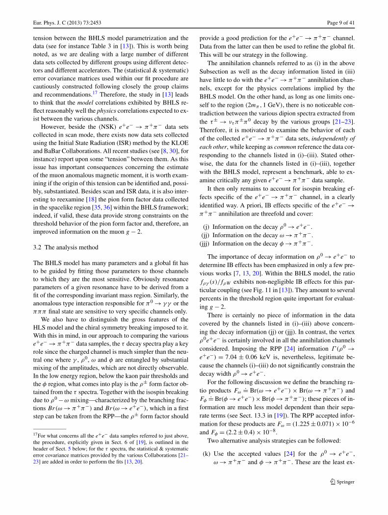
Figure 1(a) displays the prediction for the pion formfactor in the φ region using the HK mass to estimate theφπ−π+ coupling constant with the BaBar data superim-posed (not fitted); it is clear that the prediction is quite rea-sonable up to �0.98 GeV as well as above �1.05 GeV.However, it is clearly unacceptable for the mass region in-between. In contrast, using the φ mass as given in the RPP toextract the φπ−π+ coupling constant from its accepted par-tial width [24] provides the spectrum shown in Fig. 1(b); thisalternate choice is certainly reasonable all along the massregion displayed. Therefore, it is motivated to update ourformer results [13] by performing the change just empha-sized.23 In order to be complete, it is worth mentioning herea fit result obtained by exchanging the PDG/SND φ decayinformation with the BaBar pion form factor data21 in therange (1.0–1.05) GeV. The result, given in Fig. 1(c), showsthat the lineshape of the BaBar pion form factor at the φ

mass can be satisfactorily accommodated. As the exact poleposition of the φ meson is determined by a benchmark in-dependent of the e+e− → π−π+ process (see Sect. 3), thedrop exhibited by Fig. 1(c) in the BaBar is perfectly consis-tent with an expected φ signal.

4 τ predictions of the pion form factor

4.1 τ + PDG predictions

As mentioned before, the charged isovector τ± → ντπ±π0

dipion spectra are not affected by γ −ρ −ω−φ mixing and

22As the HK mass for the ω meson coincides almost exactly with itsaccepted RPP value, the problem actually arises only for the φ meson.23We show later on that choosing the φ HK mass has produced someoverestimate of the prediction for aμ and, thus, some underestimate ofthe discrepancy with the BNL measurement [39, 40].

Eur. Phys. J. C (2013) 73:2453 of 41

Fig. 1 The e+e− → π+π−cross section around the φ masstogether with BaBar datasuperimposed. The curve in (a)displays the prediction using theRPP φ decay informationcomputed at the φ

Higgs–Kibble mass; the curve in(b) displays the prediction usingthe PDG φ decay informationcomputed at the experimental φ

mass. In (c) the PDG φ decayinformation is replaced by thefive BaBar data points locatedbetween 1. and 1.05 GeV

hence are of much simpler structure. Supplemented by thebasic ρ − ω − φ mixing effects which derive from SU(2)

and SU(3) flavor breaking, one has a good starting point tofix the parameters of the BHLS model to predict the pro-cess e+e− → π+π−. Specifically, we are using the dataincluding the channels listed in (i)–(iv) of Sect. 3 togetherwith RPP information relevant to fix the IB effects affect-ing the pion form factor. This method is named, somewhatabusively24 τ + PDG.

Specifically, the IB effects encoded in Br(ω → π+π−),Fω

.= Br(ω → e+e−) × Br(ω → π+π−) and Fφ.= Br(φ →

e+e−) × Br(φ → π+π−) are taken from the RPP. For themissing phase information we adopt the result from the fit[70] for the Orsay phase of the ω → π+π− amplitude andthe result from SND [72] for the phase of the φ → π+π−amplitude.25 Following the discussion in the preceding sub-

24By abusively, we mean, first that the “Orsay” phases for both the ω

and φ mesons have no entry in the RPP and, second, that the bench-mark represented by the processes listed in Sect. 3 within items (i) to(iv) have little to do with τ or the RPP.25A preliminary version of the present work was presented [73] atthe Workshop on Meson Transition Form Factors held on May 29–

section, the model branching ratios and phases are computedat the vector boson masses accepted by the RPP.

The fit returns a probability of 89.4 % with χ2/ndof =553.4/596. The fit quality (χ2/npoints) for each of the fittedchannels is almost identical to our results in [13] (see the lastcolumn in Table 3 therein). Each of the decay partial widthextracted from [24] contributes by �1 to the total χ2. It isalso worth mentioning that the dipion spectra from [21–23]are nicely described up to

√s = 1 GeV and provide residual

distributions indistinguishable from those shown in Fig. 10of [13]. From this fit, one derives the (τ + PDG) predictionsfor the pion form factor which can be compared with thevarious existing e+e− → π+π− data samples.

The overall view of the comparison is shown in Fig. 2.This clearly indicates that the data associated with the chan-nels listed in (i)–(iv), supplemented with a limited PDG in-formation is indeed able to provide already a satisfactory

30, 2012 in Krakow, Poland. Some minor differences may occur withthe present results due to the fact that the SND phase for φ → π+π−was not imposed in the preliminary work.

of 41 Eur. Phys. J. C (2013) 73:2453

Fig. 2 The Pion Form Factorprediction based on τ data andPDG information. The mostimportant experimental data aresuperimposed; they do notinfluence the predicted curve

picture of the pion form factor as reported by all experimentshaving published e+e− → π+π− spectra.

Let us stress that the predicted pion form factor relies onthe π±π0 spectra provided by ALEPH [21], Belle [23] andCLEO [22] only up to 1.0 GeV. Therefore, the inset in Fig. 2actually shows the extrapolation of the prediction into thespacelike region with the NA7 data [35] superimposed; thisclearly indicates that there is no a priori reason to discard thespacelike data from our data handling. One should also notethat the extrapolation of the prediction above the φ mass isquite reasonable up to �1.2–1.3 GeV. This may indicatethat the influence of high mass vector mesons is negligibleup to this energy region.

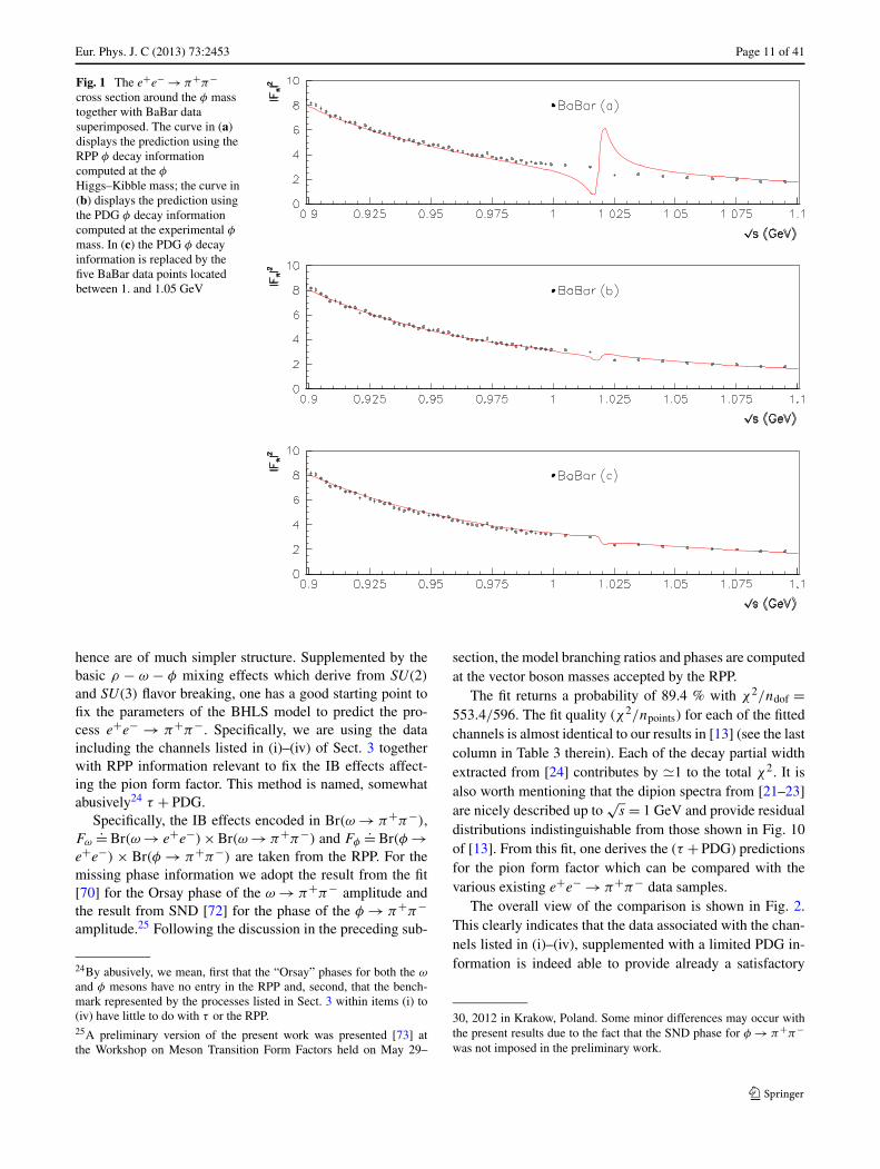
In order to make more precise statements, let us magnifypiece wise the information carried by Fig. 2. Thus, Fig. 3displays the behavior of the various e+e− → π+π− datasamples in the (0.3–0.7) GeV energy region. As a generalstatement the behavior expected from the existing data sam-ples looks well predicted by the τ + PDG method. A closerinspection allows to infer that the CMD-2 and SND datapoints (i.e. NSK when used together) are well spread ontoboth sides of the predicted curve; this property is also shared

by the KLOE10 sample. Even if reasonably well described,the KLOE08 and BaBar data samples are lying slightlyabove the τ +PDG expectations; this difference should van-ish when including the π+π− spectra inside the fit proce-dure.

Figure 4 displays the behavior of the various e+e− →π+π− data samples in the (0.85–1.2) GeV energy region.Here also the predicted curve accounts well for the data be-havior. A closer inspection tells that the sparse NSK dataare well described. The BaBar data are also well accountedfor all along this energy interval except for the φ region. Asshown by Fig. 1(c) above, this can be cured and one canshow that the difference is mostly due to the phase for theφ → π+π− amplitude which departs significantly26 fromthose provided by SND [72]. One could also note that bothKLOE data samples look slightly below the τ +PDG expec-tations in this region.

One may conclude from Figs. 3 and 4 that our “τ +PDG”predictions are in good agreement with the data and that a

26 This issue is examined in detail in Sect. 5.2.1 below.

Eur. Phys. J. C (2013) 73:2453 of 41

Fig. 3 Magnified view of thePion Form Factor predictionbased on τ data and PDGinformation; the (0.3–0.7) GeVregion is shown with theindicated data superimposed

fit using fully these data samples should provide marginaldifferences between all π+π− data sets.27

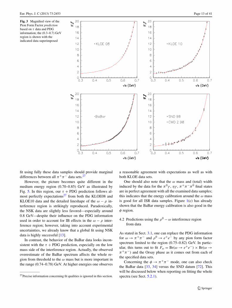
However, the picture becomes quite different in themedium energy region (0.70–0.85) GeV as illustrated byFig. 5. In this region, our τ + PDG prediction follows al-most perfectly expectations27 from both the KLOE08 andKLOE10 data and the detailed lineshape of the ω − ρ in-terference region is strikingly reproduced. Paradoxically,the NSK data are slightly less favored—especially around0.8 GeV—despite their influence on the PDG informationused in order to account for IB effects in the ω − ρ inter-ference region; however, taking into account experimentaluncertainties, we already know that a global fit using NSKdata is highly successful [13].

In contrast, the behavior of the BaBar data looks incon-sistent with the τ + PDG prediction, especially on the lowmass side of the interference region. Actually, the observedoverestimate of the BaBar spectrum affects the whole re-gion from threshold to the ω mass but is more important inthe range (0.74–0.78) GeV. At higher energies one observes

27Precise information concerning fit qualities is ignored in this section.

a reasonable agreement with expectations as well as withboth KLOE data sets.

One should also note that the ω mass and (total) widthinduced by the data for the π0γ , ηγ , π+π−π0 final statesare in perfect agreement with all the examined data samples;this indicates that the energy calibration around the ω massis good for all ISR data samples. Figure 1(c) has alreadyshown that the BaBar energy calibration is also good in theφ region.

4.2 Predictions using the ρ0 − ω interference regionfrom data

As stated in Sect. 3.1, one can replace the PDG informationfor ω → π+π− and ρ0 → e+e− by any pion form factorspectrum limited to the region (0.75–0.82) GeV. In partic-ular, this turns out to fit Fω = Br(ω → e+e−) × Br(ω →π+π−) and the Orsay phase as it comes out from each ofthe specified data sets.

Concerning the φ → π+π− mode, one can also checkthe BaBar data [33, 34] versus the SND datum [72]. Thiswill be discussed below when reporting on fitting the wholespectra (see Sect. 5.2.1).

of 41 Eur. Phys. J. C (2013) 73:2453


Table 1 Fit results for Fω.= Br(ω → e+e−)Br(ω → π+π−) and

for the Orsay phase (in degrees) using only the (0.75–0.82) GeV en-ergy region of each π+π− data sample. The fit is done following the(local) procedure sketched in Sect. 4.2; we use Br(ω → π+π−) =

(1.53 ± 0.13) % [24] and the Orsay phase from [70] as input valuesfor the “τ + PDG” fit. The probabilities are those of the global fit; thelast data column shows the contribution of each π+π− data set to thetotal χ2 and gives the corresponding number of data points

Data Sample Local Fit

Fω 106 Orsay Phase (degrees) Prob. (%) χ2/nπ+π−

Reference values [29, 70] 1.225 ± 0.071 104.70 ± 4.10 – –

τ + PDG 1.157 ± 0.053 108.92 ± 2.36 89.4 % –

τ + NSK [27, 29] 1.219 ± 0.043 106.71 ± 0.25 90.0 % 52/47

τ + KLOE08 [31] 1.076 ± 0.041 110.44 ± 1.24 87.8 % 18/11

τ + KLOE10 [32] 0.973 ± 0.045 113.62 ± 1.63 92.7 % 11/11

τ + BaBar [33] 1.780 ± 0.011 107.50 ± 0.19 54.4 % 67/35

Using the RPP recommended value for Br(ω → π+π−)

and the Orsay phase information from [70] yields a value forFω in good correspondence with expectations, as clear fromthe entry τ + PDG in Table 1. Using NSK data or any ofboth KLOE samples, instead of the PDG information, doesnot lead to predicted curves substantially different from theiranalogue already shown and commented upon in the previ-

ous subsection. Interesting parameter values have been ex-tracted from global fits using only the (0.75–0.82) GeV re-gion from the NSK and KLOE spectra for e+e− → π+π−and are reported in Table 1; they are in reasonable agree-ment with the reported branching ratio product Fω [29] andthe Orsay phase [70, 71] as well. Indeed, taking the RPPFω value as reference, our estimates using the 70 MeV in-

Eur. Phys. J. C (2013) 73:2453 of 41


terval surrounding the interference region are at 0.1σ , 1.8σ

and 3.0σ for respectively the NSK [27, 29], KLOE08 [31]and KLOE10 [32] data samples. The difference between theRPP recommended value for Fω and our entry for NSKalso tells that the BHLS parametrization and the more stan-dard form factor lineshape used by SND [29] provide almostidentical values for Fω.

As far as BaBar data are concerned, the situation looksdifferent and the most relevant piece of information is pro-vided in Fig. 6. This proves that the largest difference be-tween BaBar data and the other analogous data samples [27,29, 31, 32] is the Fω information inherent to the BaBar data.Clearly, Table 1 shows that the BaBar value for Fω is offfrom its recommended value by (7–8)σ . This strong dis-agreement is substantiated by comparing Figs. 5 and 6.

Table 1 also reports the fit probability for each of the ex-amined configurations. With about 90 % probabilities, the“τ + PDG” prediction and the NSK, KLOE08 and KLOE10(global) fits exhibit a full consistency with the rest of ourbenchmark (i.e. all other annihilation channel physics). Theagreement of this with BaBar data, even limited to such atiny interval, is found much poorer and exhibits a clear ten-

sion between F BaBarω and the rest of the (non-π+π−) physics

accessible to the HLS model.Additional pieces of information are provided in the last

data column of Table 1 which complements the global fitprobabilities. These are the values for χ2/nπ+π− for eachof the various π+π− data samples, nπ+π− being the numberof data points included in the fitted energy range (i.e. (0.75–0.82) GeV).

4.3 Isospin breaking effects in the BHLS model: comments

It follows from the developments just above that the BHLSmodel fed with a limited number of accepted values forsome IB pieces of information is indeed able to provide aquite satisfactory prediction for the e+e− → π+π− crosssection once the τ spectra are considered. This gives sup-port to our breaking model, especially to the s-dependentvector meson mixing mechanism.

The prediction is found in accord with the scan (NSK)data samples and with both KLOE data sets.28 Indeed,

28Some issue with the uncertainties of the KLOE08 data sample willbe discussed below.

of 41 Eur. Phys. J. C (2013) 73:2453

Fig. 6 The Pion Form Factorprediction based on τ data andthe (0.76–0.82) GeV region ofthe BaBar spectrum [33]; the(0.7–0.85) GeV region is shownwith the indicated datasuperimposed

the predicted lineshape strikingly follows the central valuesfrom both KLOE data samples; for the scan data, the predic-tion based on PDG information is good but not as good asfor the KLOE data. However, changing the PDG requestedIB information by less than 1σ—as following from a merecomparison of the first and second lines in Table 1—leadsto a perfect description of the NSK spectra over the wholeavailable energy range [13]. In contrast, the RPP branchingfraction product Fω has to be changed by about 7σ in orderto yield a comparable description of the BaBar [33] data.

Basically, our approach is a τ based prediction of π+π−spectra; it relies on the consistency of several differentphysics channels, the τ spectra and on a model of isospinsymmetry breaking (IB). In fine, our breaking model doesnot carry IB parameter values plugged in from start, butyields the numerical IB effects in a data driven mode. It isthus interesting to examine the consequences of this τ (andglobal) based approach on the muon g − 2 estimated value.For this purpose, it is worth stressing that the τ based es-timates given just below—and later—are not computed byintegrating the τ spectra (and adding corrections like in [8,23], for instance), but by integrating the e+e− cross sections

they allow to reconstruct through the global BHLS frame-work.

This is what is shown in Fig. 7. The first line displays theresult derived from the “τ + PDG” fit. The four followinglines are obtained by replacing the ρ and ω IB informationby the 0.76–0.82 GeV region of the quoted data sets. Theline named BNL displays the experimental result [39, 40]and the last line shows the τ based estimate from [8]. Thelast data column in Fig. 7 gives the probability of the corre-sponding fits.

It is clear that all methods used to include IB effectswithin our τ based approach give consistent results, all dis-tant from the BNL measurement at the 4σ level. The associ-ated probabilities indicate the quality of the fits from wherethey are derived.

5 Global fits using the e+e− → π+π− spectra

As in our previous analysis [13], we have performed globalfits using simultaneously all e+e− annihilation data into the

π0γ , ηγ , π+π−π0, K+K−, K0K0

final states, the dipion

Eur. Phys. J. C (2013) 73:2453 of 41

Fig. 7 τ based estimates using a global fit of the BHLS model (seeSect. 4). The first two numbers in each line display resp. the centralvalue and the r.m.s. of aμ = a

expμ − ath

μ . The last two numbers giveresp. the distance to the BNL measurement and the fit probability—

essentially dominated by the non π+π− data. The lower probabilityfound when using the BaBar data, even in the limited energy regioninvolved ([0.76–0.82] GeV), exhibits the tension of this data samplerelative to the rest of the physics considered

spectra collected in the decay of the τ lepton [21–23] andthe decay information listed in Sect. 3.1. We also use theRPP φ decay properties in the (updated) way emphasized inSect. 3.3.

For what concerns the e+e− → π+π− data includedinto the global fit procedure, we have performed fits usingseparately the NSK, KLOE08 and KLOE10 data samples.Global fits have also been performed for the BaBar dipionspectrum restricted to the range of validity of our BHLSmodel. Two options have been considered, using BaBar dataup to 1 GeV supplemented by φ → π+π− decay propertiesfrom the RPP or using the BaBar data up to 1.05 GeV, thusincluding its φ region and avoiding the need of using theRPP information about the φ.

In all cases, the errors (and the χ2) were constructed fol-lowing the information published/recommended by the ex-perimental groups who collected these data. For instance,concerning the scan data samples, the full covariance ma-trix is generally constructed by adding the systematic er-ror covariance matrix Vsyst to the (diagonal) statistical co-variance Vstat constructed from the tabulated uncertaintiesas described in [19] (see Sect. 6 therein); Vsyst is con-structed assuming the reported systematic errors bin-to-bincorrelated.29 Nevertheless, for the rather imprecise e+e− →(π0/η)γ data, taking into account the large magnitude ofthe reported systematics, the systematic and statistical errorswere simply added in quadrature. For the e+e− → π+π−π0

data, we dealt with depending on the level of precision of therelevant data sample (see Sect. 2.2.3 in [20] for more infor-mation).

29When they are reported, uncorrelated systematics are simply addedin quadrature to the statistical errors.

For the τ data, as both Vsyst and Vstat are publicly avail-able [21–23], one only has to add them up, as already per-formed for the study in [13]. For the BaBar sample, the sys-tematic uncertainties on the cross section are given (as afunction of

√s) in Table V from [34] and are imposed to

be 100 % bin-to-bin correlated (following Sect. F in [34]).Writing, for definiteness, each of these uncertainty functionsas f (si), for the data point mi located at

√si , the (i, j) en-

try of the Vsyst matrix is given by the sum of the variousf (si)f (sj )mimj .

For both the KLOE08 and KLOE10 data samples[31, 32], the KLOE Collaboration provides basically thesame information as BaBar and therefore, we simply haveto proceed likewise.

Moreover, the various π+π− data sets collected byCMD-2 and SND [27–29] on the one hand and the olderdata samples from [25] on the other hand, both carry com-mon bin-to-bin and sample-to-sample correlated uncertain-ties estimated resp. to 0.4 % and �1 %. As in our previousstudies [13, 20], this effect is accounted for in the minimiza-tion code. These are the most important reported correla-tions of this type within the scan data [74].

We have also performed global fits using combinations ofthese individual π+π− data samples. In this case, the con-tributions of the NSK and KLOE10 data to the total χ2 wereleft unweighted as their own χ2/n contribution is always ofthe order 1 in fits using each of them in “isolation”.30 In con-trast, in such combinations involving the KLOE08 and/or

30We remind that, in this work, the wording “isolation” or “stan-dalone” is always used to qualify the fits performed using a specifice+e− → π+π− data sample. It is understood that each of the π+π−data sets “fitted in isolation” is always fitted in conjunction with all theother data listed in Sect. 3.1. When several of the e+e− → π+π− datasamples are submitted to fit (together with the other channels), we then

of 41 Eur. Phys. J. C (2013) 73:2453

BaBar data, the contribution of each of these to the total χ2

was weighted by the ratio fM = nM/χ2M (M = KLOE08,

BaBar) where χ2M is the χ2 of the M data set obtained in the

best fit using only M as e+e− → π+π− data set; nM is thecorresponding number of data points. In fits involving thespacelike data [35, 36], the corresponding weight was alsoused.31

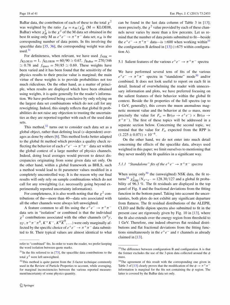
For definiteness, when relevant, we have used fNSK =fKLOE10 = 1, fKLOE08 = 60/90 � 0.67, fBaBar = 270/346� 0.78 and fspace = 59/85 � 0.69. These weights havebeen varied and it has been found that the sensitivity of thephysics results to their precise value is marginal; the mainvirtue of these weights is to provide probabilities not toomuch ridiculous. On the other hand, as a matter of princi-ple, when results are displayed which have been obtainedusing weights, it is quite generally for the reader’s informa-tion. We have preferred being conclusive by only relying onthe largest data set combinations which do not call for anyreweighting. Indeed, this simply reflects that global fit prob-abilities do not raise any objection to trusting the uncertain-ties as they are reported together with each of the used datasets.

This method,32 turns out to consider each data set as aglobal object, rather than defining local (s-dependent) aver-ages as done by others [6]. This method looks better adaptedto the global fit method which provides a quality check re-flecting the behavior of each e+e− → π+π− data set withinthe global context of a large number of physics channels.Indeed, doing local averages would prevent to detect dis-crepancies originating from some given data set only. Onthe other hand, within a global framework as BHLS, sucha method would lead to fit parameter values modified in acompletely uncontrolled way. It is the reason why our finalresults will only rely on sample combinations which do notcall for any reweighting (i.e. necessarily going beyond ex-perimentally reported uncertainty information).

For completeness, it is also worth noting that the χ2 con-tributions of the—more than 40—data sets associated withall the other channels were always left unweighted.

A feature common to all fits using the e+e− → π+π−data sets in “isolation” or combined is that the individualχ2 contributions associated with the other channels (π0γ ,

ηγ , π+π−π0, K+K−, K0K0, . . .) were only marginally af-

fected by the specific choice of e+e− → π+π− data submit-ted to fit. Their typical values are almost identical to what

refer to “combined” fits. In order to warn the reader, we prefer keepingthe word isolation between quote marks.31In the fits referred to in [73], the spacelike data contributions to thetotal χ2 were left unweighted.32This method is quite parent from the S-factor technique commonlyused in the Review of Particle Properties to account, while averaging,for marginal inconsistencies between the various reported measure-ment/uncertainty of some physics quantity.

can be found in the last data column of Table 3 in [13];more precisely, the χ2 value provided by each of these chan-nels never varies by more than a few percents. Let us re-mind that the number of data points submitted to fit—besidethe e+e− → π+π− data—is �600 when working within33

the configuration B defined in [13] (�675 within configura-tion A).

5.1 Salient features of the various e+e− → π+π− spectra

We have performed several tens of fits of the variouse+e− → π+π− spectra in “standalone” mode30 and/orcombined. It does not look useful to report on each fit indetail. Instead of overwhelming the reader with unneces-sary information and plots, we have preferred focusing onthe salient features of their behavior within the global fitcontext. Beside the fit properties of the full spectra (up to1 GeV, generally), this covers the muon anomalous mag-netic moment value and the behavior at the ω mass, moreprecisely the value for Fω = Br(ω → e+e−) × Br(ω →π+π−). The first of these topics will be addressed in aseparate section below. Concerning the second topic, weremind that the value for Fω expected from the RPP is(1.225 ± 0.071) × 10−6.

On the other hand, we do not enter into much detailconcerning the effects of the spacelike data, always usedweighted in this paper; we limit ourselves to mentioning thatthey never modify the fit qualities in a significant way.

5.1.1 “Standalone” fits of the e+e− → π+π− spectra

When using only30 the (unweighted) NSK data, the fit re-turns34 χ2

NSK/Nπ+π− = 128.30/127 and a global fit proba-bility of 96.3 %. The fit residuals are displayed in the toppanel of Fig. 8 and the fractional deviations from the fittingfunction in the bottom panel. Taking into account the uncer-tainties, both plots do not exhibit any significant departurefrom flatness. The fit residual distributions of the ALEPH,CLEO and Belle dipion spectra also submitted to fit in thepresent case are rigorously given by Fig. 10 in [13], wherethe fit also extends over the energy region from threshold to1 GeV. Therefore, one indeed observes flat residual distri-butions and flat fractional deviations from the fitting func-tions simultaneously in the e+e− and τ channels as alreadyclaimed in [13].

33The difference between configuration B and configuration A is thatthe former excludes the use of the 3-pion data collected around the φ

mass.34The agreement of this result with the corresponding one given inTable 3 of [13] clearly proves that the modification of the φ → π+π−information is marginal for the fits not containing the φ region. Thelatter is covered by the BaBar data set only.

Eur. Phys. J. C (2013) 73:2453 of 41

Fig. 8 Fit residuals for theCMD-2 and SND data samples(NSK) in isolation.30 The toppanel shows the functionδ|Fπ(s)|2 = |F NSK

π (s)|2 −|F fit

π (s)|2; the bottom paneldisplays the distributionδ|Fπ(s)|2/|F fit

π (s)|2

Similarly, the KLOE10 data set [32] returns χ2KLOE10/

Nπ+π− = 73.68/75 and a global fit probability of 87.7 %.The fit residual distribution is shown in the top panel ofFig. 9; the bottom panel in this Figure shows the fractionaldeviations from the fitting function. Both distributions canbe considered as reasonably flat. As in the above Fig. 8, theplotted errors are the square roots of the diagonal elementsof the (full) error covariance matrix. Therefore, the valuefor χ2

KLOE10 and the flatness of the residuals shown in Fig. 9illustrate that the (reported in [32]) full error covariance ma-trix looks correctly understood.

Therefore, within the global fit context, each of the NSKand KLOE10 data samples exhibits the same outstandingbehavior.35 On the other hand, the fit parameters and er-ror covariance matrix allows to derive, using obvious no-tations, F NSK

ω = (1.205 ± 0.042) × 10−6 close to the PDG

35As emphasized in our previous works [13, 19, 20], the global proba-bilities are enhanced thanks to the highly favorable fit properties of thee+e− → (π0/η)γ data; indeed, χ2/N for these are respectively �0.76and 0.66.

value reported at top of Table 1. One also gets F KLOE10ω =

(1.074±0.051)×10−6, a �2.5σ difference with the centralvalue for F NSK

ω .Under the same conditions, the (unweighted) KLOE08

data set returns χ2KLOE08/Nπ+π− = 96.55/60 and a global

fit probability of 56 %, which is rather low. It is worth not-ing the remarkable flatness of the residual distributions dis-played by Fig. 10 which does not prevent to yield a relativelylarge value for χ2

KLOE08. The large χ2KLOE08 and the flatness

of the residual distribution shown in Fig. 10, considered to-gether, might indicate an issue with the non-diagonal part ofthe full error covariance matrix. Anyway, one can concludethat the poor KLOE08 fit probability reflects an issue withthe KLOE08 error estimate rather than a distorted lineshape.

Figure 10 should be compared with the similar distribu-tion derived formerly using a primitive version of the BHLSmodel (see Fig. 3 in [19]). The clear improvement substan-tiates the gain provided by the BHLS model in its presentform. On the other hand, one should also note that the valuefor F KLOE08

ω = (1.117 ± 0.042) × 10−6 is consistent withF KLOE10

ω .

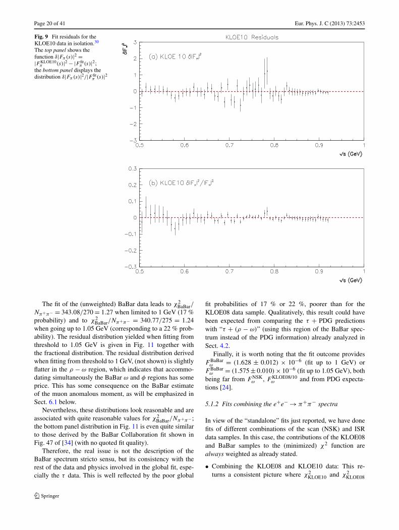
of 41 Eur. Phys. J. C (2013) 73:2453

Fig. 9 Fit residuals for theKLOE10 data in isolation.30

The top panel shows thefunction δ|Fπ(s)|2 =|F KLOE10

π (s)|2 − |F fitπ (s)|2;

the bottom panel displays thedistribution δ|Fπ(s)|2/|F fit

π (s)|2

The fit of the (unweighted) BaBar data leads to χ2BaBar/

Nπ+π− = 343.08/270 = 1.27 when limited to 1 GeV (17 %probability) and to χ2

BaBar/Nπ+π− = 340.77/275 = 1.24when going up to 1.05 GeV (corresponding to a 22 % prob-ability). The residual distribution yielded when fitting fromthreshold to 1.05 GeV is given in Fig. 11 together withthe fractional distribution. The residual distribution derivedwhen fitting from threshold to 1 GeV, (not shown) is slightlyflatter in the ρ − ω region, which indicates that accommo-dating simultaneously the BaBar ω and φ regions has someprice. This has some consequence on the BaBar estimateof the muon anomalous moment, as will be emphasized inSect. 6.1 below.

Nevertheless, these distributions look reasonable and areassociated with quite reasonable values for χ2

BaBar/Nπ+π− ;the bottom panel distribution in Fig. 11 is even quite similarto those derived by the BaBar Collaboration fit shown inFig. 47 of [34] (with no quoted fit quality).

Therefore, the real issue is not the description of theBaBar spectrum stricto sensu, but its consistency with therest of the data and physics involved in the global fit, espe-cially the τ data. This is well reflected by the poor global

fit probabilities of 17 % or 22 %, poorer than for theKLOE08 data sample. Qualitatively, this result could havebeen expected from comparing the τ + PDG predictionswith “τ + (ρ − ω)” (using this region of the BaBar spec-trum instead of the PDG information) already analyzed inSect. 4.2.

Finally, it is worth noting that the fit outcome providesF BaBar

ω = (1.628 ± 0.012) × 10−6 (fit up to 1 GeV) orF BaBar

ω = (1.575 ± 0.010) × 10−6 (fit up to 1.05 GeV), bothbeing far from F NSK

ω , F KLOE08/10ω and from PDG expecta-

tions [24].

5.1.2 Fits combining the e+e− → π+π− spectra

In view of the “standalone” fits just reported, we have donefits of different combinations of the scan (NSK) and ISRdata samples. In this case, the contributions of the KLOE08and BaBar samples to the (minimized) χ2 function arealways weighted as already stated.

• Combining the KLOE08 and KLOE10 data: This re-turns a consistent picture where χ2

KLOE10 and χ2KLOE08

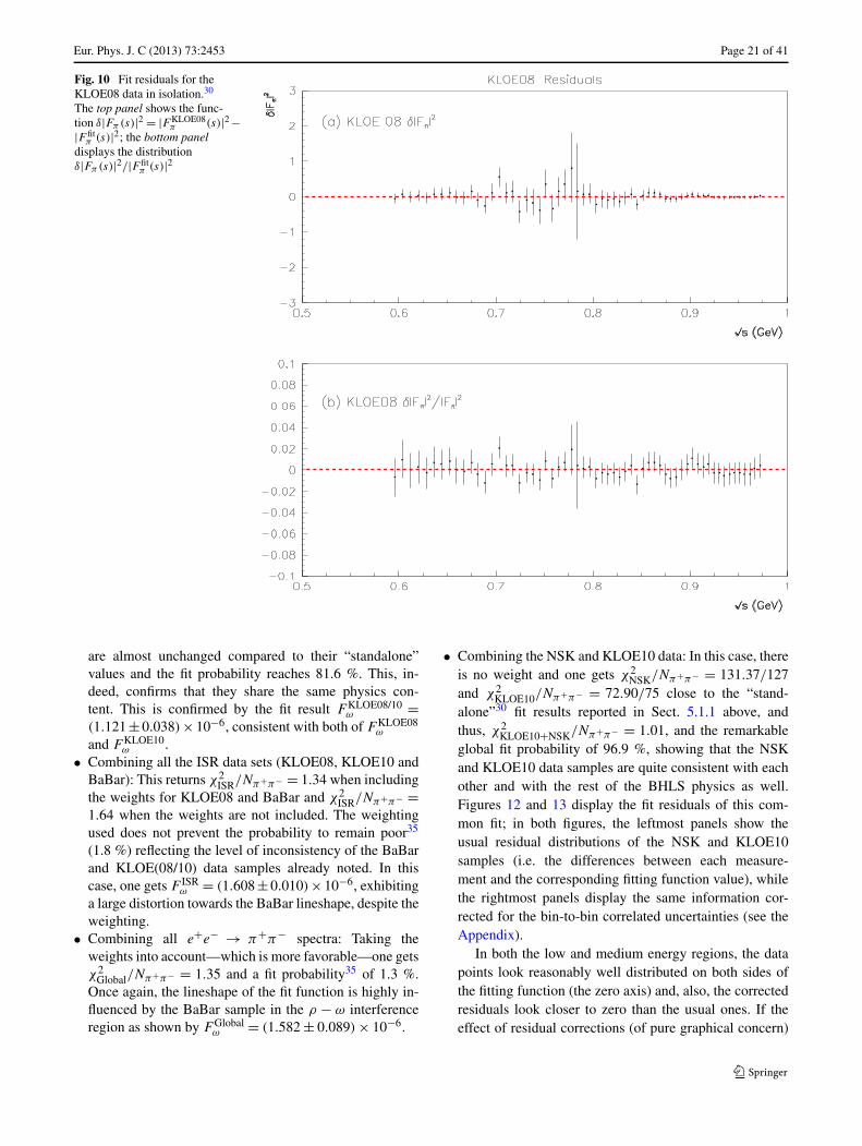
Eur. Phys. J. C (2013) 73:2453 of 41

Fig. 10 Fit residuals for theKLOE08 data in isolation.30

The top panel shows the func-tion δ|Fπ(s)|2 = |F KLOE08

π (s)|2 −|F fit


π (s)|2

are almost unchanged compared to their “standalone”values and the fit probability reaches 81.6 %. This, in-deed, confirms that they share the same physics con-tent. This is confirmed by the fit result F KLOE08/10

ω =(1.121 ± 0.038)× 10−6, consistent with both of F KLOE08

ω

and F KLOE10ω .

• Combining all the ISR data sets (KLOE08, KLOE10 andBaBar): This returns χ2

ISR/Nπ+π− = 1.34 when includingthe weights for KLOE08 and BaBar and χ2

ISR/Nπ+π− =1.64 when the weights are not included. The weightingused does not prevent the probability to remain poor35

(1.8 %) reflecting the level of inconsistency of the BaBarand KLOE(08/10) data samples already noted. In thiscase, one gets F ISR

ω = (1.608 ± 0.010)× 10−6, exhibitinga large distortion towards the BaBar lineshape, despite theweighting.

• Combining all e+e− → π+π− spectra: Taking theweights into account—which is more favorable—one getsχ2

Global/Nπ+π− = 1.35 and a fit probability35 of 1.3 %.Once again, the lineshape of the fit function is highly in-fluenced by the BaBar sample in the ρ − ω interferenceregion as shown by F Global

ω = (1.582 ± 0.089) × 10−6.

• Combining the NSK and KLOE10 data: In this case, thereis no weight and one gets χ2

NSK/Nπ+π− = 131.37/127and χ2

KLOE10/Nπ+π− = 72.90/75 close to the “stand-alone”30 fit results reported in Sect. 5.1.1 above, andthus, χ2

KLOE10+NSK/Nπ+π− = 1.01, and the remarkableglobal fit probability of 96.9 %, showing that the NSKand KLOE10 data samples are quite consistent with eachother and with the rest of the BHLS physics as well.Figures 12 and 13 display the fit residuals of this com-mon fit; in both figures, the leftmost panels show theusual residual distributions of the NSK and KLOE10samples (i.e. the differences between each measure-ment and the corresponding fitting function value), whilethe rightmost panels display the same information cor-rected for the bin-to-bin correlated uncertainties (see theAppendix).

In both the low and medium energy regions, the datapoints look reasonably well distributed on both sides ofthe fitting function (the zero axis) and, also, the correctedresiduals look closer to zero than the usual ones. If theeffect of residual corrections (of pure graphical concern)

of 41 Eur. Phys. J. C (2013) 73:2453

Fig. 11 Fit residuals for theBaBar data sample in isolation30

over the energy range fromthreshold to 1.05 GeV. The toppanel shows the functionδ|Fπ(s)|2 = |F BaBar

π (s)|2 −|F fit


π (s)|2. Thevertical dashed lines indicatethe upper end of the fittedspectrum

looks marginal at low to medium energies, the rightmostpanel of Fig. 13 clearly indicates the more appropriatecharacter of the corrected residuals to translate the fitquality.

As the global fit including simultaneously the CMD-2 [26–28], SND [29] and KLOE10 [32] π+π− datasets play a crucial role in the present study, it looksworth to give more information on their fit quality be-yond the global properties just emphasized. This is thepurpose of Table 2. We choose here to present the re-sults in terms of probabilities of the χ2

π+π− contribu-tions to the total χ2 associated with the correspond-ing number of data points36 Nπ+π− . The last data col-umn thus gives this probability for the data sample(s)provided by the three experiments. From this exerciseone can conclude that the three data samples, eachas a whole, behave normally with a remarkable fitquality of the SND data sample (χ2/Npoints � 0.7),

36This does not correspond to numbers of degrees of freedom, impos-sible to define in this circumstance.

while KLOE10 (χ2/Npoints � 1.0) and the (collection)of CMD-2 (χ2/Npoints � 1.1) data samples are quite rea-sonable.

Even if more approximate, one can perform the sameexercise for various energy subregions.37 This is dis-played in the first four data columns of Table 2. The prob-abilities of the various SND data subsamples (Nπ+π− =45) look reasonably flat, pointing to a very good accountby the model function and one yields χ2/Npoints’s rang-ing between 0.5 and 1.1. The probabilities of the CMD2collection of data subsamples (Nπ+π− = 82) are lessfavorable (the χ2/Npoints’s range between 0.7 and 1.3)but remain quite acceptable. The results for KLOE10(Nπ+π− = 75) is more appealing as the probabilitiesare good for three regions (corresponding to χ2/Npoints

values of resp. 0.3, 1.2 and 0.5), while the fourth re-gion is much worse (1.7 % probability corresponding to

37In this case, the notion of partial χ2 should be handled with somecare as the number of data points is small in several bins and the inter–region correlations are neglected.

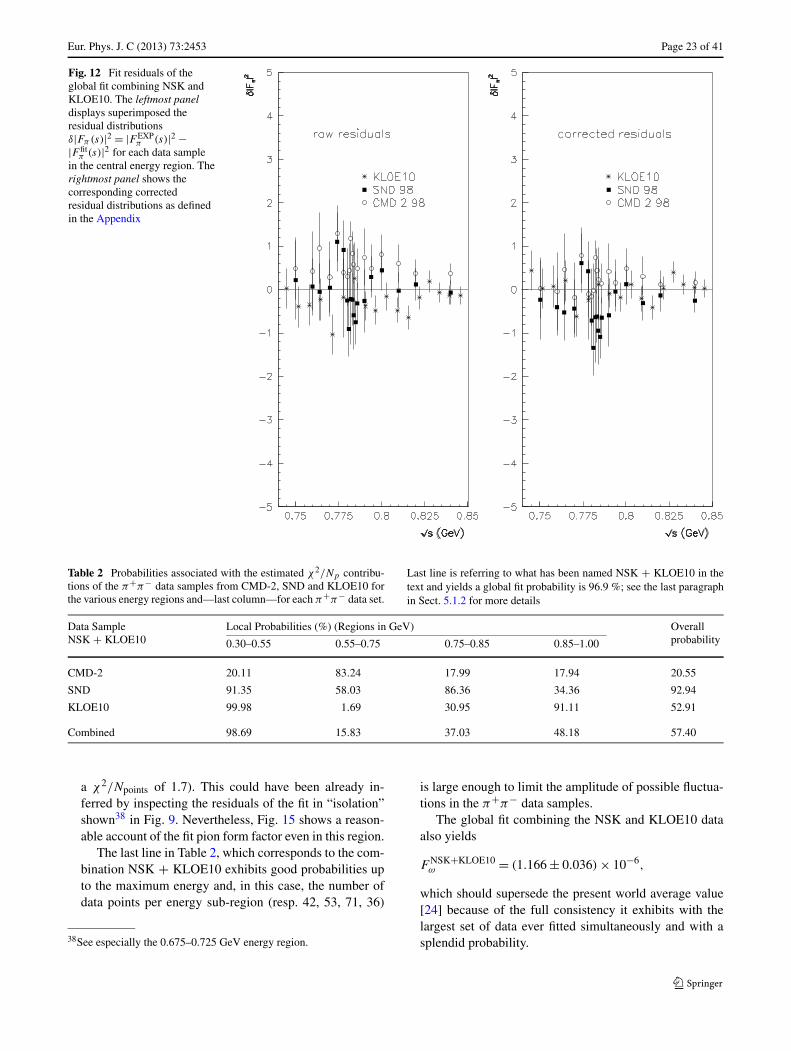
Eur. Phys. J. C (2013) 73:2453 of 41

Fig. 12 Fit residuals of theglobal fit combining NSK andKLOE10. The leftmost paneldisplays superimposed theresidual distributionsδ|Fπ(s)|2 = |F EXP

π (s)|2 −|F fit

π (s)|2 for each data samplein the central energy region. Therightmost panel shows thecorresponding correctedresidual distributions as definedin the Appendix

Table 2 Probabilities associated with the estimated χ2/Np contribu-tions of the π+π− data samples from CMD-2, SND and KLOE10 forthe various energy regions and—last column—for each π+π− data set.

Last line is referring to what has been named NSK + KLOE10 in thetext and yields a global fit probability is 96.9 %; see the last paragraphin Sect. 5.1.2 for more details

Data SampleNSK + KLOE10

Local Probabilities (%) (Regions in GeV) Overallprobability0.30–0.55 0.55–0.75 0.75–0.85 0.85–1.00

CMD-2 20.11 83.24 17.99 17.94 20.55

SND 91.35 58.03 86.36 34.36 92.94

KLOE10 99.98 1.69 30.95 91.11 52.91

Combined 98.69 15.83 37.03 48.18 57.40

a χ2/Npoints of 1.7). This could have been already in-ferred by inspecting the residuals of the fit in “isolation”shown38 in Fig. 9. Nevertheless, Fig. 15 shows a reason-able account of the fit pion form factor even in this region.

The last line in Table 2, which corresponds to the com-bination NSK + KLOE10 exhibits good probabilities upto the maximum energy and, in this case, the number ofdata points per energy sub-region (resp. 42, 53, 71, 36)

38See especially the 0.675–0.725 GeV energy region.

is large enough to limit the amplitude of possible fluctua-tions in the π+π− data samples.

The global fit combining the NSK and KLOE10 dataalso yields

F NSK+KLOE10ω = (1.166 ± 0.036) × 10−6,

which should supersede the present world average value[24] because of the full consistency it exhibits with thelargest set of data ever fitted simultaneously and with asplendid probability.

of 41 Eur. Phys. J. C (2013) 73:2453

Fig. 13 Fit residuals of theglobal fit combining NSK andKLOE10. The leftmost panelsdisplay (superimposed) theresidual distributionsδ|Fπ(s)|2 = |F EXP

π (s)|2 −|F fit

π (s)|2 for each data samplein the side energy regions. Therightmost panels show thecorresponding correctedresidual distributions as definedin the Appendix

5.1.3 Fits of the e+e− → π+π− spectra:concluding remarks

The results reported just above have allowed us to showthat the NSK data are in fair agreement with the physics

represented by the π0γ , ηγ , π+π−π0, K+K−, K0K0

an-nihilation channels, the dipion spectra collected in the de-cay of the τ lepton and some more decay information listedin Sect. 3.1. This is not a really new result as this conclu-sion was already reached in our previous analysis [13]. Thesingle difference with [13] is the new way to include theφ → π+π− information (see Sect. 3.3), possible with theBaBar data.

The new information is that the KLOE10 data samplebehaves likewise and, more importantly, that the NSK andKLOE10 data sets are consistent with each other as wellas with the rest of the physics considered within the BHLSmodel and the global fit context.

We have performed global fits which have shown thatthe data from KLOE08 and BaBar have some difficultyto accommodate the global fit context. For what concernsKLOE08, the problem appears to be related with (underes-

timated?) systematic errors or, possibly, with their correla-tions. In the case of BaBar data, the problem looks moreserious, as it deals with the form factor lineshape itself inthe ρ − ω interference region; this issue manifests itself inthe value for Fω, much larger than expected.

For this purpose, it is interesting to see the behavior ofthe most relevant fits of the pion form factor in the ρ − ω

resonance region. These are displayed in Fig. 14. The bestfit obtained using only the NSK data is shown in the topleft panel and is clearly quite satisfactory. The top rightpanel exhibits the case when the NSK data are comple-mented with the KLOE10 sample; this fit is also quite suc-cessful.

Bottom left panel in Fig. 14 shows the behavior ofthe best fit function when only considering the ISR data(BaBar, KLOE08, KLOE10) and bottom right panel whentaking into account all existing scan and ISR data. Bothare clearly less satisfactory reflecting mostly the tension be-tween BaBar and the KLOE data sets.

As already stated, the largest favored configuration isto include simultaneously the NSK and KLOE10 sampleswithin the fit procedure. Figure 15 shows the fractional de-

Eur. Phys. J. C (2013) 73:2453 of 41

Fig. 14 The Pion Form Factorin the ρ − ω region from variousglobal fit configurations. Top leftpanel displays the best fit usingonly the CMD-2 and SND dataas e+e− → π+π− spectra. Topright panel shows the case whenthe CMD-2, SND and KLOE10data samples are fittedsimultaneously. Bottom leftpanel shows the best fits whenthe data samples considered arethose from BaBar, KLOE08 andKLOE10. Bottom right panelshows the best fit usingsimultaneously the CMD-2,SND, KLOE08, KLOE10 andBaBar data samples

viations from the fitting functions for the e+e− and τ dataderived simultaneously from the global fit. The top panel isclearly consistent with a flat distribution. The bottom panelshows that CLEO and Belle distributions are flat, but alsothat ALEPH data may show a slight s-dependence startingaround 0.8 GeV (quite similar to the top panel in Fig. 55from [34] or to Fig. 12 in [23]). This is a pure consequenceof having introduced the KLOE10 data sample.39

One may thus consider that the statistically favored con-figurations (the so-called NSK and NSK + KLOE10 globalfit configurations) exhibit flat residual distributions simulta-neously in e+e− and τ ππ channels.

The question is now whether the KLOE08 and BaBardata samples can nevertheless help to improve some physicsinformation of important concern as the muon g − 2. Thiswill be discussed in the forthcoming section. Anyway, theKLOE10 data sample already allows to confirm the resultsalready derived using the NSK data and, even, helps in get-ting improved results.

39Compare bottom panels in the present Fig. 15 and in Fig. 10 in [13].

5.2 Physics information derived from global fits

5.2.1 The φ region in the e+e− → π+π− spectrum

Up to now, the φ pieces of information used in our fits/predictions are the RPP value for the product Fφ = Br(φ →e+e−)Br(φ → π+π−) = (2.2 ± 0.4) × 10−8 and the “Or-say” phase for the φ → π+π− amplitude provided by SND[72], namely −34.0 ± 4.0 degrees. In order to avoid over in-terpreting the SND phase as an Orsay phase (i.e. identifiedwith the phase of the product Fe

ωφ(s) gφππ (s) in Eq. (14)

at s = m2φ), we have found worth revisiting this assumption.

Using the NSK and KLOE10 data sets as reference π+π−data sample, we have performed several global fits withinthe BHLS framework.

For definiteness, and for an easy comparison, the first linein Table 3 displays the values extracted from [24, 72] andused in all fits referred to up to now. The second line in thisTable displays the corresponding values reconstructed usingthe final parameter values from the appropriate global fit.The goodness of fit (94.5 % probability) is reflected by theχ2 values shown in the last two data columns. The recon-structed value for Fφ is in very good accord with the (input)

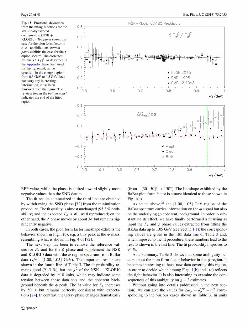
of 41 Eur. Phys. J. C (2013) 73:2453

Fig. 15 Fractional deviationsfrom the fitting functions for thestatistically favoredconfiguration (NSK +KLOE10). Top panel shows thecase for the pion form factor ine+e− annihilations, bottompanel exhibits the case for the τ

dipion spectra. The correctedresiduals δ|Fπ |2, as described inthe Appendix, have been usedfor the top panel; as thespectrum in the energy regionfrom 0.3 GeV to 0.5 GeV doesnot carry any interestinginformation, it has beenremoved from the figure. Thevertical line in the bottom panelindicates the end of the fittedregion

RPP value, while the phase is shifted toward slightly morenegative values than the SND datum.

The fit results summarized in the third line are obtainedby withdrawing the SND phase [72] from the minimizationprocedure. The fit quality is almost unchanged (95.3 % prob-ability) and the expected Fφ is still well reproduced; on theother hand, the φ phase moves by about 3σ but remains sig-nificantly negative.

In both cases, the pion form factor lineshape exhibits thebehavior shown in Fig. 1(b), e.g. a tiny peak at the φ mass,resembling what is shown in Fig. 4 of [72].

The next step has been to remove the reference val-ues for Fφ and for the φ phase and supplement the NSKand KLOE10 data with the φ region spectrum from BaBardata (

√s ∈ [1.00,1.05] GeV). The important results are

shown in the fourth line of Table 3. The fit probability re-mains good (91.3 %), but the χ2 of the NSK + KLOE10data is degraded by �10 units, which may indicate sometension between these data sets and the coherent back-ground beneath the φ peak. The fit value for Fφ increasesby 50 % but remains perfectly consistent with expecta-tions [24]. In contrast, the Orsay phase changes dramatically

(from −[30−50]◦ → 150◦). The lineshape exhibited by theBaBar pion form factor is almost identical to those shown inFig. 1(c).

As stated above,21 the [1.00,1.05] GeV region of theBaBar spectrum carries information on the φ signal but alsoon the underlying (ρ coherent) background. In order to sub-stantiate its effect, we have finally performed a fit using asinput the Fφ and φ phase values extracted from fitting theBaBar data up to 1.05 GeV (see Sect. 5.1.1); the correspond-ing values are given in the fifth data line of Table 3 and,when imposed to the fit procedure, these numbers lead to theresults shown in the last line. The fit probability improves to94 %.

As a summary, Table 3 shows that some ambiguity oc-curs about the pion form factor behavior in the φ region. Itbecomes interesting to have new data covering this region,in order to decide which among Figs. 1(b) and 1(c) reflectsthe right behavior. It is also interesting to examine the con-sequences of this ambiguity on g − 2 estimates.

Without going into details (addressed in the next sec-tion), we can give the values for aμ = a

expμ − ath

μ corre-sponding to the various cases shown in Table 3. In units

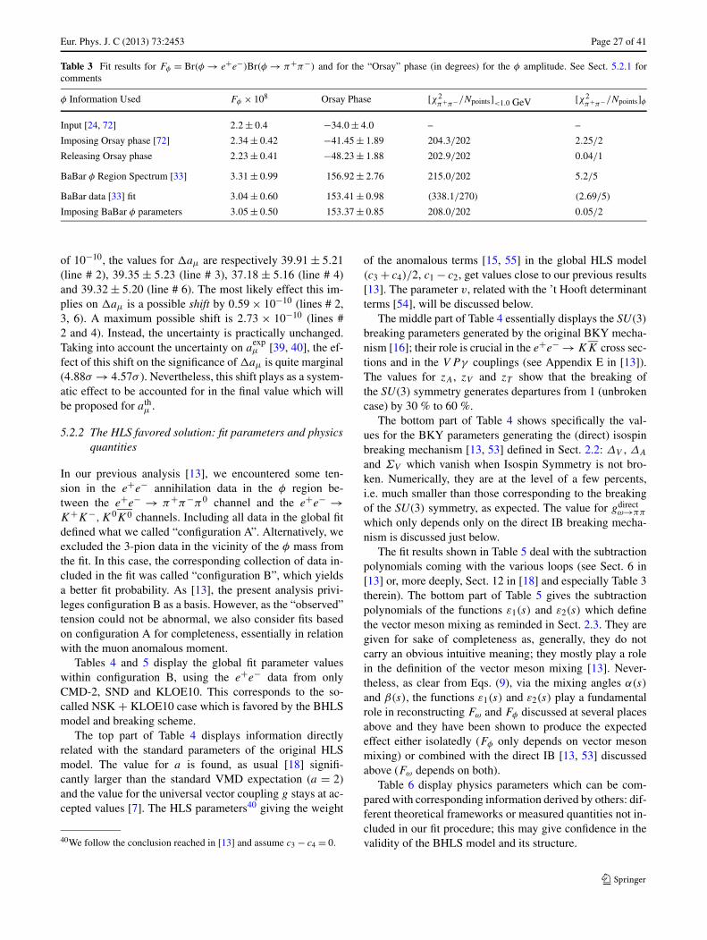
Eur. Phys. J. C (2013) 73:2453 of 41

Table 3 Fit results for Fφ = Br(φ → e+e−)Br(φ → π+π−) and for the “Orsay” phase (in degrees) for the φ amplitude. See Sect. 5.2.1 forcomments

φ Information Used Fφ × 108 Orsay Phase [χ2π+π−/Npoints]<1.0 GeV [χ2

π+π−/Npoints]φ

Input [24, 72] 2.2 ± 0.4 −34.0 ± 4.0 – –

Imposing Orsay phase [72] 2.34 ± 0.42 −41.45 ± 1.89 204.3/202 2.25/2

Releasing Orsay phase 2.23 ± 0.41 −48.23 ± 1.88 202.9/202 0.04/1

BaBar φ Region Spectrum [33] 3.31 ± 0.99 156.92 ± 2.76 215.0/202 5.2/5

BaBar data [33] fit 3.04 ± 0.60 153.41 ± 0.98 (338.1/270) (2.69/5)

Imposing BaBar φ parameters 3.05 ± 0.50 153.37 ± 0.85 208.0/202 0.05/2

of 10−10, the values for aμ are respectively 39.91 ± 5.21(line # 2), 39.35 ± 5.23 (line # 3), 37.18 ± 5.16 (line # 4)and 39.32 ± 5.20 (line # 6). The most likely effect this im-plies on aμ is a possible shift by 0.59 × 10−10 (lines # 2,3, 6). A maximum possible shift is 2.73 × 10−10 (lines #2 and 4). Instead, the uncertainty is practically unchanged.Taking into account the uncertainty on a

expμ [39, 40], the ef-

fect of this shift on the significance of aμ is quite marginal(4.88σ → 4.57σ ). Nevertheless, this shift plays as a system-atic effect to be accounted for in the final value which willbe proposed for ath

μ .

5.2.2 The HLS favored solution: fit parameters and physicsquantities

In our previous analysis [13], we encountered some ten-sion in the e+e− annihilation data in the φ region be-tween the e+e− → π+π−π0 channel and the e+e− →K+K−,K0K0 channels. Including all data in the global fitdefined what we called “configuration A”. Alternatively, weexcluded the 3-pion data in the vicinity of the φ mass fromthe fit. In this case, the corresponding collection of data in-cluded in the fit was called “configuration B”, which yieldsa better fit probability. As [13], the present analysis privi-leges configuration B as a basis. However, as the “observed”tension could not be abnormal, we also consider fits basedon configuration A for completeness, essentially in relationwith the muon anomalous moment.

Tables 4 and 5 display the global fit parameter valueswithin configuration B, using the e+e− data from onlyCMD-2, SND and KLOE10. This corresponds to the so-called NSK + KLOE10 case which is favored by the BHLSmodel and breaking scheme.

The top part of Table 4 displays information directlyrelated with the standard parameters of the original HLSmodel. The value for a is found, as usual [18] signifi-cantly larger than the standard VMD expectation (a = 2)and the value for the universal vector coupling g stays at ac-cepted values [7]. The HLS parameters40 giving the weight

40We follow the conclusion reached in [13] and assume c3 − c4 = 0.

of the anomalous terms [15, 55] in the global HLS model(c3 + c4)/2, c1 − c2, get values close to our previous results[13]. The parameter v, related with the ’t Hooft determinantterms [54], will be discussed below.

The middle part of Table 4 essentially displays the SU(3)

breaking parameters generated by the original BKY mecha-nism [16]; their role is crucial in the e+e− → KK cross sec-tions and in the V Pγ couplings (see Appendix E in [13]).The values for zA, zV and zT show that the breaking ofthe SU(3) symmetry generates departures from 1 (unbrokencase) by 30 % to 60 %.

The bottom part of Table 4 shows specifically the val-ues for the BKY parameters generating the (direct) isospinbreaking mechanism [13, 53] defined in Sect. 2.2: ΔV , ΔA

and ΣV which vanish when Isospin Symmetry is not bro-ken. Numerically, they are at the level of a few percents,i.e. much smaller than those corresponding to the breakingof the SU(3) symmetry, as expected. The value for gdirect

ω→ππ

which only depends only on the direct IB breaking mecha-nism is discussed just below.

The fit results shown in Table 5 deal with the subtractionpolynomials coming with the various loops (see Sect. 6 in[13] or, more deeply, Sect. 12 in [18] and especially Table 3therein). The bottom part of Table 5 gives the subtractionpolynomials of the functions ε1(s) and ε2(s) which definethe vector meson mixing as reminded in Sect. 2.3. They aregiven for sake of completeness as, generally, they do notcarry an obvious intuitive meaning; they mostly play a rolein the definition of the vector meson mixing [13]. Never-theless, as clear from Eqs. (9), via the mixing angles α(s)

and β(s), the functions ε1(s) and ε2(s) play a fundamentalrole in reconstructing Fω and Fφ discussed at several placesabove and they have been shown to produce the expectedeffect either isolatedly (Fφ only depends on vector mesonmixing) or combined with the direct IB [13, 53] discussedabove (Fω depends on both).

Table 6 display physics parameters which can be com-pared with corresponding information derived by others: dif-ferent theoretical frameworks or measured quantities not in-cluded in our fit procedure; this may give confidence in thevalidity of the BHLS model and its structure.

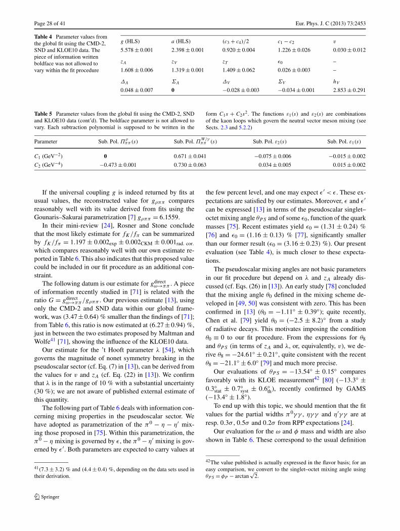
of 41 Eur. Phys. J. C (2013) 73:2453

Table 4 Parameter values fromthe global fit using the CMD-2,SND and KLOE10 data. Thepiece of information writtenboldface was not allowed tovary within the fit procedure

g (HLS) a (HLS) (c3 + c4)/2 c1 − c2 v

5.578 ± 0.001 2.398 ± 0.001 0.920 ± 0.004 1.226 ± 0.026 0.030 ± 0.012

zA zV zT ε0 –

1.608 ± 0.006 1.319 ± 0.001 1.409 ± 0.062 0.026 ± 0.003 –

ΔA ΣA ΔV ΣV hV

0.048 ± 0.007 0 −0.028 ± 0.003 −0.034 ± 0.001 2.853 ± 0.291

Table 5 Parameter values from the global fit using the CMD-2, SNDand KLOE10 data (cont’d). The boldface parameter is not allowed tovary. Each subtraction polynomial is supposed to be written in the

form C1s + C2s2. The functions ε1(s) and ε2(s) are combinations

of the kaon loops which govern the neutral vector meson mixing (seeSects. 2.3 and 5.2.2)

Parameter Sub. Pol. Πρππ (s) Sub. Pol. Π

W/γππ (s) Sub. Pol. ε2(s) Sub. Pol. ε1(s)

C1 (GeV−2) 0 0.671 ± 0.041 −0.075 ± 0.006 −0.015 ± 0.002

C2 (GeV−4) −0.473 ± 0.001 0.730 ± 0.063 0.034 ± 0.005 0.015 ± 0.002

If the universal coupling g is indeed returned by fits atusual values, the reconstructed value for gρππ comparesreasonably well with its value derived from fits using theGounaris–Sakurai parametrization [7] gρππ = 6.1559.

In their mini-review [24], Rosner and Stone concludethat the most likely estimate for fK/fπ can be summarizedby fK/fπ = 1.197 ± 0.002exp ± 0.002CKM ± 0.001rad. cor.

which compares reasonably well with our own estimate re-ported in Table 6. This also indicates that this proposed valuecould be included in our fit procedure as an additional con-straint.

The following datum is our estimate for gdirectω→ππ . A piece

of information recently studied in [71] is related with theratio G = gdirect

ω→ππ/gρππ . Our previous estimate [13], usingonly the CMD-2 and SND data within our global frame-work, was (3.47±0.64) % smaller than the findings of [71];from Table 6, this ratio is now estimated at (6.27 ± 0.94) %,just in between the two estimates proposed by Maltman andWolfe41 [71], showing the influence of the KLOE10 data.

Our estimate for the ’t Hooft parameter λ [54], whichgoverns the magnitude of nonet symmetry breaking in thepseudoscalar sector (cf. Eq. (7) in [13]), can be derived fromthe values for v and zA (cf. Eq. (22) in [13]). We confirmthat λ is in the range of 10 % with a substantial uncertainty(30 %); we are not aware of published external estimate ofthis quantity.

The following part of Table 6 deals with information con-cerning mixing properties in the pseudoscalar sector. Wehave adopted as parametrization of the π0 − η − η′ mix-ing those proposed in [75]. Within this parametrization, theπ0 − η mixing is governed by ε, the π0 − η′ mixing is gov-erned by ε′. Both parameters are expected to carry values at

41(7.3 ± 3.2) % and (4.4 ± 0.4) %, depending on the data sets used intheir derivation.

the few percent level, and one may expect ε′ < ε. These ex-pectations are satisfied by our estimates. Moreover, ε and ε′can be expressed [13] in terms of the pseudoscalar singlet–octet mixing angle θPS and of some ε0, function of the quarkmasses [75]. Recent estimates yield ε0 = (1.31 ± 0.24) %[76] and ε0 = (1.16 ± 0.13) % [77], significantly smallerthan our former result (ε0 = (3.16 ± 0.23) %). Our presentevaluation (see Table 4), is much closer to these expecta-tions.

The pseudoscalar mixing angles are not basic parametersin our fit procedure but depend on λ and zA already dis-cussed (cf. Eqs. (26) in [13]). An early study [78] concludedthat the mixing angle θ0 defined in the mixing scheme de-veloped in [49, 50] was consistent with zero. This has beenconfirmed in [13] (θ0 = −1.11◦ ± 0.39◦); quite recently,Chen et al. [79] yield θ0 = (−2.5 ± 8.2)◦ from a studyof radiative decays. This motivates imposing the conditionθ0 ≡ 0 to our fit procedure. From the expressions for θ8

and θPS (in terms of zA and λ, or, equivalently, v), we de-rive θ8 = −24.61◦ ± 0.21◦, quite consistent with the recentθ8 = −21.1◦ ± 6.0◦ [79] and much more precise.

Our evaluations of θPS = −13.54◦ ± 0.15◦ comparesfavorably with its KLOE measurement42 [80] (−13.3◦ ±0.3◦

stat ± 0.7◦syst ± 0.6◦

th), recently confirmed by GAMS(−13.4◦ ± 1.8◦).

To end up with this topic, we should mention that the fitvalues for the partial widths π0γ γ , ηγ γ and η′γ γ are atresp. 0.3σ , 0.5σ and 0.2σ from RPP expectations [24].

Our evaluation for the ω and φ mass and width are alsoshown in Table 6. These correspond to the usual definition

42The value published is actually expressed in the flavor basis; for aneasy comparison, we convert to the singlet–octet mixing angle usingθPS = φP − arctan

√2.

Eur. Phys. J. C (2013) 73:2453 of 41

Table 6 Physics parametersextracted from the BHLSfavored fit

gρππ fK/fπ gdirectω→ππ λ

6.505 ± 0.003 1.279 ± 0.010 0.408 ± 0.061 (7.64 ± 3.19) 10−2

ε ε′ θ8 (deg) θPS (deg)

(4.027 ± 0.474) 10−2 (0.975 ± 0.122) 10−2 (−24.61 ± 0.21)◦ (−13.54 ± 0.15)◦

mω (MeV) Γω (MeV) mφ (MeV) Γφ (MeV)

782.52 ± 0.03 8.66 ± 0.04 1019.25 ± 0.26 4.18 ± 0.02

mρ (MeV) Γρ (MeV) Re(sρ) (GeV2) Im(sρ) (GeV2)

755.9 ± 0.5 135.49 ± 0.5 0.5714 ± 0.0007 0.1024 ± 0.0004

of the inverse propagator with fixed width:

D−1V (s) = s − m2

V + imV ΓV . (17)

They are found in fair consistency with RPP expectationsand our global fit estimates compare favorably with the cor-responding data extracted from fits to the individual mea-sured annihilation spectra reported in [24].

The last line in Table 6 displays information on the ρ

meson mass and width. Concerning objects as broad asthe ρ meson, mass and width values are highly definition-dependent [18] and, depending upon the choice, their spreadcan easily amount to about 20 %. In Table 6, we give thelocation sρ of the ρ0 propagator pole located in the un-physical sheet; it has been derived using the parameter val-ues and their error covariance matrix within a Mathematicacode. Defining sρ = M2

ρ − iMρΓρ , one can derive mass andwidth values, also given in Table 6. As far as we know, onecan only compare with [81] (see also [82] for a hint on theparametrization dependence of the pole location), who per-formed fits by approximating the ρ propagator by a Laurentseries; this Reference reports Mρ = 757.5 ± 1.5 MeV andΓ = 142.5 ± 3.5 MeV relying on fitting only the data re-ported in [25], close to our results. The previous estimate ofthese within the HLS model [18] where larger (resp. 760.4and 144.6) with comparable uncertainties; however, the datafrom Belle and KLOE were not available at that time. Be-cause of our approximations (see Sect. 2.6), the presentstudy is not sensitive to differences between the charged andthe neutral ρ mesons.

6 Hadronic contribution to the muon g − 2 estimates

In order to estimate the hadronic contribution to the muonanomalous magnetic moment aμ, the method followed in thepresent work is identical to the one used in [13]. In this sec-tion, we examine the global fit solutions provided by the datasamples listed in Sect. 3.1; the various cases correspond tovarying the e+e− → π+π− data sample combination sub-mitted to the global fit procedure. We mostly work underthe configuration B which has been reminded in the headerof Sect. 5.2.2 just above.

6.1 aμ(ππ) contribution from the reference mππ region

In order to emphasize what is going on, it is worth exam-ining the contribution to aμ(ππ) provided by the invariantmass interval A ≡ [0.630, 0.958] GeV. As for this referenceregion, all experimental groups have published the numeri-cal integration leading to their estimate of aμ(ππ, A) (usingEq. (1) with the experimental spectra), one can compare ourfit outcome with these. When combining data sets within thefit procedure, we compare to the usual weighted average ofthe aμ(ππ, A) values provided by each experimental group.

The results for aμ(ππ, A) are collected in Fig. 16 andwill be discussed from top to bottom. The first point hasno experimental partner, as it comes out from the τ + PDGfit described in Sect. 4. The dashed–dotted line is drawnthrough the central value of this prediction, the dotted linesshow the corresponding ±1σ band.

It should then be noted that most experimental estimateshappen to be inside the 1σ band of the τ + PDG predic-tion. KLOE10 is at the border, while BaBar is rather largerby about 2σ . One should also note that KLOE08 as well asthe combination CMD2 + SND + KLOE10 (our preferredcombination because of its global fit properties) provide cen-tral values which coincide almost exactly with the τ + PDGexpectation; even if shifting the τ + PDG prediction by(1−2)×10−10 should be performed (see Sect. 6.4.1 below),the overall agreement remains noticeable. This looks to usan important property taking into account the long–standingdiscussion about the τ − e+e− issue. Our results tend toprove that this issue vanishes once the breaking mechanismis appropriate.

The next point shows the global fit estimate (square sym-bol) while using30 “solely” the NSK data (especially thosefrom [27–29], but also those from [25, 26]). The present fitvalue is found smaller than those published in [13] by about1 × 10−10. This shows that the effect of our updating theφ data decay information extends over the whole spectrum.The uncertainty is unchanged and amounts to a 40 % gaincompared with the experimental estimate. This gain is a pureeffect of the global fit procedure where the channels othersthan π+π− allow to improve also the π+π− contribution

of 41 Eur. Phys. J. C (2013) 73:2453

Fig. 16 The muon anomalousmagnetic moment. The numbersgives the ππ contribution fromthe (0.630, 0.958) GeVinvariant mass region. Theresults from fits are shown withempty squares, the experimentalestimates by stars. Fit values aregiven followed by theexperimental estimate withinbrackets. Global fit propertiesfavor the result from theCMD2 + SND + KLOE10combined sample

importantly because of the underlying VMD physics corre-lations.

The following point is derived using30 “solely” theKLOE08 data sample. As while fitting “solely” the NSKdata, the fit outcome also differs by 1 × 10−10 from the ex-perimental central value. The fit result associated with theKLOE10 data sample is also found in good agreement withthe experimental expectation and one should note that bothdiffer by 1.5 × 10−10 in opposite directions. In contrast,the fit result for the mixed KLOE10 + (weighted) KLOE08data sample is found to agree very well with expectation (a0.6 × 10−10 difference only).

The data point associated with the CMD2 + SND +KLOE10 combined data sample is found in much better ac-cord with the average of the experimental data; in this case,the error is also improved by about a factor 2 compared withthe experimental value, but, interestingly, first, the central re-constructed value does not exhibit any significant systematicshift (�0.1 × 10−10) compared to the experimental expec-tation, second, the central reconstructed value is in perfectaccord with the τ + PDG prediction, as already noted.

The next pair of points shows the case for the BaBar data.While using the whole spectrum up to 1 GeV, the fittingfunction provides an estimate for aμ(ππ, A) in good agree-ment with the expected experimentally integrated value.However, extending the fitting region up to 1.05 GeV, in-creases the difference between the fit outcome and the exper-imental expectation from 1.5 × 10−10 to 4.4 × 10−10, whichillustrates some issue in the ω region when also fitting theBaBar φ region.

The last two points (ISR and scan + ISR data, resp.)correspond to fitting the whole spectra up to 1 GeV whileweighting the KLOE08 and BaBar contributions to the χ2.The results look in good correspondence with the weightedaverages of the direct integration results, and one remainswithin the 1σ band of the τ + PDG expectation.

The contribution to aμ(ππ) from the invariant mass in-terval A ≡ [0.630, 0.958] GeV and the global fit properties(see Sect. 5) allow to draw a few important conclusions:

(I) There is no mismatch between the τ + PDG expecta-tions and the estimates derived from the fitting func-tions or those derived from the numerical integration

Eur. Phys. J. C (2013) 73:2453 of 41

of the measured e+e− → π+π− cross sections. To bemore precise, when some departure is observed, it isalways closely associated with poor global fit qualitiesof the corresponding data sample.

(II) One can take as reference e+e− → π+π− data theNSK (CMD-2 & SND) and KLOE10 data samples.Separately and together, they are found in perfect ac-cord with all annihilation data considered (π0γ , ηγ ,

π+π−π0, K+K−, K0K0

final states) as well as withthe published dipion spectra in the decay of the τ lep-ton and the few additional decay information intro-duced within the global fit BHLS framework. The un-certainty is improved by a factor of about 2.

(III) Comparing the central value for aμ(ππ, A) derivedfrom the fitting function—using the NSK and KLOE10data samples within the global framework—with its di-rect estimate indicates that the estimate derived fromthe fit is almost unbiased (�0.1 × 10−10). In contrast,the fitting functions derived from the fits to each of theNSK and KLOE10 data separately may exhibit a smallbias (a shift of �1 × 10−10).

(IV) One may remark that the global fit using all existinge+e− → π+π− scan & ISR data also provides reason-able values for aμ(ππ, A) without a significant biasand with a much improved uncertainty. This reduceduncertainty may look too optimistic, taking into ac-count the global fits properties of the correspondingsample combinations. Nevertheless, one may note thatthe last two entries in Fig. 16, derived by weighting theKLOE08 and BaBar samples with respect to all others,do not depart from the general trend.

6.2 The full muon anomalous magnetic moment aμ

Here we are interested in the theoretical prediction of themuon anomalous magnetic moment and its comparison withthe experimental result [39, 40]. Our BHLS based global fitresults provides the dominant contribution to the hadronicvacuum polarization contribution.

Several global fits have been performed using differentgroups of e+e− → π+π− data samples. The resulting fit-ting functions and the parameter error covariance matriceshave allowed to derive the leading order hadronic contribu-tion (LO-HVP) to aμ up to 1.05 GeV in various cases. Thefull HVP is obtained by combining our present results withthe other hadronic contributions listed in Table 9 of our pre-vious work [13]. The various evaluations of the muon g − 2are calculated by summing up aLO-HVP

μ with the Higher or-der HVP, the QED and electroweak (EW) contributions andthe so-called light-by-light (LBL) contribution; for this pur-pose, the values given in Table 10 of [13] have been updated(see Table 7 below).

In Fig. 17, we display results for the deviation aμ =a

expμ − ath

μ between experiment and theoretical predictions

in units of 10−10, for various fit results which only differ bythe indicated e+e− → π+π− data sample considered withinthe fit procedure.

Specifically, the fit results included in Fig. 17 are allbased on the “configuration B” data set introduced in [13].Furthermore, always included in the fits are all channelslisted in Sect. 3.1, especially the τ data.

At top of the figure, we provide the τ + PDG entry(i.e., without using any e+e− → π+π− data set in the fitprocedure). The twin points drawn correspond to aμ =a

expμ − ath

μ in units of 10−10; the lower point is obtained us-ing the spacelike data [35, 36], the upper one by exclud-ing them from the fit. The number following the point isthe estimate for aμ from fits excluding the spacelike data.The significance of this difference is written [x/y σ ], xσ

being the significance obtained when excluding the space-like data, yσ when they are included into the fit procedure.The last column in this figure provides the χ2/npoints for thee+e− → π+π− data; this number is given only for (combi-nation of) samples used without any weight.

The first remark which can be drawn is that includingthe spacelike data does not change noticeably the valuefor aμ nor its statistical significance. The second impor-tant point is that all the features noted while discussingaμ(ππ, [0.630, 0.958] GeV) in the previous subsection sur-vive when dealing with the whole provided spectra (see (I)–(IV) just above).

It was noted in [13] that the use of the ISR data shouldnot dramatically improve the uncertainty of the theoreticalestimate: going from scan data only (the NSK entry) to scan+ ISR data (the “Global Fit” entry) improves the uncertaintyby only 0.3 × 10−10; this is the major gain of working in aglobal fit context [13]. In contrast, the central value exhibitsslightly more sensitivity, as can be seen by comparing thevarious entries.

Anyway, the present analysis allows to conclude that thediscrepancy between the measurement for aμ [39, 40] andthe Standard Model prediction is certainly in the range of4.5σ or slightly higher. Taking into account the already re-ported fit qualities, the most favored value for aLO-HVP

μ is:

aLO-HVPμ = (681.23 ± 4.51) × 10−10. (18)

This value is derived by introducing the e+e− NSK andKLOE10 data samples within our global fit procedure; sys-tematics on this number will be discussed with the final re-sult (Sect. 6.4).

Finally, we have redone several of our fits within the con-figuration A. These confirm the results derived within theconfiguration B which are the body of the present paper. Onealso confirms the ‘tension’ reported in [13] between the 3-pion spectra in the φ region and the data collected for bothe+e− → KK cross sections. Whether this is an experimen-tal issue, or if this indicates that our breaking model should

of 41 Eur. Phys. J. C (2013) 73:2453

Fig. 17 The deviationaμ × 1010 betweenexperiment and theory for theanomalous magnetic moment ofthe muon. The leading hadronicvacuum polarizationcontribution has been estimatedvia global BHLS model fits fordifferent e+e− → π+π− datasamples. The τ predictions—using or not the spacelikedata—are given in the top pairlines, followed by the fit resultsusing each scan or ISR datasample in isolation or combined;see text for comments

be extended43 is an open issue. Nevertheless, some physicsresults derived within the configuration A will be presentedjust below for completeness.

6.3 Comparison with other estimates of aμ

Figure 18 reports on some recent estimates of the muonanomalous magnetic moment aμ together with the BNL av-erage value [39, 40]. In this figure, our (favored) results—derived using only the CMD-2, SND and KLOE10 datasamples—are given under the entry tags BHLS::A (for con-figuration A) and BHLS::B (for configuration B). Someevaluations proposed by other authors are also shown; theyare extracted from [6] (DHMZ10), [7] (JS11), [8] (DHea09)and [9] (HLMNT11).

The analyses reported in [6], [9] and [7] provide g − 2evaluations based on all existing data samples. In particular,all π+π− data samples are used (ISR and scan) and all otherexisting annihilation data samples, especially the 3-pion datasamples. These evaluations of g − 2 may also include or notthe τ data. Therefore, it is also instructive to give the resultsderived from BHLS under the same conditions, i.e. work-ing in the so-called configuration A [13] and using all avail-able ISR data samples beside the scan (NSK) data, whateverare the global fit probabilities. The corresponding results arereported at the “Full BHLS” entries in Fig. 18. More pre-cise information is also provided in Table 7. However, oneshould note that, while the fit probabilities are good when

43One might have to revisit the possibility that nonet symmetry shouldalso be broken in the vector meson sector as it is already done in thepseudoscalar sector.

using only the scan (NSK) data (90.6 % or 72.7 % respec-tively), they are below the 10−4 level35 when all the ISRdata samples are included. This reflects the statistical incon-sistency between both KLOE data samples on the one handand the BaBar data sample on the other hand.

We have explored this issue in cases including the τ datasamples. Without going into much details, it looks worthto comment about fit qualities. The just reported probabili-ties bounded by 10−4 are worrying, taking into account thatthe problematic data samples have been weighted. For thispurpose, we have first performed a fit discarding the BaBardata sample, to check the level of statistical inconsistencyof NSK, KLOE10 and (weighted) KLOE08; the obtainedfit probability is 61.6 % and the numerical results are al-most identical to those already derived using only NSK andKLOE10. In particular, the scan data yield χ2(NSK)/n =136/127 = 1.07 and Fω = (1.11 ± 0.03) × 10−6, i.e. a lim-ited distortion of the scan data description. The same ex-ercise performed using NSK and (weighted) BaBar yield12.4 % probability but χ2(NSK)/n = 171/127 = 1.35 andFω = (1.52±0.04)×10−6; i.e. a severely degraded descrip-tion of the scan data.

It should be noted that, when using all ππ data samples,the value returned by the BHLS model is close to JS11 [7].An interesting point here is that [7] uses a mixing procedure(γ − ρ − ω) parent to ours (ρ − ω − φ), while the IB ef-fects are introduced differently in order to get the DHMZ10result [6]. Comparing the Full BHLS values derived whenusing or not the τ spectra indicates that BHLS is muchless sensitive to the use of the τ spectra that the methodfrom [6] (compare the DHMZ10 entries). Finally, compar-ing DHea09 [8] and BHLS when no ISR data are considered,

Eur. Phys. J. C (2013) 73:2453 of 41

Fig. 18 A set of recentestimates of the muonanomalous magnetic momentdeviation from the BNL averagevalue [39, 40]. Our own(updated) estimates are figuredby BHLS::A and BHLS::B forrespectively configurations Aand B. The results obtainedusing all the ISR data samplesinside the global fit procedureare displayed under the tag FullBHLS. The statisticalsignificance of each aμ isdisplayed on the right hand sideof the figure. See the text formore information

Table 7 The various contributions to 1010aμ. aμ = aexpμ − ath

μ is

given in units of 10−10. These results have been derived using all ex-isting annihilation data samples (configuration A). The naming “scan”and “ISR” in the subtitles refers only to the π+π− channel. For the

measured value aexpμ , we have adopted the value reported in the RPP

which uses the updated value for λ = μμ/μp recommended by theCODATA group [83]

1010aμ Values (incl. τ ) Values (excl. τ )

scan only scan ⊕ ISR scan ⊕ ISR scan only

LO hadronic 685.66 ± 4.54 688.60 ± 4.24 687.53 ± 4.34 684.25 ± 5.15

HO hadronic −9.97 ± 0.09

LBL 10.5 ± 2.6

QED 11 658 471.8851 ± 0.0036

EW 15.40 ± 0.10had ± 0.03Higgs,top,3-loop

Total Theor. 11 659 173.48 ± 5.23 11 659 176.42 ± 4.89 11 659 175.35 ± 5.06 11 659 171.89 ± 5.77

Exper. Aver. 11 659 208.9 ± 6.3

aμ 35.43 ± 8.14 32.48 ± 8.03 33.56 ± 8.08 36.89 ± 8.54

Significance (nσ ) 4.33σ 4.05σ 4.16σ 4.32σ

one observes a good consistency; this seems to indicate thatthe problem lays in the amount of isospin breaking com-pared with τ .

Comparing now all the BHLS results (BHLS::A,BHLS::B and Full BHLS) indicates a remarkable stabil-ity for aμ = a

expμ − ath

μ under various fit conditions. Oneshould also note that the τ + PDG prediction is always inquite nice agreement with using any kind of configurationfor ππ data samples (BHLS::A, BHLS::B and Full BHLS),

including those discarding the τ spectra and the ISR data(see also Table 7).

Nevertheless, one should stress that, because of the poorfit quality yielded when using the KLOE08 and BaBar datasamples beside the NSK and KLOE10 ones, we do not con-sider the results shown in Table 7 and in Fig. 18 underthe entry tag “Full BHLS” as reliable. As a general state-ment, we prefer relying on estimates using only the NSK andKLOE10 data samples for which the probabilities are good

of 41 Eur. Phys. J. C (2013) 73:2453

(�90 %−98 % for BHLS::B, �56 %−73 % for BHLS::A).Numerically, the BHLS::B and BHLS::A estimates happento be always close to each other. Nevertheless, we preferfavoring the BHLS::B result over BHLS::A for reasons al-ready explained.

The statistical significance for aμ = aexpμ − ath

μ is dis-played on the right–hand side of the figure for each of thereported analyses. The updating of the φ → ππ treatmentwithin our minimization code turns out to increase the sig-nificance for aμ by about 0.5σ without any significantchange in the fit qualities. The present study, however, hasshown that this update is highly favored by the φ informa-tion carried by the BaBar spectrum.

On the other hand, one should note that using all ISRdata samples only leads to a �4 % improvement for the un-certainty on ath

μ compared with discarding all of them. Thisis actually, as reminded in the Introduction, a specific con-sequence of the global fit procedure.

Another remark is worth being expressed: Whatever isthe configuration (A or B), whatever is the set (or subset) ofπ+π− data samples considered, Table 7 and Fig. 18 showthat the role of the τ data is not limited to returning improveduncertainties on ath

μ . Indeed, one should note that the globalfits using the τ data always returns ath

μ from fits larger thanwhen discarding them; the difference amounts to 1–2 units.

Before closing this section, it is worth remarking that thecentral values for aLO-HVP

μ derived using scan data only orscan ⊕ ISR are very close to each other. This is due to a nu-merical conspiracy of the BaBar and KLOE data samples:The former data tend to increase aLO-HVP

μ and the latter todecrease it, by a quite comparable amount. Taking into ac-count the above reported fit probabilities, the increase ofaLO-HVPμ is not justified on statistical grounds; in contrast

the decrease of aLO-HVPμ produced by KLOE10 (and also

KLOE08) is supported by quite good probabilities of simul-taneous fits of scan and KLOE data.

6.4 The HLS favored solution: properties of its estimatefor aμ

It follows from the present study that a consistent data sam-ple can be defined which allows to yield a reliable estimationof ath

μ . This sample contains all the collected data samplescovering the π0γ , ηγ , K+K− and KLKS annihilation chan-nels and the dipion τ spectra up to 1 GeV. It also containsthe π0π+π− annihilation channel. For this last process, weprefer working within the so-called configuration B by ex-cluding the data sets collected around the φ mass. However,as clear from Fig. 18, taking them into account (configura-tion A) does not lead to substantial differences. Concerningthe fundamental π+π− annihilation channel, the statisticalproperties exhibited by the fits lead us to rely on using onlythe scan (NSK) and the KLOE10 data samples; indeed, for

this set of data samples one does not observe any mismatchbetween the claimed uncertainties and the statistical proper-ties of global fits.

With this respect, three cases reported in Fig. 18 deservespecial attention. Working in units of 10−10 and using ob-vious notations, the first one is the so-called “τ + PDG”estimate, aμ(τ + PDG) = 38.10 ± 6.80, the second isthe one obtained using NSK, KLOE10 and the τ data,aμ(NSK + KLOE10 + τ) = 39.91 ± 5.21 and the last onewhere the τ data are excluded, aμ(NSK+KLOE10+/τ ) =41.91 ± 5.45.

6.4.1 Systematics due to τ data

Here we come back to the issue of IB, discussed in Sect. 2.6before, and how the value for ath

μ can be affected by theapproximations performed on the τ spectrum versus e+e−,namely δMρ and δΓρ?

In the standard data-driven approach, while dealingsolely with their spectrum, the Belle [23] Collaboration hasto sum up a list of IB corrections on the muon anomalousmoment aτ

μ[ππ] to derive the physically relevant aeeμ [ππ] =

aτμ[ππ] + δahad,LO

μ [ππ, τ ]. The contributions given in Ta-ble XII from [23], relevant for our purpose are δaμ(δMρ) =(0 ± 2) × 10−10 and δaμ(δΓρ) = (−1.4 ± 1.4) × 10−10

which sum up to δaμ(tot) = (−1.4 ± 2.44) × 10−10. In aslightly more recent study [8], it is argued that the valueshould be slightly different: δaμ(tot) = (−0.62 ± 1.11) ×10−10.

So, in total, if one assumes that the traditional evaluationsof the corrections to τ estimates apply without any thinkingto the BHLS estimate a

(τ),HLSμ , one may have to consider

a shift δahad,LOμ [ππ, τ ] ≡ δaμ(tot) � −1.4 × 10−10, if one

relies on Belle [23] estimates.In the “τ +PDG” fit configuration, there is no data on the

e+e− → π+π− annihilation process. Therefore, the sensi-tivity to the ρ0 meson lineshape is certainly quite marginal,while the use of τ data introduces a strong influence of theρ± meson. Hence, the value derived for ath

μ is likely to becorrected for the (δMρ , δΓρ ) effects discussed in Sect. 2.6and just reminded.

In the QFT-driven BHLS parametrization, which is simi-lar to what we know from the electroweak Standard Model,the corresponding checks show that the effects of shift-ing the width by radiative effects leads to much more sta-ble results (i.e. smaller effects). More precisely, using onlythe Belle data corrected for IB effects as sketched aboveand the e+e− data from CMD-2, SND and KLOE10 (theNSK + KLOE10 + τ case), the shift for aμ does not exceed�0.5 × 10−10.

If one accepts the evaluation method described above, afirst estimate of the (δMρ , δΓρ ) effects on ath

μ isδahad,LO

μ [ππ, τ ] = aμ(τ +PDG)−aμ(NSK+KLOE10

Eur. Phys. J. C (2013) 73:2453 of 41

+ τ) = −1.81, not that far from the Belle estimate(δahad,LO

μ [ππ, τ ] � −1.4).The difference aμ(τ +PDG)−aμ(NSK+KLOE10+

/τ ), obviously carries the same information as τ + PDG doesnot depend on e+e− data and NSK + KLOE10 + /τ does notdepend on τ data and, thus, does not call for any correction.This evaluation yields −3.81, about twice the preceding es-timate and in the same direction.

How can one interpret the issue? We get χ2NSK+KLOE10/

Nπ+π− = 204.27/202 by fitting NSK+KLOE10+τ ; corre-spondingly, χ2

NSK+KLOE10/Nπ+π− = 201.59/202 when fit-ting NSK + KLOE10 + /τ . So, the fitted e+e− → π+π−becomes closer to the π+π− data, but the “improvement”looks so marginal, that the effect can also be interpreted as astatistical fluctuation.

One may prefer favoring the most constrained result, i.e.aμ(NSK + KLOE10 + τ). Indeed, in this case, the esti-mation of IB effects is certainly much more constrained byhaving simultaneously data strongly affected by IB effects(e+e−) and data marginally depending on them (τ ). Thesingle motivated uncertainty this provides on ath

μ (NSK +KLOE10 + τ) is a (possible) negative shift (−2 × 10−10).

6.4.2 Other sources of systematics

The discussion above leads us to conclude that the most fa-vored value for aμ = a

expμ −ath

μ is 39.91±5.21 (in units of10−10) derived from using NSK + KLOE10 + τ . The com-parison with data performed in Sect. 6.1 tends to indicatethat this value should be almost unbiased.

However, the ambiguity about the choice of the Orsayphase discussed in Sect. 5.2.1 may also indicate a possiblesystematic shift, likely of 0.59×10−10, but certainly limitedto 2.73 × 10−10. This upper bound supposes that the BaBarspectrum behavior in the φ region should be trusted.44 Onlya devoted measurement of the pion form factor in the φ re-gion may allow to conclude about this possible systematicshift.

Looking at the differences between BHLS::A andBHLS::B, one also observes that the most significant dif-ference between both solutions is concentrated—as couldbe expected—in the contribution of the 3-pion data aroundthe φ peak. This may lessen aμ by 1.26 × 10−10.

On the other hand, it is worth noting the behavior of thepredicted pion form factor in the region mππ < 0.5 GeVdown to the negative s region. Figure 19 shows that the pionform factor derived from fits describes quite well the (highlyconstraining) spacelike data down to about −0.15 GeV2.Whether spacelike data are included within the data samplesubmitted to fit (full curve) or not (dashed curve) does not

44One may remark that the pion form factor fitting function used in[34] does not include a φ term.

make any difference (both curves coincide within the thick-ness of the lines). This is a noticeable property as, followingSect. 6 in [19] and reminded in the Appendix, the NA7 datashould be rescaled. The rescaling factor 1 − λ is such thatλ depends on the spacelike data, on their scale uncertainties(0.8 % for NA7 [35]) and on the fitting function. Therefore,by ascertaining the threshold behavior of the pion form fac-tor, Fig. 19 proves that the contribution of the ππ thresholdregion to g − 2 predicted using the NSK and KLOE10 datais reliable and confirmed by the existing spacelike data. In-deed, these are well accounted for without any regard to theirbeing included within the data sample submitted to fit (seeFig. 19(c)).

6.4.3 The HLS favored estimate for athμ

From the discussion above, it follows that the preferred so-lution is those derived using NSK + KLOE10 + τ . Its es-timate for aμ carries a statistical significance of 4.88σ .On the other hand, Fig. 18 has shown that using or not theτ spectra does not significantly modify the significance foraμ (5.0σ → 4.9σ ). In contrast, Fig. 18 also shows that us-ing the KLOE10 data sample increases the significance byabout 0.5σ .

In view of all these considerations, especially the issuesencountered with the φ region physics information, the mostmotivated estimate we can propose is:

⎧⎪⎪⎪⎪⎪⎪⎪⎪⎪⎪⎪⎪⎪⎪⎨

⎪⎪⎪⎪⎪⎪⎪⎪⎪⎪⎪⎪⎪⎪⎩

athμ = (

11 659 169.55 + [+1.26−0.59

]φ

+ [+0.00−2.00

]τ

± 5.21th) × 10−10,

aμ = aexpμ − ath

μ = (39.35 + [+0.59

−1.26

]φ

+ [+2.00−0.00

]τ

± 5.21th ± 6.3exp) × 10−10,

aLO-HVPμ = (

681.82 + [+1.26−0.59

]φ

+ [+0.00−2.00

]τ

± 4.51th) × 10−10.

(19)

The quoted [δathμ ]φ is an estimate of the possible uncer-

tainties affecting the φ region and emphasized in Sect. 5.2.1and also just above; the central value is derived from a fitwithin configuration B and avoiding the use the SND phaseconstraint. [δath

μ ]φ should not be added in quadrature to thetheoretical error but linearly to the central value. Account-ing for this possible shift slightly lessens the significance foraμ from 4.81σ → 4.67σ . The uncertainty attributed to τ

effects, is also as a possible shift and plays in the oppositedirection.

Therefore, Fig. 18 illustrates that the global fit approachallows for a gain in the significance for aμ of about 1σ

or more compared to the traditional methods based on nu-merical integration of the experimental cross sections [6–9].Moreover, our approach has allowed us to define the largest

of 41 Eur. Phys. J. C (2013) 73:2453

Fig. 19 The Pion Form Factoraround s = 0. The π+π−annihilation data submitted tothe global fit are only the NSKand KLOE10 samples. The fullcurve is the fit function derivedwhen including also thespacelike data from NA7 [35]and Fermilab [36]; the dashedcurve is associated with the fitexcluding the spacelike data.The BaBar data—shown in(b) for illustration—are notsubmitted to the fit. KLOE08has no data point located withinthe plotted window. For clarity,only the data from NA7 [35] areshown in (a) and (b). In (c), onemagnifies the spacelike regionand plot the data [35, 36], usedor not within the fit procedure.The vertical lines in (a) and (b)show the locations s = 0 ands = 4m2

π

set of data samples which exhibit full consistency with eachother.

The results involving the fit of the scan ⊕ (all/selected)ISR data, do not lead to a noticeably smaller uncertainty foraμ compared to using only scan data, as already inferredin [13]. Indeed, Fig. 18 indicates that in changing the fit con-ditions [scan ⊕ τ ] → [scan ⊕ τ ⊕ KLOE10], the uncer-tainty marginally improves (5.28 → 5.21), while the centralvalue moves by 3 units (36.88 → 39.91), increasing the sig-nificance (4.5σ → 4.9σ ).

7 Conclusion and perspectives

The e+e− → π+π− annihilation channel has been widelystudied and one is faced with several data sets collected bydifferent groups under various conditions. Beside the scanexperiments performed by the CMD-2 and SND collabora-tions which have produced valuable data samples [26–29],experiments using the Initial State Radiation (ISR) methodhave also been performed by the KLOE and BaBar col-laborations and have produced (much) higher statistics data

samples [31–33]. The noticeable gain in statistics—for whatconcerns the π+π− intermediate state—is partly balancedby the issues raised by the dominance of systematic uncer-tainties. Indeed, comparing the properties of these data sam-ples reveals inconsistencies which leads to somewhat con-tradictory conclusions concerning the predicted value for themuon anomalous moment.

It thus becomes a relevant challenge to find a tool ableto examine critically the properties of the various availablesamples and substantiate their differences. The present studyproves that the existing data for:

• The e+e− annihilation to the π0γ , ηγ , π+π−π0, K+K−,

K0K0

final states,• The dipion spectra in the τ± → π±π0ν decay,• Some radiative decays (namely, π0/η/η′ → γ γ , ρ± →

π±γ , K∗ → Kγ , η′ → ωγ , φ → η′γ ) as given in theRPP,

supplemented with some limited isospin breaking (IB) in-formation, provide a benchmark able to reconstruct with anoticeable precision the pion form factor measured in thee+e− → π+π− annihilation. As could have been expected,

Eur. Phys. J. C (2013) 73:2453 of 41

the requested IB pieces should cover the ω/φ → π+π− de-cays, but also the ρ0 → e+e− decay, rarely stressed explic-itly [7].

The tool for this prediction is the broken HLS model(BHLS) defined and studied in [13]. In this last reference,the scan data for the e+e− → π+π− annihilation channelwere used. However, the present study shows that replacingthese data by only the ρ0/ω/φ decay data just referred to, al-lows BHLS to pin down all the parameters of the model andprovide strikingly precise predictions for e+e− → π+π−.These have been named “τ + PDG” predictions of the pionform factor. As these predictions are clearly a new way toformulate τ based predictions for the HVP, BHLS providesalso a new tool to explore the long reported τ versus e+e−discrepancy between the HVP evaluations.

Then, the present study leads to the following conclu-sions:

1. There is no mismatch between τ based predictions anddirect e+e− evaluation of the HVP if one relies on BHLSand, especially, on its isospin breaking scheme. This isessentially implemented in two steps: direct breaking atthe HLS Lagrangian level followed by vector meson mix-ing. The vector meson mixing, which generates physi-cal vector fields, is unavoidable because, at first order inbreaking parameters, the ideal vector fields are no longermass eigenstates. This simply confirms the study in [13].

2. The τ + PDG predictions compare astonishingly to theKLOE data samples all along the spectra. Because oftheir influence on the PDG information, it is somewhatparadoxical to observe a difference between the NSKdata and the τ + PDG predictions, more marked thanwith both KLOE data samples. However, a 1σ modifi-cation of the width for ω → π+π− allows to recover agood agreement between the NSK data and the τ + PDGpredictions. In contrast, the predicted pion form factorreveals an important disagreement with BaBar data, es-sentially concentrated in the [0.74,0.78] GeV region.

3. By varying the fit conditions, it has been found that theKLOE10 and the scan (NSK) data samples together leadto global fits with outstanding statistical properties. Evenif the KLOE08 data sample has properties similar toKLOE10 (see Figs. 10 and 9), it looks premature to in-clude it within the global fit procedure.45

From our analysis, one also gets:

Fω ≡ Br(ω → e+e−) × Br

(ω → π+π−)

= (1.166 ± 0.036) × 10−6,

45A reanalysis of the KLOE08 data has been published after comple-tion of this work [84] which might change the picture. Using this re-visited sample, however, requires additional work which will be donein due time.

close to the presently accepted [24] value and twice moreprecise, with a corresponding Orsay phase of 104.73◦ ±0.63◦. This value is in accord with the values derived fromseparate fits to scan, KLOE10 and KLOE08 data samples,reflecting that the lineshape of their pion form factors areconsistent with each other. In contrast, the Fω value derivedfrom (global) fit to the BaBar data sample is different byabout (7–8)σ .

Concerning the φ meson region, our analysis of BaBardata provides Br(φ → e+e−) × Br(φ → π+π−) = (3.31 ±0.99) × 10−8 in good agreement with the accepted value[24]. The corresponding Orsay phase, however, seems todisagree with expectations [72]; our fits tend to favor−48.23◦ ± 1.88◦, much closer to the SND phase.

Using the KLOE10 and the scan data samples leads tothe most probable value for the muon anomalous moment:

athμ = (

11 659 169.55 + [+1.26−0.59

]φ

+ [+0.00−2.00

]τ± 5.21th

)

× 10−10,

which exhibits a significance for aμ = aexpμ − ath

μ at a(4.7−4.9)σ level, significantly larger than the results fullyderived by direct numerical integration of the experimentalcross sections. This estimate is free of any reweighting goingbeyond the reported uncertainties affecting the data samplesinvolved in the derivation.

Some additional remarks are worth being made concern-ing this result and our approach:

4. The cross sections which should be integrated within theBHLS model to evaluate ath

μ can be considered as an “ef-fective field theory induced interpolation” between datapoints. By using a relatively fine energy binning, the in-terpolation uncertainties are certainly minimized in allregions, and for all cross sections, which exhibit sharpenergy variations. This is certainly an advantage over thestandard method which should rely on trapezoidal esti-mation between relatively distant measured data points,possibly improved by taking somewhat into account thelocal curvatures.

5. One has certainly noted that the value for athμ we privilege

is smaller than all estimates involving all ISR data. Asexplained above, this is because the effects of the KLOEsample is not balanced by the BaBar data. However, asnoted several times above, the value for Fω is a criterionwhich leads us to conclude that NSK and KLOE10 onlyhave homogeneous properties which justifies to privilegea global simultaneous fit of these.

6. The description of the BaBar data within the global fitframework does not look worse than in the really stan-dalone fit published by this Collaboration. Actually, themain issue is not that much the description of the BaBardata sample stricto sensu than its consistency with the un-derlying physics correlations with other channels implied

of 41 Eur. Phys. J. C (2013) 73:2453

by the global approach within the same energy range. As,it is unlikely that BHLS may have some inherent reasonto exhibit some tropism towards the scan or KLOE data,we indeed consider the ath

μ value we propose as the mostmotivated one on statistical grounds. Of course, new ISRdata one can expect from Belle are clearly valuable.

Nevertheless, the results derived using all π+π− ISRdata samples have been examined (see Fig. 17) and shown toagree with the favored estimate just quoted. Because of theproperties expected from the (BHLS) global framework re-called in the Introduction, using only the KLOE10 and NSKdata samples provides already as precise results as those de-rived using all available ISR data samples and the traditionalevaluation method of aLO-HVP

μ . This allows to avoid arguingon the relevance of (re)weighting procedures, which are al-ways delicate matters.

Our work tells that the significance for aμ starts to beclose to the 5σ level. How close to this value it could be,should be confirmed by more precise annihilation data inthe [0.95, 1.05] GeV mass region, especially in the π+π−,π+π−π0 final states. Finally, new measurements for the ex-perimental value of the muon g − 2 are planned [85, 86];they are important so as to confirm the central value fora

expμ , and also to lessen the experimental uncertainty which

starts now to be dominant when estimating the significancefor aμ.

Acknowledgements F.J. thanks for the support by the EC ProgramTransnational Access to Research Infrastructure (TARI) INFN-LNF,HadronPhysics3-Integrating Activity, Contract No. 283286.

Open Access This article is distributed under the terms of the Cre-ative Commons Attribution License which permits any use, distribu-tion, and reproduction in any medium, provided the original author(s)and the source are credited.

Appendix: Graphical accountof correlated uncertainties

Most of the ππ data we are dealing with are subject to sys-tematic bin-to-bin correlated uncertainties. In the most sim-ple case, this is only a constant (not s-dependent) scale un-certainty with a supposed standard deviation σ . In this case,the χ2 to be minimized can be written:

χ2 = [m − M − Aλ]T V −1[m − M − Aλ] + λ2

σ 2, (A.1)

where m is the vector of measurements, M is the corre-sponding vector of model values and V is the statistical er-ror covariance matrix, which generally absorbs the parts ofsystematics which are not bin-to-bin correlated. An appro-priate choice is A = m. λ is the parameter which reflects thescale uncertainty; it can be considered as a random variable

and each particular experiment can be viewed as a particularsampling of this. Assuming λ independent of the measure-ments and of the model parameters, its particular value isfixed by solving ∂χ2/∂λ = 0 which yields:

λ = AT V −1[m − M]AT V −1A + 1

σ 2

. (A.2)

Substituting this into Eq. (A.1) leads to the standard χ2 tobe minimized when dealing with a constant bin-to-bin cor-related uncertainty (global scale error):

χ2 = [m − M]T W−1(σ 2)[m − M],(W

(σ 2) = [

V + σ 2AAT])

. (A.3)

When plotting superimposed the data and the modelfunction, or their difference (standard residual distribution),the drawing may be in visual contradiction with the final χ2

obtained when minimizing Eq. (A.2). This generally hap-pens when the scale uncertainty is not very small. However,Eq. (A.1) clearly tells46 that it is not m which should com-pared to M but m − λA; this has been accounted for whileplotting the spacelike data [35, 36] in Fig. 19. A similar issueis encountered with the (standard) residuals mi − Mi and issolved by plotting the “corrected residuals” mi − Mi − λAi

rather than mi − Mi .With the advent of ISR data, the structure of systematic

uncertainties has become much more complicated: there isgenerally a large number of independent bin-to-bin corre-lated uncertainties47 (10 for BaBar [33], 5 for KLOE08 [31],13 for KLOE10 [32] . . . ). In all cases [31–33] most of theseare additionally s-dependent.

So, let us assume for definiteness that some data sample—represented by its measurement vector m of length ni andits ni × ni statistical error covariance matrix V —is subjectto nα independent bin-to-bin and s-dependent correlated un-certainties. These are generally considered as independentrandom variables of zero means and are supposed to carrys-dependent standard deviations (σα(s), α = 1, . . . , nα). Inthis case, Eq. (A.1) should be generalized to:48

χ2 = [m − M − Bαλα]T V −1[m − M − Bβλβ ] + λαλβδαβ

(A.4)

46Indeed, formally, if one assumes that the value for the sampling λ

of the random variable is known for sure, it is clear that m − λA − M

makes sense better than m − M , from the point of view of the mini-mizer.47Several constant bin-to-bin correlated uncertainties can be summedup to only one scale uncertainty.48This generalization becomes obvious if one performs in Eq. (A.1)the change of variable λ = σμ.

Eur. Phys. J. C (2013) 73:2453 of 41

(summation over repeated Greek indices is understood),defining the nα vectors Bα by their components [Bα]i =σα(si)mi and using otherwise obvious notations.

In this case, the λα parameters can be considered as in-dependent random variables each of zero mean and of unitstandard deviation. Equation (A.4) shows that nα scale pa-rameters are to be fixed, one for each of the bin-to-bin cor-related uncertainty functions. A trivial mathematical recur-rence, using in sequence the solution for ∂χ2/∂λα = 0 (cf.Eq. (A.2)), allows to prove that the χ2 to be minimized be-comes:

χ2 = [m − M]T W−1[m − M],(

W =[V +

∑

α

BαBTα

]). (A.5)

Then, one simply gets Wij = [Vij + ∑α σα(si)σα(sj ) ×

mimj ] as expected for independent bin-to-bin correlated un-certainties. No explicit knowledge of the values for the var-ious λα is needed for this derivation.

For graphical purpose however, one may be interested ingetting numerically the various λα values. One can easilyprove that they are solutions of the linear system:

∑

β

[δαβ + Gαβ ]λβ = Hα with Gαβ = BTα V −1Bβ

and Hα = BTα V −1[m − M] (A.6)

which is certainly always regular for systematics small com-pared with the data.

In this case, plotting together m−∑α λαBα and M gives

a more appropriate representation than plotting m and M ;on the other hand, m − ∑

α λαBα − M better reflects the χ2

value derived by minimizing Eq. (A.5) than m − M .This does not exhaust all issues due to bin-to-bin correla-

tions in the graphical representation of data and fits; indeed,at least the spread of the model function (when derived fromfits) adds a useful piece of information. Anyway, as all othercorrelations (especially those due the statistical errors) arenot considered, plotting m − ∑

α λαBα cannot exhaust thefull issue but it certainly goes closer to facts.

References

1. T. Aoyama, M. Hayakawa, T. Kinoshita, M. Nio, Tenth-orderQED contribution to the electron g-2 and an improved value ofthe fine structure constant. Phys. Rev. Lett. 109, 111807 (2012).arXiv:1205.5368

2. T. Aoyama, M. Hayakawa, T. Kinoshita, M. Nio, Complete tenth-order QED contribution to the muon g-2. Phys. Rev. Lett. 109,111808 (2012). arXiv:1205.5370

3. M. Passera, Precise mass-dependent QED contributions to lep-tonic g-2 at order α2 and α3. Phys. Rev. D 75, 013002 (2007).arXiv:hep-ph/0606174

4. F. Jegerlehner, A. Nyffeler, The muon g-2. Phys. Rep. 477, 1(2009). arXiv:0902.3360

5. J. Prades, E. de Rafael, A. Vainshtein, Hadronic light-by-lightscattering contribution to the muon anomalous magnetic moment.arXiv:0901.0306 (2009)

6. M. Davier, A. Hoecker, B. Malaescu, Z. Zhang, Reevaluation ofthe hadronic contributions to the muon g-2 and to alpha(MZ). Eur.Phys. J. C 71, 1515 (2011). arXiv:1010.4180

7. F. Jegerlehner, R. Szafron, ρ0 − γ mixing in the neutral chan-nel pion form factor |Fπ |2 and its role in comparing e+e−with τ spectral functions. Eur. Phys. J. C 71, 1632 (2011).arXiv:1101.2872

8. M. Davier et al., The discrepancy between τ and e+e− spectralfunctions revisited and the consequences for the muon magneticanomaly. Eur. Phys. J. C 66, 127 (2010). arXiv:0906.5443

9. T. Teubner, K. Hagiwara, R. Liao, A.D. Martin, D. Nomura, Up-date of g-2 of the muon and Delta alpha. Chin. Phys. C 34, 728(2010). arXiv:1001.5401

10. G. Ecker, J. Gasser, A. Pich, E. de Rafael, The role of resonancesin chiral perturbation theory. Nucl. Phys. B 321, 311 (1989)

11. J. Prades, Massive spin 1 field chiral Lagrangian from an extendedNambu–Jona–Lasinio model of QCD. Z. Phys. C 63, 491 (1994).arXiv:hep-ph/9302246

12. G. Ecker, J. Gasser, H. Leutwyler, A. Pich, E. de Rafael, Chi-ral Lagrangians for massive spin 1 fields. Phys. Lett. B 223, 425(1989)

13. M. Benayoun, P. David, L. DelBuono, F. Jegerlehner, Upgradedbreaking of the HLS model: a full solution to the τ− − e+e− andφ decay issues and its consequences on g-2 VMD estimates. Eur.Phys. J. C 72, 1848 (2012). arXiv:1106.1315

14. M. Bando, T. Kugo, K. Yamawaki, Nonlinear realization and hid-den local symmetries. Phys. Rep. 164, 217 (1988)

15. M. Harada, K. Yamawaki, Hidden local symmetry at loop: a newperspective of composite gauge boson and chiral phase transition.Phys. Rep. 381, 1 (2003). arXiv:hep-ph/0302103

16. M. Bando, T. Kugo, K. Yamawaki, On the vector mesons as dy-namical gauge bosons of hidden local symmetries. Nucl. Phys. B259, 493 (1985)

17. M. Benayoun, H.B. O’Connell, SU(3) breaking and hiddenlocal symmetry. Phys. Rev. D 58, 074006 (1998). arXiv:hep-ph/9804391

18. M. Benayoun, P. David, L. DelBuono, O. Leitner, H.B. O’Connell,The dipion mass spectrum in e+e− annihilation and tau decay: adynamical (ρ0, ω, φ) mixing approach. Eur. Phys. J. C 55, 199(2008). arXiv:hep-ph/0711.4482

19. M. Benayoun, P. David, L. DelBuono, O. Leitner, A global treat-ment of VMD physics up to the φ: I. e+e− annihilations, anoma-lies and vector meson partial widths. Eur. Phys. J. C 65, 211(2010). arXiv:0907.4047

20. M. Benayoun, P. David, L. DelBuono, O. Leitner, A global treat-ment of VMD physics up to the phi: II. τ decay and hadronic con-tributions to g-2. Eur. Phys. J. C 68, 355 (2010). arXiv:0907.5603

21. S. Schael et al. (ALEPH), Branching ratios and spectral functionsof tau decays: final ALEPH measurements and physics implica-tions. Phys. Rep. 421, 191 (2005). arXiv:hep-ex/0506072

22. S. Anderson et al. (CLEO), Hadronic structure in the decay τ− →π−π0ντ . Phys. Rev. D 61, 112002 (2000). arXiv:hep-ex/9910046

23. M. Fujikawa et al. (Belle), High-statistics study of the τ− →π−π0ντ decay. Phys. Rev. D 78, 072006 (2008). arXiv:0805.3773

24. K. Nakamura et al. (Particle Data Group), Review of particlephysics. J. Phys. G 37, 075021 (2010)

25. L.M. Barkov et al., Electromagnetic pion form-factor in the time-like region. Nucl. Phys. B 256, 365 (1985)

26. R.R. Akhmetshin et al. (CMD-2), Reanalysis of hadronic crosssection measurements at CMD- 2. Phys. Lett. B 578, 285 (2004).arXiv:hep-ex/0308008

http://arxiv.org/abs/arXiv:1205.5368


http://arxiv.org/abs/arXiv:hep-ph/0606174












http://arxiv.org/abs/0711.4482



http://arxiv.org/abs/arXiv:hep-ex/0506072





of 41 Eur. Phys. J. C (2013) 73:2453

27. R.R. Akhmetshin et al. (CMD-2), High-statistics measurement ofthe pion form factor in the rho-meson energy range with the CMD-2 detector. Phys. Lett. B 648, 28 (2007). arXiv:hep-ex/0610021

28. R.R. Akhmetshin et al., Measurement of the e+e− → π+π− crosssection with the CMD-2 detector in the 370-MeV–520-MeV cmenergy range. JETP Lett. 84, 413 (2006). arXiv:hep-ex/0610016

29. M.N. Achasov et al., Update of the e+e− → π+π− cross sec-tion measured by SND detector in the energy region 400-MeV <√

s < 1000-MeV. J. Exp. Theor. Phys. 103, 380 (2006). arXiv:hep-ex/0605013

30. M. Davier, A. Hoecker, B. Malaescu, C.Z. Yuan, Z. Zhang,Reevaluation of the hadronic contribution to the muon magneticanomaly using new e+e− → π+π− cross section data fromBABAR. Eur. Phys. J. C 66, 1 (2010). arXiv:0908.4300

31. G. Venanzoni, et al. (KLOE), A precise new KLOE measurementof |Fπ |2 with ISR events and determination of ππ contributionto aμ for 0.592 < Mππ < 0.975 GeV. AIP Conf. Proc. 1182, 665(2009). arXiv:0906.4331

32. F. Ambrosino, et al. (KLOE), Measurement of σ(e+e− → π+π−)

from threshold to 0.85 GeV2 using Initial State Radiation with theKLOE detector. Phys. Lett. B 700, 102 (2011). arXiv:1006.5313

33. B. Aubert et al. (BABAR), Precise measurement of the e+e− →π+π−(γ ) cross section with the Initial State Radiation method atBABAR. Phys. Rev. Lett. 103, 231801 (2009). arXiv:0908.3589

34. J. Lees et al. (BABAR Collaboration), Precise measurement ofthe e+e− → π+π−(γ ) cross section with the Initial-State Ra-diation method at BABAR. Phys. Rev. D 86, 032013 (2012).arXiv:1205.2228

35. S.R. Amendolia et al. (NA7), A measurement of the space-likepion electromagnetic form-factor. Nucl. Phys. B 277, 168 (1986)

36. E.B. Dally et al., Elastic scattering measurement of the negativepion radius. Phys. Rev. Lett. 48, 375 (1982)

37. G. Aad et al. (ATLAS), Observation of a new particle in the searchfor the Standard Model Higgs boson with the ATLAS detector atthe LHC. Phys. Lett. B 716, 1 (2012). arXiv:1207.7214

38. S. Chatrchyan et al. (CMS), Observation of a new boson at a massof 125 GeV with the CMS experiment at the LHC. Phys. Lett. B716, 30 (2012). arXiv:1207.7235

39. G.W. Bennett et al. (Muon G-2), Final report of the muon E821anomalous magnetic moment measurement at BNL. Phys. Rev. D73, 072003 (2006). arXiv:hep-ex/0602035

40. B.L. Roberts, Status of the Fermilab muon (g − 2) experiment.Chin. Phys. C 34, 741 (2010). arXiv:1001.2898

41. J. Gasser, H. Leutwyler, Chiral perturbation theory to one loop.Ann. Phys. 158, 142 (1984)

42. J. Gasser, H. Leutwyler, Chiral perturbation theory: expansions inthe mass of the strange quark. Nucl. Phys. B 250, 465 (1985)

43. D. Ebert, H. Reinhardt, Effective chiral meson Lagrangian withWeinberg and KSRF relations from microscopic four quark inter-actions. Phys. Lett. B 173, 453 (1986)

44. A. Dhar, R. Shankar, S.R. Wadia, Nambu–Jona–Lasinio type ef-fective Lagrangian. 2. Anomalies and nonlinear Lagrangian oflow-energy, large n QCD. Phys. Rev. D 31, 3256 (1985)

45. J. Prades, Z. Phys. C 63, 491 (1994). arXiv:hep-ph/930224646. J. Prades, Eur. Phys. J. C 11, 571 (1999). arXiv:hep-ph/930224647. G. ’t Hooft, A planar diagram theory for strong interactions. Nucl.

Phys. B 72, 461 (1974)48. A. Manohar, Hadrons in the 1/N expansion, in At the Frontier of

Particle Physics, vol. 1, ed. by M. Shifman (2001), pp. 507–56849. H. Leutwyler, On the 1/N-expansion in chiral perturbation the-

ory. Nucl. Phys. B, Proc. Suppl. 64, 223 (1998). arXiv:hep-ph/9709408

50. R. Kaiser, H. Leutwyler, Pseudoscalar decay constants at large Nc ,in Nonperturbative Methods in Quantum Field Theory, Adelaide(1998), pp. 15–29. arXiv:hep-ph/9806336

51. A. Bramon, A. Grau, G. Pancheri, Effective chiral Lagrangianswith an SU(3) broken vector meson sector. Phys. Lett. B 345, 263(1995). arXiv:hep-ph/9411269

52. A. Bramon, A. Grau, G. Pancheri, Radiative vector meson decaysin SU(3) broken effective chiral Lagrangians. Phys. Lett. B 344,240 (1995)

53. M. Hashimoto, Hidden local symmetry for anomalous processeswith isospin/SU(3) breaking effects. Phys. Rev. D 54, 5611(1996). arXiv:hep-ph/9605422

54. G. ’t Hooft, How instantons solve the U(1) problem. Phys. Rep.142, 357 (1986)

55. T. Fujiwara, T. Kugo, H. Terao, S. Uehara, K. Yamawaki, Non-abelian anomaly and vector mesons as dynamical gauge bosons ofhidden local symmetries. Prog. Theor. Phys. 73, 926 (1985)

56. V. Cirigliano, G. Ecker, H. Neufeld, Isospin violation and themagnetic moment of the muon. Phys. Lett. B 513, 361 (2001).arXiv:hep-ph/0104267

57. J. Bijnens, P. Gosdzinsky, Electromagnetic contributions to vec-tor meson masses and mixings. Phys. Lett. B 388, 203 (1996).hep-ph/9607462

58. V. Cirigliano, G. Ecker, H. Neufeld, Radiative tau decay and themagnetic moment of the muon. J. High Energy Phys. 08, 002(2002). arXiv:hep-ph/0207310

59. F. Flores-Baez, A. Flores-Tlalpa, G. Lopez Castro, G. ToledoSanchez, Long-distance radiative corrections to the di-pion taulepton decay. Phys. Rev. D 74, 071301 (2006). arXiv:hep-ph/0608084

60. A. Flores-Tlalpa, F. Flores-Baez, G. Lopez Castro, G. ToledoSanchez, Model-dependent radiative corrections to τ− → π−π0ν

revisited. Nucl. Phys. B, Proc. Suppl. 169, 250 (2007). arXiv:hep-ph/0611226

61. F. Flores-Baez, G.L. Castro, G. Toledo Sanchez, The width dif-ference of rho vector mesons. Phys. Rev. D 76, 096010 (2007).arXiv:0708.3256

62. W.J. Marciano, A. Sirlin, Radiative corrections to pi(lepton 2) de-cays. Phys. Rev. Lett. 71, 3629 (1993)

63. E. Braaten, C.-S. Li, Electroweak radiative corrections to the semi-hadronic decay rate of the tau lepton. Phys. Rev. D 42, 3888(1990)

64. E. Braaten, S. Narison, A. Pich, QCD analysis of the tau hadronicwidth. Nucl. Phys. B 373, 581 (1992)

65. J. Erler, Electroweak radiative corrections to semileptonic tau de-cays. Rev. Mex. Fis. 50, 200 (2004). arXiv:hep-ph/0211345

66. G.J. Gounaris, J.J. Sakurai, Finite width corrections to the vectormeson dominance prediction for ρ → e+e−. Phys. Rev. Lett. 21,244 (1968)

67. R. Akhmetshin et al. (CMD-2 Collaboration), Measurement ofe+e− → π+π− cross-section with CMD-2 around rho meson(1999). arXiv:hep-ex/9904027

68. K. Ackerstaff et al. (OPAL), Measurement of the strong cou-pling constant αs and the vector and axial-vector spectral func-tions in hadronic tau decays. Eur. Phys. J. C 7, 571 (1999). arXiv:hep-ex/9808019

69. S. Ghozzi, F. Jegerlehner, Isospin violating effects in e+e− versustau measurements of the pion form-factor |Fπ |2(s). Phys. Lett. B583, 222 (2004). arXiv:hep-ph/0310181

70. M. Benayoun et al., New results in ρ0 meson physics. Eur. Phys.J. C 2, 269 (1998). arXiv:hep-ph/9707509

71. C.E. Wolfe, K. Maltman, Models of isospin breaking in the pionform factor: consequences for the determination of Πρω(m2

ρ) and(g − 2)μ/2. Phys. Rev. D 80, 114024 (2009). arXiv:0908.2391

72. M.N. Achasov et al., Decay φ → π+π−. Phys. Lett. B 474, 188(2000). arXiv:hep-ex/0001048

73. M. Benayoun, Confronting the scan, ISR and tau dipionspectra within a global model. https://sites.google.com/site/mesonnetwork/home/activities/formfactor-workshop-2012






















http://arxiv.org/abs/hep-ph/9607462















https://sites.google.com/site/mesonnetwork/home/activities/formfactor-workshop-2012

https://sites.google.com/site/mesonnetwork/home/activities/formfactor-workshop-2012

Eur. Phys. J. C (2013) 73:2453 of 41

74. S. Eidelman, Private communication75. H. Leutwyler, Implications of η−η′ mixing for the decay η → 3π .

Phys. Lett. B 374, 181 (1996). arXiv:hep-ph/960123676. C.A. Dominguez, Quark masses in QCD: a progress report (2011).

arXiv:1103.586477. G. Colangelo et al., Review of lattice results concerning low

energy particle physics. Eur. Phys. J. C 71, 1695 (2011).arXiv:1011.4408

78. M. Benayoun, L. DelBuono, H.B. O’Connell, VMD, the WZWLagrangian and ChPT: the third mixing angle. Eur. Phys. J. C 17,593 (2000). arXiv:hep-ph/9905350

79. Y.-H. Chen, Z.-H. Guo, H.-Q. Zheng, Study of η − η′ mixingfrom radiative decay processes. Phys. Rev. D 85, 054018 (2012).arXiv:1201.2135

80. F. Ambrosino et al. (KLOE), Measurement of the pseudoscalarmixing angle and η′ gluonium content with KLOE detector. Phys.Lett. B 648, 267 (2007). arXiv:hep-ex/0612029

81. A. Bernicha, G. Lopez Castro, J. Pestieau, Mass and width of theρ0 from an S matrix approach to e+e− → π+π−. Phys. Rev. D50, 4454 (1994)

82. A. Bernicha, G. Lopez Castro, J. Pestieau, Phys. Rev. D 53, 4089(1996). arXiv:hep-ph/9510435

83. P.J. Mohr, B.N. Taylor, D.B. Newell, CODATA recommended val-ues of the fundamental physical constants, 2010. Rev. Mod. Phys.84, 1527 (2012). arXiv:1203.5425

84. D. Babusci et al. (KLOE Collaboration), Precision measurementof σ(e+e− → π+π−γ )/σ(e+e− → μ+μ−γ ) and determinationof the π+π− contribution to the muon anomaly with the KLOEdetector. Phys. Lett. B 720, 336 (2013). arXiv:1212.4524

85. B. Lee Roberts (Fermilab P989 Collaboration), The Fermilabmuon (g-2) project. Nucl. Phys. B, Proc. Suppl. 218, 237 (2011).

86. H. Iinuma (J-PARC New g-2/EDM Experiment Collaboration),New approach to the muon g-2 and EDM experiment at J-PARC.J. Phys. Conf. Ser. 295, 012032 (2011)










link.springer.com · Eur. Phys. J. C (2013) 73:2453 DOI 10.1140/epjc/s10052-013-2453-3 Regular...

Documents

Transcript of link.springer.com · Eur. Phys. J. C (2013) 73:2453 DOI 10.1140/epjc/s10052-013-2453-3 Regular...