Eur. Phys. J. C (2015) 75:43DOI 10.1140/epjc/s10052-015-3263-6

Regular Article - Theoretical Physics

Higher order corrections of the extended Chaplygin gas cosmologywith varying G and �

E. O. Kahya1,a, M. Khurshudyan2,b, B. Pourhassan3,c, R. Myrzakulov4,d, A. Pasqua5,e

1 Physics Department, Istanbul Technical University, Istanbul, Turkey2 Max Planck Institute of Colloids and Interfaces, Potsdam-Golm Science Park Am Mhlenberg 1 OT Golm, 14476 Potsdam, Germany3 School of Physics, Damghan University, Damghan, Iran4 Eurasian International Center for Theoretical Physics, Eurasian National University, Astana 010008, Kazakhstan5 Department of Physics, University of Trieste, Via Valerio, 2, 34127 Trieste, Italy

Received: 15 October 2014 / Accepted: 3 January 2015 / Published online: 3 February 2015© The Author(s) 2015. This article is published with open access at Springerlink.com

Abstract In this paper, we study two different models ofdark energy based on the Chaplygin gas equation of state. Thefirst model is the variable modified Chaplygin gas, while thesecond one is the extended Chaplygin gas. Both models areconsidered in the framework of higher order f (R) modifiedgravity. We also consider the case of time-varying gravita-tional constant G and � for both models. We investigate somecosmological parameters such as the Hubble, the decelera-tion, and the equation of state parameters. Then we show thatthe model that we consider, the extended Chaplygin gas withtime-dependent G and �, is consistent with the observationaldata. Finally we conclude with the discussion of cosmologi-cal perturbations of our model.

1 Introduction

Cosmological and astrophysical data obtained thanks to theSupernovae Ia (SNeIa), the Cosmic Microwave Background(CMB) radiation anisotropies, the Large Scale Structure(LSS) and X-ray experiments provide strong evidence sup-porting a phase of accelerated expansion of the present dayuniverse [1–13].

In order to find a suitable model for our universe, somepossible reasons for this observed accelerated expansion havebeen investigated. Three main classes of models are usuallyproposed to describe this phenomenon: (a) a cosmological

a e-mail: eokahya@itu.edu.trb e-mail: martiros.khurshudyan@mpikg.mpg.dec e-mail: b.pourhassan@du.ac.ird e-mail: rmyrzakulov@gmail.come e-mail: toto.pasqua@gmail.com

constant �; (b) Dark Energy (DE) models; (c) modified the-ories of gravity.

The cosmological constant �, which solves the equationof state (EoS) parameter ω = −1, represents the simplestcandidate proposed to explain the accelerated expansion ofthe universe. However, � is well known to be related to thefine-tuning and the cosmic coincidence problems [14,15].According to the first, the vacuum energy density is about10123 times smaller than what is observed. Instead, accord-ing to the cosmic coincidence problem, the vacuum energyand Dark Matter (DM) models are nearly equal nowadays,although they have evolved independently and from differentmass scales (which is a particular fortuity if no interactionexists between them). Many attempts have been made withthe aim to propose a solution to the coincidence problem[16–19].

DE may explain the origin of the accelerated expan-sion of the universe [20,21]. There are several models todescribe the dark energy such as the models based onquintessence [22–24]. K-essence [25] and tachyonic models[26] are also two among many other ways to describe darkenergy.

A successful model to describe DE is based on the Chap-lygin gas (CG) equation of state [26,27] and yields the Gen-eralized Chaplygin Gas (GCG) model [28,29]. It initiallyemerged in cosmology from string theory point of view [30–32]. One can indeed unify dark matter and dark energy usingthis model. It is also possible to study the effect of viscosityin GCG [33–35]. However, observational data ruled out sucha proposal and the modified Chaplygin gas (MCG) modelintroduced [36]. Recently, viscous MCG has also been sug-gested and studied [37,38]. A further extension of CG modelis called the modified cosmic Chaplygin gas (MCCG), whichwas recently proposed [39–42]. Moreover, various Chaply-

123

43 Page 2 of 12 Eur. Phys. J. C (2015) 75 :43

gin gas models were studied from the holography point ofview [43–45].

The MCG equation of state has two parts, the first termgives an ordinary fluid obeying a linear barotropic EoS,while the second term relates the pressure to some powerof the inverse of energy density. Therefore, we are dealingwith a two-fluid model. However, it is possible to considera barotropic fluid with quadratic EoS or even with higherorders EoS [46,47]. Therefore, it is interesting to extendthe MCG EoS which recovers at least the barotropic fluidwith quadratic EoS. We called the new version the extendedChaplygin gas (ECG) model [48,49]. In order to get betteragreement with observational data one can develop interest-ing models by varying the constants in EoS parameter.

The cosmic acceleration has also been accurately stud-ied by imposing the concept of modification of gravity [50].This new model of gravity (predicted by string/M theory)gives a very natural gravitational alternative for exotic matter.The explanation of the phantom, non-phantom, and quintomphases of the universe can be well described using modifiedgravity without the necessity of the introduction of a neg-ative kinetic term in DE models. The cosmic accelerationis evinced by the straightforward fact that terms like 1/Rmight become fundamental at small curvature. Furthermore,modified gravity models provide a natural way to join theearly-time inflation and late-time acceleration. Such theo-ries are also prime candidates for the explanation of the DEand DM, including for instance the anomalous galaxies rota-tion curves. The effective DE dominance may be assisted bythe modification of gravity. Hence, the coincidence problemis solved in this case simply by the fact that the universeexpands.

Modified gravity is also expected to be useful in highenergy physics, explaining the hierarchy problem or uni-fication of other forces with gravity [50]. Some of themost famous models of modified gravity are represented bybraneworld models, f (T ) gravity (where T indicates the tor-sion scalar), f (R) gravity (where R indicates the Ricci scalarcurvature), f (G) gravity where

G = R2 − 4Rμν Rμν + Rμνλσ Rμνλσ

is the Gauss–Bonnet invariant, with Rμν representing theRicci curvature tensor and Rμνλσ representing the Riemanncurvature tensor, f (R, T ) gravity, DGP models, DBI modelsand Horava–Lifshitz gravity [51–68].

In order to obtain a comprehensive model, we also addtwo modifications to the ordinary model. First, we considera fluid which governs the background dynamics of the uni-verse in a higher derivative theory of gravity. Second, weconsider time-varying G and �. As we know, the Einsteinequations of general relativity do not permit any variationsin the gravitational constant G and cosmological constant �.Since the Einstein tensor has zero divergence and the energy

conservation law is also zero, some modifications of Einsteinequations are required. A similar study has been recently per-formed for another fluid model instead of the Chaplygin gas[69]. There are also several works on cosmological modelswith varying G and � [70,71].

Therefore, in this paper, we study two different models ofChaplygin gas models in higher order gravity with varyingG and �.

This paper is organized as follows. In Sect. 2, we introduceour models. In Sect. 3, we study special cases correspondingto constant G and �. In Sect. 4, we investigate the Hubble,the deceleration and the EoS parameters for the two modelsthat were introduced. In Sect. 5, we consider the statefinderdiagnostics for both models. In Sect. 6, we make a pertur-bation analysis for the Chaplygin gas. Finally, in Sect. 7, wedraw the conclusions of this paper.

2 The models

We consider two different models for a fluid which govern thebackground dynamics of the universe in a higher derivativetheory of gravity in the presence of time-varying G and �.Within modified theories of gravity, we hope to solve theproblems of the dark energy which originate with generalrelativity.

A gravitational action with higher order term in the Ricciscalar curvature R containing a variable gravitational con-stant G(t) is given by

I = −∫

d4x√−g

[1

16πGf (R) + Lm

], (1)

where f (R) is a function of R and its higher power (includinga variable �), g is the determinant of the four dimensionaltensor metric gμν and Lm represents the matter Lagrangian.Considering second order gravity, we can take into accountthe following expression of f (R):

f (R) = R + αR2 − 2�, (2)

where α is a constant parameter.By using the following flat FRW metric:

ds2 = −dt2 + a(t)2(dr2 + r2d2), (3)

where d2 = dθ2 + sin2 θdφ2 represents the angular part ofthe metric and a(t) represents the scale factor (which givesinformation as regards the expansion of the universe), we getthe following Friedmann equations [72]:

H2 − 6α(2H H − H2 + 6H H2) = 8πG

3ρ + �

3, (4)

123

Eur. Phys. J. C (2015) 75 :43 Page 3 of 12 43

H + H2 − 6α(2H H − H2 + 6H H2)

= −4πG

3(3P + ρ) + �

3(5)

where an overdot and two overdots indicate, respectively, thefirst and the second derivative with respect to the cosmic timet .

The energy conservation equation is given by the follow-ing relation:

ρ + 3H(ρ + P) = −(

G

Gρ + �

8πG

), (6)

where ρ and P are the energy density and the pressure ofthe perfect fluid, respectively. Modified theories of gravity(like f (R) theories) give an opportunity to find a naturalrepresentation and introduction of the dark energy into thetheory. Therefore, the type of the dark energy and dynamicsof the universe depends on the form of f (R) which will beconsidered. The type of the work which we would like toconsider in this paper assumes the existence of an effectivefluid controlling the dynamics of the universe composed non-interacting dark energy (emerging from f (R)) and a fluidemerging from our assumptions.

Assuming there is not interaction, for matter we have thefollowing continuity equation:

ρ + 3H(ρ + P) = 0. (7)

Therefore, comparing Eqs. (6) and (7), we can easily derivethe following relation for the dynamics of G:

G + �

8πρ= 0. (8)

The energy density ρ can be assumed to originate by somekind of Chaplygin gas. In particular, we find that the MCGis described by the following EoS:

p = Aρ − B

ρn, (9)

where A and B are two arbitrary constant parameters whichmay fitted using observational data. The special case cor-responding to A = 0 yields the GCG EoS, while the spe-cial case corresponding to A = 0 and n = 1 recovers thepure Chaplygin gas EoS. Moreover, the limiting case corre-sponding to n = 0.5 has been studied in [73]. The authorsof Ref. [74] concluded that the best fitted parameters areA = −0.085 and α = 1.724, while Constitution + CMB +BAO data suggests A = 0.061 ± 0.079, n = 0.053 ± 0.089,and Union + CMB + BAO results suggest A = 0.110±0.097,n = 0.089 ± 0.099 [75]. Other observational constraints onthe MCG model using Markov Chain Monte Carlo suggestA = 0.00189+0.00583

−0.00756, α = 0.1079+0.3397−0.2539 at 1σ level and

A = 0.00189+0.00660−0.00915, n = 0.1079+0.4678

−0.2911 at 2σ level [76].There are also other constraints; for example those reportedby Refs. [77–80].

It is possible to consider B as a variable (depending on thetime t) instead of a constant. So, a time-varying MCG canbe described by the following EoS:

P = Aρ − B(t)

ρn, (10)

where

B(t) = ω(t)a(t)−3(1−ω(t))(1−n), (11)

with ω(t) given by [81]:

ω(t) = ω0 + ω1tH

H. (12)

where ω0 and ω1 are two constant parameters.In the second model we consider ECG with the following

EoS:

P =m∑

k=1

Akρk − B

ρn, (13)

B and n are arbitrary constants, and Ak = 1/k assumed inthis paper. The ECG EoS reduces to the MCG EoS in thelimiting case of k = 1, and it can recover the barotropicfluid with quadratic EoS by setting k = 2. Moreover, highervalues of k may recover a higher order barotropic fluid, whichis indeed our motivation to consider the ECG.

3 Numerical results with constant G and �

We start the analysis of the models considered in this paperwith the case of constant � and G (we will also consider unitsof 8πG = c = 1). Therefore, we have the following twoequations, which will describe the dynamics of the universe;in this case the dynamics of the Chaplygin gases describedby the equations:

H2 − 6α(2H H − H2 + 6H H2) = ρ

3+ �

3, (14)

and

ρ + 3H(ρ + P) = 0. (15)

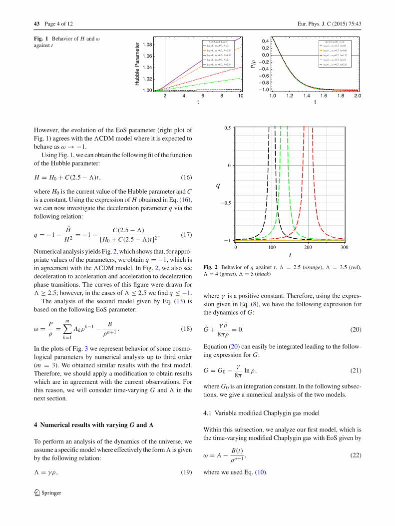
In the first model, given by the EoS (10), we obtain thebehavior of the Hubble parameter and the EoS parameterω = P/ρ by using a numerical analysis which is representedin Fig. 1. The left plot of Fig. 1 shows a typical time evolutionof the Hubble parameter. It is found that the value of Hdecreases with the increasing of the value of �. For � <

2.5, the Hubble parameter is an increasing function of time.� = 2.5 yields the constant H , while for � > 2.5 the Hubbleparameter is a decreasing function of the time.

Since one would expect the Hubble parameter to decreasewith time and become constant at the present epoch, thismodel is not in good agreement with observational data.

123

43 Page 4 of 12 Eur. Phys. J. C (2015) 75 :43

Fig. 1 Behavior of H and ω

against t

However, the evolution of the EoS parameter (right plot ofFig. 1) agrees with the �CDM model where it is expected tobehave as ω → −1.

Using Fig. 1, we can obtain the following fit of the functionof the Hubble parameter:

H = H0 + C(2.5 − �)t, (16)

where H0 is the current value of the Hubble parameter and Cis a constant. Using the expression of H obtained in Eq. (16),we can now investigate the deceleration parameter q via thefollowing relation:

q = −1 − H

H2 = −1 − C(2.5 − �)

[H0 + C(2.5 − �)t]2 . (17)

Numerical analysis yields Fig. 2, which shows that, for appro-priate values of the parameters, we obtain q = −1, which isin agreement with the �CDM model. In Fig. 2, we also seedeceleration to acceleration and acceleration to decelerationphase transitions. The curves of this figure were drawn for� ≥ 2.5; however, in the cases of � ≤ 2.5 we find q ≤ −1.

The analysis of the second model given by Eq. (13) isbased on the following EoS parameter:

ω = P

ρ=

m∑k=1

Akρk−1 − B

ρn+1 . (18)

In the plots of Fig. 3 we represent behavior of some cosmo-logical parameters by numerical analysis up to third order(m = 3). We obtained similar results with the first model.Therefore, we should apply a modification to obtain resultswhich are in agreement with the current observations. Forthis reason, we will consider time-varying G and � in thenext section.

4 Numerical results with varying G and �

To perform an analysis of the dynamics of the universe, weassume a specific model where effectively the form � is givenby the following relation:

� = γρ, (19)

Fig. 2 Behavior of q against t . � = 2.5 (orange), � = 3.5 (red),� = 4 (green), � = 5 (black)

where γ is a positive constant. Therefore, using the expres-sion given in Eq. (8), we have the following expression forthe dynamics of G:

G + γ ρ

8πρ= 0. (20)

Equation (20) can easily be integrated leading to the follow-ing expression for G:

G = G0 − γ

8πln ρ, (21)

where G0 is an integration constant. In the following subsec-tions, we give a numerical analysis of the two models.

4.1 Variable modified Chaplygin gas model

Within this subsection, we analyze our first model, which isthe time-varying modified Chaplygin gas with EoS given by

ω = A − B(t)

ρn+1 , (22)

where we used Eq. (10).

123

Eur. Phys. J. C (2015) 75 :43 Page 5 of 12 43

Fig. 3 Behavior of H , ω and q against t

Fig. 4 Behavior of H against t .Model 1

The plots of Fig. 4 show that the Hubble parameter inthis model is a decreasing function of time The first plotshows that increasing α increases the value of H ; thereforewe find that higher order terms of gravity increase the valueof the Hubble parameter. The second plot deals with the vari-ation of the parameter A. It has been shown that increasing Aincreases the value of H . In the third plot we look at how theHubble parameter changes with n. It is clear that the variationof H depends on the time period. During the period whent < 5, increasing n increases the value of H ; but for t > 5,increasing n decreases the value of H . Finally, in the last plotwe can see the variation of H with ω0 and ω1. In the plotsof Fig. 5 we see the evolution of the deceleration parameterwith various values of α, A, n, ω0, and ω1. In all cases we seethat q takes value between −1 and 0, which is in agreementwith current observational data. So in this case there is noacceleration to deceleration phase transition.

In Fig. 6 we draw the EoS parameter versus time. Wesee from the first plot that increasing α decreases the valueof ω = P/ρ. It is illustrated that higher values of α makeω → −1 faster than lower values of α. A similar situationhappens by varying A (at least for the late time behavior).

The third plot of Fig. 6 shows the variation of ω with n.The first and the second plots were drawn for n = 0.1 andn = 0.3, respectively, causing ω to be a decreasing functionof time and eventually asymptotically approach constant neg-ative values. But, for different values of n and ω, the situationis different, as illustrated in the third and fourth plots of Fig. 6.

Finally, in Fig. 7 we draw the variation of G/G versustime. According to the most observational data, we have [82]∣∣∣∣ G

G

∣∣∣∣ ≤ 1.3 × 10−12 year−1. (23)

The plots of Fig. 7 show good agreement with the observa-tional constraint given in Eq. (23).

Therefore, we can conclude that the first model agreeswith observational data with the exception of the results ofthe deceleration parameter.

4.2 Extended Chaplygin gas model

In the second model we use the EoS parameter given inEq. (18). The plots of Fig. 8 show the behavior of Hubbleparameter as a function of time.

123

43 Page 6 of 12 Eur. Phys. J. C (2015) 75 :43

Fig. 5 Behavior of q against t .Model 1

Fig. 6 Behavior of ω against t .Model 1

Fig. 7 Behavior of G/Gagainst t in unit of10−11 year−1. Model 1

We can see that the Hubble parameter is a decreasing func-tion of time. These plots suggest the following general behav-ior for H :

H = H0 − Ct (1 + t), (24)

where C is a positive constant. Using this fit for the Hubbleparameter we can obtain the following expression for thedeceleration parameter q:

q = −1 + C(1 + 2t)

[H0 − Ct (1 + t)]2 . (25)

123

Eur. Phys. J. C (2015) 75 :43 Page 7 of 12 43

Fig. 8 Behavior of H against t .Model 2

We plotted the behavior of the deceleration parameterobtained in Eq. (25) in Fig. 9. We can see that q is neg-ative during the early universe as well as the late universetherefore the universe is accelerating during these two eras.Between these two epochs q is positive, hence the universe isdecelerating. This behavior is in agreement with the �CDMmodel.

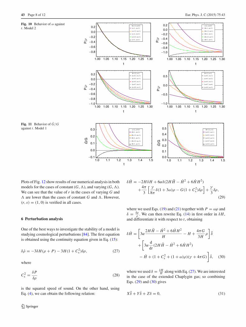
In Fig. 10, we plot the EoS parameter as a function of thetime. The first plot shows that varying of α does not have aneffect on ω in the presence of higher order terms. The sec-ond plot deals with the variation of the constant B. For thecases of B < 3 the EoS parameter is a decreasing functionof time which tends to −1, while for the case of B = 3 theEoS parameter is an increasing function of time which alsogoes to the value of −1. The third plot shows that increas-ing n decreases the value of ω. These plots are obtained form = 3. The last plot contains five curves corresponding tom = 1, . . . , 5 with increasing n. The case of m = 1, whichcorresponds to the modified Chaplygin gas, is illustrated bya violet line. In the plots of Fig. 11 we see the evolution ofG/G is in agreement with observational data.

5 Statefinder diagnostics

In the framework of general relativity, dark energy canexplain the present cosmic acceleration. Except the cosmo-logical constant there are many other candidates of darkenergy (quintom, quintessence, brane, modified gravity etc.).The property of dark energy is that it is model dependent andin order to differentiate different models of dark energy, asensitive diagnostic tool is needed. The Hubble parameter H,and deceleration parameter q are very important quantitieswhich can describe the geometric properties of the universe.Since a > 0, H > 0 means that the universe expands. Also,

Fig. 9 Behavior of q against t . Model 2

ddota > 0, which is q < 0, indicates the accelerated expan-sion of the universe. Since the various dark energy modelsgive H > 0 and q < 0, one needs further evidence to differ-entiate general models of dark energy by investigating cos-mological observational data more accurately. For this aim,we need higher order of time derivatives of the scale factor,a geometrical tool. In Ref. [83] the geometrical statefinderdiagnostic tool was proposed, based on dimensionless param-eters (r, s) which are functions of the scale factor and its timederivative.

These parameters are defined as follows:

r = 1

H3

...a

as = r − 1

3(q − 1

2 4) . (26)

123

43 Page 8 of 12 Eur. Phys. J. C (2015) 75 :43

Fig. 10 Behavior of ω againstt . Model 2

Fig. 11 Behavior of G/Gagainst t . Model 1

Plots of Fig. 12 show results of our numerical analysis in bothmodels for the cases of constant (G, �), and varying (G, �).We can see that the value of r in the cases of varying G and� are lower than the cases of constant G and �. However,(r, s) = (1, 0) is verified in all cases.

6 Perturbation analysis

One of the best ways to investigate the stability of a model isstudying cosmological perturbations [84]. The first equationis obtained using the continuity equation given in Eq. (15):

δρ = −3δH(ρ + P) − 3H(1 + C2s )δρ, (27)

where

C2s = δP

δρ(28)

is the squared speed of sound. On the other hand, usingEq. (4), we can obtain the following relation:

δ H = −2HδH + 6αδ(2H H − H2 + 6H H2)

+4π

3

[ γ

8πδ(1 + 3ω)ρ − G(1 + C2

s )δρ]

+ γ

3δρ,

(29)

where we used Eqs. (19) and (21) together with P = ωρ andδ = δρ

ρ. We can then rewrite Eq. (14) in first order in δH ,

and differentiate it with respect to t , obtaining

δ H =[

3α2H H − H2 + 6H H2

H− H + 4πG

3Hρ

]δ

+[

3αd

dt(2H H − H2 + 6H H2)

− H + (1 + C2s + (1 + ω)ρ)(γ + 4πG)

]δ, (30)

where we used δ = δHH along with Eq. (27). We are interested

in the case of the extended Chaplygin gas; so combiningEqs. (29) and (30) gives

X δ + Y δ + Zδ = 0, (31)

123

Eur. Phys. J. C (2015) 75 :43 Page 9 of 12 43

Fig. 12 r–s. Top panelscorrespond to the cases ofconstant G and � for model 1and model 2, respectively.Bottom panels correspond to thecases of varying G and � formodel 1 and model 2,respectively

0.05 0.04 0.03 0.02 0.01

1.01

1.02

1.03

1.04

1.05

sr

0.16 0.14 0.12 0.10 0.08 0.06 0.04

1.04

1.06

1.08

1.10

1.12

1.14

s

r

0.30 0.35 0.40 0.45 0.50 0.550.50

0.55

0.60

0.65

0.70

0.75

s

r

0.06 0.08 0.10 0.12 0.14 0.16 0.18 0.20

0.84

0.86

0.88

0.90

0.92

0.94

s

r

where

X ≡(

5 − 2H

H2

)

×[

3α2H H − H2 + 6H H2

H− H + 4πG

3Hρ

], (32)

Y ≡(

5 − 2H

H2

) {3α

d

dt(2H H − H2 + 6H H2)

−H + [1 + C2s + (1 + ω)ρ](γ + 4πG)

}, (33)

Z ≡ 12H + 2H

H+ γ

6π(1 + 3ω) − 4πG

3(1+C2

s )+ γ

3− 2.

(34)

Then, using Eqs. (4) and (24), we can obtain a time-dependent equation to investigate the perturbation evolution.We can see from Fig. 13 that perturbations will grow form > 1. However, after long time, they lead to a constant.Moreover, the analysis of the squared speed of sound C2

sshows that the model is stable at all time. In Fig. 14 we haveplotted the behavior of the squared speed of the sound forthree different values of m, in particular m = 1, m = 2, andm = 3.

In the case of m = 1, which corresponds to MCG, wehave constant squared sound speed at initial time increas-

Fig. 13 Typical behavior of δ in terms of t for the extended Chaplygingas. m = 1 (solid), m = 2 (dotted), m = 3 (dashed)

ing at the late time. For the case of m = 2, i.e. a quadraticbarotropic fluid, we see that the value of the squared soundspeed increases dramatically at the early universe and isdecreasing at later stages to a constant value. A similar behav-ior is observed for the case of m = 3. Therefore, we canconclude that the squared sound speed is positive for thesemodels, and hence stable.

123

43 Page 10 of 12 Eur. Phys. J. C (2015) 75 :43

(a) (b) (c)

Fig. 14 Typical behavior of squared sound speed in terms of t for the extended Chaplygin gas. a m = 1, b m = 2, c m = 3

7 Conclusion

In this work, we considered higher order f (R) gravity withtime-dependent G and �. We assumed the Chaplygin gasas a candidate for dark energy and considered two mod-els to describe the evolution of our universe. The first onewas the variable modified Chaplygin gas model (VMCG).The constant B in ordinary MCG is a time-dependentquantity in the context of VMCG. The second model wasthe extended Chaplygin gas. This is indeed an extendedversion of MCG recovering higher order barotropic fluidEoS.

We assumed the specific case where � is proportional tothe energy density and analyzed the Hubble, the deceleration,and the EoS parameters. We found that varying G and � fitthe observational data compared to the cases of constant Gand �.

We also found that the extended Chaplygin gas is amore appropriate model compared to the variable modifiedChaplygin gas model. We can see also an acceleration todeceleration phase transition in the extended Chaplygin gasmodel.

Finally, we investigated the evolution of the density per-turbations by looking at perturbed Friedmann equations. Wealso confirmed the stability of the extended Chaplygin gasby investigating the square of the speed of sound. In sum-mary, we think that the higher order corrected extendedChaplygin gas with time-dependent G and � as a pos-sible model enables one to describe the evolution of ouruniverse.

Open Access This article is distributed under the terms of the CreativeCommons Attribution License which permits any use, distribution, andreproduction in any medium, provided the original author(s) and thesource are credited.Funded by SCOAP3 / License Version CC BY 4.0.

References

1. P. de Bernardis et al., A flat Universe from high-resolution mapsof the cosmic microwave background radiation. Nature 404, 955(2000)

2. S. Perlmutter et al., Measurements of and � from 42 high-redshift supernovae. Astrophys. J. 517, 565 (1999)

3. A.G. Riess et al., Observational evidence from Supernovae for anaccelerating universe and a cosmological constant. Astron. J. 116,1009 (1998)

4. U. Seljak et al., Cosmological parameter analysis including SDSSLy α forest and galaxy bias: constraints on the primordial spectrumof fluctuations, neutrino mass, and dark energy. Phys. Rev. D 71,103515 (2005)

5. P. Astier et al., The Supernova legacy survey: measurement of m ,� and w from the first year data set. Astron. Astrophys. 447, 31(2006)

6. C.L. Bennett et al., First-year Wilkinson microwave anisotropyprobe (WMAP) observations: preliminary maps and basic results.Astrophys. J. Suppl. Ser. 148, 1 (2003)

7. D.N. Spergel et al., First-year Wilkinson microwave anisotropyprobe (WMAP) observations: determination of cosmologicalparameters. Astrophys. J. Suppl. Ser. 148, 175 (2003)

8. E. Komatsu et al., Five-year Wilkinson microwave anisotropy probeobservations: cosmological interpretation. Astrophys. J. Suppl.180, 330 (2009)

9. Planck Collaboration, P.A.R. Ade et al., Planck 2013 results. XVI.Cosmological parameters. Astron. Astrophys. 571, A16 (2014)

10. M. Tegmark et al., Cosmological parameters from SDSS andWMAP. Phys. Rev. D 69, 103501 (2004)

11. K. Abazajian et al., The second data release of the sloan digital skysurvey. Astron. J. 128, 502 (2004)

12. J.K. Adelman-McCarthy et al., The sixth data release of the sloandigital sky survey. Astrophys. J. Suppl. Ser. 175, 297 (2008)

13. S.W. Allen et al., Constraints on dark energy from Chandra obser-vations of the largest relaxed galaxy clusters. Mon. Not. R. Astron.Soc. 353, 457 (2004)

14. E.J. Copeland, M. Sami, S. Tsujikawa, Dynamics of dark energy.Int. J. Mod. Phys. D 15, 1753 (2006)

15. S. Nobbenhuis, Categorizing different approaches to the cosmo-logical constant problem. Found. Phys. 36, 613 (2006)

16. S. del Campo, R. Herrera, D. Pavon, Interacting models may bekey to solve the cosmic coincidence problem. J. Cosmol. Astropart.Phys. 0901, 020 (2009)

123

Eur. Phys. J. C (2015) 75 :43 Page 11 of 12 43

17. M.S. Berger, H. Shojae, Interacting dark energy and the cosmiccoincidence problem. Phys. Rev. D 73, 083528 (2006)

18. K. Griest, Toward a possible solution to the cosmic coincidenceproblem. Phys. Rev. D 66, 123501 (2002)

19. M. Jamil, A. Sheykhi, M.U. Farooq, Thermodynamics of interact-ing entropy-corrected holographic dark energy in a non-flat FRWuniverse. Int. J. Mod. Phys. D 19, 1831 (2010)

20. T. Padmanabhan, Cosmological constant—the weight of the vac-uum. Phys. Rep. 380, 235 (2003)

21. V. Sahni, A.A. Starobinsky, The case for a positive cosmologicallambda-term. Int. J. Mod. Phys. D 9, 373 (2000)

22. B. Ratra, P.J.E. Peebles, Cosmological consequences of a rollinghomogeneous scalar field. Phys. Rev. D 37, 3406 (1988)

23. C. Wetterich, Cosmology and the fate of dilatation symmetry. Nucl.Phys. B 302, 668 (1988)

24. M. Khurshudyan, E. Chubaryan, B. Pourhassan, Interactingquintessence models of dark energy. Int. J. Theor. Phys. 53, 2370(2014)

25. C. Armendariz-Picon, V. Mukhanov, P.J. Steinhardt, A dynamicalsolution to the problem of a small cosmological constant and late-time cosmic acceleration. Phys. Rev. Lett. 85, 4438 (2000)

26. A. Sen, Remarks on tachyon driven cosmology. Phys. Scr. T117,70 (2005)

27. A.Y. Kamenshchik, U. Moschella, V. Pasquier, An alternative toquintessence. Phys. Lett. B 511, 265 (2001)

28. M.C. Bento, O. Bertolami, A.A. Sen, Generalized Chaplygin gas,accelerated expansion and dark energy matter unification. Phys.Rev. D 66, 043507 (2002)

29. L. Xu, J. Lu, Y. Wang, Revisiting generalized Chaplygin gas asa unified dark matter and dark energy model. Eur. Phys. J. C 72,1883 (2012)

30. J.D. Barrow, The deflationary universe: an instability of the de Sitteruniverse. Phys. Lett. B 180, 335 (1986)

31. J.D. Barrow, String-driven inflationary and deflationary cosmolog-ical models. Nucl. Phys. B 310, 743 (1988)

32. N. Ogawa, A note on classical solution of Chaplygin-gas as D-brane. Phys. Rev. D 62, 085023 (2000)

33. H. Saadat, B. Pourhassan, Effect of varying bulk viscosity on gen-eralized Chaplygin gas. Int. J. Theor. Phys. 53, 1168 (2014)

34. X.-H. Zhai, Y.-D. Xu, X.-Z. Li, Viscous generalized Chaplygin gas.Int. J. Mod. Phys. D 15, 1151 (2006)

35. Y.D. Xu et al., Generalized Chaplygin gas model with or with-out viscosity in the ww′ plane. Astrophys. Space Sci. 337, 493(2012)

36. U. Debnath, A. Banerjee, S. Chakraborty, Role of modified Chap-lygin gas in accelerated universe. Class. Quantum Gravity 21, 5609(2004)

37. H. Saadat, B. Pourhassan, FRW bulk viscous cosmology with mod-ified Chaplygin gas in flat space. Astrophys. Space Sci. 343, 783(2013)

38. J. Naji, B. Pourhassan, A.R. Amani, Effect of shear and bulk vis-cosities on interacting modified Chaplygin gas cosmology. Int. J.Mod. Phys. D 23, 1450020 (2013)

39. J. Sadeghi, H. Farahani, Interaction between viscous varying mod-ified cosmic Chaplygin gas and tachyonic fluid. Astrophys. SpaceSci. 347, 209 (2013)

40. B. Pourhassan, Viscous modified cosmic Chaplygin gas cosmol-ogy. Int. J. Mod. Phys. D 22, 1350061 (2013)

41. J. Sadeghi, B. Pourhassan, M. Khurshudyan, H. Farahani, Time-dependent density of modified cosmic Chaplygin gas with cosmo-logical constant in non-flat universe. Int. J. Theor. Phys. 53, 911(2014)

42. H. Saadat, B. Pourhassan, FRW bulk viscous cosmology with mod-ified cosmic Chaplygin gas. Astrophys. Space Sci. 344, 237 (2013)

43. M.R. Setare, Holographic Chaplygin gas model. Phys. Lett. B 648,329 (2007)

44. J. Sadeghi, B. Pourhassan, Z. Abbaspour Moghaddam, Interactingentropy-corrected holographic dark energy and IR cut-off length.Int. J. Theor. Phys. 53, 125 (2014)

45. M.R. Setare, Interacting holographic generalized Chaplygin gasmodel. Phys. Lett. B 654, 1 (2007)

46. E.V. Linder, R.J. Scherrer, Aetherizing lambda: barotropic fluidsas dark energy. Phys. Rev. D 80, 023008 (2009)

47. F. Rahaman, M. Jamil, K. Chakraborty, Revisiting the classicalelectron model in general relativity. Astrophys. Space Sci. 331,191 (2011)

48. B. Pourhassan, E.O. Kahya, Extended Chaplygin gas model.Results Phys. 4, 101 (2014)

49. E.O. Kahya, B. Pourhassan, Observational constraints on theextended Chaplygin gas inflation. Astrophys. Space Sci. 353, 677(2014)

50. S. Nojiri, S.D. Odintsov, Introduction to modified gravity and grav-itational alternative for dark energy. Int. J. Geom. Methods Mod.Phys. 4, 115 (2007)

51. K. Karami, M.S. Khaledian, Reconstructing f (R) modified gravityfrom ordinary and entropy-corrected versions of the holographicand new agegraphic dark energy models. JHEP 3, 86 (2011)

52. M.R. Setare, The holographic dark energy in non-flat Brans–Dickecosmology. Phys. Lett. B 644, 99 (2007)

53. M.R. Setare, M. Jamil, Correspondence between entropy-correctedholographic and Gauss–Bonnet dark energy models. Europhys.Lett. 92, 49003 (2010)

54. A. Pasqua, I. Khomenko, Interacting Ricci logarithmic entropy-corrected holographic dark energy in Brans–Dicke cosmology. Int.J. Theor. Phys. 344, 3981 (2013)

55. C. Deffayet, G. Dvali, G. Gabadadze, Accelerated universe fromgravity leaking to extra dimensions. Phys. Rev. D 65, 044023(2002)

56. V. Sahni, Y. Shtanov, Braneworld models of dark energy. J. Cosmol.Astropart. Phys. 11, 14 (2003)

57. A. Pasqua, S. Chattopadhyay, A study on modified holographicRicci dark energy in modified f (R) Horava–Lifshitz gravity. Can.J. Phys. 91, 351 (2013)

58. B. Li, T.P. Sotiriou, J.D. Barrow, Large-scale structure in f (T )

gravity. Phys. Rev. D 83, 104017 (2011)59. K. Bamba, C.Q. Geng, C.C. Lee, L.W. Luo, Equation of state for

dark energy in f (T ) gravity. J. Cosmol. Astropart. Phys. 1101, 021(2011)

60. T.P. Sotiriou, V. Faraoni, f (R) theories of gravity. Rev. Mod. Phys.82, 451 (2010)

61. A. Jawad, S. Chattopadhyay, A. Pasqua, A holographic reconstruc-tion of the modified f (R) Horava–Lifshitz gravity with scale factorin power-law form. Astrophys. Space Sci. 346, 273 (2013)

62. S. Capozziello, S. Carloni, A. Troisi, Quintessence without scalarfields. Recent Res. Dev. Astron. Astrophys. 1, 625 (2003)

63. N. Arkani-Hamed, H.C. Cheng, M.A. Luty, S. Mukohyama, Ghostcondensation and a consistent IR modification of gravity. JHEP 05,043528 (2004)

64. A. Jawad, S. Chattopadhyay, A. Pasqua, Reconstruction of f (G)

gravity with the new agegraphic dark-energy model. Eur. Phys. J.Plus 128, 88 (2012)

65. R. Myrzakulov, FRW cosmology in f (R, T ) gravity. Eur. Phys. J.C 72, 2203 (2012)

66. S. Chattopadhyay, A. Pasqua, Holographic DBI-essence darkenergy via power-law solution of the scale factor. Int. J. Theor.Phys. 52, 3945 (2013)

67. A. Pasqua, S. Chattopadhyay, Logarithmic entropy-corrected holo-graphic dark energy in Horava–Lifshitz cosmology with Granda–Oliveros cut-off. Astrophys. Space Sci. 348, 541 (2013)

68. A. Pasqua, S. Chattopadhyay, New agegraphic dark energy modelin chameleon Brans–Dicke cosmology for different forms of thescale factor. Astrophys. Space Sci. 348, 283 (2013)

123

43 Page 12 of 12 Eur. Phys. J. C (2015) 75 :43

69. M. Khurshudyan, A. Pasqua, B. Pourhassan, Higher derivative cor-rections of f (R) gravity with varying equation of state in the caseof variable G and �. Can. J. Phys. arXiv:1401.6630

70. M. Jamil, U. Debnath, FRW cosmology with variable G andlambda. Int. J. Theor. Phys. 50, 1602 (2011)

71. M. Jamil, F. Rahaman, M. Kalam, Cosmic coincidence problemand variable constants of physics. Eur. Phys. J. C 60, 149 (2009)

72. B.C. Paul, P.S. Debnath, Viscous cosmologies with variable G and� in R2 gravity. arXiv:1105.3307

73. J. Lu, L. Xu, Y. Wu, M. Liu, Reduced modified Chaplygin gascosmology. arXiv:1312.0779

74. J. Lu, L. Xu, J. Li, B. Chang, Y. Gui, H. Liu, Constraints on modifiedChaplygin gas from recent observations and a comparison of itsstatus with other models. Phys. Lett. B 662, 87 (2008)

75. A.M. Velasquez-Toribio, M.L. Bedran, Fitting cosmological datato the function q(z) from GR theory: modified Chaplygin gas. Braz.J. Phys. 41, 59 (2011)

76. J. Lu, L. Xu, Y. Wu, M. Liu, Combined constraints on modifiedChaplygin gas model from cosmological observed data: MarkovChain Monte Carlo approach. Gen. Relativ. Gravit. 43, 819 (2011)

77. L. Xu, Y. Wang, H. Noh, Modified Chaplygin gas as a unified darkmatter and dark energy model and cosmic constraints. Eur. Phys.J. C 72, 1931 (2012)

78. S. Chakraborty, U. Debnath, C. Ranjit, Observational constraintsof modified Chaplygin gas in loop quantum cosmology. Eur. Phys.J. C 72, 2101 (2012)

79. D. Panigrahi, B.C. Paul, S. Chatterjee, Constraining modifiedChaplygin gas parameters. arXiv:1305.7204

80. B.C. Paul, P. Thakur, Observational constraints on modified Chap-lygin gas from cosmic growth. J. Cosmol. Astropart. Phys. 1311,052 (2013)

81. A.A. Usmani, P.P. Ghosh, U. Mukhopadhyay, P.C. Ray, S. Ray, Thedark energy equation of state. Mon. Not. R. Astron. Soc. Lett. 386,L92–95 (2008)

82. H. Wei, H.-Y. Qi, X.-P. Ma, Constraining f (T ) theories with thevarying gravitational constant. Eur. Phys. J. C 72, 2127 (2012)

83. V. Sahni, T.D. Saini, A.A. Starobinsky, U. Alam, Statefinder—anew geometrical diagnostic of dark energy. JETP Lett. 77, 201(2003)

84. A. Vale, J.P.S. Lemos, Linear perturbations in a universe with acosmological constant. Mon. Not. R. Astron. Soc. 325, 1197 (2001)

123