Linearis felt´ eteles, szepar´ abilis konk´ av...

•First •Prev •Next •Last •Go Back •Full Screen •Close •Quit

Linearis felteteles, szeparabilis konkavminimalizalasi feladat

alkalmazasai es megoldasa

Illes [email protected]

Differencialegyenletek TanszekBudapesti Muszaki es Gazdasagtudomanyi Egyetem

Budapest2010. november 23.

mailto:[email protected]


Outline

• Linearly constrained, separable concave minimization problem (definition,known results, solution methods, practical problems)

• Elementary properties of concave functions

• Linear relaxation of concave functions

• Linear programming relaxation of the original problem

• Optimality criteria of the relaxed linear programming problem

• Linear approximation of concave functions (example)

• Necessary optimality condition

• Sufficient optimality condition

• Test points

• Procedure for checking the optimality of a basic feasible solution

Illes Tibor BME DE


Linearly constrained, separable concave minimization problem

min F (x)Ax ≤ b

l ≤ x ≤ u

(P )

where A ∈ IRm×n, b ∈ IRm, l,u ∈ IRn and l ≥ 0.

Objective function: F (x) :=n∑

j=1fj(xj), where fj : IR → IR are concave

functions and for the domain of fj [lj, uj] ⊆ Dfj holds. Let us introduce the

sets A := {x ∈ IRn : Ax ≤ b} and T := {x ∈ IRn : l ≤ x ≤ u}.

Feasible solution set: P = A ∩ Tset of the optimal solutions: P∗ := {x ∈ P : F (x) ≤ F (x), x ∈ P}

Known results:

1. If P 6= ∅ then P∗ 6= ∅ holds, since F is continuous and P is bounded andclosed.2. There is optimal solution at a vertex of the polytop P . (Luenberger, 1973)

3. The problem (P ) is in the class of NP-complete problems. (Murty and Kabadi, 1987)

Illes Tibor BME DE


Practical problems

Several practical problem can be formulated by problem (P ) like

• some control problems (e.g. Apkarian and Tuan, 1999),

• concave knapsack problems (e.g. More and Vavasis, 1990/91),

• some production and transportation problems (e.g. Kuno and Utsunomiya,2000),

• production planning problems (e.g. Liu, Sahinidis and Shectman, 1996),

• process network synthesis problems (e.g. Friedler, Fan and Imreh, 1998),

• some network flow problems (e.g. Yajima and Konno, 1999),

• ...

Illes Tibor BME DE


Solution methods

• listing vertices of the polyhedronP (e.g. Dyer, 1983; Dyer and Proll, 1977),

• cutting plane methods (e.g. Hoffman, 1981; Tuy, Thieu and Thai, 1985),

• branch-and-bound algorithms, BB (e.g. Falk and Soland, 1969; Shectmanand Sahinidis, 1998; Phillips and Rosen, 1993; Locatelli and Thoai, 2000)and

• other methods ...

Illes Tibor BME DE


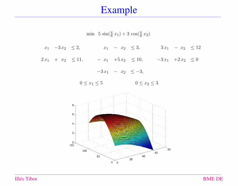
Example

min 5 sin(π6 x1) + 3 cos(π6 x2)

x1 −3x2 ≤ 2, x1 − x2 ≤ 3, 3x1 − x2 ≤ 12

2x1 + x2 ≤ 11, − x1 +5x2 ≤ 10, −3x1 +2x2 ≤ 0

−3x1 − x2 ≤ −3,

0 ≤ x1 ≤ 5 0 ≤ x2 ≤ 3

Illes Tibor BME DE


Elementary properties of concave functionsTheorem. Let f be one dimensional function on interval I ⊂ Df .The following statements are equivalent

(a) Function f is concave on interval I.

(b) Let x, y ∈ I, x 6= y and m(x, y) = f(y)−f(x)y−x . If a, b, c ∈ I,

a < b < c then the following holds m(a, b) ≥ m(a, c) ≥ m(b, c).

(c) For any t ∈ I , mt(x) = m(t, x) function is decreasing on I \ {t}.(a) If a, b, c ∈ I, a < b < c then m(a, b) ≥ m(b, c). •

Theorem. Let f be one dimensional concave function on open intervalI ⊂ Df , then

(a) Function f is continuous on interval I .

(b) At any t ∈ I the function is left and right differentiable andf ′−(t) ≥ f ′+(t).

(c) If a, b,∈ I, a < b then f ′+(a) ≥ m(a, b) ≥ f ′−(b), moreover, if fis strict concave on interval I, then f ′+(a) > m(a, b) > f ′−(b). •

Illes Tibor BME DE


Linear relaxation of concave functionsBB-type linear relaxation of the concave functions fj : IR→ IR on the closed interval [lj , uj ] is

gj(xj) = m(lj , uj) (xj− lj)+fj(lj) =fj(uj)− fj(lj)

uj − ljxj +

(fj(lj)−

fj(uj)− fj(lj)uj − lj

lj

)= cj xj +dj ,

where cj = m(lj , uj) and dj = fj(lj) −m(lj , uj) lj . Then the objective function F (x) =n∑j=1

fj(xj)

is approximated by the linear function

G(x) =

n∑j=1

gj(xj) =

n∑j=1

(cj xj + fj(lj)− cj lj) = cTx + (F (l)− cT l) = cTx + δ

on the set P = A ∩ T , where δ = F (l)− cT l. It is easy to show that

F (x) ≥ G(x) = cTx + δ, holds for all x ∈ P .

Example (continue) x1 ∈ [0, 5] and x2 ∈ [0, 3]

f1(x1) = 5 sin(π

6x1) : c1 =

5 sin(π6 5)

5=

1

2, d1 = 0 ⇒ g1(x1) =

1

2x1

f2(x2) = 3 cos(π

6x2) : c2 =

3 cos(π6 3)− 3 cos(0)

3= −1, d2 = 3 ⇒ g2(x2) = −x2 + 3

Illes Tibor BME DE


Linear relaxation of the problemLower bound for the objective value of (P ) can be computed using the following linear program-ming problem

minx∈P

cTx + δ (PLP )

Proposition. Let x ∈ P∗LP and assume that F ∈ C(int(T )) then

β = cT x + δ = G(x) ≤ F (x) ≤ F (x) + (∇F (x))T (x− x)

holds for all x ∈ P . •

Example (continue)

min 12 x1 − x2 + 3

x1 −3x2 ≤ 2, x1 − x2 ≤ 3, 3x1 − x2 ≤ 12

2x1 + x2 ≤ 11, − x1 +5x2 ≤ 10, −3x1 +2x2 ≤ 0

−3x1 − x2 ≤ −3,

0 ≤ x1 ≤ 5 0 ≤ x2 ≤ 3

Optimal solution: x1 = 1.53846, x2 = 2.30769, and G(x) = 1.46154

G(x) = 1.46154 ≤ F (x) = 5 sin(π6 x1) + 3 cos(π6 x2) ≤ 1.8135x1 − 1.4687x2 + 5.269

Illes Tibor BME DE


Linear programming relaxation of the original problem

Let us consider the relaxed LP problem (and it’s dual) of (P ) in the following form

min cTxAx ≤ b

l ≤ x ≤ u

(PLP )max −bTy + lTz− uT s−ATy + z− s = c

y ≥ 0, z ≥ 0, s ≥ 0

(DLP )

Set of the dual feasible solutions: D = {(y, z, s) : −ATy + z− s = c, y ≥ 0, z ≥ 0, s ≥ 0}

Weak Duality Theorem. Let x ∈ P and (y, z, s) ∈ D vectors then

cTx ≥ −bTy + lTz− uT s

inequality holds. Previous inequality holds with equality if and only if

0 = cTx + bTy − lTz + uT s = yT (b− Ax) + zT (x− l) + sT (u− x). •

Optimality criteria: Ax ≤ b, l ≤ x ≤ u−ATy + z− s = c, y ≥ 0, z ≥ 0, s ≥ 0

y (b− Ax) = 0, z (x− l) = 0, s (u− x) = 0,

P∗c = {x∗ ∈ P : cTx∗ ≤ cTx, x ∈ P} is the set of the optimal solutions of the problem (PLP ).

Index sets: J = JB ∪ JN = JB ∪ (J lN ∪ JuN ), JB ∩ JN = ∅.

Basic vectors {aj : j ∈ JB} are linearly independent. Let x ∈ P basic feasible solution, then

xB = B−1 b−∑j∈J l

N

lj aj −∑j∈J u

N

uj aj , where aj = B−1aj .

Illes Tibor BME DE


Optimality criteria of the relaxed linear programming problem

Let x∗ ∈ P∗c be a basic solution belonging to the basis B and y∗ = cTBB−1 ≥ 0, we get that

• in case of j ∈ JB, lj < x∗j < uj , zj = 0 and sj = 0 hold and thus −aTj y = cj ,

• in case of j ∈ J lN , lj = x∗j , zj ≥ 0 and sj = 0 hold and thus zj = cj + aTj y ≥ 0,

• in case of j ∈ J uN , uj = x∗j , zj = 0 and sj ≥ 0 hold and thus −sj = cj + aTj y ≤ 0.

Finally, we obtain a basic solution x∗ ∈ P , which is optimal if and only if

y∗ = cTBB−1 ≥ 0 (1)

− cTBB−1aj ≤ cj , any j ∈ J lN and (2)

− cTBB−1aj ≥ cj , any j ∈ J uN (3)

hold.

Let us consider the set of all objective function coefficients of linear programs for which thecurrent basic solution, x∗ ∈ P is an optimal basic solution

CB = {c ∈ IRn : constraints (1)− (3) are satisfied} 6= ∅

Example (continue) Sensitivity analysis shows that if c1 ∈ [0.2, 1.5] and c2 ∈ [−2.5,−0.33] thenx1 = 1.53846, x2 = 2.30769 remains optimal solution of the relaxed LP (c) problem.

Illes Tibor BME DE


Linear approximation of concave functions

General linear approximation of the concave functions fj : IR → IR on the closed interval [aj , bj ]is

hj(xj) = m(aj , bj) (xj − aj) + fj(aj) = hj xj + rj

where lj ≤ aj < bj ≤ uj , hj = m(aj , bj) and rj = fj(aj)−m(aj , bj) aj . Then for the function

H(x) =

n∑j=1

hj(xj) =

n∑j=1

(hj xj + fj(aj)− hj aj) = hTx + (F (a)− hTa) = hTx + %,

where % = F (a)− hTa, and the following inequalities holds

F (x) ≥ H(x), for all x ∈ P(a,b), and F (x) ≤ H(x), for all x ∈ P \ P(a,b),

where a,b ∈ T , a < b and P(a,b) = A ∩ {x ∈ IRn : a ≤ x ≤ b}.

Set of the normal vectors of the general linear approximations:

Hf := {h ∈ IRn : hj = f ′j,+(t), t ∈ [lj , uj)} ∪ {h ∈ IRn : hj = f ′j,−(t), t ∈ (lj , uj ]} ∪{h ∈ IRn : hj = m(aj , bj), lj ≤ aj < bj ≤ uj}

Question. Is there any relations between the sets CB and Hf ?

Illes Tibor BME DE


Linear approximation of concave function

l j

k

fj

k

fj

p uj

k xj

II.I.

Illes Tibor BME DE


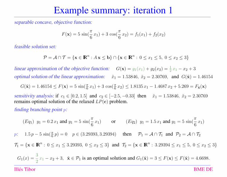
Example summary: iteration 1separable concave, objective function:

F (x) = 5 sin(π

6x1) + 3 cos(

π

6x2) = f1(x1) + f2(x2)

feasible solution set:

P = A ∩ T = {x ∈ IRn : Ax ≤ b} ∩ {x ∈ IRn : 0 ≤ x1 ≤ 5, 0 ≤ x2 ≤ 3}

linear approximation of the objective function: G(x) = g1(x1) + g2(x2) = 12 x1 − x2 + 3

optimal solution of the linear approximation: x1 = 1.53846, x2 = 2.30769, and G(x) = 1.46154

G(x) = 1.46154 ≤ F (x) = 5 sin(π6 x1) + 3 cos(π6 x2) ≤ 1.8135x1 − 1.4687x2 + 5.269 = Fx(x)

sensitivity analysis: if c1 ∈ [0.2, 1.5] and c2 ∈ [−2.5,−0.33] then x1 = 1.53846, x2 = 2.30769remains optimal solution of the relaxed LP (c) problem.

finding branching point p:

(Eq1) y1 = 0.2x1 and y1 = 5 sin(π

6x1) or (Eq2) y1 = 1.5x1 and y1 = 5 sin(

π

6x1)

p: 1.5 p− 5 sin(π6 p) = 0 p ∈ (3.29393, 3.29394) then P1 = A ∩ T1 and P2 = A ∩ T2

T1 = {x ∈ IRn : 0 ≤ x1 ≤ 3.29393, 0 ≤ x2 ≤ 3} and T2 = {x ∈ IRn : 3.29394 ≤ x1 ≤ 5, 0 ≤ x2 ≤ 3}

G1(x) =3

2x1 − x2 + 3, x ∈ P1 is an optimal solution and G1(x) = 3 ≤ F (x) ≤ F (x) = 4.6698.

Illes Tibor BME DE


Example: iteration 2

(LP ) : minx∈P

G(x) optimal solution x1 = 1.53846, x2 = 2.30769, and G(x) = 1.46154

branching point p ∈ (3.29393, 3.29394): (LP1) and (LP2)

(LP1) : minx∈P1

G1(x) x = (1.53846, 2.30769) ∈ P1, G1(x) = 3 < F (x) = 4.6698;

sensitivity analysis: c1 ∈ [1.5,+∞) and c2 ∈ [−1, 0.5]

(LP2) : minx∈P2

G2(x)

G2(x) = g21(x1) + g2

2(x2) = −1.4307x1 + 9.6535− x2 + 3 = −1.4307x1 − x2 + 12.6535

optimal solution x1 = 4.09091, x2 = 2.818182, and G2(x) = 3.982454

G2(x) = 3.982454 < F (x) = 4.4914 and G2(x) ≤ F (x) ≤ −1.4154x1 − 1.5637x2 + 14.6885

Problem T x G(x) F (x) Status(LP ) 0 ≤ x1 ≤ 5, 0 ≤ x2 ≤ 3 (1.53846, 2.30769) 1.46154 4.6698 1(LP1) 0 ≤ x1 ≤ 3.29393, 0 ≤ x2 ≤ 3 (1.53846, 2.30769) 3 4.6698 1(LP2) 3.29394 ≤ x1 ≤ 5, 0 ≤ x2 ≤ 3 (4.09091, 2.818182) 3.982454 4.4914 1

Illes Tibor BME DE


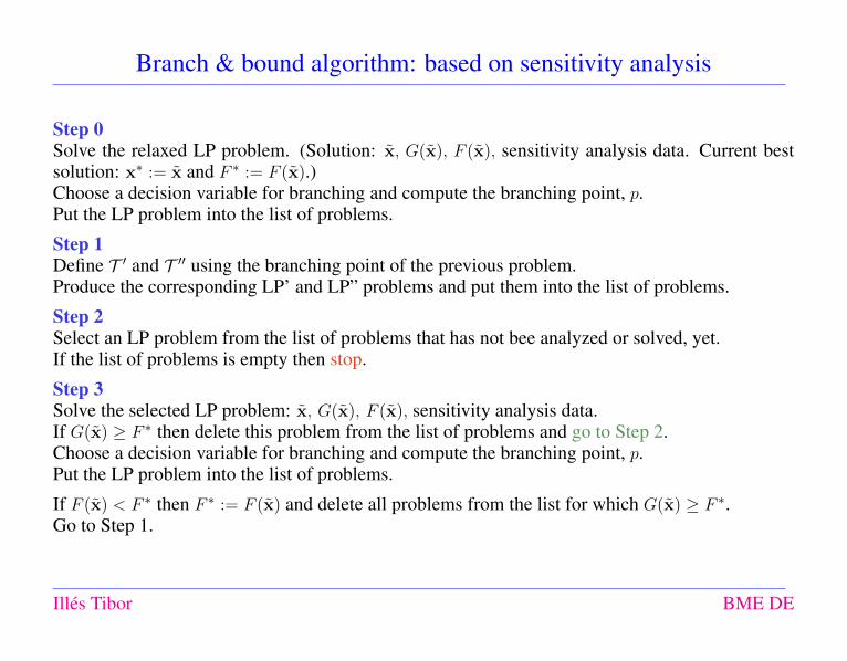
Branch & bound algorithm: based on sensitivity analysis

Step 0Solve the relaxed LP problem. (Solution: x, G(x), F (x), sensitivity analysis data. Current bestsolution: x∗ := x and F ∗ := F (x).)Choose a decision variable for branching and compute the branching point, p.Put the LP problem into the list of problems.

Step 1Define T ′ and T ′′ using the branching point of the previous problem.Produce the corresponding LP’ and LP” problems and put them into the list of problems.

Step 2Select an LP problem from the list of problems that has not bee analyzed or solved, yet.If the list of problems is empty then stop.

Step 3Solve the selected LP problem: x, G(x), F (x), sensitivity analysis data.If G(x) ≥ F ∗ then delete this problem from the list of problems and go to Step 2.Choose a decision variable for branching and compute the branching point, p.Put the LP problem into the list of problems.

If F (x) < F ∗ then F ∗ := F (x) and delete all problems from the list for which G(x) ≥ F ∗.Go to Step 1.

Illes Tibor BME DE


Example: result

Vertex Function value Vertex Function valueP12 = (7

2 ,12) 7.7274 P56 = (20

13 ,3013) 4.6698

P23 = (92 ,

32) 5.6569 P67 = (2

3 , 1) 4.3082

P34 = (235 ,

95) 5.109 P70 = (1, 0) 5.5

P45 = (4511 ,

3111) 4.4914 P01 = (2, 0) 7.3301

Illes Tibor BME DE


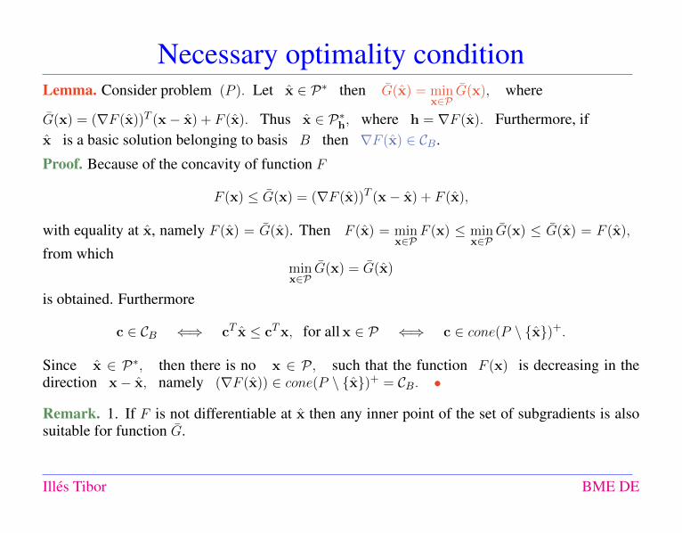
Necessary optimality conditionLemma. Consider problem (P ). Let x ∈ P∗ then G(x) = min

x∈PG(x), where

G(x) = (∇F (x))T (x− x) + F (x). Thus x ∈ P∗h, where h = ∇F (x). Furthermore, ifx is a basic solution belonging to basis B then ∇F (x) ∈ CB.

Proof. Because of the concavity of function F

F (x) ≤ G(x) = (∇F (x))T (x− x) + F (x),

with equality at x, namely F (x) = G(x). Then F (x) = minx∈P

F (x) ≤ minx∈P

G(x) ≤ G(x) = F (x),

from whichminx∈P

G(x) = G(x)

is obtained. Furthermore

c ∈ CB ⇐⇒ cT x ≤ cTx, for allx ∈ P ⇐⇒ c ∈ cone(P \ {x})+.

Since x ∈ P∗, then there is no x ∈ P , such that the function F (x) is decreasing in thedirection x− x, namely (∇F (x)) ∈ cone(P \ {x})+ = CB. •

Remark. 1. If F is not differentiable at x then any inner point of the set of subgradients is alsosuitable for function G.

Illes Tibor BME DE


A property of linear relaxation

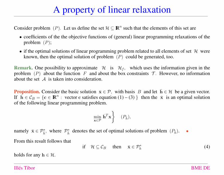
Consider problem (P ). Let us define the set H ⊆ IRn such that the elements of this set are

• coefficients of the the objective functions of (general) linear programming relaxations of theproblem (P );

• if the optimal solutions of linear programming problem related to all elements of set H wereknown, then the optimal solution of problem (P ) could be generated, too.

Remark. One possibility to approximate H is Hf , which uses the information given in theproblem (P ) about the function F and about the box constraints T . However, no informationabout the set A is taken into consideration.

Proposition. Consider the basic solution x ∈ P , with basis B and let h ∈ H be a given vector.If h ∈ CB = {c ∈ IRn : vector c satisfies equation (1) – (3) } then the x is an optimal solutionof the following linear programming problem.

minx∈P

hTx

}(Ph),

namely x ∈ P∗h, where P∗

hdenotes the set of optimal solutions of problem (Ph). •

From this result follows thatif H ⊆ CB then x ∈ P∗h (4)

holds for any h ∈ H.

Illes Tibor BME DE


Sufficient optimality condition

Theorem. Consider the linearly constrained, separable concave minimization problem (P ), andsuppose the functions fj are strictly concave. Let x ∈ P be a basic solution with basis B thatH ⊆ CB holds, then P∗ = {x}.

Proof. Since H ⊆ CB thus x ∈ P∗h holds for any h ∈ H.

There exist global minimal solution x of (P ) which is an extremal point of the set P . Supposethat x 6= x.

Let h = ∇ f(x). Since previous lemma asserts x ∈ P∗h, otherwise x ∈ P∗

h. The following

relations hold,F (x) = G(x) = G(x) > F (x), (5)

which is a contradiction, thus x = x, then P∗ = {x}. •

Remark. The strict inequality comes from the strict concavity. If the condition of strict concavityis removed from the previous Theorem then the inequality (5) will be modified as

F (x) ≥ F (x) = G(x) = G(x) ≥ F (x)

so F (x) = F (x), thus x ∈ P∗, but the equality |P∗| = 1 cannot be guaranteed.

It has been proved that the sufficient optimality condition for a basic solution x ∈ P of problem(P ) with basis B is

H ⊆ CB.

Illes Tibor BME DE


Approximating setHIf the set approximating H is only based on the properties of problem (P ), we can get

Hf = {h ∈ IRn : hj ∈ [f ′j−(uj), f′j+(lj)]}

and H ⊆ Hf holds. Based on the previous result for a basic solution x ∈ P of problem (P ) withbasis B, if H ⊆ Hf ⊆ CB then P∗ = {x}.

Let us determine set approximating H for a given basic solution x ∈ P then

Hf,x = {h ∈ IRn : hj ∈ [clj , cuj ]} (Phillips and Rosen, 1993)

this set (hyper rectangle) will contain the coefficients of all possible relaxed linear functions, where

cuj =

{m(lj , xj), xj 6= ljf ′j+(lj), otherwise and clj =

{m(xj , uj), xj 6= ujf ′j−(uj), otherwise

From the concavity of the function F, we can get the inequalities

f ′j−(uj) ≤ clj = m(xj , uj) ≤ m(lj , xj) = cuj ≤ f ′j+(lj) (6)

and therefore Hf,x ⊆ Hf holds.

2n relaxed LP problems have a common optimal solution ⇐⇒ Hf,x ⊆ CB

extremal points of Hf,x are elements of CB ⇐⇒ Hf,x ⊆ CB

Illes Tibor BME DE


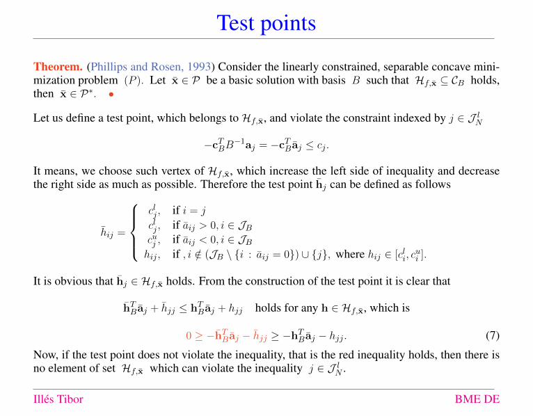
Test points

Theorem. (Phillips and Rosen, 1993) Consider the linearly constrained, separable concave mini-mization problem (P ). Let x ∈ P be a basic solution with basis B such that Hf,x ⊆ CB holds,then x ∈ P∗. •

Let us define a test point, which belongs to Hf,x, and violate the constraint indexed by j ∈ J lN

−cTBB−1aj = −cTBaj ≤ cj .

It means, we choose such vertex of Hf,x, which increase the left side of inequality and decreasethe right side as much as possible. Therefore the test point hj can be defined as follows

hij =

clj , if i = j

clj , if aij > 0, i ∈ JBcuj , if aij < 0, i ∈ JBhij , if , i /∈ (JB \ {i : aij = 0}) ∪ {j}, where hij ∈ [cli, c

ui ].

It is obvious that hj ∈ Hf,x holds. From the construction of the test point it is clear that

hTBaj + hjj ≤ hTBaj + hjj holds for any h ∈ Hf,x, which is

0 ≥ −hTBaj − hjj ≥ −hTBaj − hjj . (7)

Now, if the test point does not violate the inequality, that is the red inequality holds, then there isno element of set Hf,x which can violate the inequality j ∈ J lN .

Illes Tibor BME DE


Test points (continue)

In general, the test point hk for any index k ∈ J lN ∪ JuN will be defined, using sets J +

i , J −i , andi ∈ JB, as follows

hik =

cli, if k ∈ J −i , i ∈ JBcui , if k ∈ J +

i , i ∈ JBclk, if i = k, and k ∈ J lNcuk , if i = k, and k ∈ J uNhi, i /∈ (JB \ {i : aik = 0}) ∪ {k}, where hi ∈ [cli, c

ui ]

where

J +i = {k ∈ J lN : aik < 0} ∪ {k ∈ J uN : aik > 0}, andJ −i = {k ∈ J lN : aik > 0} ∪ {k ∈ J uN : aik < 0}.

Based on these observations, we can get the following proposition.

Proposition. If test point hk does not violate the inequality k ∈ J lN ∪ JuN then no point h ∈ Hf,x

violates either. •

Moreover, in case of j ∈ J lN (j ∈ J uN )

−hTB,j aj > clj (−hTB,j aj < cuj )

the test point hj violates the optimality criteria which belongs to the variable j.

Illes Tibor BME DE


Procedure for checking the optimality of a basic solution

We can determine a test point for testing inequality system hTBB−1 ≥ 0.

Let matrix B = B−1 and let bi denote the ith column of matrix B, then

hji =

cli, if bji > 0, j ∈ JBcui , if bji < 0, j ∈ JBhi, if j ∈ J lN ∪ J

uN ∪ {j ∈ JB : bji = 0} where, hi ∈ [clj , c

uj ]

In this case, if hTj,B bi ≥ 0 holds, then for any vector h ∈ Hf,x the ith nonnegativity condition issatisfied.

Remark. Instead of testing 2n vertices of hyper rectangle Hf,x, it is enough to determine ntest points in order to check whether the inclusion Hf,x ⊆ CB holds or not.

Let us introduce the index set K = {i : hi test point violates ith inequality }.

It is obvious that, the equality K = ∅ leads to Hf,x ⊆ CB, thus x ∈ P∗ holds. The decision,whether basic solution x ∈ P is optimal for the problem (P ), can be performed as follows

1. generate set Hf,x,

2. using matrices B−1 and B−1AN generate test point hj ,

3. check the test points, if there is no index j for which test point hj violates jth conditionthen x is optimal solution for problem (P ).

Question: if any test point hj can be founded which violates jth condition, can we concludethat x ∈ P is not an optimal solution of the problem (P ) ?

Illes Tibor BME DE


Illustration: set CB for different bases

Illes Tibor BME DE


Illustration: a test point violating a constraint

Illes Tibor BME DE


Illustration: projections of the CB sets

Illes Tibor BME DE


Illustration: projections of the CB and the correspondingHf,x sets

Illes Tibor BME DE


Reference

Illes, T., Nagy, A. B., Sufficient optimality criterion for linearly constrained,separable concave minimization problems. J. Optim. Theory Appl. (2005),125:3, 559575.

Illes Tibor BME DE

Linearis felt´ eteles, szepar´ abilis konk´ av...

Documents

Transcript of Linearis felt´ eteles, szepar´ abilis konk´ av...