linear transformation.pdf

Chapter 3

Linear Transformations

In your previous mathematics courses you undoubtedly studied real-valued func-tions of one or more variables. For example, when you discussed parabolas thefunction f(x) = x2 appeared, or when you talked abut straight lines the func-tion f(x) = 2x arose. In this chapter we study functions of several variables,that is, functions of vectors. Moreover, their values will be vectors rather thanscalars. The particular transformations that we study also satisfy a “linearity”condition that will be made precise later.

3.1 Definition and Examples

Before defining a linear transformation we look at two examples. The first isnot a linear transformation and the second one is.

Example 1. Let V = R2 and let W = R. Define f : V → W by f(x1, x2) =x1x2. Thus, f is a function defined on a vector space of dimension 2, withvalues in a one-dimensional space. The notation is highly suggestive; that is,f : V → W indicates that f does something to a vector in V to get a vectorin W . For example, f(1,−1) = −1, f(1, 2) = 2, etc. We will see later thatthis function does not satisfy the “linearity” condition and hence is not a lineartransformation. �

Example 2. Let V = R2 and W = R

3. Define L : V → W by L(x1, x2) =(x1, x2 − x1, x2). Here the function L takes a vector in R2 and transforms itinto a vector in R3. For example, L(1,−1) = (1,−2,−1) and L(2, 6) = (2, 4, 6).This particular function satisfies the linearity condition below, and so would becalled a linear transformation from R2 to R3. �

Definition 3.1. Let V andW be two vector spaces. Let L be a function definedon V with values in W . L will be called a linear transformation if it satisfiesthe following two conditions:

1. L(xxx+ yyy) = L(xxx) + L(yyy), for any two vectors xxx and yyy in V .

109

110 CHAPTER 3. LINEAR TRANSFORMATIONS

2. L(cxxx) = cL(xxx), for any scalar c and vector xxx in V .

Let’s go back to Example 2 and verify that we did indeed have a linear trans-formation. For any xxx = (x1, x2) and yyy = (y1, y2), we have

L(xxx+ yyy) = L[(x1 + y1, x2 + y2)] = [x1 + y1, (x2 + y2)− (x1 + y1), x2 + y2]

= (x1, x2 − x1, x2) + (y1, y2 − y1, y2) = L(xxx) + L(yyy).

Thus, condition 1 holds. Moreover

L(cxxx) = L[(cx1, cx2)] = (cx1, cx2 − cx1, cx2) = c(x1, x2 − x1, x2) = cL(xxx)

Since 1 and 2 hold, L is a linear transformation from R2 to R3. The readershould now check that the function in Example 1 does not satisfy either of thesetwo conditions.

Example 3. Define L : R3 → R2 by L(x1, x2, x3) = (x3 − x1, x1 + x2).

a. Compute L(eee1), L(eee2), and L(eee3).

b. Show L is a linear transformation.

c. Show L(x1, x2, x3) = x1L(eee1) + x2L(eee2) + x3L(eee3).

a. L[(1, 0, 0)] = (−1, 1), L[(0, 1, 0)] = (0, 1), L[(0, 0, 1)] = (1, 0).

b. L(xxx+ yyy) = L[(x1 + y1, x2 + y2, x3 + y3)]

= ((x3 + y3)− (x1 + y1), (x1 + y1) + (x2 + y2))

= (x3 − x1, x1 + x2) + (y3 − y1, y1 + y2)

= L(xxx) + L(yyy)

L(cxxx) = L[(cx1, cx2, cx3)] = (cx3 − cx1, cx1 + cx2)

= c(x3 − x1, x1 + x2) = cL(xxx)

Thus L satisfies conditions 1 and 2 of Definition 3.1, and it is a linear transfor-mation.

c. L(x1, x2, x3) = L(x1eee1 + x2eee2 + x3eee3)

= L(x1eee1) + L(x2eee2) + L(x3eee3)

= x1L(eee1) + x2L(eee2) + x3L(eee3)

Notice that c implies that once L(eeek), k = 1, 2, 3, are known, the fact that L isa linear transformation completely determines L(xxx) for any vector xxx in R3. �

We collect a few facts about linear transformations in the next theorem.

Theorem 3.1. Let L be a linear transformation from a vector space V into avector space W . Then

1. L(000) = 000

3.1. DEFINITION AND EXAMPLES 111

2. L(−xxx) = −L(xxx)

3. L

(

n∑

k=1

akxxxk

)

=n∑

k=1

akL(xxxk)

Proof.

1. Let xxx be any vector in V . Then L(xxx) = L(xxx+000) = L(xxx) + L(000). Adding−L(xxx) to both sides, we have L(000) = 000, where the zero vector on theleft-hand side is in V while the zero vector on the right-hand side is in W .

2. 000 = L(000) = L(xxx− xxx) = L(xxx) + L(−xxx). Thus L(−xxx) = −L(xxx).

3. We show that this formula is true for n = 3 and leave the details of aninduction argument to the reader.

L(a1xxx1 + a2xxx2 + a3xxx3) = L(a1xxx1 + a2xxx2) + L(a3xxx3)

= L(a1xxx1) + L(a2xxx2) + L(a3xxx3)

= a1L(xxx1) + a2L(xxx2) + a3L(xxx3)

Example 4. Let L : R3 → R4 be a linear transformation. Suppose we knowthat L(1, 0, 1) = (−1, 1, 0, 2), L(0, 1, 1) = (0, 6,−2, 0), and L(−1, 1, 1) =(4,−2, 1, 0). Determine L(1, 2,−1).

Solution. The trick is to realize that the three vectors for which we know L forma basis F of R3. Thus, all we need to do is find the coordinates of (1, 2,−1)with respect to F , and then use 3 of Theorem 3.1. The change of basis matrixP below is such that [xxx]TF = P [xxx]TS .

P =

1 0 −10 1 11 1 1

−1

=

0 −1 11 2 −1

−1 −1 1

Using this matrix to find the coordinates of (1, 2,−1) with respect to F , we have

[1, 2,−1]TF = P [1, 2,−1]TS =

0 −1 11 2 −1

−1 −1 1

12

−1

=

−36

−4

Thus

(1, 2,−1) = −3(1, 0, 1) + 6(0, 1, 1) + (−4)(−1, 1, 1)

and

L(1, 2,−1) = −3L(1, 0, 1) + 6L(0, 1, 1) + (−4)L(−1, 1, 1)

= −3(−1, 1, 0, 2) + 6(0, 6,−2, 0)− 4(4,−2, 1, 0)

= (−13, 41,−16,−6) �


A standard method of defining a linear transformation from Rn to Rm isby matrix multiplication. Thus, if xxx = (x1, . . . , xn) is any vector in Rn andA = [ajk] is an m × n matrix, define L(xxx) = AxxxT . Then L(xxx) is an m × 1matrix that we think of as a vector in Rm. The various properties of matrixmultiplication that were proved in Theorem 1.3 are just the statements that Lis a linear transformation from Rn to Rm.

Example 5. Let A =

[

1 −1 24 1 3

]

. If L is the linear transformation defined by

A, compute the following:

a. L(x1, x2, x3) b. L(1, 0, 0), L(0, 1, 0), L(0, 0, 1)

L(x1, x2, x3) =

[

1 −1 24 1 3

]

x1x2x3

=

[

x1 − x2 + 2x34x1 + x2 + 3x3

]

L(1, 0, 0) = (1, 4)T L(0, 1, 0) = (−1, 1)T L(0, 0, 1) = (2, 3)T

The reader should note that L(eee1) is the first column of A, L(eee2) is the secondcolumn of A, and L(eee3) is the third column. �

In general, if A is an m × n matrix and L(xxx) = Axxx, then L(eeek) will be thekth column of the matrix A.

ψ

θ

(a′, b′)

(a, b)

ψ

r

r

Figure 3.1

Until now we’ve thought of a linear transformation as an expression combin-ing n variables to produce a vector in Rm. If we limit ourselves to this algebraicviewpoint we miss a fuller appreciation of linear transformations. For example,consider the mapping that rotates the points in the plane through an angle θabout the origin. Thus, if the point (a, b) is rotated through an angle θ to theposition (a′, b′), it turns out that the formulas relating (a′, b′) to (a, b) implythat this is a linear transformation. In fact (cf. Figure 3.1), setting

r = (a2 + b2)1/2 = [(a′)2 + (b′)2]1/2,


we have that

a′ = r cos(θ + ψ) = r(cos θ cosψ − sin θ sinψ)

= a cos θ − b sin θ

b′ = r sin(θ + ψ) = r(sin θ cosψ + sinψ cos θ)

= a sin θ + b cos θ

Thus,[

a′

b′

]

=

[

cos θ − sin θsin θ cos θ

] [

ab

]

Now whenever we see a matrix A of the form

[

a −bb a

]

, where a2 + b2 = 1, we

can think of A as defining a linear transformation from R2 to R2 that rotatesthe plane about the origin through an angle θ, where cos θ = a, sin θ = b. Notethat AT = A−1 corresponds to a rotation of −θ.

In the succeeding pages we sometimes describe a linear transformation ina geometrical manner as well as algebraically, and the reader should try tovisualize what the particular transformation is doing.

Example 6. Describe in geometrical terms the linear transformation definedby the following matrices:

a. A =

[

0 1−1 0

]

. This is a clockwise rotation of the plane about the origin

through 90 degrees.

b. A =

[

2 00 1

3

]

A[x1, x2]T =

(

2x1,1

3x2

)T

This linear transformation stretches the vectors in the subspace S[eee1] bya factor of 2 and at the same time compresses the vectors in the subspaceS[eee2] by a factor of 1

3 . See Figure 3.2.

c. A =

[

−1 00 1

]

. For this A, the pair (a, b) gets sent to the pair (−a, b).Hence this linear transformation reflects R2 through the x2 axis. SeeFigure 3.3. �


(3.3)

L[(3.3)] = (6, 1)

Figure 3.2

(a, b) (−a, b)

Figure 3.3

Problem Set 3.1

1. Let L(x1, x2, x3) = x1 − x2 + x3.

a. Show that L is a linear transformation from R3 to R.

b. Find a 1× 3 matrix A such that L(xxx) = AxxxT for every xxx in R3.

c. Compute L(eeek) for k = 1, 2, 3.

d. Find a basis for the subspace K = {xxx : AxxxT = 0}.

2. Let L be a linear transformation from R3 to R2 such that L(eee1) = (−1, 6),L(eee2) = (0, 2), L(eee3) = (8, 1).

a. L(1, 2,−6) =?

b. L(x1, x2, x3) =?

c. Find a matrix A such that L(xxx) = AxxxT .

3. Let L be a linear transformation from R3 to R5. Suppose that L(1, 0, 1) =(0, 1, 0, 2, 0), L(0,−1, 2) = (−1, 6, 2, 0, 1), and L(1, 1, 2) = (2,−3, 1, 4, 0).Notice that the three vectors for which we know L form a basis of R3.

a. Compute L(eeek) for k = 1, 2, 3.

b. L(x1, x2, x3) =?

c. Find a matrix A such that L(xxx) = AxxxT .


4. For each of the following functions f determine an appropriate V and W .Then decide if f is a linear transformation from V to W .

a. f(x1, x2) = (x1, 0, 1)

b. f(x1, x2) = (x1 − x2, x1)

c. f(x) = (x, x)

d. f(x1, x2, x3) = (x1, x2, x2, x3, x3, x1)

5. Let L : V → W be a linear transformation. Let K be any subspace ofV . Define L(K) = {L(xxx) : xxx is any vector in K}. Show that L(K) is asubspace of W .

6. Let L : V →W be a linear transformation. Let H be any subspace of W .Define L−1(H) = {xxx : L(xxx) is in H}. Show that L−1(H) is a subspace ofV .

7. Show that the function defined in Example 1 is not a linear transformation.

8. Let L1 and L2 both be linear transformations from V into W . Let B ={fffk, k = 1, . . . , n} be any basis of V . Suppose that L1(fffk) = L2(fffk) foreach k. Show that L1(xxx) = L2(xxx) for every vector xxx in V .

9. Let A = [ajk] be an m× n matrix. If L(xxx) = AxxxT , show that L(eeek) is thekth column of A.

10. Let S = cI2, be an arbitrary 2×2 scalar matrix. Describe the geometricaleffect that the linear transformation SxxxT has on R2.

11. Suppose D =

[

d1 00 d2

]

is an arbitrary 2 × 2 diagonal matrix. Describe

what happens to xxx under the linear transformation DxxxT for various valuesof dj .

12. If D is any invertible 2 × 2 diagonal matrix, describe geometrically theeffects of the linear transformations defined by the two matrices D−1 andD−1D.

13. Let Pn be the vector space of all polynomials of degree at most n. DefineL(ppp) = t2ppp for each ppp in Pn. Then L can be thought of as a mapping fromPn to some vector space W . List some of these vector spaces, and thenshow that L is a linear transformation for each of your W ’s.

14. Let V = C[0, 1], the vector space of continuous functions defined on [0,1].

a. Define L[fff ] =´ 1

0fff(t)dt. Show that L is a linear transformation from

V to R1.

b. Define T [fff ](t) =´ t

0 fff(s)ds, for each t in [0,1]. Show that T is a lineartransformation from V to V .


15. Show that the operation of differentiation can be viewed as a linear trans-formation from Pn to Pn−1.

16. Let V = C[0, 1].

a. Let L : V → V be defined by L[fff ](x) = fff(x) sin x. Is L a lineartransformation?

b. Let L : V → V be defined by L[fff ](x) = sinx + fff(x). Is L a lineartransformation?

17. Let A =

[

2 −31 5

]

. Let V =M22.

a. Define L : V → V by L(xxx) = xxxA (matrix multiplication). ComputeL(eeej) for j = 1, 2, 3, 4, where the eeej ’s denote the standard basisvectors of M22.

b. Show that L is a linear transformation.

c. Repeat parts a and b for L : V → V defined by L(xxx) = Axxx.

3.2 Matrix Representations

In the preceding section, matrices were used to define linear transformations.In this section we show that every linear transformation between two finite-dimensional vector spaces can be represented by a matrix. Suppose first that Lis a linear transformation from Rn to Rm. To find a matrix that can be used torepresent L we do the following: let {eeek}, k = 1, 2, . . . , n be the standard basisof Rn. Then

L(eeek) = (a1k, a2k, . . . , amk) (3.1)

for some constants a1k, a2k. etc. The subscript convention is important toremember when forming the matrix A, that will represent L. Thus, A = [ajk]is an m× n matrix, and the entries in the kth column of A are the coordinatesof L(eeek) with respect to the standard basis in Rm.

Example 1. Let L : R3 → R4 be defined by

L(x1, x2, x3) = (−6x2 + 2x3, x1 − x2 + x3,

− x1 + x2 − 6x3, 3x1 − x2 + 4x3)

Then

L(eee1) = L(1, 0, 0) = (0, 1,−1, 3) = (a11, a21, a31, a41)

L(eee2) = L(0, 1, 0) = (−6,−1, 1,−1) = (a12, a22, a32, a42)

L(eee3) = L(0, 0, 1) = (2, 1,−6, 4) = (a13, a23, a33, a34)

3.2. MATRIX REPRESENTATIONS 117

Thus,

A =

0 −6 21 −1 1

−1 1 −63 −1 4

The next task is to show how to use this matrix in computing L(xxx). Let xxx =(x1, . . . , xn). Then, assuming L : Rn → Rm,

L(xxx) = L

(

n∑

k=1

xkeeek

)

=n∑

k=1

xkL(eeek)

=

n∑

k=1

xk

m∑

j=1

ajkeeej

=

m∑

j=1

[

n∑

k=1

ajkxk

]

eeej

Note: The coordinates of L(xxx) with respect to the standard basis in Rm can befound by computing the matrix product AxxxT , where [x1, . . . , xn] = [xxx]S . �

Example 2. In Example 1 we had

L(x1, x2, x3) = (−6x2 + 2x3, x1 − x2 + x3,−x1 + x2 − 6x3, 3x1 − x2 + 4x3)

with matrix representation:

A =

0 −6 21 −1 1

−1 1 −63 −1 4

Computing Axxx, we have

0 −6 21 −1 1

−1 1 −63 −1 4

x1x2x3

=

−6x2 + 2x3x1 − x2 + x3

−x1 + x2 − 6x33x1 − x2 + 4x3

Thus, Axxx gives us the coordinates of L(xxx) in R4. �

The preceding computations were based upon the vector spaces being Rn

and Rm and using the standard bases. None of this is necessary in order for usto interpert L as matrix multiplication.

Let L : V → W be a linear transformation from V into W . Let F ={fffk : k = 1, . . . , n}, and B = {gggj : j = 1, 2, . . . ,m} be bases of V and W ,respectively. Proceeding as before, we write L(fffk) as a linear combination ofthe basis vectors in G.

L(fffk) = a1kggg1 + a2kggg2 + · · ·+ amkgggm

=

m∑

j=1

ajkgggj (3.2)


Let A = [ajk] be them×n matrix whose kth column is [L(fffk)]TG, the coordinates

of L[fffk] with respect to the basis G. This matrix A depends upon three things:

1. The linear transformation L

2. The basis F in V

3. The basis G in W

If we change either of the bases picked, the matrix representation A will alsochange.

The next calculation illustrates how to use the representation A to calculatethe coordinates of L(xxx). Let xxx be any vector in V . Let[xxx]F = [x1, . . . , xn]. Wewant to show that the coordinates of L[xxx] with respect to G are given by thematrix product A[xxx]TF . Computing L[xxx] we have

L(xxx) = L

[

n∑

k=1

xkfffk

]

=

n∑

k=1

xkL(fffk)

=

n∑

k=1

xk

m∑

j=1

ajkgggj

=m∑

j=1

(

n∑

k=1

ajkxk

)

gggj

This equation says that the jth coordinate of L(xxx) with respect to the basis Gis∑n

k=1 ajkxk, but this is just the jth row in the m× 1 matrix A[xxx]TF . In otherwords, when using A we do not compute L[xxx] directly, but rather the coordinatesof L[xxx] with respect to the basis G, that is,

[L(xxx)]TG = A[xxx]TF (3.3)

Example 3. Let V = R2 and W = R3. Define L : V → W by L(x1, x2) =(x1 − x2, x1, x2). Let F = {(1, 1), (−1, 1)}, and let G = {(1, 0, 1), (0, 1, 1),(1, 1, 0)}.

a. Find the matrix representation of L using the standard bases in both Vand W .

b. Find the matrix representation of L using the standard basis in V and thebasis G in W .

c. Find the matrix representation of L using the basis F in R2 and thestandard basis in R3.

d. Find the matrix representation of L using the bases F and G.


Solution.

a. L(eee1) = L(1, 0) = (1, 1, 0) = eee1 + eee2L(eee2) = L(0, 1) = (−1, 0, 1) = −eee1 + eee3

A =

1 −11 00 1

b. L(eee1) = (1, 1, 0) = 0(1, 0, 1) + 0(0, 1, 1) + (1, 1, 0) = 0ggg1 + 0ggg2 + ggg3L(eee2) = (−1, 0, 1) = 0(1, 0, 1) + (0, 1, 1)− (1, 1, 0) = 0ggg1 + ggg2 − ggg3

A =

0 00 11 −1

c. L(fff1) = L(1, 1) = (0, 1, 1) = eee2 + eee3L(fff2) = L(−1, 1) = (−2,−1, 1) = −2eee1 − eee2 + eee3

A =

0 −21 −11 1

d. L(fff1) = 0ggg1 + ggg2 + 0ggg3L(fff2) = 0ggg1 + ggg2 − 2ggg3

A =

0 01 10 −2

�

It is clear from this example that the matrix representation of a linear trans-formation depends upon which bases are used in V and in W . If V and W arethe same vector spaces, then normally (in this text always) only one basis isused, rather than two different bases for the same vector space.

Example 4. Let L : R2 → R2 be a linear transformation. Let F = {(1, 6),(−2, 3)}. Suppose the matrix representation of L with respect to F is

A =

[

2 8−1 −4

]

Compute L(xxx) for any vector xxx in R2.

Solution. Let xxx = (x1, x2) be any vector in R2. To compute L(xxx) using the

matrix A we need to find [xxx]F , the coordinates of xxx with respect to the basis F .The change of basis matrix P below gives the basis F in terms of the standardbasis

P =

[

1 −26 3

]


Using P−1 we calculate [xxx]TF

[xxx]F = P−1

[

x1x2

]

=1

15

[

3 2−6 1

] [

x1x2

]

=1

15

[

3x1 + 2x2−6x1 + x2

]

Thus, the coordinates of L(xxx) with respect to F are

A[xxx]F =

[

2 8−1 −4

] [

(3x1 + 2x2)/15(−6x1 + x2)/15

]

=1

15

[

−42x1 + 12x221x1 − 6x2

]

Thus

L(xxx) =

(

1

15

)

(−42x1 + 12x2)fff1 +

(

1

15

)

(21x1 − 6x2)fff2

=

(

1

15

)

(−42x1 + 12x2)(1, 6) +

(

1

15

)

(21x1 − 6x2)(−2, 3)

=6x2 − 21x1

15{2(1, 6)− (−2, 3)}

=6x2 − 21x1

15(4, 9) �

Example 5. Let F =

{[

1 00 0

] [

0 10 0

] [

0 01 0

] [

0 00 1

]}

. Thus F is the standard

basis of M22. Let B =

[

−2 13 4

]

. Define L : M22 → M22 by L(xxx) = Bxxx. Find

the matrix representation of L with respect to the standard basis F of M22.

L(fff1) = Bfff1 =

[

−2 13 4

] [

1 00 0

]

=

[

−2 03 0

]

= −2fff1 + 3fff3

L(fff2) = Bfff2 =

[

−2 13 4

] [

0 10 0

]

=

[

0 −20 3

]

= −2fff2 + 3fff4

L(fff3) = Bfff3 =

[

−2 13 4

] [

0 01 0

]

=

[

1 04 0

]

= fff1 + 4fff3

L(fff4) = Bfff4 =

[

−2 13 4

] [

0 00 1

]

=

[

0 10 4

]

= fff2 + 4fff4


Thus, the matrix representation of L is

−2 0 1 00 −2 0 13 0 4 00 3 0 4

�

In the following pages, when we say A, an m×n matrix, is a linear transfor-mation or represents a linear transformation without specifically mentioning abasis or vector spaces, it is to be understood that V = Rn, W = Rm, and thatthe standard bases in both V and W are being used.

Problem Section 3.2

1. Let L(x1, x2) = (3x1 + 6x2,−2x1 + x2)

a. Find the matrix representation of L using the standard bases.

b. Find the matrix representation of L using the basis F = {(−4, 1),(2, 3)}.

2. Let L : R2 → R4 have matrix representation A =

6 1−4 02 98 −3

with respect

to the standard bases.

a. L(eee1) =?, L(eee2) =?

b. L(−3, 7) =? c. L(x1, x2) =?

3. Let L be a linear transformation from R2 into R2. Define L2(xxx) = L(L(xxx)),LLL3(xxx) = L(L2(xxx)), and Ln+1(xxx) = L(Ln(xxx)). Suppose L(x1, x2) = (ax1 +bx2, cx1 + dx2).

a. Find the matrix representation A of L with respect to the standardbases.

b. Show that the matrix representation of L2 with respect to the stan-dard bases is A2, and in general the matrix representation of Ln withrespect to the standard bases is An.

c. What can you say if some basis other than the standard basis is used?

4. Let V = R3 and let F = {(1, 2,−3), (1, 0, 0), (0, 1, 0)}. Suppose that thematrix A represents a linear transformation L : R3 → R3 with respect tothe basis F , where

A =

0 1 −22 1 05 0 1

a. L(1, 2,−3) =? b. L(1, 0, 0) =? c. L(x1, x2, x3) =?


5. Let V be a vector space of dimension n. Define L : V → V by L(xxx) = cxxx,where c is any constant. Let F be any basis of V . What is the matrixrepresentation of L with respect to this basis?

6. Let L1(x1, x2) = (x1−x2, 2x1+3x2) and let L2(x1, x2) = (2x1−5x2, 3x1−x2). Define (L1 + L2)(xxx) = L1(xxx) + L2(xxx).

a. Find the matrix representationsA1 and A2 of L1 and L2, respectively,with respect to the standard basis of R2.

b. Show that the matrix representation of L1 + L2 is A1 +A2.

7. Let L1 and L2 be two linear transformations mapping R2 into R2. Let Fbe any basis of R2. Let A1 and A2 be the matrix representations of L1

and L2, with respect to the basis F , respectively. Show that the matrixrepresentation of L1 + L2 with respect to F is A1 +A2.

8. Let L(x1, x2, x3) = (x2 + x3, 6x1 − x2 + 3x3, 2x1 + 3x2 − 7x3, 2x1 + 6x3).

a. Compute L[eeek] for k = 1, 2, 3.

b. Find the matrix representation A, of L, with respect to the standardbases in R3 and R4.

c. Compute A[xxx] for any vector xxx in R3.

9. Define L : R4 → R2 by L(x1, x2, x3, x4) = (x2 + 2x3 + 3x4, 2x1 − 6x4).

a. Compute L(eeek) for k = 1, 2, 3, 4.

b. Find the matrix representation A, of L, with respect to the standardbases in R4 and R2.

c. Compute A[xxx] for any vector xxx in R4.

10. Let L be a linear transformation from R3 to R2. Let F = {(1, 1, 1), (0, 1, 1),(1, 1, 0)} = {fff1, fff2, fff3}. Let G = {(1, 2), (2, 3)} = {ggg1, ggg2}. Suppose that

the matrix representation of L with respect to these bases is

[

2 0 41 −2 1

]

.

a. For k = 1, 2, 3, [L(fffk)]G =?

b. Compute L(fffk) for k = 1, 2, 3.

c. Find the matrix representation of L using the standard basis S in R3

and the basis G in R2.

d. Find the matrix representation of L using the standard basis S inboth R3 and R2.

11. Let L : R2 → R2. Let F = {fff1, fff2} be a basis of R2. Suppose that

A =

[

−2 00 3

]

is the matrix representation of L with respect to the basis F . What isL(fffk) for k = 1, 2?


12. Let L be the linear transformation that rotates the plane through an angleof θ degrees. Let A be the matrix representation of L. Then as we saw inSection 3.1

A =

[

cos θ − sin θsin θ cos θ

]

Find the matrix representations of L2, L3, . . . , Ln. (Hint: What is L2

geometrically?)

13. Let L1 and L2 be two linear transformations from R2 to R2. Define thecomposition of L1 with L2 by L1 ◦ L2(xxx) = L1(L2(xxx)).

a. Show that the composition of two linear transformations is also alinear transformation.

b. If A1 and A2 are the matrix representations of L1 and L2 with respectto the same basis, respectively, show that the matrix representationof the composition L1 ◦ L2 is given by the matrix product A1A2.

14. Find the matrix representations for each of the following linear transfor-mations with respect to the standard basis of the vector space in question:

a. L : Pn → Pn−1 by L(ppp) = ppp′, i.e., L(ppp) is the derivative of thepolynomial ppp.

b. L : Pn → Pn by L(ppp) = ppp′.

c. L : Pn → Pn+2 by L(ppp) = t2ppp.

15. Define L[ppp](t) =´ t

0 ppp(s)ds, for each t in [0,1]. Then L : Pn → Pn+1. Finda matrix representation for L using the standard bases.

16. If A is an m×n matrix, we can think of A as a linear transformation fromRn to Rm. What spaces are appropriate for each of the following matricesto be thought of as a linear transformation?a. AT b. ATA c. AAT

17. Let L be a linear transformation from a vector space V to a vector spaceW . Suppose that L(xxx) = 000 for every vector xxx in V . What must anymatrix representation of L equal?

18. Let V = {∑2j=1(aj cos jx + bj sin jx) : aj and bj arbitrary}. Define

L : V → V by

L

2∑

j=1

aj cos jx+ bj sin jx

=

2∑

j=1

(−jaj sin jx+ jbj cos jx)

a. Find a basis F for the vector space V .

b. Find the matrix representation A of L with respect to your basis.


19. Using the same notation as in Example 5, define L : M22 → M22 byL(xxx) = xxxB. Find the matrix representation of L with respect to thestandard basis of M22.

20. Let G =

{[

0 11 1

] [

1 01 1

] [

1 10 1

] [

1 11 0

]}

. Define L : M22 → M23 by

L[xxx] = xxxB = xxx

[

−1 3 42 0 1

]

. Using the standard basis in M23 and the

basis G in M22, find the matrix representation of L.

21. Let B and G be as in problem 20. Define L : M32 → M22 by L[xxx] = Bxxx.Using the standard basis in M32 and the basis G in M22, find the matrixrepresentation of L.

22. Let L : M22 →M22 be defined by

L

([

a bc d

])

=

[

a 00 0

]

a. Show that L is a linear transformation.

b. Find the matrix representation of L with respect to the standardbasis of M22.

c. Show that there is no 2×2 matrix B such that L[xxx] = Bxxx(L[xxx] = xxxB)for all xxx in M22.

23. Let V be the vector space in problem 18. For each fff in V define L[fff ](t) =´ t

0f(s)ds. Show that L is a linear transformation from V to V . Find

its matrix representation with respect to the basis found in problem 18.Show that the product of the matrix found in problem 18 with the matrixfound in this problem equals I4.

3.3 Kernel and Range of a Linear Transforma-

tion

For any linear transformation L, mapping V into W , there are two importantsubspaces associated with L. The first is a subspace of V called the kernel of L;the second is a subspace of W called the range of L. In this section we definethese two subspaces and describe their relation to the solution set of a systemof equations.

Definition 3.2. Let L : V → W . The kernel of L is the set of vectors xxxin V for which L(xxx) = 000. Letting ker(L) represent the kernel of L, we haveker(L) = {xxx : L(xxx) = 000}.

Example 1. Let A =

[

2 −6 41 −1 2

]

be the matrix representation of L. Find the

kernel K of this linear transformation.

3.3. KERNEL AND RANGE OF A LINEAR TRANSFORMATION 125

Solution. Since A is a 2 × 3 matrix, A : R3 → R2. We are asked to find thosexxx = (x1, x2, x3) such that

Axxx =

[

2 −6 41 −1 2

]

x1x2x3

=

[

2x1 − 6x2 + 4x3x1 − x2 + 2x3

]

=

[

00

]

Thus, xxx is in the kernel of A if and only if 2x1 − 6x2 +4x3 = 0 = x1 − x2 +2x3.Hence K = {(x1, x2, x3) : x1 + 2x3 = 0 = x2}. �

This example demonstrates that the kernel is just the solution set of a ho-mogeneous system of linear equations. We note that K has dimension equal to1 and that (−2, 0, 1) is a basis of K.

Definition 3.3. Let L be a linear transformation mapping V into W . Therange of L is the set of vectors www in W such that L(xxx) = www, for some vector xxxin V . Thus, Rg(L) = range(L) = {www : www = L(xxx) for some xxx in V }.

Example 2. Find the range of the linear transformation in Example 1.

Solution. Since A : R3 → R2, the range of A consists of those www in R2 such thatAxxx = www has a solution. The augmented matrix of the associated system is

[

2 −6 4 w1

1 −1 2 w2

]

It is clear that this system has a solution regardless of the values of w1 and w2,e.g., x1 = (6w2 − w1)/4, x2 = (2w2 − w1)/4, and x3 = 0. Thus, Rg(L) = R2.�

Theorem 3.2. Let L : V → W be a linear transformation. Then

a. ker(L) is a subspace of V .

b. Rg(L) is a subspace of W .

Proof. Since L(000) = 000, we know that both the kernel and the range are nonempty.Thus, to show that these two sets are subspaces we may use Theorem 2.6. Hence,suppose that xxx and yyy are in K = ker(L). Then L(xxx + yyy) = L(xxx) + L(yyy) =000 + 000 = 000. Thus, K is closed under vector addition. Now let a be anyscalar; then L(axxx) = aL(xxx) = a000 = 000, and we see that K is also closedunder scalar multiplication. This shows that K is a subspace. To see thatRg(L) is a subspace, suppose that uuu and vvv are any two vectors in Rg(L). Thenthere are two vectors xxx and yyy in V such that L(xxx) = uuu and L(yyy) = vvv. ThenL(xxx+ yyy) = L(xxx) + L(yyy) = uuu + vvv and Rg(L) is closed under addition. Similarlyif a is any constant, then auuu = aL(xxx) = L(axxx). Since Rg(L) is closed undervector addition and scalar multiplication, it is a subspace of W .

Consider a system of m linear equations in n unknowns

a11x1 + · · ·+ a1nxn = b1. . . . . . . . . . . . . . . . . . . . . . . . . .am1x1 + · · ·+ amnxn = bm

(3.4)


Let L be the linear transformation from Rn to Rm defined by L[xxx] = Axxx, whereA is the coefficient matrix [ajk] of (3.4). Then the kernel of L is just the solutionset of the homogeneous system associated with (3.4). For xxx is in ker(L) if andonly if L(xxx) = 000, but L(xxx) = 000 if and only if Axxx = 000. That is, xxx is in ker(L) ifand only if x is a solution of (3.4) with bj = 0 for j = 1, 2, . . . ,m. The rangeof L consists of those vectors bbb in Rm such that there is an xxx in Rn for whichL(xxx) = bbb, i.e., Axxx = bbb. That is, bbb is in the range of L if and only if (3.4) has asolution.

Example 3. Consider the following system of equations:

−x1 + 2x2 + 3x4 = b12x1 + 3x2 + 7x3 + 8x4 = b24x1 − 2x2 + 6x3 = b3

(3.5)

Find the kernel and range of the coefficient matrix of the above system of equa-tions. Then determine the dimensions of these two subspaces.

Solution. The coefficient matrix A equals

−1 2 0 32 3 7 84 −2 6 0

and is row equivalent to the matrix

1 0 2 10 1 1 20 0 0 0

Thus, xxx is a solution to the homogeneous system, i.e., xxx is in ker(A) if and onlyif x2 = −x3 − 2x4 and x1 = −2x3 − x4. Thus, ker(A) = {(x1, x2, x3, x4) : x1 =−2x3−x4, x2 = −x3−2x4}. A basis for ker(A) is {(−2,−1, 1, 0), (−1,−2, 0, 1)}.Thus, dim(ker(A)) = 2.

The augmented matrix of (3.5)

−1 2 0 3 b12 3 7 8 b24 −2 6 0 b3

is row equivalent to

−1 2 0 3 b10 1 1 2 (b2 + 2b1)/70 0 0 0 (26b1 − 2b2 + 7b3)/14

(3.5) has a solution if and only if

26b1 − 2b2 + 7b3 = 0

Thus, Rg(A) = {(b1, b2, b3) : 26b1 − 2b2 + 7b3 = 0}. A basis for Rg(A) is{(1, 13, 0), (7, 0,−26)} and dim(Rg(A)) = 2. �


In the previous example A : R4 → R3, dim(ker(A)) = 2, and dim(Rg(A)) =2. It is not a coincidence that we have the following relationship: dim(ker(A))+dim(Rg(A)) = dim(R4).

Theorem 3.3. Let L be a linear transformation from V to W , where V is afinite dimensional vector space. Then

dim(ker(L)) + dim(Rg(L)) = dim(V ) (3.6)

Proof. Let dim(V ) = n. Suppose that dim(ker(L)) = k, where we assumefirst that 0 < k < n. Let xxxj , j = 1, . . . , k be a basis for ker(L) and let yyyj ,j = 1, . . . , n − k be a set of n − k linearly independent vectors in V suchthat S = {xxx1, . . . ,xxxk, yyy1, . . . , yyyn−k} is a basis of V . Then {L(xxx1), . . . , L(yyy1),. . . , L(yyyn−k)} is a spanning set of Rg(L). Since the xxxj are in ker(L), we haveL(xxxj) = 000 for j = 1, . . . , k. Thus, {L(yyy1), . . . , L(yyyn−k)} must span Rg(L). Wewish to show that this set is linearly independent, and hence forms a basis forRg(L). To this end suppose that

c1L(yyy1) + · · ·+ cn−kL(yyyn−k) = 000

Setting zzz = c1yyy1 + · · ·+ cn−kyyyn−k, we have L(zzz) = 000. Thus, zzz is in ker(L) andthere are constants aj such that

a1xxx1 + · · ·+ akxxxk = zzz = c1yyy1 + · · ·+ cn−1yyyn−k

Since the set S is linearly independent, every one of the constants must bezero. In particular c1 = c2 = · · · = cn−k = 0, and we conclude that the set{L(yyy1), . . . , L(yyyn−k)} is a basis for Rg(L). Hence we have

dim(ker(L)) + dim(Rg(L)) = k + (n− k) = n = dim(V )

This equation remains to be verified in the two cases k = 0 and k = n. We leavethe details as an exercise for the reader

In the next section we show how one can easily determine the dimension ofRg(L). This technique coupled with the above theorem gives us an effectivemeans of determining how large the solution space of a set of homogeneouslinear equations is, and hence the size of the solution set for any system oflinear equations, homogeneous or not; cf. Theorem 1.10.

Before starting the next section, we define several items.

Definition 3.4. Let L : V → W be a linear transformation. L is said to beone-to-one if L(xxx) = L(yyy) implies that xxx = yyy.

Definition 3.5. Let L : V → W be a linear transformation. L is said to beonto if Rg(L) =W .


Example 4. Let L : R3 → R2 have matrix representation A, where A is givenbelow. Show L is onto but not one-to-one.

A =

[

1 2 30 1 2

]

Solution. To see that L is not one-to-one we observe that the vector (1,−2, 1)is in ker(L); that is, L(1,−2, 1) = (0, 0) = L(0, 0, 0), but (1,−2, 1) 6= (0, 0, 0).Hence, L is not one-to-one. To see that L is onto we have to show that Rg(L) =R

2. Thus, let (w1, w2) be any vector in R2. Our task is to find xxx = (x1, x2, x3)

such that L(xxx) = (w1, w2). Equivalently we need to solve the following systemof equations:

x1 + 2x2 + 3x3 = w1

x2 + 2x3 = w2

A solution to this system is x1 = w1 − 2w2, x2 = w2, and x3 = 0. �

Theorem 3.4. Let L : V → W be a linear transformation. Assume, for partsb and c, that V and W are finite dimensional. Then

a. L is one-to-one if and only if ker(L) = {000}.

b. L is one-to-one if and only if dim(V ) = dim(Rg(L)).

c. L is onto if and only if dim(Rg(L)) = dim(W ).

Proof. Suppose L is one-to-one. We want to show that K = ker(L) = {000}.Thus, suppose that xxx is in K. Then L(xxx) = 000 = L(000) and we must have xxx = 000.Conversely, suppose K = {000}. Then if L(xxx) = L(yyy), we must have L(xxx−yyy) = 0.Hence, xxx − yyy is in K, and we conclude that xxx = yyy. Part b of this theoremis an easy consequence of part a and Theorem 3.3. Suppose that L is one-to-one. Then we have dim(V ) = dim(Rg(L))+ dim(ker(L)) = dim(Rg(L))+0 = dim(Rg(L)). Conversely, if dim(Rg(L)) = dim(V ), then dim(ker(L)) = 0,and we have ker(L) = {0}. The verification of part c is left to the reader as anexercise.

Problem Set 3.3

1. Each of the matrices below represents a linear transformation from Rn toRm. Determine the values of n and m for each matrix. Then determinetheir kernels and ranges and find a basis for each of these subspaces.

a.[

1 0 1]

b.

101

c.

[

1 10 1

]

d.

1 1 11 0 11 1 11 0 −1


2. Each of the matrices below represents a linear transformation from Rn toRm. Determine the values of n andm for each matrix, and their respectivekernels and ranges.

a.[

1 2]

b.

1 2−1 00 1

c.

[

01

]

3. Let A be the coefficient matrix of the system of equations below. If L isthe linear transformation defined by A, what is the range of L and whatis its kernel? Does this particular equation have a solution; i.e., is (−2, 1)in the range of L?

2x1 − 5x2 + 3x3 = −2x1 + 3x2 = 1

4. For each of the matrices below determine the dimension of its range andthe dimension of its kernel. Then decide if the linear transformationsrepresented by these matrices are onto and/or one-to-one.

a.[

1 2]

b.

1 2−1 00 1

c.

[

12

]

5. For each of the matrices below determine the dimensions of their rangeand kernel. Then determine if the linear transformations represented bythese matrices are onto and/or one-to-one.

a.

1 0 −10 0 41 0 00 0 1

b.

1 2 −1 31 −1 1 −10 1 0 11 0 1 01 1 0 0

6. Verify part c of Theorem 3.4. Remember, the range of L is always asubspace of W .

7. Let L : V → W be a linear transformation. Let {xxxj : j = 1, . . . , n} be abasis of V . Show that the set {L(xxxj) : j = 1, . . . , n} is a spanning set forRg(L).

8. Let L : Rn → Rm be a linear transformation.

a. Show that if n > m, then L must have a nontrivial kernel, i.e.,dim(ker(L)) > 0.

b. If n ≤ m does L have to be one-to-one?

9. Let L : Rn → Rm be a linear transformation.

a. If n < m, show that L cannot be onto.

b. If n ≥ m, must L be onto?


10. Let L : V → W be a linear transformation. Let Q be that subset of Wthat contains all vectors in W not in the range of L, i.e., Q = W\Rg(L).Is Q a subspace of W?

11. Let S be any n × n scalar matrix, i.e., S = cIn for some constant c.Determine the kernel and range of S for various values of c.

12. Let D be any n × n diagonal matrix. Determine the kernel and range ofD for various values of the diagonal entries. For example, what happensif the entry in the 1,1 position of D is zero? Is nonzero?

13. Characterize the kernel and range for the linear transformations in prob-lems 13, 14, and 15 in Problem Set 3.1.

14. For each of the matrices A in problem 1, compute AT . Then determinethe kernel and range of AT .

15. For each of the matrices A in problem 1, compute ATA. Determine ifthese product matrices are one-to-one and/or onto. Compare the kernelsof ATA and A.

16. Let L : Rn → Rm be a linear transformation. Show that if L is both ontoand one-to-one, then m = n.

17. Verify Theorem 3.3 for the two cases ker(L) = {000} and ker(L) = V .

18. Let L : P2 → P3 be defined by L[ppp](t) =´ t

0 ppp(s)ds. Find a matrix repre-sentation for L using the standard basis in each of the vector spaces. Finda basis for the range and kernel of L.

19. Let L : P3 → P3 be defined by L[ppp](t) = ppp′(t). Find a matrix representa-tion for L using the standard basis in each of the vector spaces. Find abasis for the range and kernel of L.

20. Let B =

[

−1 2 52 3 1

]

.

a. Let L[xxx] = xxxB for any xxx in M22. Then L is a linear transformationfrom M22 to M23. Find a basis for the kernel of L and also a basisfor the range of L.

b. Let L[xxx] = Bxxx for any xxx in M32. Then L is a linear transformationfrom M32 to M22. Find a basis for the kernel of L and also a basisfor the range of L.

c. Find a matrix representation for each of the above two linear trans-formations. Use the standard basis.

3.4. RANK OF A MATRIX 131

3.4 Rank of a Matrix

In the last section we proved a theorem that said the dimensions of the ker-nel, range, and domain of a linear transformation are related by the equationdim(V ) = dim(ker) + dim(Rg). We have also seen that the kernel is just thesolution set for a system of homogeneous equations. In this section we showthat the dimension of the range of L is the same as the maximum number oflinearly independent rows or columns in a matrix representation of L. Sincethis number is easy to calculate, we have an efficient method for computing thedimension of Rg(L) and hence an efficient method of determining the size of thesolution set of a system of linear equations.

Definition 3.6. Let A = [ajk] be an m × n matrix. Each row of A can bethought of as a vector in Rn and each column of A can be considered a vectorin Rm. The row space of A is that subspace of Rn spanned by the row vectorsof A, and the column space of A is that subspace of Rm spanned by the columnvectors of A.

Definition 3.7. Let A = [ajk] be an m× n matrix. The row rank of A is thedimension of the row space of A and the column rank of A is the dimension ofthe column space of A.

Example 1. Let A =

−2 −11 10 4

. The row space of A is that subspace of

R2 spanned by the set {(−2,−1), (1,1), (0,4)}. Clearly this set spans a sub-space of R2 of dimension 2. Hence the row space of A is R2, and the rowrank is 2. The column space of A is that subspace of R3 spanned by the set{(−2, 1, 0), (−1, 1, 4)}. Since this set is linearly independent the column spacehas dimension 2. Thus the column rank is 2. �

The fact that the row rank of A was equal to its column rank was no accident,as the following theorem shows.

Theorem 3.5. Let A = [aik] be an m× n matrix. Then the column rank andthe row rank of A are equal.

Proof. Suppose the column rank of A is p. Then 0 ≤ p ≤ n. If p = 0, everycolumn of A is the zero vector in Rm, and hence every row of A is the zerovector in Rn. Thus the row space is the zero vector and we have row rank equalto 0 also. Now assume that p > 0. Let {zzzj : j = 1, . . . , p} be a basis for thecolumn space of A, where

zzzj = (z1j , z2j, . . . , zmj)

Then if CCCk is the kth column of A, i.e., CCCk = (a1k, a2k, . . . , amk)T , there are

constants bjk, 1 ≤ j ≤ p, such that

CCCk =

p∑

j=1

bjkzzzTj


Equating components, we have the following:

aik =

p∑

j=1

bjkzij 1 ≤ k ≤ n, 1 ≤ i ≤ m

Thus if rrri is the ith row of A, we have

rrri = (ai1, ai2, ai3, . . . , aij)

=

p∑

j=1

bj1zij ,

p∑

j=1

bj2zij , . . . ,

p∑

j=1

bjnzij

=

p∑

j=1

zij(bj1, bj2, . . . , bjn)

Thus, the p row vectors (bj1, . . . , bjn), 1 ≤ j ≤ p, form a spanning set for therow space of A. Hence, row rank ≤ p. This shows that the row rank of anymatrix must be less than or equal to its column rank. Since the row rank of AT

is the column rank of A, and the column rank of AT is the row rank of A, wealso have that the column rank is less than or equal to the row rank. Hence therow and column ranks are equal.

Definition 3.8. The rank of a matrix is the common value of its row andcolumn rank.

Example 2. Compute the rank of the following matrix:

A =

1 0 1 02 1 1 10 2 3 2

Solution. This matrix is easily seen to be row equivalent to the matrix.

B =

1 0 1 00 1 −1 10 0 5 0

This last matrix has rank equal to 3. Since the rows of B were obtained fromlinear combinations of the rows of A and we can also obtain the rows of A fromlinear combinations of the rows of B, the row spaces of A and B must be thesame. Hence, A and B have the same row rank and thus the same rank, namely,3. �

In the preceding example we computed the row rank of A by first finding therow rank of a matrix that was row equivalent to A and then used the fact thattheir row ranks were equal. We formalize this in the next theorem.

Theorem 3.6. If A and B are two matrices that are row or column equivalent,then the rank of A is equal to the rank of B.


Proof. See problem 10 at the end of this section.

We now need to relate these ideas to the problem of describing the solutionspace of a system of equations. Consider the linear system of equations Axxx = bbb,whereA = [ajk] is anm×nmatrix. The matrix A defines a linear transformationL from Rn to Rm. Since L(eeek) equals the kth column of A, it is clear that thecolumn space of A is the same as the range of L. In fact if we let CCCk be the kthcolumn of A, and xxx = (x1, . . . , xn)

T , then Axxx = x1CCC1 + · · ·+ xnCCCn; that is, Axxxis just a linear combination of the columns of A. Thus, if A is

[

2 1 34 −2 8

]

we may write A[x1, x2, x3]T as

[

2 1 34 −2 8

]

x1x2x3

= x1

[

24

]

+ x2

[

1−2

]

+ x3

[

38

]

Clearly this is a linear combination of the columns of A.These remarks make it clear that the column rank of A (the dimension of

the column space) is equal to the dimension of the range of L. Hence we have

dim(ker(L)) = n− dim(Rg(L)) = n− rank of A

Remembering that ker(L) is just the solution space of the homogeneous systemAxxx = 000, we have our promised algorithm for computing the size of the solutionspace.

What can be said about nonhomogeneous equations? Essentially the samething, as the following theorem indicates.

Theorem 3.7. Suppose xxx0 satisfies Axxx0 = bbb. Then the solution space of Axxx = bbbequals xxx0 + ker(A); that is, every solution of Axxx = bbb is equal to xxx0 plus somevector in the kernel. Note that this is just Theorem 1.10 restated.

Proof. Suppose Axxx = bbb. Then

000 = bbb − bbb = Axxx−Axxx0 = A(xxx− xxx0)

Thus xxx−xxx0 is in the kernel of A, and xxx = xxx0+(xxx−xxx0). Conversely if xxx = xxx0+zzzfor some zzz in the kernel, then

Axxx = A(xxx0 + zzz) = Axxx0 +Azzz = bbb+000 = bbb

Example 3. Describe the solution set of the following system of equations:

2x1 + 4x3 + 5x4 = 8x1 + 2x2 + 5x4 = 4x1 + 6x2 + 3x3 + 10x4 = 11


Solution. The coefficient matrix A, which equals

2 0 4 5

1 2 0 5

1 6 3 10

is row equivalent to the matrix

1 0 0 52

0 1 0 54

0 0 1 0

Hence, dim(Rg(A)) = rank of A = 3. Since 4− 3 = 1, dim(kerA) = 1. A basisfor the kernel is (− 5

2 ,− 54 , 0, 1). Thus, the solution space of the equation Axxx =

(8, 4, 11)T is of the form xxx = xxx0 + c(− 52 ,− 5

4 , 0, 1), for any constant c, assumingof course that there is at least one particular solution xxx0. There is a solution ifand only if (8,4,11) is in the range of A and equivalently if and only if (8, 4, 11)T

is in the column space of A. A basis of the column space is {(2, 1, 1)T , (0, 2, 6)T ,(4, 0, 3)T}. One easily sees that (8, 4, 11)T = 2(2, 1, 1)T + (0, 2, 6)T + (4, 0, 3)T ;that is, bbb equals 2(first column) + (second column) + (third column) + 0(fourthcolumn). Thus, xxx0 = (2, 1, 1, 0)T is a particular solution, and every solution isof the form

xxx = (2, 1, 1, 0) + c

(

−5

2,−5

4, 0, 1

)

�

A common problem has to do with data fitting. In its simplest form, thisproblem can be viewed in the following manner. Assume we have a collectionof n points (xk, yk), 1 ≤ k ≤ n, where xj 6= xk if j 6= k. We wish to find apolynomial ppp(t) of degree m such that ppp(xk) = yk for each k. In fact, we wouldlike to find the smallest value of m such that regardless of the values yk such apolynomial will exist. Since there are n data points and a polynomial of degreem has m+ 1 arbitrary coefficients we might conjecture m equal to n− 1 is thesmallest value of m for which we are guaranteed a solution. We now recast thisproblem in terms of linear transformations. Thus, let (xj , yj), j = 1, 2, . . . , n,be given. Let ppp(t) be any polynomial in Pm. Define L : Pm → Rn by

L(ppp) = (ppp(x1), ppp(x2), . . . , ppp(xn))

That is, we evaluate our polynomial at the n numbers xj . For example, if wehad the three points (−1,−2), (0,6), and (1,0) and ppp(t) = 8+2t− 8t3+ t4, then

L(ppp) = (ppp(−1), ppp(0), ppp(1)) = (15, 8, 3)

The question then, as to whether or not a polynomial ppp of degree m can bepicked so that ppp(xj) = yj , amounts to deciding if the point (y1, y2, . . . , yn) liesin the range of the linear transformation L. We next find a matrix representation


for this linear transformation using the natural basis {1, t, t2, . . . , tm} in Pm andthe standard basis {eee1, . . . , eeen} in Rn.

L(1) = (1, 1, . . . , 1)

L(t) = (x1, x2, . . . , xn)

L(tk) = (xk1 , . . . , xkn) k = 1, 2, . . . ,m

Thus, we have the n× (m+ 1) matrix

A =

1 x1 x21 . . . xm11 x2 x22 . . . xm2. . . . . . . . . . . . . . . . . . . . .1 xn x2n . . . xmn

If all the xj ’s are different, it can be shown that the rank of A is the smallerof the two numbers m + 1 and n. Thus, if we wish to always be able to solveL(ppp) = (y1, . . . , yn) we need rank A = n. Clearly, the smallest value of m thatworks is m = n − 1; i.e., A is a square matrix. Another way of stating thisis that for any n distinct numbers x1, . . . , xn the linear transformation L mapsPn−1 (polynomials of degree n− 1 or less) onto Rn in a one-to-one fashion.

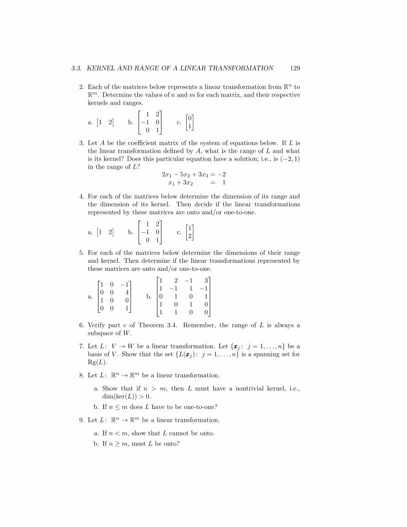
Example 4. Given the three points (1,−6), (2,0), and (3,6), we know from theabove discussion that there is a polynomial ppp(t), of degree 3− 1 = 2, such thatppp(1) = −6, ppp(2) = 0, and ppp(3) = 6. Find this polynomial.

Solution. The transformation L : P2 → R3 defined by the abscissas of thesethree points satisfies

L(111) = (1, 1, 1) L(ttt) = (1, 2, 3) L(ttt2) = (1, 4, 9)

The matrix representation for this transformation is

A =

1 1 11 2 41 3 9

This matrix has rank equal to 3. We wish to find ppp(t) such that L(ppp) = (−6, 0, 6).In terms of the coefficients aj of ppp(t) = a0 + a1t + a2t

2, we want a solution tothe equation

A

a0a1a2

=

−606

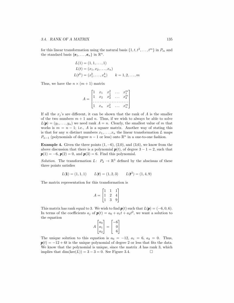
The unique solution to this equation is a0 = −12, a1 = 6, a2 = 0. Thus,ppp(t) = −12 + 6t is the unique polynomial of degree 2 or less that fits the data.We know that the polynomial is unique, since the matrix A has rank 3, whichimplies that dim(ker(L)) = 3− 3 = 0. See Figure 3.4. �


(2,0)

(3,6)

(1,−6)

p(t) = −12 + 6t

Figure 3.4

Problem Set 3.4

1. Calculate the rank of each of the following matrices:

a.[

1 0 1]

b.

101

c.

[

1 10 1

]

d.

1 1 11 0 11 1 11 0 −1

2. Calculate the rank of each of the following matrices:

a.[

1 2]

b.

1 2−1 00 1

c.

[

75

]

3. Each of the matrices below represents a linear transformation from Rn toRm. Determine the values of n and m for each matrix. Then determinethe dimensions of the range and kernel of L

a.

1 0 −10 0 41 0 00 0 1

b.

1 2 −1 31 −1 1 −10 1 0 11 0 1 01 1 0 0


4. For each matrix below, determine the dimensions of the range and kernel.Then decide if the linear transformation it represents is onto and/or one-to-one.

a.[

1 2]

b.

1 2−1 00 1

c.

[

75

]

5. For each matrix below determine the dimensions of the range and kernel.Then decide if the linear transformation it represents is onto and/or one-to-one.

a.

1 1 −15 0 42 1 01 1 1

b.

2 3 5 71 −1 1 −15 0 5 11 2 3 41 1 0 0

6. Compute the row rank and column rank of each of the following matrices:

a.

[

1 6 0 32 −1 1 0

]

b.

−3 6 4 12 8 4 3

−4 1 0 0

c.

1 2 14 5 68 −1 26 1 0

7. Consider the following system of linear equations:

2x1 − 6x3 = −6x2 + x3 = 1

Let A be the coefficient matrix of this system.

a. Compute the rank of A.

b. dim(ker(A)) =? Find a basis for ker(A).

c. dim(Rg(A)) =? Find a basis for Rg(A).

d. Is A a one-to-one linear transformation?

e. Is A onto?

f. Does the above system of equations have a solution? If yes, charac-terize the solution set in terms of the kernel of A and one particularsolution.

8. Let L : R3 → R

2 have the matrix representation

A =

[

−2 1 34 −1 0

]

Show that the range of L and the column space of A are the same subspaceof R2.


9. Consider the following system of linear equations:

4x1 + 2x3 + x4 = 02x1 − x2 + x3 + 3x4 = 1

−8x1 − 2x2 − 4x3 + 3x4 = 2

Let A be the coefficient matrix of this system.

a. Compute the rank of A.

b. dim(ker(A)) =? Find a basis for ker(A).

c. dim(Rg(A)) =? Find a basis for Rg(A).

d. Is A a one-to-one linear transformation?

e. Is A onto?

f. Does the above system of equations have a solution? If yes, charac-terize the solution set in terms of the kernel of A and a particularsolution.

10. Let xxxk for k = 1, 2, . . . , p be vectors in a vector space. Let V = S[xxx1, . . .,xxxp]. If c is any nonzero constant show that

a. V = S[cxxx1,xxx2, . . . ,xxxp].

b. V = S[xxx1, cxxx1 + xxx2, . . . ,xxxp].

The reader should note that the result proved in this problem is what isneeded to verify Theorem 3.6, the vectors then representing the rows orcolumns of a matrix.

11. Given data points (1,0) and (2,1), define L : P2 → R2 by L(ppp) = (ppp(1),ppp(2)). Here ppp = ppp(t) is any polynomial of degree 2 or less. Find the matrixrepresentation of L with respect to the standard bases in P2 and R

2. Showthat the rank of A equals 2. What does this say about fitting polynomialsof degree at most 2 through the data points (1,0) and (2,1)?

12. Let ppp be any polynomial in P2. Define L : P2 → R3 by L(ppp) = (ppp(−2), ppp(0),ppp(1)). Find the matrix representation A of L with respect to the standardbases in P2 and R

3. Show that A has rank equal to 3. What does this sayabout fitting polynomials of degree 2 or less through three points in theplane with x coordinates −2, 0, and 1?

13. Find a polynomial in P1, if possible, that fits the following data:

a (2,6), (3,6) b. (2,0), (−1, 4) c. (2,6), (3,6), (4,7)

14. Find a polynomial in P2, if possible, that fits the following data:

a. (−2, 6), (3,7) b. (−2, 6), (3,7), (4,7)c. (−2, 6), (3,7), (4,7), (5,8)


15. Let V = C[0, 1], the vector space of real-valued continuous functions de-fined on [0,1]. Define the mapping L by

L[fff ] =

[

fff(0)

2+ fff

(

1

2

)

+fff(1)

2

](

1

2

)

Thus, if fff(1) = sin t, we have L[fff ] = [(sin 0)/2 + sin 12 + (sin 1)/2](12 ).

This formula is just the trapezoid rule for the approximate evaluation ofintegrals over the interval [0,1] using the points 0, 1

2 , and 1.

a. Show that L is a linear transformation, after deciding of course whatW should be. Characterize the range and kernel of L.

b. Let L1[fff ] = L[fff ]−´ 1

0 fff(t)dt. Show that L1 is also a linear transfor-mation. How would you describe its kernel?

16. For each of the following matrices A compute the rank of A,AT , AAT ,and ATA. You should get rank ATA equals rank A and rank AAT equalsrank AT . Hence all four numbers are equal.

a.[

1 1 2]

b.

[

1 0 20 1 3

]

c.

[

1 −23 2

]

17. Let A be any m×n matrix. How are the row space of A and the range ofAT related?

18. Let x1, x2, and x3 be three different numbers.

a. Show rank

[

1 x11 x2

]

= 2.

b. Show rank

1 x1 x211 x2 x221 x3 x23

= 3.

Hint: The matrix in a is row equivalent to

[

1 x10 x2 − x1

]

.

19. Define L : P2 → R3 by L[ppp] = (ppp(x1), ppp(x2), ppp(x3)), where the xj ’s are alldifferent. Show that L is one-to-one and onto.

20. Let x1, x2, . . . , xn be n pairwise distinct numbers. Let

A =

1 x1 x21 . . . xn−11

1 x2 x22 . . . xn−12

. . . . . . . . . . . . . . . . . . . . . .1 xn x2n . . . xn−1

n

Show that rank A = n.


3.5 Change of Basis Formulas

In Section 3.3 we learned how to represent a linear transformation as a matrix,and in the last section we saw how the matrix can be used to tell us some factsabout the kernel and range of the linear transformation. Clearly the “simpler”the matrix representation the easier it is to understand the linear transforma-tion. Since Gaussian elimination is a method used to obtain a “simple” matrixrepresentation for a system of equations, we have already seen the utility offinding nice representations.

Once we have a fixed linear transformation, that maps a vector space V intoitself, the only variable in determining its matrix representation is our choice ofbasis.

Before studying how to pick such a basis (cf. Chapter 5), we need to learnhow the matrix representations of the same linear transformation with respect todifferent bases are related to each other. Thus, let L be a linear transformationfrom V into V , where dim(V ) = n. Let F = {fff j : j = 1, . . . , n} and G ={gggj : j = 1, . . . , n} be two bases of V . Let A = [ajk] be the matrix representationof L with respect to F and let B = [bjk] be the matrix representation of L withrespect to G. This means that the following equations hold:

L[fff j ] =

n∑

k=1

akjfffk (3.7)

L[gggj ] =

n∑

k=1

bkjgggk (3.8)

Let P = [pjk] be the change of basis matrix that satisfies [xxx]TG = P [xxx]TF , that is

fff j =

n∑

k=1

pkjgggk (3.9)

and if P−1 = [qjk], then

gggj =

n∑

k=1

qkjfffk (3.10)

We refer the reader to Theorem 2.11 and the material preceding it. ComputingL[fff j ], we have

L[fff j ] = L

[

n∑

k=1

pkjgggk

]

=

n∑

k=1

pkjL[gggk]

=

n∑

k=1

pkj

(

n∑

s=1

bskgggs

)

=

n∑

k=1

n∑

s=1

pkjbsk

(

n∑

m=1

qmsfffm

)

=n∑

m=1

(

n∑

k=1

n∑

s=1

(qmsbskpkj)

)

fffm

3.5. CHANGE OF BASIS FORMULAS 141

Comparing this expression with (3.7) and equating coefficients, we have

amj =

n∑

k=1

n∑

s=1

qmsbskpkj (3.11)

for m and j varying from 1 through n. However, the right-hand side of (3.11)is the m, j entry of the matrix P−1BP . Thus we have

A = P−1BP and B = PAP−1 (3.12)

A better way to remember how the matrix representations A and B are relatedis to utilize formulas (3.3), that is,

[L(xxx)]TF = A[xxx]TF [L(xxx)]TG = B[xxx]TG

Thus,

[L(xxx)]TG = P [L(xxx)]TF = P (A[xxx]TF )

= (PA)(P−1[xxx]TG) = (PAP−1)[xxx]TG

Hence, we must have B = PAP−1. The reader is referred to problem 11 inSection 2.6 for a justification of this last step.

Example 1. Let L be a linear transformation from R2 to R2 defined byL(x1, x2) = (2x1+x2, 3x1−2x2). Verify formulas (3.12) for F = {(1, 1), (−1, 2)}and G = {(−1,−1), (2, 0)}.Solution. Writing the vectors in F as linear combinations of the vectors in G,we have

(1, 1) = −(−1,−1) + 0(2, 0)

(−1, 2) = −2(−1,−1) +

(

−3

2

)

(2, 0)

Thus,

P =

[

−1 −20 − 3

2

]

P−1 =

[

−1 43

0 − 23

]

To determine A, we compute

L(1, 1) = (3, 1) =7

3(1, 1)− 2

3(−1, 2)

L(−1, 2) = (0,−7) = −7

3(1, 1)− 7

3(−1, 2)

Thus,

A =

[

73 − 7

3

− 23 − 7

3

]


To determine B, we compute

L(−1,−1) = (−3,−1) = (−1,−1)− (2, 0)

L(2, 0) = (4, 6) = −6(−1,−1)− (2, 0)

Thus,

B =

[

1 −6−1 −1

]

Computing P−1BP we have

[

−1 43

0 − 23

]

[

1 −6−1 −1

] [

−1 −20 − 3

2

]

=

[

73 − 7

3

− 23 − 7

3

]

= A

which is formula (3.12). �

Example 2. Let L : R4 → R4 be a linear transformation defined by

L(x1, x2, x3, x4) = (2x3 + x4,−3x1 + x2 − x4, x1 − x3 + 6x4, x2 − x3)

Let S be the standard basis ofR4 and letG = {(−1, 0, 1, 1), (0, 1,−1, 0), (0, 0, 1, 1),(1, 0, 1, 0)}. Find the matrix representations of L with respect to S, and thenG, by employing (3.12).

Solution. Let A be the matrix representation of L with respect to S. Byinspection we have

A =

0 0 2 1−3 1 0 −11 0 −1 60 1 −1 0

If P−1 is the change of basis matrix that satisfies [x]TS = P−1[x]TG then,

P−1 =

−1 0 0 10 1 0 01 −1 1 11 0 1 0

An easy computation gives us

P =

−1 1 1 −10 1 0 01 −1 −1 20 1 1 −1

Using (3.12), where B is the matrix representation of L with respect to the basis


G, we have

B = PAP−1

=

−1 1 1 −10 1 0 01 −1 −1 20 1 1 −1

0 0 2 1−3 1 0 −11 0 −1 60 1 −1 0

−1 0 0 10 1 0 01 −1 1 11 0 1 0

=

4 2 2 −12 1 −1 −3

−5 0 −3 37 0 5 −2

As a check on our computations we compute L(−1, 0, 1, 1) using the matrix B,and then compare this with our original definition of L. The vector (−1, 0, 1, 1)is the first vector in the basis G. Thus, the first column of B contains thecoordinates of L(−1, 0, 1, 1) with respect to the basis G. Hence,

L(−1, 0, 1, 1) = 4(−1, 0, 1, 1) + 2(0, 1,−1, 0)− 5(0, 0, 1, 1) + 7(1, 0, 1, 0)

= (3, 2, 4,−1)

This is exactly what we get when we compute L(−1, 0, 1, 1) directly. �

The preceding calculations have shown us that if L : V → V is a lineartransformation, and A and B are two matrix representations of L with respectto two different bases of V , then there is a matrix P such that A = P−1BP .

Definition 3.9. Let A and B be two n× n matrices. We say that A is similarto B, if there is a nonsingular matrix P such that A = P−1BP .

As we have seen, the matrix P is nothing more than the matrix relating two dif-ferent bases of our vector space. Moreover, we understand that similar matricesare just different matrix representations of the same linear transformation.

The change of basis discussion assumed that the linear transformation Lmapped V into V . What happens when L : V → W , and we change bases inV and W? Without going through the calculations, we state the appropriatetheorem.

Theorem 3.8. Let L : V →W be a linear transformation. Let F and F be twobases of V . Let G and G be two bases of W . Let A be the matrix representationof L using the bases F and G while B is the representation using the bases F

and G . Let P = [pjk] be the change of basis matrix that satisfies [xxx]TF

= P [xxx]TF .Let Q = [qjk] be the matrix that satisfies [yyy]T

G= Q[yyy]TG. Then

A = Q−1BP (3.13)

The reader should look at problem 9 at the end of this section for one method ofproving this result.


Problem Set 3.5

1. Let L : R2 → R2 be defined by L(x1, x2) = (2x1, 2x2). Let F = {(1,−1),(2, 5)}.

a. Find the matrix representation A of L with respect to the standardbasis S.

b. Let P be the change of basis matrix that satisfies [xxx]TF = P [xxx]TS . FindP and P−1.

c. Find the matrix representation B of L with respect to the basis Fby using (3.12).

2. Let A be any 2× 2 scalar matrix, that is

A =

[

c 00 c

]

= cI2

Let P be any 2 × 2 nonsingular matrix. Show that PAP−1 equals A; cf.problem 1.

3. Let L : R3 → R3. Let F = {(1, 2,−3), (1, 0, 0), (0, 1, 0)}. Suppose

A =

0 1 −22 1 05 0 1

is the matrix representation of L with respect to the basis F . Use (3.12)to find the matrix representation of L with respect to the standard basis;cf. problem 4 of Section 3.2.

4. Suppose A =

[

2 1−1 2

]

is the matrix representation of a linear transfor-

mation with respect to the standard basis. Let P =

[

0 11 0

]

and set

B = PAP−1. Then B can be thought of as the matrix representation ofL with respect to some other basis. What is this basis?

5. Let A,B, and C be three n× n matrices. Show that

a. A is similar to itself.

b. If A is similar to B, then B is similar to A.

c. If A is similar to B and B is similar to C, then A is similar to C.

6. Let A be any 2× 2 matrix. Show that if A is similar to I2, then A = I2.

7. Let F = {(1, 2), (1, 0)} and G = {(1,−1), (0, 1)}. Let L(x1, x2) = (x1 +x2, 2x1 − x2). Find the matrix representations of L with respect to basesF and G. Verify (3.12).


8. Let F = {(1, 0, 1), (0, 1, 1), (1, 1, 0)} andG = {(1, 0,−1), (−1, 1, 0), (0, 0, 1)}.Let L(x1, x2, x3) = (x1 + x2 + x3, x2 + x3, x3). Verify (3.12) for the abovebases and linear transformation L.

9. Prove Theorem 3.8. Hint: Use problem 11 in Section 2.6 and formula(3.3).

10. Let F1 =

{[

1 00 0

]

,

[

0 10 0

]

,

[

0 01 0

]

,

[

0 00 1

]}

Let F2 =

{[

0 11 1

]

,

[

1 01 1

]

,

[

1 10 1

]

,

[

1 11 0

]}

Let G1 =

{[

1 0 00 0 0

]

,

[

0 1 00 0 0

]

,

[

0 0 10 0 0

]

,

[

0 0 01 0 0

]

,

[

0 0 00 1 0

]

,

[

0 0 00 0 1

]}

Let G2 =

{[

0 1 11 1 1

]

,

[

1 0 11 1 1

]

,

[

1 1 01 1 1

]

,

[

1 1 10 1 1

]

,

[

1 1 11 0 1

]

,

[

1 1 11 1 0

]}

Let jAk be the matrix representation of a linear transformation L : M22 →M23 with respect to the bases Gj and Fk. That is,

[L(xxx)]TGj= jAk[xxx]

TFk

Suppose that

1A1 =

−2 0 −3 01 0 1 00 1 4 13 1 −5 02 −2 0 11 2 3 4

Find the other three matrix representations.

11. Suppose A and B are similar n×n matrices, i.e., there is a matrix P suchthat A = PBP−1.

a. How are ker(A) and ker(B) related?

b. How are Rg(A) and Rg(B) related?

12. Let L : P2 → P2 be a linear transformation. Let F = {t2+t−1, t2+2, t−6}.Suppose the matrix representation of L with respect to F is

A =

−14 −2 −1823 11 1811 2 15

Find the matrix representation of L with respect to the standard basis ofP2.


Supplementary Problems

1. Define and give examples of each of the following:

a. Linear transformation

b. Range and kernel of a linear transformation

c. Rank of a matrix

d. Column (row) rank

2. Let A =

2 61 −23 5

be the matrix representation of a linear transformation

from Rk to RP .

a. k =?p =?

b. Determine the dimensions of ker(A) and Rg(A).

3. For each of the following matrices determine the rank and find a basis forthe kernel:

a.

3 1 21 0 1

−1 1 1

b.

−1 2 0 64 3 −1 01 0 0 1

c.

4 2 4 66 3 6 92 1 2 1

4. Let A and B be two matrices. Show that

Rank(AB) ≤ minimum{rank(A),rank(B)}

Hint: Rank (A) equals dim(Rg(A)).

5. Define L : R2 → R2 by L(x1, x2) = (x1 + x2,−x2). Show that L mapsthe straight line y = mx onto the straight line y = −[m/(m+1)]x. Whathappens to the line y = −x?

6. Describe, geometrically, the following linear transformations, and in eachcase determine the kernel and range:

a. L(x1, x2) = (x1 − x2, x1 + x2)

b. L(x1, x2) = (2x1 − x2, 4x1 − 2x2)

7. Let V1, V2, and V3 be vector spaces with bases F1, F2, and F3, respectively.Suppose L1 : V1 → V2 and L2 : V2 → V3 are linear transformations. LetA1 and A2 be their corresponding matrix representations with respect tothe given bases. Define L : V1 → V3 by L(xxx) = L2(L1(xxx)).

a Show that L is a linear transformation from V1 to V3.

b. Show that the matrix representation of L with respect to the basesF1 and F3 is A2A1.


8. A linear transformation L : R2 → R

2 is said to be positive if it mapsthe first quadrant into the first quadrant; that is, if x1 and x2 are bothpositive, then so are y1 and y2, where L(x1, x2) = (y1, y2).

a. Let L(x1, x2) = (ax1+ bx2, cx1+dx2). Show that L is positive if andonly if a, b, c, and d are all non-negative and at least one of {a, b} ispositive and one of {c, d} is positive.

b. Find a positive linear transformation whose matrix representationwith respect to some basis has at least one negative entry.

c. Find an example of a positive linear transformation whose kernel hasdimension equal to 1.

9. A mapping T from a vector space V into V is said to be an affine trans-formation if

T (xxx) = L(xxx) + aaa

where L is a linear transformation from V into V and a is any fixed vectorin V .

a. Show that T (xxx) = L(xxx) + aaa is a linear transformation if and only ifa equals the zero vector.

b. Given any straight line in R2, show that there is an affine transfor-

mation that maps the line x2 = 0 onto the given line. Hint: Rotateand then translate.

10. Two vector spaces V1 and V2 are said to be isomorphic if there is a lineartransformation L : V1 → V2 that is both one-to-one and onto.

a. Suppose dim(V1) = m and V1 is isomorphic to V2. Show dim(V2) =m.

b. Show that two finite-dimensional vector spaces are isomorphic if andonly if they have the same dimension.

c. Let V1 = R1 and let V2 be the vector space defined in Example 5

Section 2.2. Define L : V1 → V2 by L(x) = ex. Show that L is alinear transformation that is one-to-one and onto.

11. Let V = {∑nk=1 ak sin(kx)e

−k2t, n any positive integer and ak arbitrarynumbers}.

a. Under ordinary addition and multiplication show that V is a vector

space. Define L : V → V by L[u] = ∂u∂t − ∂2u

∂x2 .

b. Show L is a linear transformation.

c. Find the kernel and range of L.


12. If V is a finite-dimensional space and L is a linear transformation from Vinto V , then L is one-to-one if and only if L is onto. This result, as thefollowing shows, may not be true if V is infinite-dimensional. Let V bethe vector space of all polynomials in the variable t.

a. Define L[ppp](t) = tppp(t). Thus, L[ttt] = ttt2, L[ttt2] = ttt3, and L[tttn] = tttn+1.Show that L is one-to-one but not onto.

b. Define L[ppp](t) = ppp′(t). Thus, L[tttn] = ntttn−1. Show that L is onto butnot one-to-one. What is the kernel of L?

13. Let L be a linear transformation from V into V . A subspace W of V issaid to be invariant under L if, for every xxx in W , L[xxx] is also in W . Thus,we may also consider L to be a linear transformation fromW toW . Showthat for any linear transformation L each of the following is an invariantsubspace:

a. W = {0},W = V .

b. For any constant λ, show Wλ = {xxx : L[xxx] = λx} is an invariantsubspace.

14. Let A =

2 1 0−2 3 00 0 4

be the matrix representation of a linear transfor-

mation L with respect to the standard basis. Show that S[eee1] is not aninvariant subspace but that S[eee1, eee2] and S[eee3] are invariant subspaces; cf.problem 13.

15. Let F = {xxx1, . . . ,xxxn} be a basis for a vector space V . Let L be a lineartransformation from V into V for which S[xxx1, . . . ,xxxk] and S[xxxk+1, . . . ,xxxn]are both invariant subspaces of L. Let A be the matrix representation ofL with respect to the basis F . Show that

A =

[

B1 00 B2

]

where B1 is a k×k matrix and B2 is an (n−k)×(n−k) matrix. Conversely,suppose that A has the above form. Show that the above two subspacesmust be invariant.

linear transformation.pdf

Documents

Transcript of linear transformation.pdf