
Linear Static Analysis of a Plate with Hole · PDF fileLinear Static Analysis of a Plate with...
25
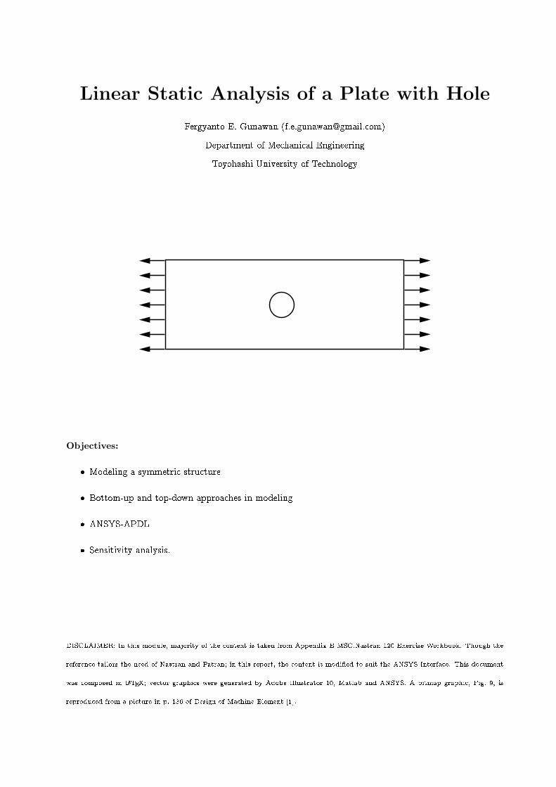
Linear Static Analysis of a Plate with Hole Objectives:
Transcript of Linear Static Analysis of a Plate with Hole · PDF fileLinear Static Analysis of a Plate with...
Linear Static Analysis of a Plate with Hole
Fergyanto E. Gunawan ([email protected])
Department of Mechanical Engineering
Toyohashi University of Technology
Objectives:
� Modeling a symmetric structure
� Bottom-up and top-down approaches in modeling
� ANSYS-APDL
� Sensitivity analysis.
DISCLAIMER: In this module, majority of the content is taken from Appendix E MSC.Nastran 120 Exercise Workbook. Though the
reference tailors the need of Nastran and Patran; in this report, the content is modi�ed to suit the ANSYS Interface. This document
was composed in LATEX; vector graphics were generated by Adobe Illustrator 10, Matlab and ANSYS. A bitmap graphic, Fig. 9, is
reproduced from a picture in p. 136 of Design of Machine Element [1].
Linear Static Analysis of a Plate with Hole
Model Description:
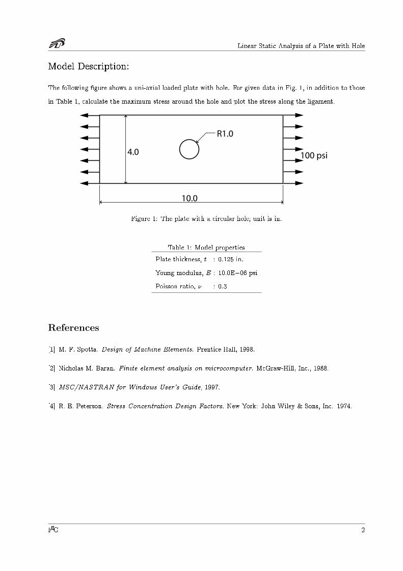
The following �gure shows a uni-axial loaded plate with hole. For given data in Fig. 1, in addition to those
in Table 1, calculate the maximum stress around the hole and plot the stress along the ligament.
10.0
4.0
R1.0
100 psi
Figure 1: The plate with a circular hole; unit is in.
Table 1: Model properties
Plate thickness, t : 0.125 in.
Young modulus, E : 10.0E+06 psi
Poisson ratio, � : 0.3
References
[1] M. F. Spotts. Design of Machine Elements. Prentice Hall, 1998.
[2] Nicholas M. Baran. Finite element analysis on microcomputer. McGraw-Hill, Inc., 1988.
[3] MSC/NASTRAN for Windows User's Guide, 1997.
[4] R. E. Peterson. Stress Concentration Design Factors. New York: John Wiley & Sons, Inc. 1974.
FEG 2
Linear Static Analysis of a Plate with Hole
Pre-Processing Phase:
CREATE A NEW FOLDER
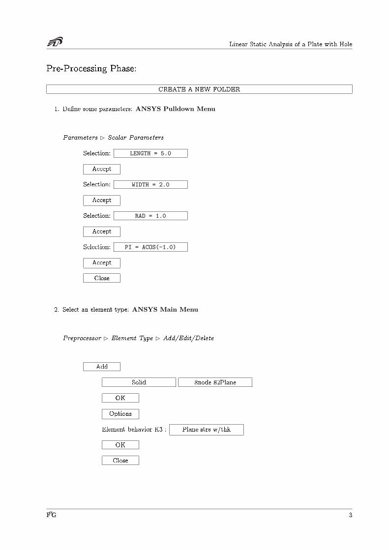
1. De�ne some parameters: ANSYS Pulldown Menu
Parameters B Scalar Parameters
Selection: LENGTH = 5.0
Accept
Selection: WIDTH = 2.0
Accept
Selection: RAD = 1.0
Accept
Selection: PI = ACOS(-1.0)
Accept
Close
2. Select an element type: ANSYS Main Menu
Preprocessor B Element Type B Add/Edit/Delete
Add
Solid 8node 82Plane
OK
Options
Element behavior K3 : Plane strs w/thk
OK
Close
FEG 3
Linear Static Analysis of a Plate with Hole
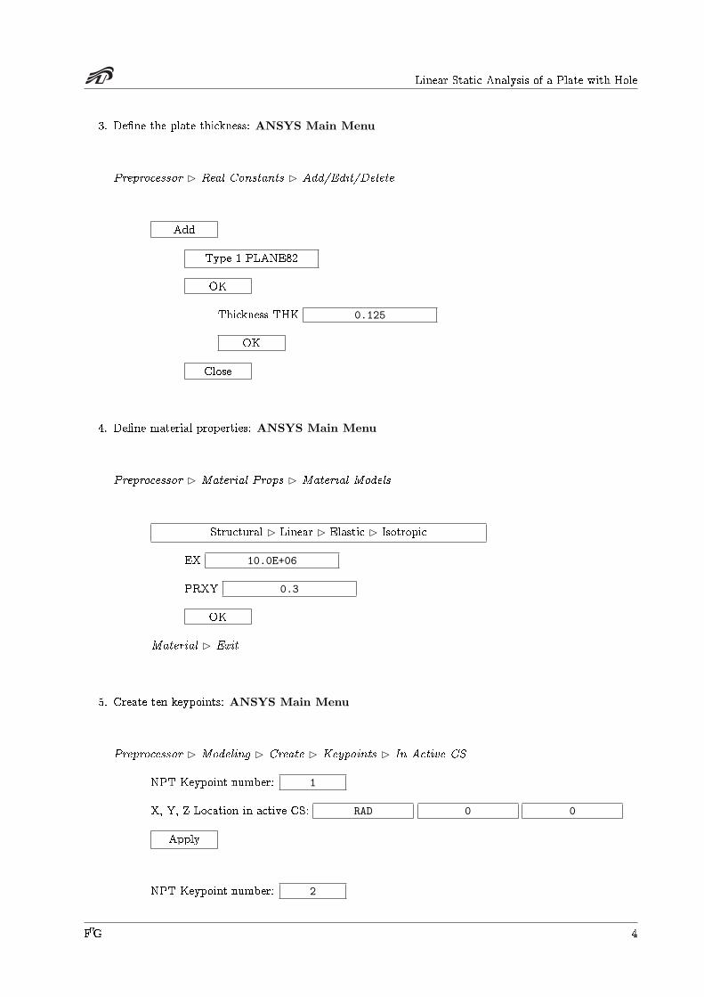
3. De�ne the plate thickness: ANSYS Main Menu
Preprocessor B Real Constants B Add/Edit/Delete
Add
Type 1 PLANE82
OK
Thickness THK 0.125
OK
Close
4. De�ne material properties: ANSYS Main Menu
Preprocessor B Material Props B Material Models
Structural B Linear B Elastic B Isotropic
EX 10.0E+06
PRXY 0.3
OK
Material B Exit
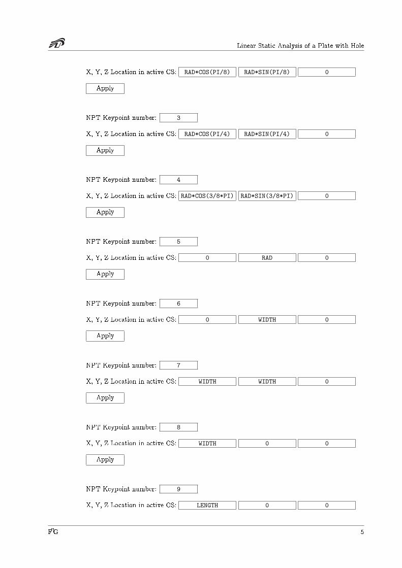
5. Create ten keypoints: ANSYS Main Menu
Preprocessor B Modeling B Create B Keypoints B In Active CS
NPT Keypoint number: 1
X, Y, Z Location in active CS: RAD 0 0
Apply
NPT Keypoint number: 2
FEG 4
Linear Static Analysis of a Plate with Hole
X, Y, Z Location in active CS: RAD*COS(PI/8) RAD*SIN(PI/8) 0
Apply
NPT Keypoint number: 3
X, Y, Z Location in active CS: RAD*COS(PI/4) RAD*SIN(PI/4) 0
Apply
NPT Keypoint number: 4
X, Y, Z Location in active CS: RAD*COS(3/8*PI) RAD*SIN(3/8*PI) 0
Apply
NPT Keypoint number: 5
X, Y, Z Location in active CS: 0 RAD 0
Apply
NPT Keypoint number: 6
X, Y, Z Location in active CS: 0 WIDTH 0
Apply
NPT Keypoint number: 7
X, Y, Z Location in active CS: WIDTH WIDTH 0
Apply
NPT Keypoint number: 8
X, Y, Z Location in active CS: WIDTH 0 0
Apply
NPT Keypoint number: 9
X, Y, Z Location in active CS: LENGTH 0 0
FEG 5
Linear Static Analysis of a Plate with Hole
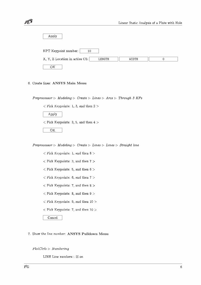
Apply
NPT Keypoint number: 10
X, Y, Z Location in active CS: LENGTH WIDTH 0
OK
6. Create lines: ANSYS Main Menu
Preprocessor B Modeling B Create B Lines B Arcs B Through 3 KPs
< Pick Keypoints: 1, 3, and then 2 >
Apply
< Pick Keypoints: 3, 5, and then 4 >
OK
Preprocessor B Modeling B Create B Lines B Lines B Straight line
< Pick Keypoints: 1, and then 8 >
< Pick Keypoints: 3, and then 7 >
< Pick Keypoints: 5, and then 6 >
< Pick Keypoints: 6, and then 7 >
< Pick Keypoints: 7, and then 8 >
< Pick Keypoints: 8, and then 9 >
< Pick Keypoints: 9, and then 10 >
< Pick Keypoints: 7, and then 10 >
Cancel
7. Show the line number: ANSYS Pulldown Menu
PlotCtrls B Numbering
LINE Line numbers : � on
FEG 6

Linear Static Analysis of a Plate with Hole
OK
Plot B Lines
You should see a model similar to that in Fig. 2. In the next steps, we will create three areas; those
areas are surrounded by lines, for Area 1: L2, L4, L6, L5; for Area 2: L1, L3, L7, L4; and for Area 3:
L7, L8, L9, L10.
Figure 2: Model of plate with hole having line numbers turned on.
8. Create three areas: ANSYS Main Menu
Preprocessor B Modeling B Create B Areas B Arbitrary B By Lines
< Pick lines: L2, L4, L6, and then L5 >
Apply
< Pick lines: L1, L3, L7, and then L4 >
Apply
< Pick lines: L7, L8, L9, and then L10 >
FEG 7
Linear Static Analysis of a Plate with Hole
OK
9. Control the mesh density: ANSYS Main Menu
Preprocessor B Meshing B MeshTool
Lines : Set
< Pick lines: 1, 2, 3, 4, 5, 6, 7, and then 9 >
Apply
NDIV No. of element divisions 4
Apply
< Pick lines: 7 and 9 >
NDIV No. of element divisions 6
Ok
10. Show the area number: ANSYS Pulldown Menu
PlotCtrls B Numbering
AREA Area numbers : � on
OK
Plot B Areas
11. Mesh the model: ANSYS Main Menu
Preprocessor B Meshing B MeshTool
Shape : � Quad
Shape : � Mapped
Mesh
< Pick areas: A1, A2, and then A3 >
FEG 8

Linear Static Analysis of a Plate with Hole
NDIV = 4
PLANE42 PLANE82
PLANE42 PLANE82
Figure 3: MeshTool of ANSYS and some of its functionality.
OK
FEG 9
Linear Static Analysis of a Plate with Hole
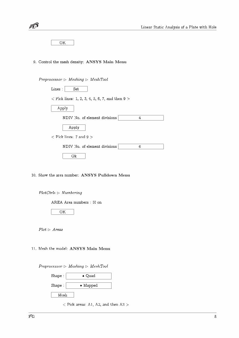
Figure 4: The plate with hole model having area numbers turned on.
Important note I The results, especially the stress, of a �nite element analysis strongly depends on the
mesh. Concerning the mesh, Nicholas M. Baran [2] suggests followings:
Mesh Transition: You can use a tringle or control the mesh spacing ratio. However,
in using the mesh spacing ratio, keep l2 � 2l1 and l4 � 2l3.
l1l2
l3
l4
Element Aspect Ratio: Aspect ratio (l=w) should be kept less than 3, if possible.
w
l
w
l
Excessiveaspect ratio
Element Skewness: Try to keep the skew angle, �, less than 30 degrees. Nastran
issues a warning if the angle is greater than 30 degrees [3].
θ
FEG 10
Linear Static Analysis of a Plate with Hole
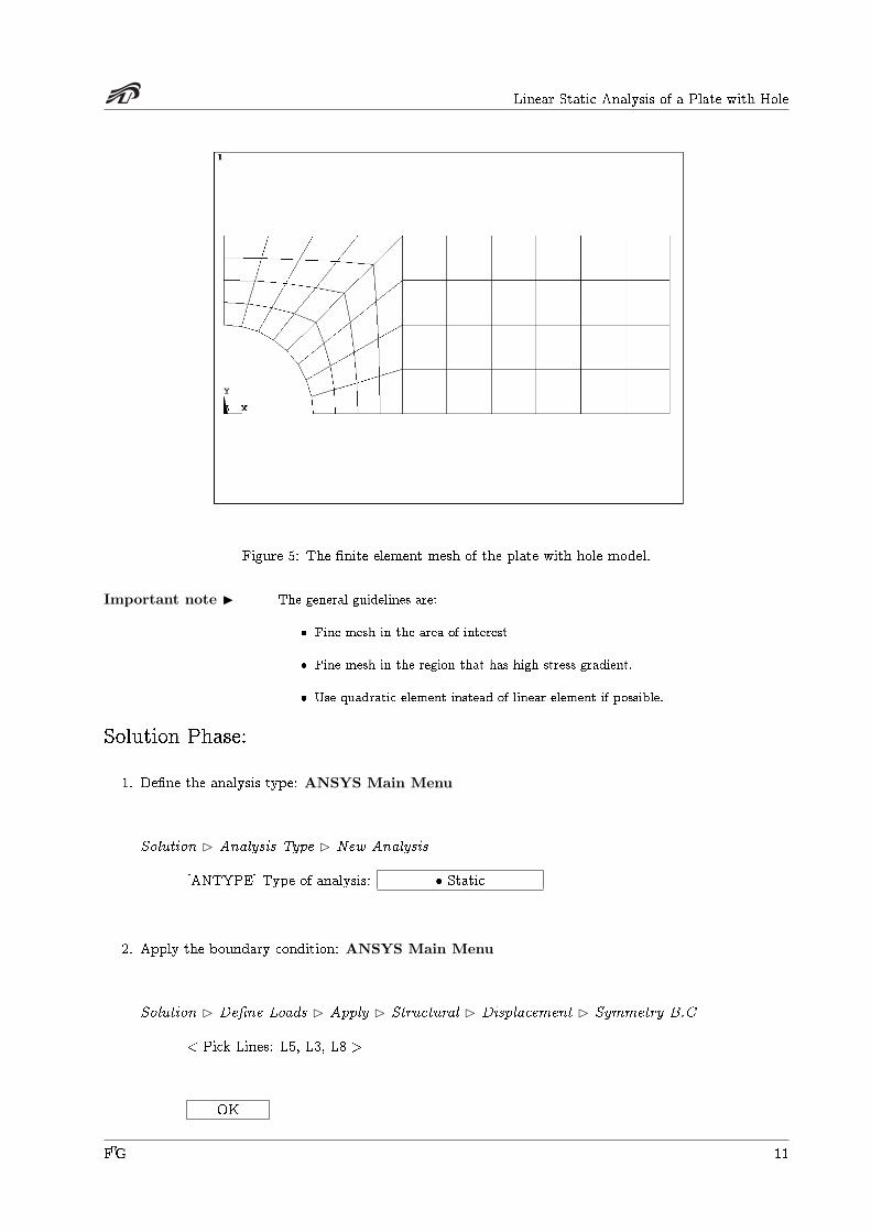
Figure 5: The �nite element mesh of the plate with hole model.
Important note I The general guidelines are:
� Fine mesh in the area of interest
� Fine mesh in the region that has high stress gradient.
� Use quadratic element instead of linear element if possible.
Solution Phase:
1. De�ne the analysis type: ANSYS Main Menu
Solution B Analysis Type B New Analysis
[ANTYPE] Type of analysis: � Static
2. Apply the boundary condition: ANSYS Main Menu
Solution B De�ne Loads B Apply B Structural B Displacement B Symmetry B.C
< Pick Lines: L5, L3, L8 >
OK
FEG 11

Linear Static Analysis of a Plate with Hole
Important Notes I Following �gures show several types of symmetry structures:
(a) Axial Symmetry (b) Planar Symmetry
(c) Cyclic Symmetry (d) Repetitive Symmetry
However, the symmetricalness does not only about the geometry, but also the constraints
and the loading conditions. For an example, see following:
Symmetry point
Anti-symmetry point
3. Apply uniform stress: ANSYS Main Menu
Solution B De�ne Loads B Apply B Structural B Pressure B On Lines
< Pick Line: L9 >.
OK
VALUE Load PRES: -1.0
OK
4. Solve the problem: ANSYS Main Menu
Solution B Solve B Current LS
OK
Close
FEG 12
Linear Static Analysis of a Plate with Hole
Post Processing Phase:
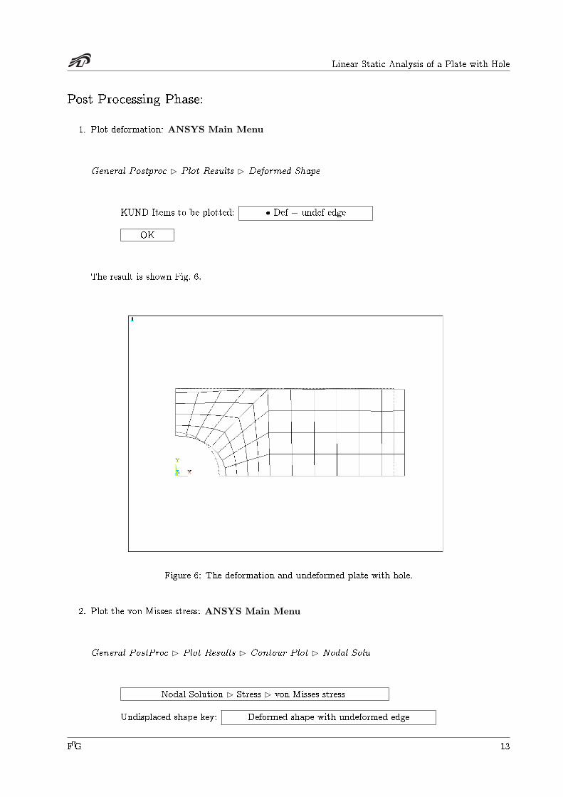
1. Plot deformation: ANSYS Main Menu
General Postproc B Plot Results B Deformed Shape
KUND Items to be plotted: � Def + undef edge
OK
The result is shown Fig. 6.
Figure 6: The deformation and undeformed plate with hole.
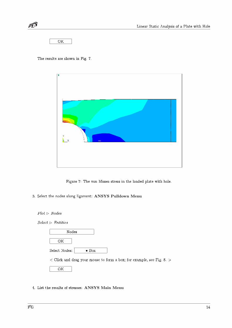
2. Plot the von Misses stress: ANSYS Main Menu
General PostProc B Plot Results B Contour Plot B Nodal Solu
Nodal Solution B Stress B von Misses stress
Undisplaced shape key: Deformed shape with undeformed edge
FEG 13
Linear Static Analysis of a Plate with Hole
OK
The results are shown in Fig. 7.
Figure 7: The von Misses stress in the loaded plate with hole.
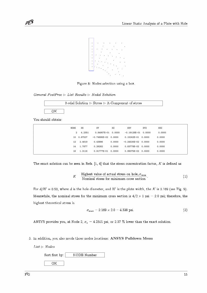
3. Select the nodes along ligament: ANSYS Pulldown Menu
Plot B Nodes
Select B Entities
Nodes
OK
Select Nodes: � Box
< Click and drag your mouse to form a box; for example, see Fig. 8. >
OK
4. List the results of stresses: ANSYS Main Menu
FEG 14
Linear Static Analysis of a Plate with Hole
Figure 8: Nodes selection using a box.
General PostProc B List Results B Nodal Solution
Nodal Solution B Stress B X-Component of stress
OK
You should obtain:
NODE SX SY SZ SXY SYZ SXZ
2 4.2351 0.84957E-01 0.0000 -0.19128E-01 0.0000 0.0000
10 0.67527 -0.74895E-02 0.0000 0.15242E-01 0.0000 0.0000
12 2.4619 0.43886 0.0000 -0.24530E-02 0.0000 0.0000
14 1.7877 0.28282 0.0000 0.83778E-02 0.0000 0.0000
16 1.3116 0.91777E-01 0.0000 0.99075E-02 0.0000 0.0000
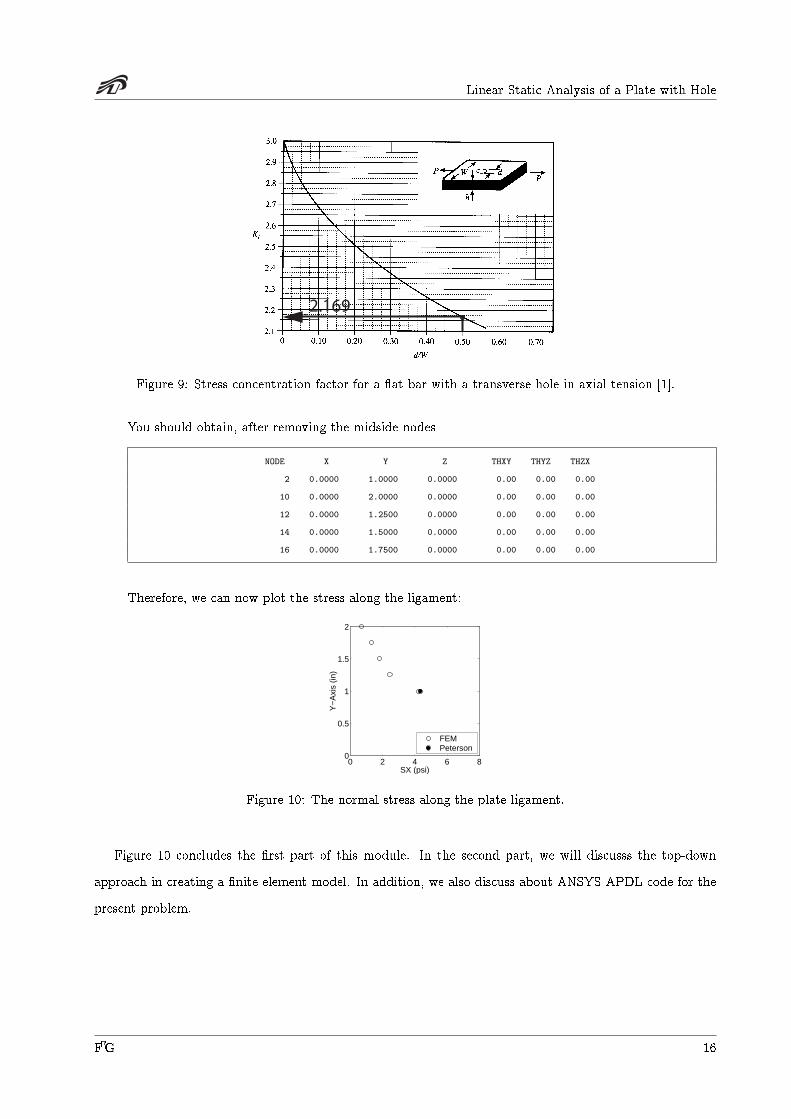
The exact solution can be seen in Refs. [1, 4] that the stress concentration factor, K is de�ned as
K =Highest value of actual stress on hole; �max
Nominal stress for minimum cross section: (1)
For d=W = 0:50, where d is the hole diameter, and W is the plate width, the K is 2.169 (see Fig. 9).
Meanwhile, the nominal stress for the minimum cross section is 4=2 � 1 psi = 2.0 psi; therefore, the
highest theoretical stress is
�max = 2:169� 2:0 = 4:338 psi: (2)
ANSYS provides you, at Node 2, �x = 4.2351 psi, or 2.37 % lower than the exact solution.
5. In addition, you also needs those nodes locations: ANSYS Pulldown Menu
List B Nodes
Sort �rst by: NODE Number
OK
FEG 15
Linear Static Analysis of a Plate with Hole
2.169
Figure 9: Stress concentration factor for a at bar with a transverse hole in axial tension [1].
You should obtain, after removing the midside nodes
NODE X Y Z THXY THYZ THZX
2 0.0000 1.0000 0.0000 0.00 0.00 0.00
10 0.0000 2.0000 0.0000 0.00 0.00 0.00
12 0.0000 1.2500 0.0000 0.00 0.00 0.00
14 0.0000 1.5000 0.0000 0.00 0.00 0.00
16 0.0000 1.7500 0.0000 0.00 0.00 0.00
Therefore, we can now plot the stress along the ligament:
0 2 4 6 80
0.5
1
1.5
2
Y−
Axi
s (in
)
SX (psi)
FEMPeterson
Figure 10: The normal stress along the plate ligament.
Figure 10 concludes the �rst part of this module. In the second part, we will discusss the top-down
approach in creating a �nite element model. In addition, we also discuss about ANSYS-APDL code for the
present problem.
FEG 16
Linear Static Analysis of a Plate with Hole
Top-down Modeling Approach
Two approachs in modeling:
Bottom-up approach: keypoints I lines I area I volume I meshing
Top-down approach: primitives I boolean operations I meshing
We study the top-down approach in this section. In the next section, the APDL code also will be based on
the present log �le.
CREATE A NEW FOLDER
Pre-Processing Phase:
1. Select element type, de�ne the thickness, and also de�ne material properties. Repeat the previous
pre-processing phase, the �rst four steps.
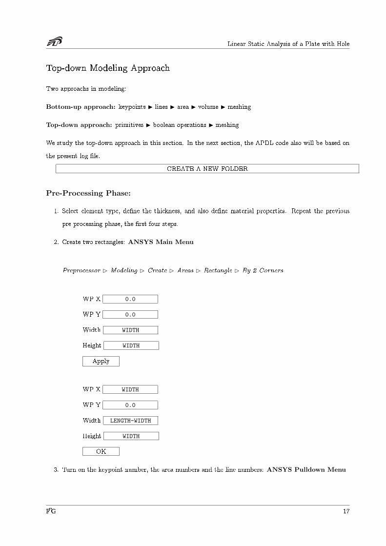
2. Create two rectangles: ANSYS Main Menu
Preprocessor B Modeling B Create B Areas B Rectangle B By 2 Corners
WP X 0.0
WP Y 0.0
Width WIDTH
Height WIDTH
Apply
WP X WIDTH
WP Y 0.0
Width LENGTH-WIDTH
Height WIDTH
OK
3. Turn on the keypoint number, the area numbers and the line numbers: ANSYS Pulldown Menu
FEG 17

Linear Static Analysis of a Plate with Hole
PlotCtrls B Numbering
KEYPOINT Keypoint numbers: � On
AREA Area Numbers � On
LINE Line numbers � On
OK
4. Create a circle: ANSYS Main Menu
Preprocessor B Modeling B Create B Area B Circl B Solid Circle
WP X 0.0
WP Y 0.0
Radius RAD
OK
5. Substract Area A1 to Area A3: ANSYS Main Menu
Preprocessing B Modeling B Operate B Booleans B Substract B Areas
< Pick Area A1 >
OK
< Pick Area A3 >
OK
You should see the new area which has a number of A4
6. Merges coincident Keypoints: ANSYS Main Menu
Preprocessor B Numbering B Ctrls B Merge Items
FEG 18

Linear Static Analysis of a Plate with Hole
Label Type of item to be merge Keypoints
OK
7. Create a keypoint: ANSYS Main Menu
Preprocessing B Modeling B Create B Keypoints B In Active CS
NPT Keypoint number 100
X, Y, Z Location in active CS 0.0 0.0 0.0
8. Create a line: ANSYS Main Menu
Preprocessing B Modeling B Create B Lines B Lines B Strainght Line
< Pick Node 100 and 8 >
OK
OK
9. Cut the area into two areas: ANSYS Main Menu
Preprocessing B Modeling B Operate B Booleans B Divide B Area by Line
< Pick Area A4 >
OK
< Pick Line L1 >
OK
You should obtain A1, A2, and A3
10. Merges coincident Keypoints: ANSYS Main Menu
FEG 19
Linear Static Analysis of a Plate with Hole
Preprocessor B Numbering B Ctrls B Merge Items
Label Type of item to be merge Keypoints
OK
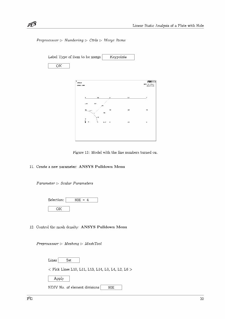
Figure 11: Model with the line numbers turned on.
11. Create a new parameter: ANSYS Pulldown Menu
Parameter B Scalar Parameters
Selection: NOE = 4
OK
12. Control the mesh density: ANSYS Pulldown Menu
Preprocessor B Meshing B MeshTool
Lines Set
< Pick Lines L10, L11, L13, L14, L3, L4, L2, L6 >
Apply
NDIV No. of element divisions NOE
FEG 20

Linear Static Analysis of a Plate with Hole
Apply
< Pick Lines 5, and 7 >
Apply
NDIV No. of element divisions NOE*3/2
OK
Shape Quad
Shape Mapped
Mesh
< Pick Area A1, A2, A3 >
OK
Close
See the previous solution phase.
Mesh Sensitivity Study
The stress depends on the mesh in a �nite element analysis; although, physically it should not. To study
how the stress depend on the mesh, we perform a mesh sensitivity study. In this study, we analyse the
structure for a number of the mesh-size. In short, we change NOE, and see how it a�ect the maximum �x.
The important lines from your log �le are reproduced following.
1 *SET,LENGTH,5
2 *SET,WIDTH,2
3 *SET,RAD,1
4 *SET,PI,ACOS(-1.0)
5 /PREP7
6 ET,1,PLANE82
7 KEYOPT,1,3,3
8 KEYOPT,1,5,0
9 KEYOPT,1,6,0
10 R,1,0.125,
11
12 MPTEMP,,,,,,,,
13 MPTEMP,1,0
14 MPDATA,EX,1,,10E6
15 MPDATA,PRXY,1,,0.3
FEG 21
Linear Static Analysis of a Plate with Hole
16
17 BLC4,0,0,WIDTH,WIDTH
18 BLC4,WIDTH,0.0,LENGTH-WIDTH,WIDTH
19 CYL4,0.0,0.0,RAD
20 ASBA, 1, 3
21 K,100,0.0,0.0,0.0,
22 LSTR, 100, 3
23 ASBL, 4, 1
24 NUMMRG, KP
25 *SET,NOE,4
26 LESIZE,_Y1, , ,NOE, , , , ,1
27 LESIZE,_Y1, , ,NOE*3/2, , , , ,1
28 MSHAPE,0,2D
29 MSHKEY,1
30 AMESH,_Y1
31 FINISH
32 /SOL
33 ANTYPE,0
34 DL,P51X, ,SYMM
35 SFL,P51X,PRES,-1.0,
36 SOLVE
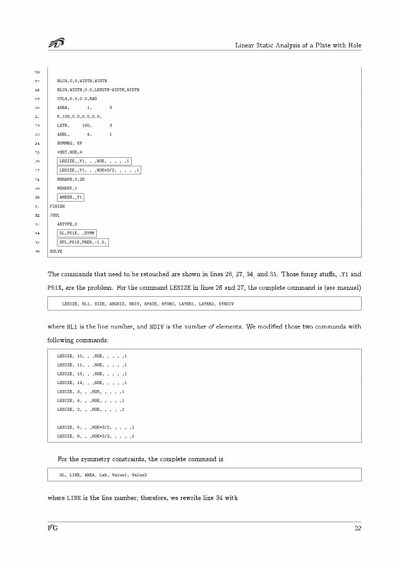
The commands that need to be retouched are shown in lines 26, 27, 34, and 35. Those funny stu�s, Y1 and
P51X, are the problem. For the command LESIZE in lines 26 and 27, the complete command is (see manual)
LESIZE, NL1, SIZE, ANGSIZ, NDIV, SPACE, KFORC, LAYER1, LAYER2, KYNDIV
where NL1 is the line number, and NDIV is the number of elements. We modi�ed those two commands with
following commands:
LESIZE, 10, , ,NOE, , , , ,1
LESIZE, 11, , ,NOE, , , , ,1
LESIZE, 13, , ,NOE, , , , ,1
LESIZE, 14, , ,NOE, , , , ,1
LESIZE, 3, , ,NOE, , , , ,1
LESIZE, 4, , ,NOE, , , , ,1
LESIZE, 2, , ,NOE, , , , ,1
LESIZE, 5, , ,NOE*3/2, , , , ,1
LESIZE, 6, , ,NOE*3/2, , , , ,1
For the symmetry constraints, the complete command is
DL, LINE, AREA, Lab, Value1, Value2
where LINE is the line number; therefore, we rewrite line 34 with
FEG 22
Linear Static Analysis of a Plate with Hole
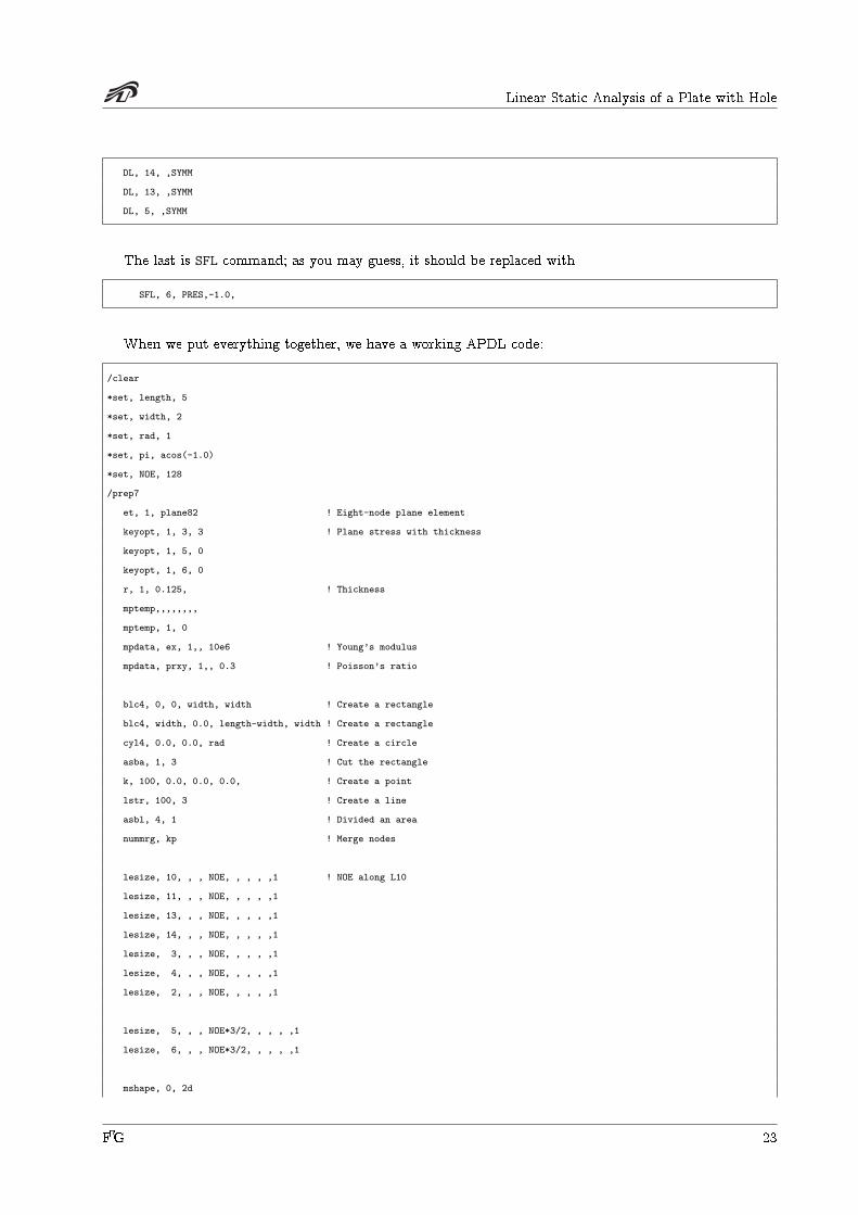
DL, 14, ,SYMM
DL, 13, ,SYMM
DL, 5, ,SYMM
The last is SFL command; as you may guess, it should be replaced with
SFL, 6, PRES,-1.0,
When we put everything together, we have a working APDL code:
/clear
*set, length, 5
*set, width, 2
*set, rad, 1
*set, pi, acos(-1.0)
*set, NOE, 128
/prep7
et, 1, plane82 ! Eight-node plane element
keyopt, 1, 3, 3 ! Plane stress with thickness
keyopt, 1, 5, 0
keyopt, 1, 6, 0
r, 1, 0.125, ! Thickness
mptemp,,,,,,,,
mptemp, 1, 0
mpdata, ex, 1,, 10e6 ! Young’s modulus
mpdata, prxy, 1,, 0.3 ! Poisson’s ratio
blc4, 0, 0, width, width ! Create a rectangle
blc4, width, 0.0, length-width, width ! Create a rectangle
cyl4, 0.0, 0.0, rad ! Create a circle
asba, 1, 3 ! Cut the rectangle
k, 100, 0.0, 0.0, 0.0, ! Create a point
lstr, 100, 3 ! Create a line
asbl, 4, 1 ! Divided an area
nummrg, kp ! Merge nodes
lesize, 10, , , NOE, , , , ,1 ! NOE along L10
lesize, 11, , , NOE, , , , ,1
lesize, 13, , , NOE, , , , ,1
lesize, 14, , , NOE, , , , ,1
lesize, 3, , , NOE, , , , ,1
lesize, 4, , , NOE, , , , ,1
lesize, 2, , , NOE, , , , ,1
lesize, 5, , , NOE*3/2, , , , ,1
lesize, 6, , , NOE*3/2, , , , ,1
mshape, 0, 2d
FEG 23
Linear Static Analysis of a Plate with Hole
mshkey, 1
amesh, 1 ! Mesh Area 1
amesh, 2 ! Mesh Area 2
amesh, 3 ! Mesh Area 3
finish
/sol
antype, 0 ! Static analysis
dl, 14, ,symm ! Symmetric constraints
dl, 13, ,symm !
dl, 5, ,symm !
sfl, 6, pres,-1.0, ! Apply uniform tensile stress
solve ! Solve
finish
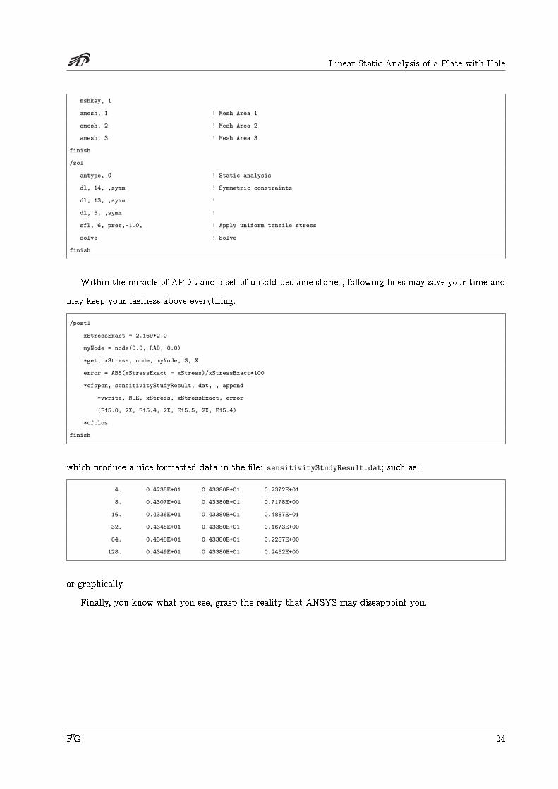
Within the miracle of APDL and a set of untold bedtime stories, following lines may save your time and
may keep your laziness above everything:
/post1
xStressExact = 2.169*2.0
myNode = node(0.0, RAD, 0.0)
*get, xStress, node, myNode, S, X
error = ABS(xStressExact - xStress)/xStressExact*100
*cfopen, sensitivityStudyResult, dat, , append
*vwrite, NOE, xStress, xStressExact, error
(F15.0, 2X, E15.4, 2X, E15.5, 2X, E15.4)
*cfclos
finish
which produce a nice formatted data in the �le: sensitivityStudyResult.dat; such as:
4. 0.4235E+01 0.43380E+01 0.2372E+01
8. 0.4307E+01 0.43380E+01 0.7178E+00
16. 0.4336E+01 0.43380E+01 0.4887E-01
32. 0.4345E+01 0.43380E+01 0.1673E+00
64. 0.4348E+01 0.43380E+01 0.2287E+00
128. 0.4349E+01 0.43380E+01 0.2452E+00
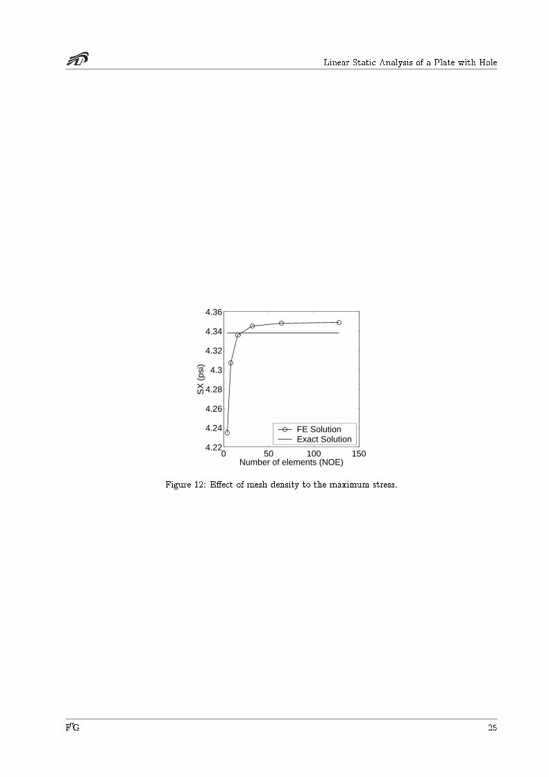
or graphically
Finally, you know what you see, grasp the reality that ANSYS may dissappoint you.
FEG 24
Linear Static Analysis of a Plate with Hole
0 50 100 1504.22
4.24
4.26
4.28
4.3
4.32
4.34
4.36
Number of elements (NOE)
SX
(ps
i)
FE SolutionExact Solution
Figure 12: E�ect of mesh density to the maximum stress.
FEG 25


