1

Linear Programming

Learning Goals.

Introduce Linear Programming Problems.

Widget Example, Graphical Solution.

Basic Theory:

• Feasible Set, Vertices, Existence of Solutions.

• Equivalent formulations.

Outline of Simplex Method.

Runtimes for Linear Program Solvers.

Readings: Read text section 11.6, and sections 1 and 2 of Tom Ferguson’s notes (see course homepage).

2

Widget Factory Example

A factory makes x1 (thousand) widgets of type 1 and x2 of type 2.

Total profit for making x = (x1, x2)T is:

profit = x1 + 2x2

Due to a limited resource (e.g. time) we require:

x1 + x2 ≤ 4

Two waste products from making widget 1 are required for widget 2. So we need to make enough of widget 1 to supply the construction of widget 2. These constraints are:

-x1 + x2 ≤ 1-3x1 + 10x2 ≤ 15

Finally, both x1 and x2 must be non-negative.

How many widgets of each type should be made to maximize profit?

3

Linear Programming: Standard Form

Consider a real-valued, unknown, n-vector x = (x1, x2, … , xn)T.

A linear programming problem in standard form (A, b, c) has the three components:

Objective Function: We wish to choose x to maximize:cT x = c1x1 + c2x2 + … cnxn

with x subject to the following constraints:

Problem Constraints: For an m x n matrix A, and an m x 1 vector b:A x ≤ b

Non-negativity Constraints:x ≥ 0

Constants:A an m x n matrix,b an m x 1 vector,c an n x 1 vector.

Linear function of x

Linear inequality constraints on x

Notation: For two K-vectors x and y, x ≤ y iff xk ≤ yk for each k = 1, 2, …, K.Other inequalities (≥, etc.) defined similarly.

4

Widget Factory Example: Continued.

Pose Widget problem as a linear program in Standard Form.Need to specify constants, (A, b, c).

Unknowns: x = (x1, x2)T number (in thousands) of the two widget types.

Objective function (profit): cT x = c1x1 + c2x2 = x1 + 2x2, so cT = (c1, c2) = (1, 2).

Problem Constraints: A x ≤ b

so

Non-negativity Constraints:x ≥ 0

5

Graphing the Widget Factory Example

Linear Program specified by (A, b, c).

x1

x2

1 2 3 4

1 -

2 -

3 -

cTx = 2

cTx = 4

Objective Function: cTx, c = (1, 2)T

cTx increases indirection c.

Mixtures of widgetswith the same profit

6

Graphing the Widget Factory Example

Example: x = (x1, x2)T. Linear Program specified by (A, b, c).

x1

x2

1 2 3 4

1 -

2 -

3 -

Objective Function: cTx, c = (1, 2)T

Non-negativity: x ≥ 0. Feasible Set

Problem Constraints: Ax ≤ b,

Half-plane:x1 + x2 ≤ 4

Half-plane:-x1 + x2 ≤ 1

Half-plane:-3x1 + 10x2 ≤ 15

7

Graphing the Widget Factory Example

Example: x = (x1, x2)T. Linear Program specified by (A, b, c).

x1

x2

1 2 3 4

1 -

2 -

3 -

Objective Function: cTx, c = (1, 2)T

Non-negativity: x ≥ 0.

Problem Constraints: Ax ≤ b,

Direction of increasing profit.

8

Graphing the Widget Factory Example

Example: x = (x1, x2)T. Linear Program specified by (A, b, c).

x1

x2

1 2 3 4

1 -

2 -

3 -

Objective Function: cTx, c = (1, 2)T

Non-negativity: x ≥ 0.

Problem Constraints: Ax ≤ b,

Max profit: cTx

9

Graphing the Widget Factory Example

Example: x = (x1, x2)T. Linear Program specified by (A, b, c).

x1

x2

1 2 3 4

1 -

2 -

3 -

Objective Function: cTx, c = (1, 2)T

Non-negativity: x ≥ 0.

Optimal Solution:xT = (25, 27)/13

Problem Constraints: Ax ≤ b,

10

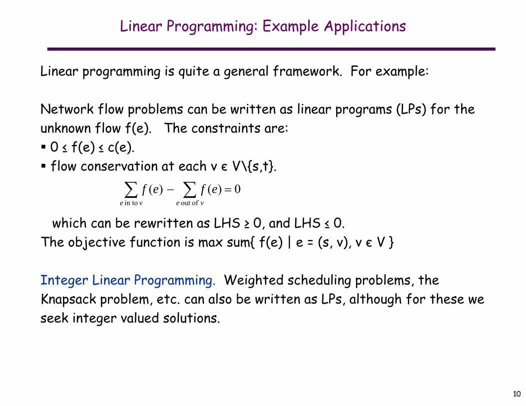
Linear Programming: Example Applications

Linear programming is quite a general framework. For example:

Network flow problems can be written as linear programs (LPs) for the unknown flow f(e). The constraints are: 0 ≤ f(e) ≤ c(e). flow conservation at each v є V\{s,t}.

which can be rewritten as LHS ≥ 0, and LHS ≤ 0.The objective function is max sum{ f(e) | e = (s, v), v є V }

Integer Linear Programming. Weighted scheduling problems, the Knapsack problem, etc. can also be written as LPs, although for these we seek integer valued solutions.

0)()( ofout in to

veve

efef

11

Linear Programming Theory: Feasible Set

Given the constants (A, b, c), consider the linear program:Objective Function: Maximize cT x, where x = (x1, x2, … , xn)T.Problem Constraints: A x ≤ b Non-negativity Constraints: x ≥ 0

Define the feasible set F = { x | Ax ≤ b and x ≥ 0 }.F could be empty (no solutions to all the constraints).

F is a convex polytope. (A region of defined by the intersection of finitely many half-spaces, e.g., ak

T x ≤ bk and xj ≥ 0.)

Convexity of F: Let u, v є F, and let s є [0, 1]. Then su + (1-s)v є F.

Pf: u, v є F implies Au ≤ b and Av ≤ b. So A [su + (1-s)v ] = s Au + (1-s)Av ≤ sb + (1-s)b = b, for s є [0, 1]. A similar argument shows su + (1-s)v ≥ 0. Therefore su + (1-s)v є F.

[Rn

12

Example Feasible Set

x1

x2

1 2 3 4

1 -

2 -

3 -

Feasible Set

Half-plane:x1 + x2 ≤ 4

Half-plane:-x1 + x2 ≤ 1

Half-plane:-3x1 + 10x2 ≤ 15

13

Example Feasible Set

x1

x2

1 2 3 4

1 -

2 -

3 -

Feasible Set

Half-plane:x1 + x2 ≤ 4

Half-plane:-x1 + x2 ≤ 1

Half-plane:3x1 - 10x2 ≤ -15

14

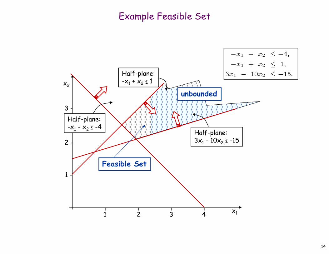
Example Feasible Set

x1

x2

1 2 3 4

1 -

2 -

3 -

Feasible Set

Half-plane:-x1 - x2 ≤ -4

Half-plane:-x1 + x2 ≤ 1

Half-plane:3x1 - 10x2 ≤ -15

unbounded

15

Linear Programming Theory: Characterization of a Vertex

What’s a vertex of the feasible set?

Let P be the (m+n) x n matrix and p the (m+n)-vector which represents both the problem and non-negativity constraints:

Let s = {s1, s2, … , sn} be a selection of n row numbers, 1 ≤ si ≤ m+n. Define Q(s) to be the n x n matrix formed from the s-rows of P, and q(s) the n-vector formed from the same rows of p.

Defn: A point v є is a vertex of the feasible set F iff there exists an s such that:

Q(s) is nonsingular, v = [Q(s)]-1 q(s), i.e., v satisfies the n equalities selected by s, and v є F, i.e., v is feasible.

See 2D examples above, and 3D example next.

[Rn

16

Three Dimensional Example: Vertices

x1

x2

x3

Problem Constraints: x1 + 3x3 ≤ 600x2 + x3 ≤ 300

x1 + x2 + x3 ≤ 400x2 ≤ 250

Vertex is a soln of:x1 + 3x3 = 600x2 + x3 = 300

x1 + x2 + x3 = 400

Feasible set F isthis closed polytope.

Vertex is a soln of:x1 + 3x3 = 600

x1 + x2 + x3 = 400x2 = 0

Vertex: Choose n = 3 problem or non-negativity constraints, solve equalities for v:

17

Linear Programming Theory: Characterization of a Solution

Given the constants (A, b, c), consider the linear program:Objective Function: Maximize cT x, where x = (x1, x2, … , xn)T, c ≠ 0.Problem Constraints: A x ≤ b Non-negativity Constraints: x ≥ 0

Define: Feasible set F = { x | A x ≤ b and x ≥ 0 }

Theorem: The linear program above either:1. has no solution, in which case either

• the feasible set F is empty, or• the objective cTx unbounded (and F is unbounded),

2. has a solution x*.In case 2, x* can be taken to be a vertex of the polytope F (theremay also be non-vertex solutions x є F with cTx = cTx*)

See examples.

18

Solution at Vertex: Example 1

x1

x2

1 2 3 4

1 -

2 -

3 -

Feasible Set

Half-plane:x1 + x2 ≤ 4

Half-plane:-x1 + x2 ≤ 1

Half-plane:-3x1 + 10x2 ≤ 15

Optimal solutionat vertex.

19

Solution at Vertex: Example 2

x1

x2

1 2 3 4

1 -

2 -

3 -

Feasible Set

Half-plane:x1 + x2 ≤ 4

Half-plane:-x1 + x2 ≤ 1

Half-plane:-3x1 + 10x2 ≤ 15

Optimal solutionat vertex.

20

Solution along Closed Segment: Example

x1

x2

1 2 3 4

1 -

2 -

3 -

Feasible Set

Half-plane:x1 + x2 ≤ 4

Half-plane:-x1 + x2 ≤ 1

Optimal solutions at vertices and along segment between.

c must be “special” forsuch a case to occur.

Half-plane:-3x1 + 10x2 ≤ 15

21

Three Dimensional Example

x1

x2

x3

Problem Constraints: x1 + 3x3 ≤ 600x2 + x3 ≤ 300

x1 + x2 + x3 ≤ 400x2 ≤ 250

Maximize cTx,cT = (2, 3, 4),Feasible set F is

this closed polytope.

Multiple solns iff c is perpendicularto an edge or faceof F.

Colours indicate value of cTx.Larger cTx → hotter colours.

22

Variations in the Formulation of Linear Programs

A given LP can be expressed in many equivalent forms.

Given an LP in standard form, with constants (A, b, c).

Some alternatives: minimize –cTx equivalent to maximizing cTx. Constraint aTx ≤ b equivalent to -aTx ≥ -b Constraint aTx = b iff aTx ≤ b and –aTx ≤ -b. Ax ≤ b iff Ax + z = b and z ≥ 0, with “slack variables” z = (z1, … , zm)T. min|e| can be rewritten as min(e+ + e- ) with the linear constraint

e = e+ - e- and the non-negativity constraint e+, e- ≥ 0.

These alternatives are useful for posing problems as LPs in standard form, or reposing LPs in alternative forms useful for computation.

23

A Sketch of the Simplex Method

Simplex method: Given an LP in standard form (A, b, c). Let P and p be:

Let v be a feasible vertex. So v = v(s), where s = {s1, …, sn} denotes a set of n “selected” rows of P v ≤ p, such that Q(s) v = q(s) and Q(s) is nonsingular (see the defn. of a vertex, above).while true *

Consider each neighbour s’ of s (i.e., s’ and s differ only inone element.).

Choose an edge v(s) to v(s’) s.t. the objective increases.If there is no such edge, v(s) is a solution. Stop.If there is an edge leaving v(s) on which the objective is unbounded,

then there is no solution to this LP. Stop.Set s ← s’, v ← v’(s’)

end* Modulo non-cycling conditions

24

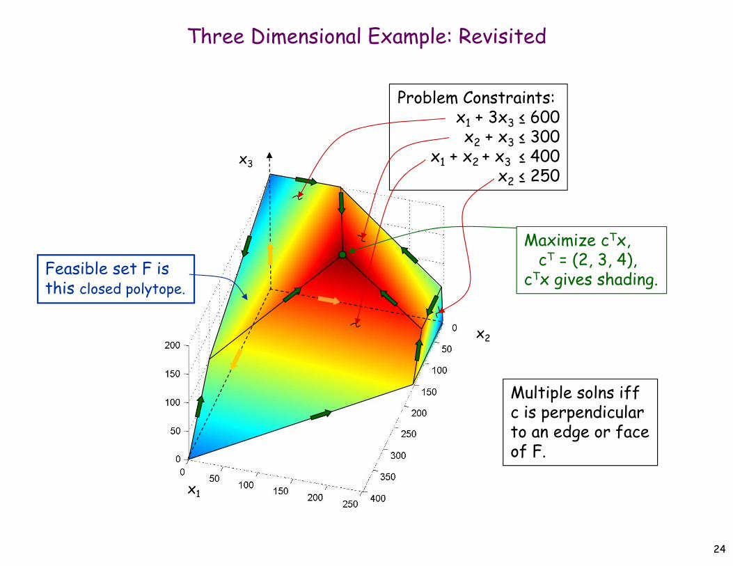
Three Dimensional Example: Revisited

x1

x2

x3

Problem Constraints: x1 + 3x3 ≤ 600x2 + x3 ≤ 300

x1 + x2 + x3 ≤ 400x2 ≤ 250

Maximize cTx,cT = (2, 3, 4),

cTx gives shading.Feasible set F isthis closed polytope.

Multiple solns iff c is perpendicularto an edge or faceof F.

25

Pivoting

The step from v(s) to v(s’) is called pivoting.

One row of Pv ≤ p is dropped from s, and it is replaced by another row to form s’.

The selection of a pivot is guaranteed not to decrease the objective function.

If some care is taken to avoid cycling, the Simplex Algorithm is guaranteed to converge to a solution after finitely many pivot steps.

In an efficient implementation, each pivot step costs O((m+n)n) real number operations.

Unfortunately, simplex may visit exponentially many vertices in contrived cases. E.g., number of choices for s, (n+m) choose n.

26

Obtaining an Initial Vertex

We need an initial feasible vertex to start the Simplex Algorithm.

Given the LP constants (A, b, c), consider the start-up LP:Objective Function: Maximize -z1 - … -zm, where z = (z1, z2, … , zm)T.

Equivalent to minimizing z1 + … +zm

Problem Constraints: A x - z ≤ b, Non-negativity Constraints: x, z ≥ 0

For this start-up LP we have the initial guess, x = 0, z = b- where bk-=-bk

if bk < 0 and 0 otherwise.

This start-up LP has a solution (x0, 0) (i.e., with z = 0 and the objective function equal to 0) iff x0 is a feasible solution of the original LP.

Simplex will return a feasible vertex x0 on this start-up LP, so long as the original feasible set F is not empty.

27

Runtime for Simplex Algorithm

Worst case runtime is exponential. The Simplex Algorithm might visit exponentially many vertices as m and n grow.

In practice:

the method is highly efficient,

typically requires a number of steps which is just a small multiple ofthe number of variables.

LPs with thousands or even millions of variables are routinely solvedusing the simplex method on modern computers.

efficient, highly sophisticated implementations are available.

28

Runtimes for Linear Programming Solvers

Interior point methods provided the first polynomial time algorithms known for LP.

These iterate through the interior of the feasible set F.

Ellipsoid algorithm, Khachiyan, 1979. Interior point projective method, Karmarkar, 1984.

Interior point methods are now generally considered competitive with the simplex method in most, though not all, applications.

Sophisticated software packages are available.

Integer Linear Programming (ILP): An LP problem but with the added constraint that the solution vector x must be integer valued. ILP is NP-hard.