Inequalities and linear · PDF fileCHAPTER9 Inequalities and linear programming What is a...

P1: FXS/ABE P2: FXS0521672600Xc09.xml CUAU034-EVANS March 11, 1904 1:36

C H A P T E R

9Inequalities and linear

programming

What is a linear inequality?

How do we solve linear inequalities?

What is linear programming and how is it used?

In Chapter 3, ‘Linear graphs and models’, you learned how linear equations and their graphs

are used to model practical situations, such as plant growth, service charges and flow problems.

In this chapter you will learn how linear inequalities and their graphs can be used to model a

different set of practical situations, such as determining the mix of products in a supermarket

to maximise profit, or designing a diet to provide maximum nutrition for minimum cost.

This is known as linear programming. Linear programming requires you to solve both linear

equations and linear inequalities. You learned how to solve linear equations in Chapter 2,

‘Linear relations and equations’. You now need to learn how to solve linear inequalities.

9.1 Linear inequalities in one variableLinear inequalities in one variable and the number lineAn expression such as 9 ≤ 3x ≤ 21 is called a linear inequality in one variable. It is an

inequality, not an equation, because it involves an inequality sign (≤) rather than an equals

sign ( = ). The sign ‘ ≤ ’ means ‘less than or equal to’.

The solution to the linear equation 3x = 9 is x = 3, and the solution to the linear equation

3x = 21 is 7.

We can represent these solutions on a number line by putting a closed circle (•) on the number

line at x = 3 and x = 7 as shown.

x = 3 x = 7

–2 –1 0 1 3 4 5 6 7 8 92–3x

When solving an inequality and graphing its solution on a number line, we need to be careful

about whether the end values of the solution are included in the range of possible values.

376Cambridge University Press • Uncorrected Sample Pages • 978-0-521-74049-4 2008 © Evans, Lipson, Jones, Avery, TI-Nspire & Casio ClassPad material prepared in collaboration with Jan Honnens & David Hibbard

SAMPLE

Back to Menu >>>


Chapter 9 — Inequalities and linear programming 377

End values includedTo solve the linear inequality

9 ≤ 3x ≤ 21

we divide through by 3 and get

9

3≤ 3x

3≤ 21

3or 3 ≤ x ≤ 7

There is no single solution to this inequality. Any value of x from 3 to 7 is a solution. For

example, x = 3, x = 3.5, x = 4.95 and x = 7 are all possible solutions. In fact, it is

impossible to list every possible solution, as there are an infinite number of solutions.

However, we can represent all the possible solutions on a number line.

This is done by marking the points x = 3 and x = 7 with a closed circle (•) on the number

line. These points are then joined by drawing a solid line to indicate that all the values between

x = 3 and x = 7 are also solutions, as shown below.

–2 –1 0 1 3 4 5 6 7 8 92–3x

3 ≤ x ≤ 7

End values not includedTo solve the linear inequality

9 < 3x < 21

we divide through by 3 to obtain the solution

3 < x < 7

The sign ‘ < ’ means ‘less than’. This means that x = 3 and x = 7 are not solutions, but all

values between x = 3 and x = 7 are possible solutions.

To represent this solution on a number line, mark in the points x = 3 and x = 7 with an

open circle (◦). These two open circles are then joined by a solid line to indicate that all the

values between 3 and 7 are solutions, but not x = 3 and x = 7.

–2 –1 0 1 3 4 5 6 7 8 92–3x

3 < x < 7

Note that 7 > x > 3 represents the same values of x as 3 < x < 7.

A gallery of signs= as in a = b reads as ‘a equals b’

> as in a > b reads as ‘a is greater than b’

≥ as in a ≥ b reads as ‘a is greater than or equal to b’

< as in a < b reads as ‘a is less than b’

≤ as in a ≤ b reads as ‘a is less than or equal to b’

Cambridge University Press • Uncorrected Sample Pages • 978-0-521-74049-4 2008 © Evans, Lipson, Jones, Avery, TI-Nspire & Casio ClassPad material prepared in collaboration with Jan Honnens & David Hibbard

SAMPLE

Back to Menu >>>


378 Essential Standard General Mathematics

Example 1 Solving an inequality and graphing the solution

Solve the inequality

−10 < 5x ≤ 40

for x and display the solution on a number line.

Solution

1 Write the inequality. −10 < 5x ≤ 40

2 Solve the inequality for x by dividing through by 5. or−10

5<

5x

5≤ 40

53 Display the solution on a number line. or − 2 < x ≤ 8

� Draw a number line to include −2 and 8.–2 –1 0 1 3 4 5 6 7 8 92–3

x

� Mark the point x = −2 with an open

circle.–2 –1 0 1 3 4 5 6 7 8 92–3

x

� Mark the point x = 8 with a closed

circle.–2 –1 0 1 3 4 5 6 7 8 92–3

x

� Join the two points with a solid line.–2 –1 0 1 3 4 5 6 7 8 92–3

x

� Write in the solution inequality on

the graph.–2 –1 0 1 3 4 5 6 7 8 92–3

x–2 < x ≤ 8

Example 2 Solving an inequality and graphing the solution

Solve the inequality

10x > 20

for x and display the solution on a number line.

Solution

1 Write the inequality. 10x > 20

2 Solve the inequality for x by dividing through by 10. or10x

10>

20

103 Display the solution on a number line. or x > 2

� Draw a number line to include 2.–2 –1 0 1 3 4 5 6 7 8 92–3

x

� Mark in the point x = 2 with an open

circle.–2 –1 0 1 3 4 5 6 7 8 92–3

x

� To indicate all values of x greater than 2,

draw a solid line from this point to the

right that potentially goes on forever.

–2 –1 0 1 3 4 5 6 7 8 92–3x

� Write in the solution inequality on the

graph. –2 –1 0 1 3 4 5 6 7 8 92–3x

x > 2


SAMPLE

Back to Menu >>>



Linear inequalities in one variable and the coordinate planeWe can also represent linear inequalities in one

variable on the coordinate plane.

If the equation x = 3 is plotted on a set of axes we

will have a vertical straight line, located at x = 3.

O

(3, 6)

(3, 3)

x

(3, –1)

x =

3

y

(3, 0)

While the value of y changes along the line, for

every point on this line the value of x is 3.

Just as with graphing the solution of an inequality on

a number line, we need to be careful about whether the

boundary lines (end values) of the solution are included

in the range of possible values.

Boundary line includedIf we tried to plot the inequality x ≥ 3, we would have

to plot all the points in the plane that have an x-value

greater than or equal to 3.

O

(5, 6)

x(4, –1)

x =

3

y

x > 3

(3, 0)

Required region

Of course we cannot show each individual point.

What we do is shade in the region containing these

points. The shaded region starts at the vertical line

x = 3 and extends right forever.

Some representative points that satisfy the condition

x ≥ 3, and which are found in the shaded region, have

also been plotted.

Boundary line not includedThe plot of the inequality x > 3 is similar to the plot of

x ≥ 3, but the line x = 3 is drawn as a dashed line to

indicate that it is not included in the region.

O

(5, 6)

x(4, –1)

x =

3

y

Required region

x > 3Some representative points that satisfy the condition

x > 3 have also been plotted.

Note: For (5, 6), 5 > 3(4, −1), 4 > 3

Therefore both points satisfy the inequality x > 3.

Example 3 Plotting a linear inequality in one variable on the coordinate plane

On the coordinate plane, plot the graphs of:

a y ≤ 4

b −1 < y < 3


SAMPLE

Back to Menu >>>



Solution

a y ≤ 4

1 Draw in a solid line y = 4 to define the boundary

of the shaded region.

2 Shade the region on and below the line y = 4 to

represent all the points defined by y ≤ 4.

x

y

(0, 4)

y < 4

O

y = 4

b −1 < y < 3

1 Draw in a dashed line y = 3 to define the upper boundary

of the shaded region.

2 Draw in a dashed line y = −1 to define the lower

boundary of the shaded region.

3 Shade the region between the lines y = 3 and y = −1 to

represent all the points defined by −1 < y < 3.

x

y

O

(0, –1)

–1 < y < 3

(0, 3)

y = –1

y = 3

Exercise 9A

1 Which of the symbols <, = or > should be placed in the box in each of the following?

a 7 9 b 3 2 c 7 + 1 9 − 1 d 0.5 1

e 8 4 f −3 1 g −2 − 1 h 0 0.5

2 Represent each of the following inequalities on a number line.

a 1 ≤ x ≤ 4 b 0 < x < 4 c x < 4

d x ≥ 4 e −1 ≤ x < 4 f 3 < x ≤ 5

3 Write down an inequality represented by each of the following graphs.

a–2 –1 0 1 3 4 5 6 7 82

xb

–2 –1 0 1 3 4 5 6 7 82x

c–2 –1 0 1 3 4 5 6 7 82

xd

–2 –1 0 1 3 4 5 6 7 82x

e–2 –1 0 1 3 4 5 6 7 82

x

4 Solve each of the following inequalities and represent its solution on a number line.

a 3x ≥ 15 b 20x < 100 c 2x > −4

d 9x ≥ 36 e −12 ≤ 6x < 24 f 10 < 5x ≤ 25

5 A person becomes a teenager when they turn 13. They stop being a teenager when they turn

20. Let x be the variable age (in years).


SAMPLE

Back to Menu >>>



a Write down an inequality in terms of x that defines a teenager.

b Graph this inequality on a number line.

6 Carry-on luggage in most passenger aircraft can

weigh no more than 5 kg. Let x be the variable

weight (in kg).

a Write down an inequality in terms of x that

defines the acceptable weight for carry-on

luggage.

b Graph this inequality on a number line.

7 Graph the following inequalities on the coordinate plane.

a x ≤ 1 b x > −2 c y ≤ 5

d y > 1 e x < 2 f −2 ≤ y ≤ 2

g −1 < x < 2 h 3 < x ≤ 5 i −3 ≤ y < 0

9.2 Linear inequalities in two variablesThe inequalities

y − x > 2 y − x ≥ 2

y − x < 2 y − x ≤ 2

are linear inequalities in two variables, x and y.

x

y

2

2

4

4

–2–2

–4

6

8

10

0

(2, 8)

(4, 4)(2, 4)

y – x

= 2

To help us interpret these inequalities, we

have drawn the graph of y − x = 2. This line

(red) separates the coordinate plane into two

regions.

The line y – x = 2The line is defined by the equation y − x = 2 and coloured red. It includes all the points that

lie on the line.

From the graph above we can see that the point (2, 4) lies on the line. The points (2, 8) and

(4, 4) clearly do not lie on the line.


SAMPLE

Back to Menu >>>



We can also show this by carrying out the following tests, using the equation of the line.

Test:

(2, 4): y − x = 4 − 2 = 2; so the point (2, 4) lies on the line y − x = 2.

(2, 8): y − x = 8 − 2 = 6; 6 is greater than 2, so (8, 9) does not lie on y − x = 2.

(4, 4): y − x = 4 − 4 = 0; 0 is less than 2, so (4, 4) does not lie on the line y − x = 2.

The regions y – x > 2 and y – x ≥≥≥≥≥≥≥≥≥≥≥≥≥≥≥≥≥≥≥ 2This region is defined by the inequality y − x > 2 and coloured light blue. It includes all the

points that lie above the line; the point (2, 8) is an example.

By including the line in this region, we have a

way of representing the inequality

y − x ≥ 2

This region includes all the points on and above

the line.

From the graph on the right we can see that� the points (2, 4) and (2, 8) are examples of

points that lie in this region.

x

y

2

2

4

4

–2–2

–4

6

8

10

0

(2, 8)

(4, 4)(2, 4)

y − x

= 2

� the point (4, 4) clearly does not lie in the

region.

We can also show this by carrying out the

following tests, using the equation of the line.

Test:

(2, 4): y − x = 4 − 2 = 2; so the point (2, 4) lies in the region y − x ≥ 2.

(2, 8): y − x = 8 − 2 = 6; 6 is greater than 2, so the point (2, 8) lies in the region y − x ≥ 2

(4, 4): y − x = 4 − 4 = 0; 0 is less than 2, so (4, 4) does not lie in the region y − x ≥ 2.

The regions y – x < 2 and y – x ≤≤≤≤≤≤≤≤≤≤≤≤≤≤≤≤≤≤ 2This region is defined by the inequality y − x < 2 and coloured purple. It includes all the

points that lie below the line; the point (4, 4) is an example.

By including the line in this region, we have a

way of representing the inequality

y − x ≤ 2

This region includes all the points on and below

the line.

From the graph on the right we can see that� the points (2, 4) and (4, 4) are examples of

points that lie in this region.

x

y

2

2

4

4

–2–2

–4

6

8

10

0

(2, 8)

(4, 4)(2, 4)

y – x

= 2

� the point (2, 8) clearly does not lie in the

region.


SAMPLE

Back to Menu >>>



We can also show this by carrying out the following tests using the equation of the line.

Test:

(2, 4): y − x = 4 − 2 = 2; so the point (2, 4) lies in the region y − x ≤ 2.

(2, 8): y − x = 8 − 2 = 6; 6 is greater than 2, so (8, 9) does not lie in the region y − x ≤ 2.

(4, 4): y − x = 4 − 4 = 0; 0 is less than 2, so (4, 4) lies in the region y − x ≤ 2.

We now have a graphical way of representing inequalities.

Linear inequalities can be represented by regions in the coordinate planeIf the inequality sign is:

≤ or ≥, the line defining the region is included, indicated by using a solid line to

indicate the boundary

< or >, the line defining the region is not included, indicated by using a dashed line to

indicate the boundary.

Graphing a linear inequality in two variables

Example 4 Graphing a linear inequality in two variables

Sketch the graph of the region 3x + 2y ≤ 18.

Solution

1 Find the intercepts for the boundary line

3x + 2y = 18.� Find the y-intercept. Substitute

x = 0 into the equation and solve

for y.� Find the x-intercept. Substitute

y = 0 into the equation and solve

for x.

3x + 2y = 18

When x = 0, 2y = 18

y = 9

∴ y -intercept is (0, 9).

When y = 0, 3x = 18

x = 6

∴ x -intercept is (6, 0).

2 On a labelled set of axes, draw a straight line

through the two intercepts. Use a solid line to

indicate that the line is included in the region.

Label the line.

x

y

(0, 9)

(6, 0)

3x + 2y = 18

O

3 Use a test point to determine whether the

required region lies above or below the line.Note: The origin (0, 0) is usually a goodpoint to test.

Test (0, 0):

3x + 2y = 3(0) + 2(0) = 0

0 < 18, so (0, 0) lies in the

region 3x + 2y ≤ 18.


SAMPLE

Back to Menu >>>



4 As (0, 0) is below the line, the required

region lies on and below the line. Shade

in the region on and below the line. Label

the region.

x

y

(0, 9)

(6, 0)

3x + 2y = 18

3x + 2y ≤ 18

O

Example 5 Graphing a linear inequality in two variables

Sketch the graph of the region 4x − 5y > 20.

Solution

1 Find the intercepts for the boundary

line 4x − 5y = 20.� Find the y-intercept. Substitute x = 0

into the equation and solve for y.� Find the x-intercept. Substitute y = 0

into the equation and solve for x.

4x − 5y = 20

When x = 0, −5y = 20

y = −4

∴ y -intercept is (0, −4).

When y = 0, 4x = 20

x = 5

∴ x -intercept is (5, 0).

2 On a labelled set of axes, draw a straight line

through the two intercepts. Use a dashed line

to indicate that the boundary line is not

included in the region. Label the line.

x

y

O

(5, 0)

(0, –4)

4x – 5y = 20

3 Use a test point to determine whether the

required region lies above or below the line.

Test (0, 0):

4x − 5y = 4(0) − 5(0) = 0

0 < 20, so (0, 0) does not lie

in the region 4x − 5y > 20.

4 As (0, 0) is above the line, the required region

lies below the line. Shade in the region

on and below the line. Label the region.

x

y

O

(5, 0)

(0, – 4)

4x – 5y = 20

4x – 5y > 20


SAMPLE

Back to Menu >>>



Summary: Plotted linear inequalitiesGraph the inequality as if it contained an equals (=) sign.

Draw a solid line if the inequality is ≤ or ≥.

Draw a dashed line if the inequality is < or >.

Pick a point not on the line to use as a test point. The origin is a good test point,

provided the boundary line does not pass through the origin.

Substitute the test point into the inequality. If the point makes the inequality true, shade

the region containing the test point. If not, shade the region not containing the test point.

Exercise 9B

1 Test to see whether the point (0, 0) lies in the following regions.

a x + y ≥ 0 b x + y < 4 c 2x + y > 2

d 3x − 2y ≥ 3 e y − 2x > 5 f x − 3y < 6

2 Test to see whether the point (1, 2) lies in the following regions.

a x + y ≥ 0 b x + y < 0 c 2x + y > 2

d 3x − 2y ≥ 3 e 2x + 3y > 5 f 5y − 2x ≥ 8

3 Graph the following inequalities.

a y − x ≤ 5 b 2x − y ≤ 4 c x − y < 3

d x + y ≥ 10 e 3x + y ≤ 9 f 5x + 3y ≥ 15

g 3y − 5x < 15 h 2y − 5x > 5 i y − x > −3

9.3 Feasible regionsIn Chapter 2, ‘Linear relations and equations’, you learned how to solve pairs of simultaneous

linear equations graphically.

For example, to solve the pair of linear equations

3x + 2y = 18

y = 3

graphically, we simply plot their graphs and find the

point of intersection.

x

y

(0, 9)

(6, 0)

(0, 3) (4, 3)

3x + 2y = 18

O

y = 3

The solution is the point on the coordinate plane that

is common to both graphs. This is the point (4, 3),

the point where the two lines intersect. From this,

we concludes that x = 4 and y = 3.

When we try to solve the pair of simultaneous linear inequalities

3x + 2y ≥ 18

y ≥ 3


SAMPLE

Back to Menu >>>



graphically, there is not a single solution, but many solutions. The solutions are all the points

that lie in the region in the coordinate plane that is common to both inequalities.

The region common to both inequalities is called the feasible region. It is called the feasible

region because all the points in this region are possible solutions of the pair of simultaneous

linear inequalities.

The feasible region (solution region) for a set of inequalities is determined by finding the

region common to all of the inequalities involved. This process is illustrated below for the

inequalities

3x + 2y ≥ 18 and y ≥ 3.

x

y

(0, 9)

(6, 0)O

The region shaded pink is defined by the inequality

3x + 2y ≤ 18.

3x + 2y ≥ 18

x

y

(0, 3)

O

The region shaded blue isdefined by the inequality

y ≥ 3.

y > 3

x

y

(0, 9)

(6, 0)

(0, 3) (4, 3)

O

y ≥ 3

The region shaded purple is the feasible region. It is the region

common to the inequalities3x + 2y ≤ 18 and y ≥ 3.

3x + 2y ≥ 18

The method we have used to graphically determine the feasible region is called shading in.

Sometimes this method of finding the region common to a set of inequalities can quickly

become messy and impractical when we have too many inequalities. Fortunately, for the sort of

applications you will meet in this chapter, the required region will lie in the first quadrant and

involve only a small number of inequalities so that the ‘shading in’ method is appropriate.

Example 6 Graphing a feasible region

Graph the feasible region for the following four simultaneous inequalities:

x ≥ 0, y ≥ 0, x + y ≤ 8, 3x + 5y ≤ 30

Solution

Because x ≥ 0 and y ≥ 0, the feasible region is restricted to the first quadrant.

1 Graph the inequality x + y ≤ 8 in the first

quadrant.� Plot the boundary line x + y = 8,

marking and labelling the y-intercept

(0, 8) and the x-intercept (8, 0).� Shade in the region bounded by the

x- and y-axes and the line. Here

it has been shaded blue.x

y

x + y = 8

(0, 8)

(8, 0)O


SAMPLE

Back to Menu >>>



2 Graph the inequality 3x + 5y ≤ 30 in the

first quadrant.� Plot the boundary line 3x + 5y = 30,



x- and y-axes and the line. Here it

has been shaded pink, but it becomes purple

where it overlaps the blue region.

x

x + y = 8

3x + 5y = 30

(0, 8)

(0, 6)

(8, 0)(10, 0)

O

y

3 The overlap region (purple) is the

feasible region.� Label the overlap region the

‘Feasible region’.

(5, 3)

x

y

3x + 5y = 30

x + y = 8

(0, 8)

(0, 6)

(8, 0) (10, 0)O

Feasible

region

� To complete the feasible region,

find the coordinates of the point

where the two boundary

lines intersect, by solving the

simultaneous equations

x + y = 8

3x + 5y = 30

The lines intersect at the point (5, 3).

Mark this point on the graph.

Example 7 Graphing a feasible region


x ≥ 0, y ≥ 0, x + 2y ≥ 10, 6x + 4y ≥ 36

Solution

Because x ≥ 0 and y ≥ 0, the feasible region is restricted to the first quadrant.

1 Graph the inequality x + 2y ≥ 10 in the

first quadrant.� Plot the boundary line x + 2y = 10,




has been shaded blue. x

y

(0, 5)

(10, 0)O

x + 2y = 10


SAMPLE

Back to Menu >>>



2 Graph the inequality 6x + 4y ≤ 36 in the

first quadrant.� Plot the boundary line 6x + 4y = 36,




has been shaded pink, but it becomes purple

where it overlaps the blue region.

(0, 9)

(6, 0)

x + 2y = 10

x

(0, 5)

(10, 0)O

6x + 4y = 36

y

3 The overlap region (purple) is the

feasible region.� Label the overlap region the

‘Feasible region’.

(0, 9)

(6, 0)

x + 2y = 10

x

y

(0, 5)

(4, 3)

(10, 0)O

6x + 4y = 36

Feasible

region� To complete the feasible region,

find the coordinates of the point

where the two boundary

lines intersect, by solving the

simultaneous equations

x + 2y = 10

6x + 4y = 36

The lines intersect at the point (4, 3).

Mark this point on the graph.

How to graph a feasible region using a TI-Nspire CAS


x ≥ 0, y ≥ 0, x + 2y ≥ 10, 6x + 4y ≥ 36

Because x ≥ 0 and y ≥ 0, the feasible region is restricted to the first quadrant. We take this

into account when setting the viewing window on the calculator.

Steps1 To graph the inequalities x + 2y ≥ 10 and

6x + 4y ≥ 36 using a graphics calculator,

first we need to rearrange both inequalities

so that y is the subject. Hence,

x + 2y ≥ 10 becomes y ≥ (10 − x)

2

6x + 4y ≥ 36 becomes y ≥ (36 − 6x)

4


SAMPLE

Back to Menu >>>



2 Open a new document (by pressing / + N) and select 2: Graphs & Geometry.

a Use the backspace key ( ) to

delete the f 1(x) = and type in

y >= (10 − x) ÷ 2. Press enter . This

plots the inequality x + 2y ≥ 10.

b Repeat the above but this time type in

y >= (36 − 6x) ÷ 4. Press enter .

This plots the inequality 6x + 4y ≥ 36

c Press / + to hide the entry line.

d The inequalities x ≥ 0 and y ≥ 0

indicate that the feasible region is

restricted to the first quadrant. This is

best achieved by resetting the viewing

window.

3 To reset the viewing window, press

b/4:Window/1:Window Settings.

Using to move between the entry

boxes, enter the following values:� XMin: 0� XMax: 12� XScale: Auto� YMin: 0� YMax: 10� YScale: Auto

4 Pressing enter confines the plot to the first

quadrant. The graphs will appear as shown.

The feasible region is the more heavily

shaded region.

Note: It may be necessary to grab and move thegraph labels if they overlap with other labels.


SAMPLE

Back to Menu >>>



5 To complete the feasible region, we need to

know the coordinates of the corner points.

a Press b/6:Points & Lines/3:IntersectionPoint/s.

b Move the cursor to one of the graphs and

press . Now move to the other graph

and press . The point of intersection

(4, 3) will be displayed. Press to exit

the Intersection Point tool.

The other two points, (0, 9) and (10, 0), can

be determined from the equations of the

boundary lines.

How to graph a feasible region using the ClassPad


x ≥ 0, y ≥ 0, x + 2y ≥ 10, 6x + 4y ≥ 36

Because x ≥ 0 and y ≥ 0, the feasible region is restricted to the first quadrant. We take

this into account when setting the viewing window on the calculator.

Steps1 From the application menu, locate and open the

Graph and Table ( ) built-in application.

To graph the inequalities x + 2y ≥ 10 and6x + 4y ≥ 36, first we need to rearrange bothinequalities so that y is the subject. Hence,

x + 2y ≥ 10 becomes y ≥ (10 − x)

2

6x + 4y ≥ 36 becomes y ≥ (36 − 6x)

4


SAMPLE

Back to Menu >>>



2 To set the calculator to draw

the correct inequality, tap

the down arrow ( ) adjacent

to in the toolbar and

select .

Adjacent to y1: type (10 − x)/2.

Press E.

Adjacent to y2: type (36 − 6x)/4.

Press E.

Adjacent to y3: type 0.

Press E.

3 To enter the x ≥ 0 inequality,

tap the down arrow ( )

adjacent to in the toolbar

and select .

Adjacent to y4: type 0.

Press E.

Tap on the View Windowicon (6) in the toolbar to

set the graph viewing

window.


SAMPLE

Back to Menu >>>



4 To complete the region,the corner points need tobe found.From the Analysis menuitem, select G-solve, thenIntersect.

Use the up and

directions from the blue oval

directional button on the

front of the calculator to

select the equations for y1and y2.

When an equation has been

selected, press E to

confirm its choice.

The equation of each line is

displayed in a window at the

bottom of the graphing

screen.

5 After the second equation has

been selected and confirmed,

the intersection point will be

displayed on the screen,

indicated by a cursor in the

shape of a small cross. In

this case, (4, 3).

The other two boundary

points are (0, 9) and (10, 0).

*********Exercise 9C

Graph the feasible region for each of the following sets of linear inequalities.

1 x ≥ 0, y ≥ 0, x + y ≤ 10

2 x ≥ 0, y ≥ 0, 2x + 3y ≤ 12

3 x ≥ 0, y ≥ 0, 3x + 5y ≥ 15

4 x ≥ 0, y ≥ 0, x + y ≤ 6, 2x + 3y ≤ 15

5 x ≥ 0, y ≥ 0, 3x + y ≤ 6, x + 2y ≤ 7Cambridge University Press • Uncorrected Sample Pages • 978-0-521-74049-4 2008 © Evans, Lipson, Jones, Avery, TI-Nspire & Casio ClassPad material prepared in collaboration with Jan Honnens & David Hibbard

SAMPLE

Back to Menu >>>



6 x ≥ 0, y ≥ 0, 5x + 2y ≥ 20, 5x + 6y ≥ 30

7 x ≥ 0, y ≥ 0, 4x + y ≥ 12, 3x + 6y ≥ 30

8 x ≥ 0, y ≥ 0, 2x − y ≥ 0, x + y ≤ 30

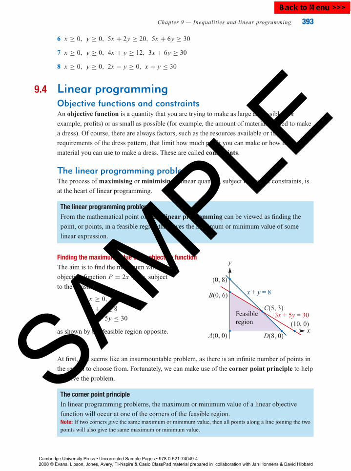
9.4 Linear programmingObjective functions and constraintsAn objective function is a quantity that you are trying to make as large as possible (for

example, profits) or as small as possible (for example, the amount of material needed to make

a dress). Of course, there are always factors, such as the resources available or the

requirements of the dress pattern, that limit how much profit you can make or how little

material you can use to make a dress. These are called constraints.

The linear programming problemThe process of maximising or minimising a linear quantity, subject to a set of constraints, is

at the heart of linear programming.

The linear programming problemFrom the mathematical point of view, linear programming can be viewed as finding the

point, or points, in a feasible region that gives the maximum or minimum value of some

linear expression.

Finding the maximum value of an objective functionThe aim is to find the maximum value of the

objective function P = 2x + 3y, subject

to the constraints:

x ≥ 0, y ≥ 0

x + y ≤ 8

3x + 5y ≤ 30

as shown by the feasible region opposite.

C(5, 3)

x

y

3x + 5y = 30

x + y = 8

(0, 8)

B(0, 6)

D(8, 0)

(10, 0)

Feasibleregion

A(0, 0)

At first, this seems like an insurmountable problem, as there is an infinite number of points in

the region to choose from. Fortunately, we can make use of the corner point principle to help

us solve the problem.

The corner point principleIn linear programming problems, the maximum or minimum value of a linear objective

function will occur at one of the corners of the feasible region.Note: If two corners give the same maximum or minimum value, then all points along a line joining the twopoints will also give the same maximum or minimum value.


SAMPLE

Back to Menu >>>



This means that we only need to evaluate

the objective function at each of the corner

points, labelled A, B, C and D, and find

which gives the maximum value. It helps to

set up a table as follows.

Objective function

Points P = 2x + 3y

A (0, 0) P = 2 × 0 + 3 × 0 = 0

B (0, 6) P = 2 × 0 + 3 × 6 = 18

C (5, 3) P = 2 × 5 + 3 × 3 = 19

D (8, 0) P = 2 × 8 + 3 × 0 = 16

Thus, the maximum value of the objective function, P = 19, occurs when x = 5 and y = 3.

Example 8 Finding the minimum value of an objective function

Find the minimum value of the objective

function C = 5x + 2y, subject to the

constraints:

x ≥ 0, y ≥ 0

x + 2y ≥ 10

6x + 4y ≥ 36

as displayed in the feasible region opposite.

A

B

C

(0, 9)

(0, 6)

x + 2y = 10

x

y

(0, 5)

(10, 0)O6x + 4y = 36

(4, 3)

Feasibleregion

Solution

1 Set up a table for the objective

function.

2 Evaluate the objective function at

each of the corners A, B and C.

3 Identify the corner point giving the

minimum value and write your answer.The minimum value is C = 18, which

occurs when x = 0 and y = 9.

Objective function

Points C = 5x + 2y

A(0, 9) C = 5 × 0 + 2 × 9 = 18

B(4, 3) C = 5 × 4 + 2 × 3 = 26

C(10, 0) C = 5 × 10 + 2 × 0 = 50

Exercise 9D

For each of the following objective functions and feasible regions, find the maximum or

minimum value (as required) and the point at which it occurs.

1 P = 4x + 2y (maximum) 2 P = 3x + 4y (maximum)

x

y

D(6, 0)

C(3, 3)B(0, 5)

A(0, 0)

Feasibleregion

x

y

D(6, 8)

C(2, 12)B(0, 10)

A(0, 0)

Feasibleregion

E(12, 0)


SAMPLE

Back to Menu >>>



3 C = 3x + 5y (minimum)

x

y

Feasibleregion

O

C(6, 0)

B(3, 2.5)

A(0, 10)

4 C = x + y (minimum)

x

y

Feasibleregion

O

C(10, 0)B(2, 4)

A(0, 12)

5 P = x + 2y (maximum)

x

y

C(30, 0)

B(10, 20)

A(0, 0)

Feasibleregion

6 C = 2x + 2y (minimum)

x

y

B(5, 0)

A(0, 5)

Feasibleregion

O

9.5 Linear programming applicationsYou now have all the technical skills necessary to set up and solve a basic linear programming

problem.

Example 9 Setting up and solving a maximising problem

A manufacturer makes two sorts of orange-flavoured chocolates: House Brand and Orange

Delights.

1 kg of House Brand contains 0.3 kg of chocolate and 0.7 kg of orange fill.

1 kg of Orange Delights contains 0.5 kg of chocolate and 0.5 kg of orange fill.

300 kg of chocolate and 350 kg of orange fill are available to the manufacturer each day.

The profit is $7.50 per kilogram on House Brand and $10 per kilogram on Orange

Delights.

How much of each type of

orange-flavoured chocolate should be

made each day to maximise profit?


SAMPLE

Back to Menu >>>



Solution

1 Define x and y. Let x be the amount (in kg) of House Brand

made each day.

Let y be the amount (in kg) of Orange

Delights made each day.

2 Write down the constraints.� x and y cannot be negative.� 300 kg of chocolate is available.� 350 kg of orange fill is available.

Constraints:

x ≥ 0, y ≥ 0

0.3x + 0.5y ≤ 300 (chocolate)

0.7x + 0.5y ≤ 350 (orange fill)

3 Graph the feasible region defined by

the constraints. Mark in each of the

corner points and label with their

coordinates. Use a calculator to

determine the point of intersection.

x

y

A(0, 0)

(0, 700)

B(0, 600)

C (125, 525)

D(500, 0) (1000, 0)

Feasible

region

0.3x + 0.5y = 300

0.7x + 0.5y = 350

4 Write down the objective function

(in dollars). Call it P, for profit.

Objective function:

P = 7.5x + 10y

5 Determine the maximum profit by

evaluating the objective function at

each corner of the feasible region.

Objective function

Point P = 7.5x + 10y

A(0, 0) P = 7.5 × 0 + 10 × 0 = $0

B(0, 600) P = 7.5 × 0 + 10 × 600

= $6000

C(125, 525) P = 7.5 × 125 + 10 × 525

= $6187.50

D(500, 0) P = 7.5 × 500 + 10 × 0

= $3750

6 Write your answer to the question. The maximum profit is $6187.50, which is

obtained by making 125 kg of House Brand

and 525 kg of Orange Delights.


SAMPLE

Back to Menu >>>



Example 10 Setting up and solving a minimising problem

SpeedGro and Powerfeed are two popular brands of home garden fertiliser. They both contain

the nutrients X, Y and Z, needed for healthy plant growth.

1 kg of SpeedGro contains 30 units of X, 50 units of Y and 10 units of Z.

1 kg of Powerfeed contains 20 units of X, 20 units of Y and 20 units of Z.

A gardener calculates that he needs a fertiliser containing at least 160 units of nutrient X,

200 units of nutrient Y and 80 units of nutrient Z.

Speedgro costs $8 per kg and Powerfeed costs $6 per kg.

How much of each type of fertiliser should he buy to meet his needs at the minimum cost?

Solution

1 Define x and y. Let x be the amount (in kg) of

SpeedGro needed.

Let y be the amount (in kg) of

Powerfeed needed.

2 Write down the constraints.� x and y cannot be negative.� At least 160 units of X are needed.� At least 200 units of Y are needed.� At least 80 units of Z are needed.

Constraints:

x ≥ 0, y ≥ 0

30x + 20y ≥ 160 (nutrient X)

50x + 20y ≥ 200 (nutrient Y)

10x + 20y ≥ 80 (nutrient Z)

3 Graph the feasible region defined by the

constraints. Mark in each of the corner

points and label with their coordinates.

Use a calculator to determine the points

of intersection. B(2, 5)

A(0, 10)

C (4, 2)

(0, 8)

(0, 4)

(4, 0)

D(8, 0)

(5.3, 0)50x + 20y = 200

30x + 20y = 16010x + 20y = 80

Feasible

region

x

y

O

4 Write down the objective function

(in dollars). Call it C, for cost.

Objective function:

C = 8x + 6y

5 Determine the minimum cost by

evaluating the objective function at

each corner of the feasible region.

Objective function

Point C = 8x + 6y

A(0, 10) C = 8 × 0 + 6 × 10 = $60

B(2, 5) C = 8 × 2 + 6 × 5 = $46

C(4, 2) C = 8 × 4 + 6 × 2 = $44

D(8, 0) C = 8 × 8 + 6 × 0 = $64

6 Write your answer to the question. The minimum cost is $44, which is

achieved by buying 4 kg of

SpeedGro and 2 kg of Powerfeed.


SAMPLE

Back to Menu >>>



Exercise 9E

1 A factory makes two products: Wigits and Gigits. Two different machines are used.� To make a Wigit takes 1 hour on Machine 1 and 2 hours on Machine 2.� To make a Gigit takes 1 hour on Machine 1 and 4 hours on Machine 2.� Up to 8 hours of Machine 1 time and up to 24 hours of Machine 2 time are available each

day.� The factory makes a profit of $200 for each Wigit and $360 for each Gigit it produces.

a Let x be the number of Wigits made each day.

Let y be the number of Gigits made each day.

The constraints for this problem are:

x ≥ 0, y ≥x + y ≤ 8 (Machine 1 time)

x + 4y ≤ (Machine 2 time)

Determine the missing information.

b The feasible region is shown on the right. Some

information is missing. Determine the missing

information.

x

y

A(0, 0)

Feasibleregion

D(8, 0)

(0, 8)x + y = 8

= 24

B

C

( )

c The objective function is give by P = 200x + y, where P stands for profit (in dollars).


d How many Wigits and Gigits should be made each day to maximise profit, and what is

this profit?

2 An outdoor clothing manufacturer makes two sorts of jackets: Polarbear and Polarfox.� To make a Polarbear jacket takes 2 m of material. The time taken to make a Polarbear

jacket is 2.4 hours.� To make a Polarfox jacket takes 2 m of material. The time taken to make a Polarfox

jacket is 3.2 hours.� The manufacturer has 520 m of material available and 672 hours of worker time to

make the jackets.� The manufacturer makes a profit of $36 for each Polarbear jacket and $42 for each

Polarfox jacket it produces.


SAMPLE

Back to Menu >>>



a Let x be the number of Polarbear jackets made.

Let y be the number of Polarfox jackets made.


x ≥ , y ≥x + 2y ≤ (material availability)

x + y ≤ 672 (worker time availability)




information.

x

y

A(0, 0)

Feasibleregion

= 520

= 672

D ( )

C ( )

E ( )

B(0, 210)

c The objective function is given by P = x + y, where P stands for profit (in dollars)


d What is the maximum profit that can be made, and how many Polarbear jackets and

Polarfox jackets should be made each day to achieve this profit?

3 Following a natural disaster, the army plans to use helicopters to transport medical teams

and their equipment into a remote area. They have two types of helicopter: Redhawks and

Blackjets.� Redhawks carry 45 people and 3 tonnes of equipment.� Blackjets carry 30 people and 4 tonnes of equipment.� At least 450 people and 36 tonnes of equipment need to be transported.� Redhawks cost $3600 per hour to run and Blackjets cost $3200 per hour to run.

a Let x be the number of Redhawks.

Let y be the number of Blackjets.


x ≥ 0, y ≥ 0

(people)

(equipment)



SAMPLE

Back to Menu >>>





information.

x

y

A(0, 15)Feasibleregion

C(12, 0)

( )

( )

B( )

= 450 = 36O

c The objective function is given by C = x + y, where C stands for cost (in

dollars). Determine the missing information.

d How many Redhawks and Blackjets should be used to minimise the cost per hour, and

what is this cost?

4 A sawmill produces both construction grade and furniture grade timber.� To produce 1 cubic metre of construction grade timber takes 2 hours of sawing and

3 hours of planing.� To produce 1 cubic metre of furniture grade timber takes 2 hours of sawing and 6 hours of

planing.� Up to 8 hours of sawing time and 18 hours of planing time are available each day.� The sawmill makes a profit of $500 per cubic metre of construction grade timber and

$600 per cubic metre of furniture grade timber it produces.

a Write down the constraints and profit function for this problem.

b Draw a diagram.

c Find how much construction grade and furniture grade timber the sawmill should make

each day to maximise its profit. What is this profit?

5 Two breakfast cereal mixes, Healthystart and Wakeup, are available in bulk.� Each kilogram of Healthystart contains 12 mg of vitamin B1 and 40 mg of vitamin B2.� Each kilogram of Wakeup contains 20 mg of vitamin B1 and 25 mg of vitamin B2.� You want a mix of the two that contains at least 15 mg of vitamin B1 and 30 mg of

vitamin B2.� Healthystart costs $5 a kilogram and Wakeup costs $4.50 per kilogram.

a Write down the constraints and cost function for this problem.

b Draw a diagram.

c Find the mixture of these two cereals that will meet your needs at minimum cost. What is

this cost?


SAMPLE

Back to Menu >>>


Review


Key ideas and chapter summary

Linear inequality A linear inequality involves one or two of the signs >, ≥, < or ≤,

but not an equals sign ( = ).

Displaying linear A linear inequality in one variable can be represented on a number

line by a solid coloured line ending at one or two circles.

The line represents all the possible solutions of the inequality.

An open circle (◦) indicates that the end value is not included in the

inequality (for < or >).

A closed circle (•) indicates that the end value is included in the

inequality (for ≤ or ≥).

inequalities in one

variable on a number

line

Displaying linear Linear inequalities in one variable can be represented on a

coordinate plane by a shaded region bounded by one or two lines

parallel to the x- or y-axes.

The region represents all the possible solutions of the inequality.

A dashed line indicates that the line is not included in the inequality

(for < or >).

A solid line indicates that the line is included in the inequality

(for ≤ or ≥).

inequalities in one

variable on the

coordinate plane

Displaying linear A linear inequality in two variables can be represented on a

coordinate plane by a shaded region bounded by a line at an angle to

the x- and y-axes.

The region represents all the possible solutions of the inequality.

The boundary line is dashed if it is not included in the inequality

(for < or >), but solid if it is included (for ≤ or ≥).

A reference point, often the origin (0, 0), can be used to help decide

whether the required region lies above or below the line.

inequalities in two

variables on the

coordinate plane

Feasible region When solving simultaneous inequalities, the region in the coordinate

plane that is common to all the inequalities is called the feasible

region. It represents all the possible solutions to the simultaneous

inequalities.

The feasible region can be found graphically (for a small number of

inequalities) by shading in the required regions for all the

inequalities and determining where they all overlap.

A graphics calculator can be used to graph a feasible region.

Linear programming Linear programming involves maximising or minimising a linear

quantity subject to the constraints represented by a set of linear

inequalities. The constraints (e.g. requirements, resources) define the

feasible region in which the quantity is to be maximised or

minimised.


SAMPLE

Back to Menu >>>


Rev

iew


The constraints x ≥ 0 and y ≥ 0 together restrict the feasible region

to the positive (first) quadrant.

Objective function The objective function is a linear expression representing the

quantity to be maximised (e.g. profit) or minimised (e.g. cost) in a

linear programming problem.

Corner point principle The corner point principle states that, in linear programming

problems, the maximum or minimum value of a linear objective

function will occur at one of the corners of the feasible region, or on

a line on the boundary of the feasible region joining two of the

corners.

Skills check

Having completed this topic you should be able to:

represent a linear inequality in one variable on a number line

represent a linear inequality in one or two variables on the coordinate plane

know the meaning of the terms feasible region, constraint and objective function as

they relate to linear programming

determine the maximum or minimum value of an objective function for a given

feasible region

set up and solve basic linear programming problems.

Multiple-choice questions

1 The inequality displayed on the number line on

the right is:–1 0 1 3 4 5 6 7 82

x

A 1 ≤ x ≤ 7 B 1 < x < 7 C 1 ≤ x < 7

D 1 < x ≤ 7 E 1 > x > 7

2 The inequality displayed on the number line on

the right is:–1 0 1 3 4 5 6 7 82

x

A x < 5 B x ≤ 5 C x > 5

D x ≥ 5 E 0 > x > 5

3 The inequality displayed on the coordinate plane

on the right is:

x

(0, 8) y = 8

O

y

A x < 8 B x ≤ 8 C y < 8

D y ≤ 8 E 0 > x > 8


SAMPLE

Back to Menu >>>


Review


4 The inequality displayed on the coordinate plane

on the right is:

Ox

x =

3

x =

10

y

(3, 0) (10, 0)

A 3 < x < 10 B 3 < x ≤ 10 C 3 ≤ x ≤ 10

D 3 < y < 10 E 3 < y ≤ 10

5 The equation of the line displayed on the right is:

O

(0, 4)

(5, 0)x

y

A 4x + 5y = 4 B 4x − 5y = 4 C 5x + 4y = 20

D 4x + 5y = 20 E 4x − 5y = 20

6 The equation of the line displayed on the right is:

(0, 0)

(5, 4)

x

y

A 4x − 5y = 0 B 4x + 5y = 0 C 5x − 4y = 20

D 5x + 4y = 20 E 5y = 20x

7 The region displayed on the right (including the line)

represents the inequality:

(4, 0)x

y

O

(0, 10)

5x + 2y = 20A 5x + 2y < 20 B 5x + 2y ≤ 20 C 5x + 2y > 20

D 5x + 2y ≥ 20 E 2x + 5y > 20

8 The region displayed on the right (not including the line)

represents the inequality:

(–2, 0)

(0, 6)

x

y

O

y – 3x = 6A y − 3x ≤ 6 B y − 3x < 6 C y − 3x ≥ 6

D y − 3x > 6 E 3x − y > 6


SAMPLE

Back to Menu >>>


Rev

iew


9 The two lines shown on the right intersect at the point:

x

y

3x + 4y = 12

x + 3y = 6

O

(0, 3)

(0, 2)

(4, 0) (6, 0)

A (1, 1.3) B (2, 1.5) C (1.2, 1.2)

D (2.4, 1.2) E (3, 2.4)

10 The feasible region displayed on the right

(including the line) is defined by the inequalities: (0, 5)

(5, 0)x

y

Feasibleregion

O

A x ≥ 0, y ≥ 0, x − y < 5

B x ≥ 0, y ≥ 0, x − y ≥ 5

C x ≥ 0, y ≥ 0, x + y < 5

D x ≥ 0, y ≥ 0, x + y ≤ 5

E x ≥ 0, y ≥ 0, x + y ≥ 5

11 The feasible region displayed on the right

(including the lines) is defined by the inequalities:

x + 2y = 104x + y = 12

(0, 12)

(0, 5) (2, 4)

(3, 0)

(10, 0)

Feasibleregion

x

y

O

A x ≥ 0, y ≥ 0, x + 2y ≥ 10, 4x + y ≥ 12

B x ≥ 0, y ≥ 0, x + 2y ≤ 10, 4x + y ≤ 12

C x ≥ 0, y ≥ 0, x + 2y > 10, 4x + y > 12

D x ≥ 0, y ≥ 0, x + 2y < 10, 4x + y < 12

E x ≥ 0, y ≥ 0, x + 2y ≥ 10, 4x + y ≤ 12

12 For the feasible region displayed in Question 11, the minimum value of the

objective function, C = 2x + y, is:

A 5 B 6 C 8 D 12 E 20

13 For the feasible region displayed on the right, the maximum

value of the objective function, P = 4x + 3y, is:(0, 12)

(0, 10)

(6, 6)

(0, 0) (12, 0)

Feasibleregion

x

y

(15, 0)

A 0 B 40 C 42

D 48 E 60

The following information relates to Questions 14 to 16An outdoor clothing manufacturer makes two styles of all-weather coats: long and short.� To make a short coat, 2 m of material are required. The time taken to make a short

coat is 2.5 hours.� To make a long coat, 3 m of material are required. The time taken to make a long

coat is 3.5 hours.


SAMPLE

Back to Menu >>>


Review


� The manufacturer has 450 m of material available and 700 hours of worker time to

make the coats.� The manufacturer makes a profit of $40 for each short coat and $48 for each long

coat.

Let x be the number of short coats made.

Let y be the number of long coats made.

14 The constraints that relate to the amount of material available are:

A x ≥ 0, y ≥ 0, 2x + 3y ≤ 450 B x ≥ 0, y ≥ 0, 2x + 3y ≥ 450

C x ≥ 0, y ≥ 0, 2.5x + 3.5y ≤ 700 D x ≥ 0, y ≥ 0, 2.5x + 3.5y ≥ 700

E x ≥ 0, y ≥ 0, 40x + 48y ≥ 700

15 The constraints that relate to the amount of time available are:

A x ≥ 0, y ≥ 0, 2x + 3y ≤ 450 B x ≥ 0, y ≥ 0, 2x + 3y ≥ 450

C x ≥ 0, y ≥ 0, 2.5x + 3.5y ≤ 700 D x ≥ 0, y ≥ 0, 2.5x + 3.5y ≥ 700

E x ≥ 0, y ≥ 0, 40x + 48y ≥ 700

16 The objective function P is:

A P = 2.5x + 3.5y B P = 2x + 3y C P = 3x + 3.5y

D P = 40x + 48y E P = 450x + 700y

Short-answer questions

1 Plot the inequality −2 ≤ x < 4 on a number line.

2 Plot the inequality 1 ≤ y < 5 on the coordinate plane.

3 Plot the inequality 5x + 4y < 40 on the coordinate plane.

4 Plot the region defined by the inequalities:

x ≥ 0, y ≥ 0, 3x + 5y ≤ 60

5 Plot the region defined by the inequalities:

x ≥ 0, y ≥ 0, 2x + 3y ≥ 30, x + 4y ≥ 20

Extended-response questions

1 A garden products company makes two sorts of fertiliser: Standard Grade and

Premium Grade. There are two main ingredients: nitrate and phosphate.� To make a tonne of Standard Grade fertiliser takes 0.8 tonnes of nitrate and 0.2

tonnes of phosphate.� To make a tonne of Premium Grade fertiliser takes 0.7 tonnes of nitrate and 0.3

tonnes of phosphate.� The company has 56 tonnes of nitrate and 21 tonnes of phosphate.� The company makes a profit of $600 per tonne on Standard Grade fertiliser and

$750 per tonne on Premium Grade fertiliser.


SAMPLE

Back to Menu >>>


Rev

iew


a Write the constraints and profit function for this problem.

b Draw a diagram.

c Find how much of each type of fertiliser the company should make to maximise

its profit. What will this profit be?

2 Two foods fed to animals contain both vitamin A and vitamin B.� 1 kg of Food A contains 3 units of vitamin A and 4 units of vitamin B.� 1 kg of Food B contains 5 units of vitamin A and 3 units of vitamin B.� The daily vitamin requirement of each animal is at least 15 units of vitamin A

and at least 12 units of vitamin B.� Food A costs $0.30 per kg and Food B costs $0.24 per kg.

a Write the constraints and cost function for this problem.

b Draw a diagram.

c Find how much of each type of food should be fed to the animals each day to

minimise cost. What is this cost?


SAMPLE

Back to Menu >>>

Inequalities and linear · PDF fileCHAPTER9 Inequalities and linear programming What is a...

Documents

Transcript of Inequalities and linear · PDF fileCHAPTER9 Inequalities and linear programming What is a...