LINEAR PHASED ARRAY OF COAXIALLY- FED MONOPOLE …

AD-A238 959

RL-TR-91-124In-House ReportApril 1991

LINEAR PHASED ARRAY OF COAXIALLY-FED MONOPOLE ELEMENTS IN APARALLEL PLATE WAVEGUIDE

Boris Tomasic and Alexander Hessel

APPROVED FOR PUBLUC RELEASE, DSTR77UON UNLIMITED

DTICft FLEC-I E

SAUG 5 1981U

Rome LaboratoryAir Force Systems Command

Griffiss Air Force Base, NY 13441-5700

91-06811

This report has been reviewed by the RADC Public Affairs Office (PA) and

is releasable to the National Technical Information Service (NTIS). At NTIS

it will be releasable to the general public, including foreign nations.

RL-TR-91-124 has been reviewed and is approved for publication.

APPROVED:

JOHN K. SCHINDLERChief, Antennas & Comp DivisionDirectorate of Electromagnetics

APPROVED:

PAUL J. FAIRBANKS, Lt Colonel, USAF

Deputy Director of Electromagnetics

FOR THE COMMANDER:

JAMES W. HYDE IIIDirectorate of Plans & Programs

If your address has changed or if you wish to be removed from the RADC

mailing list, or if the addressee is no longer employed by your organization,

please notify RADC (EEAA) Hanscom AFB MA 01731-5000. This will assist us in

maintaining a current mailing list.

Do not return copies of this report unless contractual obligations or

notices on a specific document require that it be returned.

REPORT DOCUMENTATION PAGE Form, Approved

OMB No. 0704-0188

Pubc reporing for io collection of Informaton Is eostnated to average I hour per respone. bIckludig tho ftr for re*,ewfng Inetruclons, searching existig date sources,ga ering and mernt*Vrn to, data needed. end conploeng e revwl te collection of Infor tion. Send coonto regarding ol burden osnmate or ano0w aspect of thecolectio of IrorniatIon. Including uggeefone fow reducing io buden, to Washington Heedquerter Services, Directorate for Information Operation. and Reports, 1215 JeffereonDaste Htgiay. Suite 1204. rlngton. VA 22202-4302, end to tie Dice of Management and Budget Peperwlm Reduction Project (0704-01 S). Wauhngton, DC 20503.

1. AGENCY USE ONLY (Leave blez*) 2. REPORT DATE I3.REPORIT TYPE AND DATES COVERED

April 1991 ln-House 1 Jan 83 to 31 Dec 86

4. TITLE AND SUBTITLE S. FUNDING NUMBERS

Linear Phased Array of Coaxially-Fed Monopole Elements in a PE 61102FParallel Plate Waveguide PR 2305

TA J3G. AUTHOR(S) WU 03

Boris Tomasic and Alexander Hessel*

7. PERFORMING ORGANIZATION NAME(S) AND ADDRESS(ES) .PERFORMING ORGANIZATIONREPORT NUMBER

Rome Laboratory RL-TR-91-124RL/EEAAHanscom AFBMassachusetts 01731-5000

9. SPONSORINQ/4ONITORING AGENCY NAME(S) AND ADDRESS(ES) 10. SPONSORING/MONITORINGAGENCY REPORT NUMBER

11. SUPPLEMENTARY NOTES'Weber Research Institude, Polytechnic University, Farmingdale. NY 11735

12a. DISTRIBUTIONAVAILABILITY STATEMENT 12b. DISTRIBUTION COOE

Approved for public release; distribution unlimited

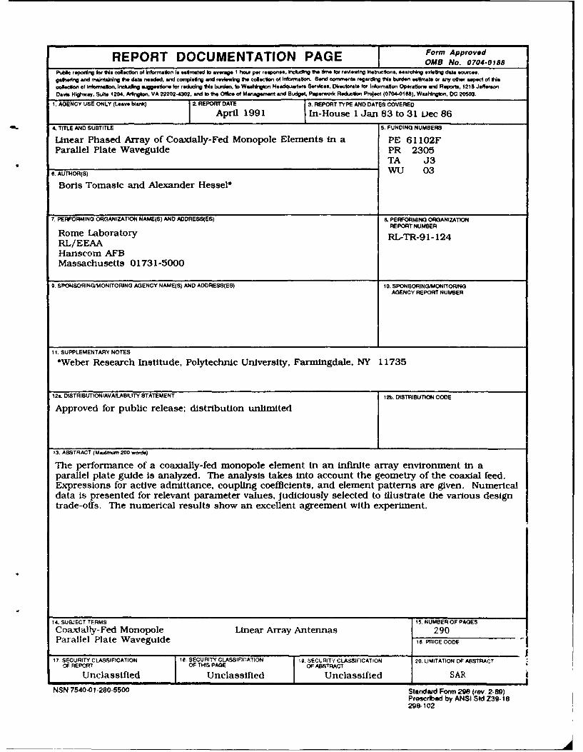
13. ABSTRACT )Mantmu.ni 200 worde)

The performance of a coaxially-fed monopole element in an infinite array environment in aparallel plate guide is analyzed. The analysis takes into account the geometry of the coaxial feed.Expressions for active admittance, coupling coefficients, and element patterns are given. Numericaldata is presented for relevant parameter values. judiciously selected to illustrate the various designtrade-offs. The numerical results show an excellent agreement with experiment.

14. SUB.JECT TERMS IS. NUMBER OF PAGESCoaxially-Fed Monopole Linear Array Antennas 290Parallel Plate Waveguide I. PRICE CODE

117. SECURITY CLASSIFICATION |I e. SECURITY CLASSIFICATION 9. SECURITY CLASSIFICATION 20. LIMITATION OF ABSTRACT

OF REPOtr OF THIS PAGE OF ABSTRACT

Unclassified Unclassified Unclassified SAR

NSN 7540-01-280-5500 Standard Form 299 (rev 2-99)Prescrbed by ANSI Std Z39-1 8298-102

Looessloml ow .

NTIS GRA&I R06DTIC TAB 0

Unannounced QJustiftcatio

ByDistribution/

Availability Codes

Avail and/or

Dist Special

Contents

1. INTRODUCTION 1

2. MAGNETIC RING SOURCE IN AN INFINITE PARALLEL PLATE WAVEGUIDE 3

2.1 Green's Functions 52.2 Hertz Potential 112.3 Vector Potential 132.4 Electric Field (EP, Ez) 172.5 Magnetic Field (H,) 20

3. CYLINDRICAL ELECTRIC CURRENT SOURCE IN AN INFINITE PARALLEL PLATE 21WAVEGUIDE

3.1 Green's Functions 22

3.2 Hertz Potential 23

3.3 Vector Potential 253.4 Electric Field (Ep, Ez) 253.5 Magnetic Field (H ) 26

4. ACTIVE ADMITTANCE AND REFLECTION COEFFICIENT OF AN INFINITE LINEAR 27PHASED ARRAY OF MONOPOLE ELEMENTS IN A PARALLEL PLATE WAVEGUIDE

4.1 Coaxially-Fed Monopole in an Infinite Parallel Plate Waveguide 294.1.1 Vector Potential Ao(p,z) 304.1.2 Electric Field Eo(P,z)

4.1.3 Magnetic Field Ho(P,z) 33

4.2 Total Axial Electric. k,(a,z) on the [robe Surfacc '3_I

iit

.43 e b &dft,. J.(z) 41

4.4' Total Magnetic Feld in the Aperture H. (a S p _<b, z-O+) 44

4.5 Active Admittance, Y.(8x) 49

4.6 Active Reflection Coefficient, a(8 ) 57

4.7 Coupling (Scattering) Coefficients, SP 58

5. FAR FIELD PATTERN OF THE SINGLE MONOPOLE IN AN INFINITE AND SEMI- 60INFINITE PARALLEL PLATE REGION

5.1 Far Fleld Ezo(p,t) Represented in Terms of Radial Modes 60

5.2 Single Monopole Gain Pattern g e) 65

6. FAR-FIELD ELEMENT PATTERN OF AN INFINITE ARRAY RADIATING INTO AN 68

INFINITE AND A SEMI-INFINITE PARALLEL PLATE REGION

6.1 Far-Field of the Active Array Ez(p,*) Represented in Terms of Radial Modes 69

6.2 Far-Field of the Active Array Ez(xy) Represented in Terms of Floquet Modes 71in a Unit Cell

6.3 Element Pattern ge)(e) 76

7. NUMERICAL ANALYSIS 85

8. NUMERICAL RESULTS AND DISCUSSION 91

8.1 Single Monopole in an Infinite Parallel Plate Region 91

8.2 Single Monopole in a Semi-Infinite Parallel Plate Region 1078.3 Linear Array of Coaxally-fed Monopole Elements in an 127

Infinite Parallel Plate Waveguide8.3.1 Active Admittance, Ya(81) 1278.3.2 Probe Current, IZ(Z) 135

8.3.3 Coupling Coefficients, S P 1438.4 Linear Array of Coalally-fed Monopole Elements in a Semi-Infinite Parallel 147

Plate Waveguide8.4.1 Active Admittance, Y.(8.) 1478.4.2 Probe Current, Iz(z) 158

8.4.3 Coupling Coefficients, SP 166

8.4.4 Element Pattern, g (e)(.) 169

9. EXPERIMENTS 174

9.1 Array Description 1759.2 Monopole Element Design 1789.3 Waveguide Simulator 1789.4 Coupling Coefficients 1839.5 Element Pattern 185

iv

10. CONCLUSIONS 189

REFERENCES 191

APPENDIX A Field Representation in Regions with Piecewise Constant Properties 193

Al Derivation of the Time-Harmonic Field from Scalar Potentials 19Z

A2 Modal Representation for Unbounded Cross Sections 197

APPENDIX B Magnetic Ring Source in an Infinite Parallel Plate Waveguide - Radial 203

Mode Representation

BI Radial Transmission Line Representation 203

B2 Radial Magnetic Green's Function Representation 212

APPENDIX C Cylindrical Electric Current Source in an Infinite Parallel Plate 221

Waveguide - Radial Mode RepresentationCl Radial Transmission Line Representation 221

C2 Radial Electric Green's Function Representation 225

APPENDIX D Addition Theorem for Hankel Functions 233

APPENDIX E Convergence Acceleration of Series Sn(b,) 235El Infinite Linear Array of Monopole Elements in an Infinite 235

Parallel Plate WaveguideE2 Infinite Linear Array of Monopole Elements in a Semi-Infinite 238

Parallel Plate Waveguide

APPENDIX F The Fourier Integral of the Hankel Function 241

APPENDIX G The Stationary-Phase Method for Evaluation of Integrals 245

APPENDIX H Test for Power Conservation 247HI Evaluation of the Complex Poynting Vector Over the Coaxial 251

Aperture Area

H2 Evaluation of the Complex Poynting Vector Over the Probe Surface 256

H3 Evaluation of the Complex Poynting Vector Over the Unit Cell 260

Cross-Section Area

APPENDIX I Numerical Evaluation of the Integral I (Q) f(x) e-lxdx 26)

v

Illustrations

2-1. Geometry of Coaxially Driven Annular Aperture In an Infinite Parallel Plate 4Waveguide

2-2. Magnetic Ring Source in an Infinite Parallel Plate Wavegulde 4

2-3. Magnetic Point Source in an InEinite Parallel Plate Waveguide 6

2-4. Network Problem for the Determination of Y (Z. Z') 7

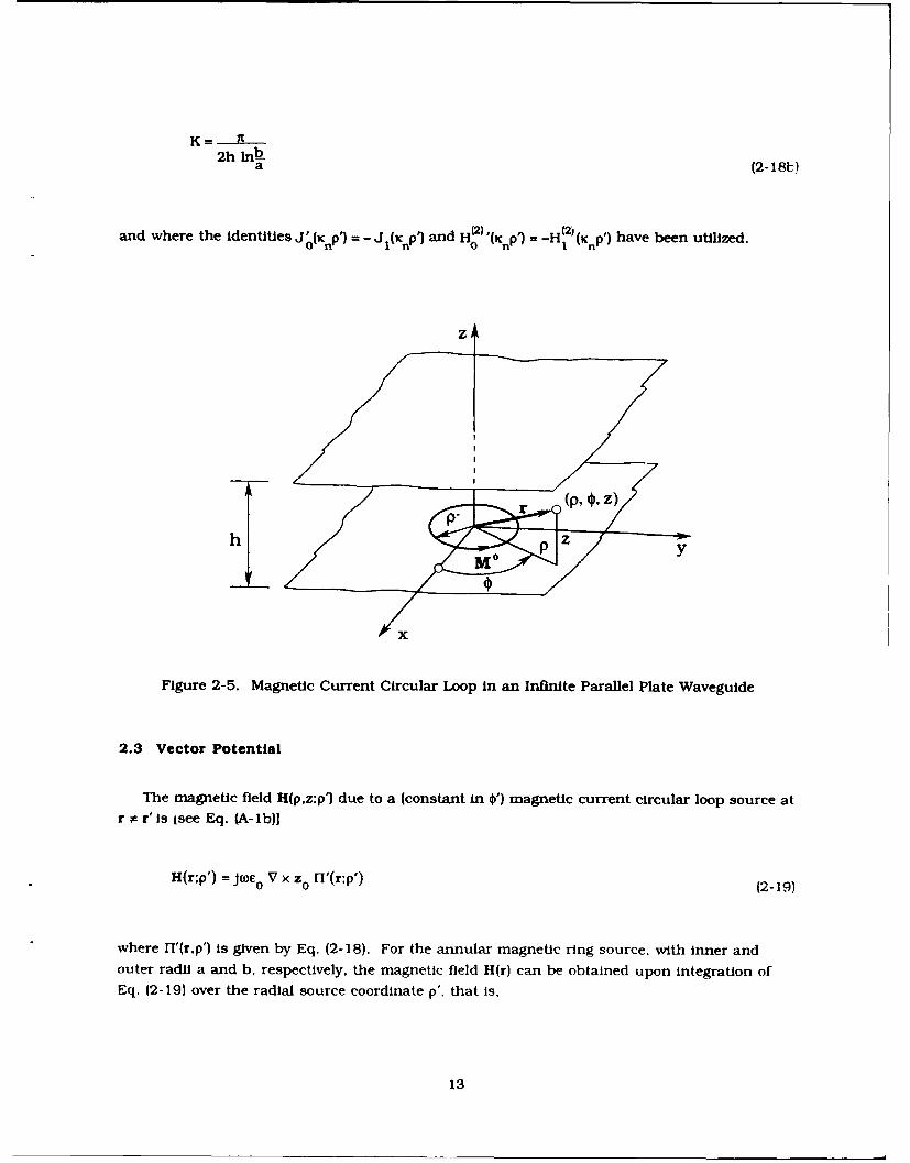
2-5. Magnetic Current Circular Loop, in an Inftn.te Parallel Plate Wavegulde 13

3-1. Geometry of Cylindrical Electric Current Source in an Infinite Parallel Plate 22Waveguide

3-2. Axial Electric Dipole in an Infinite Parallel Plate Wavegulde 23

4-1. Linear Array of Coaxlal-Monopole Elements in a Semni-Infinite Parallel Plate 27Wavegulde

4-2. Coa~dally-Fed Monopole In an Infinite Parallel Plate Wavegulde 294-3. Geometry of the Linear Array and Its Image for Evaluation of E2(a.z) (Top View) 35

4-4. Trangle Pertaining to the Addition Theorem for Hankel Functions 37

4-5. Geometry of Linear Array and Its Image for Evaluation of A_(a < p 5<b. z = 0+) 45

(Top View)

vi

4-6. Triangle Pertaining to Addition Theorem for Hankel Functions 48

4-7. Active Infinite Linear Array Pertaining to Uniform-Amplitude, Linear-Phase 49

Progression Excitation

4-8. Infinite Linear Array Pertaining to the Definition of Coupling (Scattering) 59

Coefficients

5-1. Coaxially-fed Monopole and Its Image in an Infinite Parallel Plate Region 62

6-1. Infinite Linear Array Pertaining to Single Element Excitation 69

6-2. Geometry of the Linear Array and its Image for Evaluation of Ez(p. ) (Top View) 71

(U=1 case shown)

6-3. Unit Cell Geometry of an Infinite Linear Array of Coaxially-fed Monopoles in a 71

Semi-Infinite Parallel Plate Waveguide

7-1. Active Conductance vs Number of Probe Current Terms (d/k = 0.4, h/4 = 0.369, 87

s/X = 0.163. a/?, = 0.006, b/K = 0.034, Zc. = 50 ; ;o = 00)

7-2. Active Susceptance vs Number of Probe Current Terms (d/, = 0.4, h/K f 0.369, 88

q/. = 0.163, a/K = 0.0106, b/K = 0.034, Z¢ = 50 f; = 0 ° )

8-1. Input Conductance vs Probe Length; Parameter: Parellel Plate Separation 92

h/X= 0.3, 0.35. 0.4 (a/, = 0.016, b/?, = 0.037)

8-2. Input Susceptance vs Probe Length; Parameter: Parallel Plate Separation 93

h/K= 0.3, 0.35, 0.4 (a/;. = 0.016, b/% = 0.037)

8-3. Input Admittance vs Probe Length, (h/?. = 0.95, a/?, = 0.016, b/K = 0.037) 94

8-4. Reflection Coefficient (Contour Plot of Magnitude) vs Parallel Plate Separation 95

and Probe Length, (a/, = 0.016, b/K, = 0.037)

8-5. Input Impendence vs Probe Length, (h/?, = 0.35, a/K = 0.016, b/. = 0.037, ZN = 50 Ql) 96

8-6. Input Impedance vs Frequency, (h /XC = 0.35, Ic/?., = 0.24, a/?,, = 0.016. b/k c = 0.037 97

ZN = 50 )

8-7. Input Admittance vs Probe Radius, (h,,/K = 0.35, Ic/K = 0.24, b/K = 2.3 a/K 98

Ze = 50 Q)

8-8. Current Distribution (Amplitude) Along a Coaxially-Driven Monopole in an 99Infinite Parallel Plate Region; Parameter: Probe Length 1/K, = 0.1. 0.2. 0.3,

(h/K = 0.4. a/k = 0.016, b/K = 0.037)

.-9. Current Distribution (Phase) Along a Coaxially-Driven Monopole in an 100

Infinite Parallel Plate Region: Parameter: Probe LenIwtlh 1/, = 0.1. 0.2. 0.3,

(h/Ki = 0.4. a/k = 0.016. b/k = 0.037)

8-10. Current Distribution (Aiplitude) Along a Coaxially-Diiven Monopole in an 10'I

Infinite Parallel Plate Waveguide; Parameter: Total Ntimber of Current Terms I = 1,10, (lc/K = 0.24. h,/K = 0.35, a/K = 0.016, b/K = 0.037)

vii

8-11. Current Distribution (Phase) Along a Coaxially-Driven Monopole in an 104

Infinite Parallel Plate Waveguide, Parameter: Total Number of Current Terms I = 1,10, (1,/)X = 0.24, hJX = 0.35, a/X = 0.016, b/X = 0.037)

8-12. Current Distribution (Amplitude) Along a Coaidally-Driven Monopole in an 105

Infinite Parallel Plate Waveguide; Parameter: Total Number of Current Terms I = 1.

10, (l X = 0.75, h/X = 0.95, a/X = 0.016, b/X = 0.037)

8-13. Current Distribution (Phase) Along a Coaxially-Driven Monopole in an 106Infinite Parallel Plate Waveguide; Parameter: Total Number of Current Terms I = 1,

10, (I/X = 0.75, h/X = 0.95, a X = 0.016, b/X = 0.037)

8-14. Input Conductance vs Probe Length; Parameter: Parallel Plate Separation 108h/X = 0.3, 0.35, 0.4, (a X = 0.0 16, b/X = 0.037, s/X = 0.25)

8-15. Input Susceptance vs Probe Length; Parameter: Parallel Plate Separation 109

h/X = 0.3. 0.35, 0.4. (a X = 0.0 16, b/X = 0.037, s/X = 0.25)

8-16. Reflection Coefficient (Contour Plot of Magnitude) vs Probe-Ground Distance 110

and Probe Length (h/WX = 0.35, a/X = 0.016. b/X = 0.037)

8-17 Input Impedance vs Probe-Ground Distance and Probe Length. (h/X = 0.35. illa/X = 0.016, b X = 0.037, ZN = 50 Q)

8-18. Input Impedance vs Probe-Ground Distance, (1,,/X = 0.2187) and vs Probe Length 112

(sc/X = 0.2275), (h/X = .35, a/X = 0.016, b/X = 0.037, ZN = 50 ")

8-19. Input Impedance vs Frequency (h/X.c = 0.35, 1/Xc. = 0.2187, s,/Xe = 0.2275. 113a/X = 0.016, b/X c = 0.037, ZN = 50 Q)

8-20. Input Admittance vs Probe Radius (h/X = 0.35, se/X = 0.2275, Ic/X = 0.2187, 114

b/, = 2.3 aiX, ZN = 50 U)

8-21. Current Distribution Along a Coaxially-Driven Monopole in a Semi-Infinite 115

Parallel Plate Region, (h/X = 0.35, I/X = 0.15. s/X = 0.15. a X = 0.016, b/X = 0.037)


Parallel Plate Region. (h X = 0.35, I/X = 0.3, s X = 0.15. a X = 0.0 16. b/X = 0.037)


Parallel Plate Region, (h/X = 0.35. I/X = 0.15. s/X = 0.3. a X = 0.016, b/X = 0.037)


Parallel Plate Region, (h/X = 0.35, I/X = 0.3, s X = 0.3, a/X = 0.016. b/X = 0.037)

8-25. Current Distribution Along a Coaxially-Driven Monopole in a Semi-Infinite 119Parallel Plate Region, (h/X = 0.35, 1,/?, = 0.2187, s/X = 0.2275, a/X = 0.016.

b/. = 0.037)

8-26. Gain Pattern (h/WX = 0.35. lI/i = 0.15, a/X = 0.016. b/X = 0.037. Z = 50 Q2) 124

Parameter: s/. = 0.15, 0.3

8-27. Gain Pattern (h/WX = 0.35, I/X = 0.3, a/X = 0.016. b/X = 0.037. Z, = 50 fl). 125

Parameter: s/X = 0.15, 0.3

viii

8-28. Gain Pattern h/. = 0.35, Ic/, = 0.2187, s,/X = 0.2275, a/X = 0.016, b/X = 0.037, 126

z, = 50 a)

8-29. Active Reflection Coefficient (Contour Plot of Magnitude) vs Parallel Plate Height 128

and vs Probe Length (d/WX = 0.4, a/X = 0.016, b/X = 0.0343, Z, = 50 Q, Oo = 00)

8-30. Active Reflection Coefficient (Contour Plot of Magnitude) vs Parallel Plate Height 12 c

and vs Probe Length (d/WX = 0.6, a/X = 0.0106, b/X = 0.0343, Zc = 50 0. o = 00)

8-31. Active Impedence vs Parallel Plate Distance and vs Probe Length - Matched Case 130

(d/X = 0.4, hc/X = 0.36, lc/X = 0.28, a/X = 0.0106, b/X = 0.0343, Z: = 50 0, 0o = 0 -)

8-32. Active Impedence vs Parallel Plate Distance and vs Probe Length (d/X = 0.6, 131

h/2, = 0.36, I/. = 0.28, a/?L = 0.0106, b/X = 0.0343. Z = 50 fl, o = 0 )

8-33. Active Impedence vs Probe Radius (Array (a): d/X = 0.4, hc/X = 0.36, /X = 0.28, 132

b = 3.249 a, Z = 50 (1, 0o = 00; Array (b): d/7, = 0.6, h/% = 0.36. I/X = 0.28,

b = 3.249 a, ZC = 50 fl, o = 0 ° )

8-34. Active Impedence vs Frequency (Array (a): d/X c = 0.4, hc/l c = 0.36, Ic/X. = 0.28, 133

b/X c = 3.249 a/Xe, Zc = 50 Q, o = 00; Array (b): d/X c = 0.6, h/X c = 0.36, I/X c = 0.28..

b/. c = 3.249 a/X., ZC = 50 0, o = 0 ° )

8-35. Active Impedence vs Scan; Parameter: Frequency f = 0.9 f, fc' and 1. 1 fc 134

(d/Xc = 0.4, hc/?Lc = 0.36, Ic/. c = 0.28, a/Xe = 0.0106, b/ c = 0.0343, Z, = 50 11)

8-36. Active Impedence vs Scan; Parameter: Frequency f = 0.9 fc, fc' and 1. 1 fc 135

(d/ . = 0.6, h/X = 0.36, l/k = 0.28, a/X = 0.0106, a/Xc = 0.0343, Z = 50 )

8-37. Probe Current - Magnitude; Parameter: I/X = 0.15, 0.28, and 0.3 (d/X = 0.4, 136

h/X = 0.36, a/x = 0.0106, b/ = 0.0343, Zc = 50 2, o 0 °)

8-38. Probe Current - Phase: Parameter: Iix = 0.15, 0.28, and 0.3 (d/X = 0.4. 137

h/X = 0.36, a/ = 0.0106, b/X = 0.0343, ZC = 50 fl, o = 00)

8-39. Probe Current - Magnitude- Parameter: I/ti = 0.15, 0.28, and 0.3 (d/X = 0.6, 132

h/X = 0.36, a/k = 0.0106, b/X = 0.0343, Z, = 50 0, o = 00)

3-40. Probe Current - Phase; Parameter: l[I. = 0.15, 0.28, and 0.3 (d/X = 0.6, 139

h/X = 0.36, a/X = 0.0106, b/X = 0.0343. Z( = 50 f2, 0)

Ix

8-41. Amplitude of Coupling Coefficients vs Element Serial Number; Parameter: 144d[Z = 0.4, 0.6 [Array (a): d/X = 0.4, he/% = 0.36, 1c/X --0.28, a/X = 0.0106. b/X = 0.0343.Z, = 50 fQ: Array (b): d/X = 0.6, h/k = 0.36, I/X = 0.28. a/% = 0.0106, b[X = 0.0343.z c = 50 al

8-42. Phase of Coupling Coefficients vs Element Serial Number; Parameter: 146

d/X = 0.4, 0.6 [Array (a): d/X = 0.4, h/X = 0.36, I/X --0.28, a/X = 0.0106, b/X = 0.0343,Zc = 50 fQ; Array (b): d/X = 0.6, h/Z = 0.36, I/X = 0.28..a/X = 0.0106, b/k = 0.0343,z c = 50 fl]

8-43. Active Impedance vs Probe-Ground Distance s/X and vs Probe Length I/X 148

(d/X = 0.4, o = 0-)

8-44. Active Impedance vs Probe-Ground Distance s/X and vs Probe Length I/X 149

(d/X = 0.6, 'o = 0 9)

8-45. Active Reflection Coefficient - Maginitude vs Probe-Ground Distance s/X and vs 150

Probe Length 1iX (d/X = 0.4. %o = 00)

8-46. Active Reflection Coefficient - Maginitude vs Probe-Ground Distance s/X and vs 151

Probe Length l/X (d/X = 0.6. 4o = 0 )

8-47. Active Impedance vs Probe-Ground Distance s/x and vs Probe Length /X for 152

Array (a) - see Eq. (8-5) for Specifications, ( 0 = 0 )

8-48. Active Impedance vs Probe-Ground Distance s/x and vs Probe Length I/x for 153

Array (b) - see Eq. (8-5) for Specifications, (;o = 0 )

8-49. Active Impedance vs Parallel Plate Height h/X for Arrays (a) and (b), (o =0 ) 154

8-50. Active Impedance vs Probe Radius for Arrays (a) and (b). (b - 3.249 a. o =0 ) 155

8-51. Active Impedance vs Frequency for Arrays (a) and (b), (0o = 0 9) 156

8-52. Active Impedence vs Scan for Array (a); Parameter: f = 0.9 l and 1.1 157

8-53. Active Impedence vs Scan for Array (b); Parameter: f = 0.9 fc, fe' and 1.1 fc 158

8-54. Probe Current - Maginitude for Array (a), (o = 00): Parameter: 159I/x= 0.15, 0.233, and 0.3

8-55. Probe Current - Phase for Array (a), o = 00): Parameter: 1601iX= 0. 15, 0.233, and 0.3

8-56. Probe Current - W, gjltude for Array M, (0 00): Parameter: 161I/x= 0.15, 0.25, and 0.3

8-57. Probe Current - Phase for Array (b), (4o 0' ); Parameter: 162I/x= 0.15, 0.25, and 0.3

8-58. Coupling Coefficients - Magnitude for Arrays (a) and (b) 167

'C

8-59. Coupling Coefficients - Phase for Arrays (a) and (b) 163

8-60. Element Pattern - Magnitude for Array (a); Parameter: f = 0.9 f and 1.1 f 170

6-61. Element Pattern - Phase for Array (a); Parameter: f = 0.9 f,, re' and 1.1 f 171

8-62. Element Pattern - Magnitude for Array (b); Parameter: f = 0.9 and 1.1 f 172C

8-63. Element Pattern - Phase for Array (b); Parameter: f = 0.9 f, f , and 1. 1 f 173

9-1. A 30-element Linear Array of Coaxially-Fed Monopoles in a Parallel Plate Region 175- see Eq. (8-5) for Specifications,

9-2. A 30-element Linear Array of Coaxially-Fed Monopoles in a Parallel Plate Region 176

(Top Plate Removed to Display the Array Elements)

9-3. Top and Side View of Linear Array 177

9-4. Coaxial Monopole Element 178

9-5. A One and Two-Half Element Waveguide Simulator 179

9-6. A One and Two-Half Element Waveguide Simulator CTop Plate Remo -!d 180to Display the Monopole Elements)

9-7. A One and Two-Half Element Waveguide Simulator with Dimensions 181

9-8. Cross Section of Waveguide Simulator Pertaining to Relation Between 181Frequency and Scan Angle

9-9. Active Reflection Coefficient Measurements Test Set-Up 182

9-10. Active Impedance vs Frequency - Theory and Simulator Measurements 183

9-11. Theoretical and Experimental Amplitude of Coupling Coefficients 184

9-12. Theoretical and Experimental Phase of Coupling Coefficients 185

9-13. Eleven-Element Linear Array on Far-Field Range 186

9-14. Test Fixture for Element Pattern Measurements 187

9-15. Theoretical and Experimental Element Pattern Amplitude 188

9-16. Theoretical and Experimental Element Pattern Phase 188

A-i. Integration Path in the Complex -Plane 199

B- 1. Network Representation for Voltage Point-Source Excited Ra,*'al 206

Transmission Line

P-2. Coaxially Driven Annular Aperture ii an Infhlite Parallel 213

Plate Wavegulde

13-3, Annular Magnetic Current Ring Source in an Infinite Parallel 214

Plate Wavegulde

B-4. Unit Annular Magnetic Current Loop in an Infinite Parallel 216

Plate Waveguide

C-I. Network Representation for Current Point-Source Excited Radial 223

Transmission- Line

xi

C-2. Circular Cylindrical Axial Electric Current Source in an Infinite Parallel 226

Plate Waveguide

C-3. Unit Axial Electric Current Loop in an Infinite Parallel 227

Plate Waveguide

D- 1. Triangle Pertaining to Addition Theorem for Hankel Functions H (2) (kR) 234

H-I. Top (a) and Side (b) View of the Unit Cell Pertaining to Evaluation of the 249

Complex Poynting Vector

xii

Tables

8-1. Comparison Between Results Obtained from Eqs. (4-44) and (8-2) for Input 101Admittance Ya = Ga + JBa; Parameter: Probe Length 1I/ = 0. 1, 0.2, 0.3.

(h/X = 0.4, a/. = 0.016, b/. = 0.037)

8-2. Probe Current Expansion Coefficients; Parameter: Total Number of Current 101

Terms I = 1, 10. (1I/% = 0. 1, h/X = 0.4, a/X = 0.016, b/% = 0.037)

8-3. Probe Current Expansion Coefficients: Parameter: Total Number of Current 102

Terms I = 1, 10, ( ,X = 0.2, h/X = 0.4, a/X = 0.016. b/X = 0.037)


Terms I = 1, 10, ( /X = 0.3, h/X = 0.4, a/X = 0.016, b/,X = 0.037)

8-5. Probe Current Expansion Coefficients; Parameter: Total Number of Current 104Terms I = 1, 10, (L/IX = 0.24, h/X = 0.35, a/X = 0.016, b/X = 0.037)


Terms I = 1, 10, (I/X = 0.75. h/X = 0.95, a/k = 0.016, b/k = 0.037)


Terms I = 1, 10. (h/X = 0.35, 1//4 = 0.15. s/ = 0.15. a/X = 0.016. b/X = 0.037)


Terms I = 1, 10, (h/. = 0.35. I/X = 0.3. s/X = 0.15. a/ = 0.016. b/X = 0.037)


Terms I = 1, 10, (h/k = 0.35, LI = 0.15, s/X = 0.3, a/ - 0.016, b/X, = 0.037)

xiii


Terms I = 1, 10, (h/k = 0.35, I/X = 0.3, s/k = 0.3, a/% = 0.016, b/X = 0.037)


Terms I = 1, 10, (h/X = 0.35. Ic/X = 0.2187. sc/X = 0.2275, a/X = 0.016, b/. = 0.037)

8-12. Comparison Between Results Obtained from Eqs. (4-44) and (8-2) for Input 122

Admittance Ya = Ga + JBa; Parameter: Probe Length 1/ = 0.15, 0.2187, 0.3 and

Probe-Ground Distance s/% = 0.15, 0.2275, 0.3. (h/k = 0.35, a/X = 0.016, b/X = 0.037)

8-13. Probe Current Expansion Coefficients; Parameter: Total Number of Current 140Terms I = 1, 10, (d/X = 0.4, //X = 0.15, h/). = 0.36, a/. = 0.0106, b/X = 0.0343

Z, = 50 fl,. o = 0°)

8-14. Probe Current Expansion Coefficients: Parameter: Total Number of Current 140Terms I = 1, 10, (d/X = 0.4, IJ/% = 0.28, h,/X = 0.36, a/X = 0.0106, b/X = 0.0343

ZC = 5 0 Q. 4 o = 0 0)

8-15. Probe Current Expansion Coefficients: Parameter: Total Number of Current 141Terms I = 1, 10, (d/X = 0.4, 1/k = 0.30, h/X = 0.36, a/X = 0.0106, b/X = 0.0343

Z, = 50 fl, o = 0°)


Terms I = 1, 10, (d/?, = 0.6, I/X = 0.15, h/. = 0.36, a/ = 0.0106, b/X = 0.0343

Ze = 50 fl, 0o = 0°)

8-17. Probe Current Expansion Coefficients; Parameter: Total Number of Current 142Terms I = 1, 10, (d/. = 0.6. I/X = 0.28, h/X = 0.36, a/. = 0.0106, b/X = 0.0343

Z, = 50 L1, 0o = 0)


Terms I = 1, 10, (d/. = 0.6, 1I/ = 0.30, h/ = 0.36, a/X = 0.0106, b/X = 0.0343Z, = 50 Ql, 00 = 0 '1

8-19. Comparison Between Results for Active Admittance Ya = Ga + JBa: Parameter: 143

d/X = 0.4, 0.6 [Array (a): d/k = 0.4, /X = 0.15, 0.28, 0.30. h," 0.36,

a/% = 0.0106, b/X = 0.0343, Z, = 50 Q. = 0 ; Array (b): d/k= 0.6. 1/k = 0.15, 0.28,

0.3, h/?. = 0.36, a/X = 0.0106, b/X = 0.0343, ZC = 50 Q. o = 0 0))

8-20. Probe Current Expansion Coefficients, Parameter: Total Number of Current 163Terms I = 1, 10 (d/X. = 0.4, h/. - 0.369, I/X = 0.15, s/X = 0.163. a/X = 0.0106.

b/X = 0.0343, Z. = 50 , 0o = 0)

8-21. Probe Current Expansion Coefficients: Parameter: Total Number of Current 163Terms I = 1, 10 (d/k = 0.4. h/k = 0.369, I/X = 0.233, s/IX = 0.163. a/ = 0.0106.

b/X= 0.0343. Z, = 50 Q, 0 =0)

xiv

8-22. Probe Current Expansion Coefficients; Parameter: Total Number of Current 16Terms I = 1, 10 (d/k. = 0.4, h/. = 0.369, L/X = 0.3, s/X = 0.163, a/X = 0.0106,

b/X = 0.0343, ZC= 50 fl, o = 0 ° )


Terms I = 1. 10 (d/X = 0.6, h/X = 0.369, I/X = 0.15, s/X = 0.245, a/X = 0.0106,

b/X = 0.0343, Zc = 50 fl, o = 0e)

8-24. Probe Current Expansion Coefficients; Parameter: Total Number of Current 165Terms I = 1. 10 (d/X = 0.6, h/X = 0.369. L,,/X = 0.25, sc/X = 0.245, a/X = 0.0106,

b/X = 0.0343, Z, = 50 Q, o = 0a)


Terms I = 1, 10 (d/X = 0.6, h/X = 0.369, //X = 0.3, s/X = 0.245, a/. = 0.0106,

b/X = 0.0343, Z, = 50 fL, 0 = 00)

8-26. Comparison Between Results for Active Admittance Ya = Ga + JBa; Parameter: 166

d/X = 0.4, 0.6 [Array (a): d/X = 0.4, I/X = 0.15, 0.233, and 0.3, s/X = 0.163,

h/X = 0.369, a/X = 0.0106, b/X = 0.0343, Z, = 50 Q, o = 0 ; Array (b): d/k = 0.6,

/X = 0.15, 0.25, 0.3, s/X = 0.245, h/X = 0.369, a/X = 0.0106, b/% = 0.0343,

z, = 50 Q % = 0)]

xv

Linear Phased Array of Coaxially-Fed MonopoleElements in a Parallel Plate Waveguide

1. INTRODUCTION

Linear arrays of coaxially-fed monopoles radiating into a parallel plate region are used

extensively in various space-fed microwave array antenna systems. In particular, such arrays

are employed in space-fed beam forming networks. In addition, the information derived from

the study of these arrays is very useful in the design of a large variety of conformal arrays.

In view of its simplicity, low cost, polarization purity, reasonable bandwidth, and power

handling capability, the coaxially-fed linear monopole is an attractive choice for an array

element in a parallel plate wavegulde. A detailed knowledge of the radiation and impedance

characteristics of this element in its array environment is basic to a systematic design of suchhigh performance arrays.

To this end we present here an analysis previously briefly reported in References 1 and 2

and in more detail in Reference 3 for the active admittance, element patterns, and coupling

(Received for Publication Oct. 14, 1987)

1 Tomaslc, B. and Hessel, A. (1982) Linear phased array of coaxlally-fed monopole elementsin a parallel plate guide, IEEE/AP-S Symposium Digest, 144, Albuquerque.New Mexico.

2 Tomasic, B. and Hessel, A. (1985) Linear phased array of coaxially-fed monopole elementsin a parallel plate wavegulde - experiment, IEEE/AP-S Symposium Digest, 23,Vancouver, Canada.

Tomasic, B. and Hessel, A. (1985) Arrays of coaxially-fed monopole elements in a parallelplate wavegulde, Phased Arrays 1985 Symposium Proceedings, RADC-TR-85-17 1,223-250. ADA16931.

coefficients of an infinite linear array of coaxially-fed monopole elements in a parallel platewaveguide region. Although the theoretical analysis is carried out for arrays backed by a

conducting ground, all relevant expressions can be also applied when the conducting backing

is removed as well as to a single monopole radiating into an infinite or semi-infinite parallel

plate region.

At the outset of analysis, a thin monopole-probe approximation is invoked in that the

probe current is assumed to have only an axial component and no angular variation. This

approximation is Justified since the probe radius is small compared to the wavelength.Furthermore, it is assumed, for consistency, that the field distribution in each coaxial

aperture is that of the coaxial feed-line TEM mode. The effect on active admittance ofneglecting higher modes in the coaxial aperture is very small.4 5

Numerical results, presented for representative parameter values, are selected to illustrate

the various trade offs, such as the dependence of element pattern on the array and element

geometry, the phase center location, and the choice of optimal geometry for element matchingin the array environment.

To confirm the validity of the theory, a one and two-half element waveguide simulator.

and a forty-element linear array were constructed. Excellent agreement between experiment

and theory has been obtained.The material of this report is arranged as follows:

In Chapter 2, expressions are derived for the electromagnetic field in an infinite parallelplate region due to an annular aperture driven by a coaxial transmission line.

Similarly in Chapter 3 we derive expressions for the electromagnetic field in an Infinite

parallel plate region due to a cylindrical electric current source.

Chapter 4 is devoted to analysis of an infinite linear array of monopole elements in aparallel plate waveguide. Expressions for active probe current, active admittance, and

coupling coefficients are derived. The relevant expressions are applicable to an infinite lineararray as well as to a single monopole in an infinite and semi-infinite parallel plate waveguide.

In Chapter 5 we evaluate the far-zone field due to a single monopole radiating into infinite

and semi-infinite parallel plate regions.Similarly in Chapter 6 we derive expressions for the element pattern of an infinite array

radiating into infinite and semi-infinite parallel plate regions.Numerical analysis is given in Chapter 7. Various numerical methods used in computation

of probe current, active admittance, coupling coefficients, and element patterns are presented

and discussed.In Chapter 8, a detailed discussion of numerical results is presented. We discuss the

following four geometrical configurations: (1) a single monopole in an Infinite parallel plateregion. (2) a single monopole in a serni-Infinite parallel plate region. (3) an infinite linear

4 Williamson, A.G. and Otto, D.V. (1973) Coaxially-fed hollow clindrical monopole in arectangular wavegulde, Electron. Lett, 9, (No. 10):218-220.

5 Willlamson, A.G. (1985) Radial line/coaxial line Junctions: Analysis and equivalentcircuits, InL J. Electronics, 58, (No. 1):91-104.

2

array of monopoles in an Infinite parallel plate region, and (4) an infinite linear array of

monopoles in a semi-infinite parallel plate wavegulde.

Chapter 9 describes the experimental effort and presents measured data that strongly

support the validity of the analysis and accuracy of the computer program.

Conclusions are found in Chapter 10.

Appendixes A to I deal with various mathematical details of the derivation.

2. MAGNETIC RING SOURCE IN AN INFINITE PARALLEL PLATE WAVEGUIDE

In this chapter we derive expressions for the electromagnetic field In an Infinite parallel

plate region due to an annular aperture driven by a coaxial transmission line. A coaxial line

of inner and outer radii a and b, respectively, is flush-mounted on the bottom plate of the

perfectly conducting infinite parallel plate waveguide of height h as shown n Figure 2-1. Acylindrical coordinate system (p, *, z) is chosen so that the z axis coincides with the axis of the

annular aperture. The electric field over the aperture is assumed to be that of the TEM

transmission ine mode, that Is,

V a!5p'<b, (2-1)

ap = Po,a

where Vo Is the applied voltage at the aperture of the coaxial feed transmission line. in

Eq. (2-1) the prime denotes the source coordinates. Using the equivalence principle, the

problem of Figure 2-1 can be reduced to that of a magnetic ring source in the infinite parallel

plate wavegulde shown In Figure 2-2, where the magnetic current density Is given by

M(r',t} = #o M(p') 6(z) e j (2-2a)

with

p') V n b "(2-2b)p' In

3

h

x

F~ue22 antcRn orein an Infinite Parallel Plate Waveguide

4

To calculate the radiation from the magnetic ring source in Figure 2-2. one may utilize

results for a transverse (to z) magnetic current element derived in Appendix A. The results are

verified in Appendix B by an alternate approach where the propagation direction is assumed to

be radial.The procedure consists of several steps:1. We begin with expression (A-16a) for the potential function S where the longitudinal

Green's function g., will be determined subject to "parallel plate" boundary conditions. Since

there are no transverse boundaries, the distinction between the E and H mode Green's

functions resides solely in their longitudinal dependence, that Is, g z . As stated in step 2, only

the E mode Green's function g'z needs to be evaluated.

2. Determine the Hertz potentials using Eqs. (A-4). As shown in Appendix A, the

transverse currents generally excite both E and H modes with respect to z. The lack of a source

dependence on €' implies that a/a " = 0 in Eq. (A-4b) and consequently the H mode Hertz

potential 'l" (r,r') = 0. Thus for the special case of a constant ring-source distribution (m=0),

only E-modes are excited.

3. Determine the vector potential A(r). The expression for the vector potential will be used

later in the analysis of a linear array of coaxially-fed monopoles in parallel plates.4. Determine the E-mode electric and magnetic fields (Ep. H , Ez) by means of the Hertz

potential lT(r.r') and Eq. (A-i) or directly from the vector potential A(r) and Maxwell's

equations.

2. I Green's Functions

With reference to Figure 2-3, for an azimuthal vector point current element

0o 0 0o

0 Mt = M0 5(r - r') (2-3a

M p h- (2-3b)

a

one obtains for the E-mode potential function in Eq. (A-16a)

5

S'(r,r= ejm(-) (2-3c)

where r = (p. €, z) defines the field point and r' = (p', ', z') specifies the source location. The

( j and p(t) are Bessel and Hankel functions of order m and argument ( Pod where

p< and p> denote the lesser and greater, respectively, of the quantities p and p'. The integrationcontour C I in the complex t-plane is shown in Figure A-I. The E-mode Green's function g '

is given in Eq. (A-6a) where evaluation of yl(z, z') is based on the network representation of

the equivalent axial transmission-line problem. The network procedure Is illustrated in the

following calculation of y (z, zi. Since y;(z, z') is defined as the current at a point z on a

transmission line excited at z' (in this case z' = 0) by a series voltage source of amplitudeV = -1. the pertinent network problem Is shown in Figure 2-4.

x

ZZ

Figure 2-3. Magnetic Point Source In an Infinite Parallel Plate Wavegulde

6

I,=Yt(z, zI

Yj

z = O- Zz=

Figure 2-4. Network Problem for the Determination of Y'(zz')

At z = 0 and z = h the transmission line is short circuited. Thus,

-4

Z1 (z') = JZ tg 1 h (2-4a)

Z (z') = 0 (2-4b)

where Z (z') and Z (z') are the impedances seen looking to the right and to the left, respectively.

from the generator terminals. We define

Yf(z, z')_- = 1

Z1 (z') t Z g1& (2-5)

The Green's function Is

Y;(z. z') = Y;(z. z')I z)I(z) (2-6a)

where

4-

I (z)= Cos Kz z >z' (2-6b)

7

-z cos icI(h-z)

( 0) co o xh (2-6c)

In Eq. (2-3c),

1 , (. z ') I 1I1 c o s x z ' c o s xi (h -z)zi J- 0 YJw 0 JZ'tgIh cos Kch

Y' cos iz' cos xi(h-z) cos ic(h-z) cos xiz'=-- €0 Im xh = isn h (2-7a)M- E sin ih icsn Xh

where the E-node characteristic admittance Is given by

y, _ (°oC

i (2-7b)

Using

ti (2-8a)

upon substitution of Eq. (2-7a) into Eq. (2-3c), the function S' becomes

8'(r.r')= - eJ ( '4x

22j J m( p' <) H () (k CO> S 2 - (h - z) cos'vk2 Pz' d-..cos M i k2_421 (2-8b)

The contour integral in Eq. (2-8b) may be evaluated by Cauchy's Residue Theorem

8

f(4) d 4= 2nJ 7 Res f( )= (2-9)n

inside C'. Note that C'2 in Eq. (2-8b) is taken clockwise so that a negative sign has to be

introduced in Eq. (2-9). If

f( ) - () (2- loa)

where

q(() = JmP(p<) H(m2)(4p>) cos k_- (h - z) cos k -2 z' (2-10b)

and

Il()= k 2t sinl k& -~ h (2-10c)

then

Res (2-l1Od)

Here, the are simple zeros of W( ). Setting

sinnk 2 - n h=O (2-1 la)

9

from which

h (2-1 lb)

so that one finds

n=0,I,2.... (2-l1( )

Note that the pole arising from = 0 in Eq. (2-8b) lies outside of the integration contour andtherefore does not contribute to the integral in Eq. (2-9). From Eqs. (2-10b) and (2-10c).

_ i(2)n(p(4n) = -L Jm(.p<) Hm ( hp>) (-I)n Cn(Z) Cn(z')4n (2- 12a)

F22_d,_=_ - sin - _eh 1OS kCo hj

d -A= 2 2e

I-24oh, n=O0

= (2-12b)

where the relations

cos nni (h-z) = (-l)n Cos n2 zh h (2-120)

Cn (z) = Cos nx z( h (2-12d)

and

10

C Wz) = cos nx z,nh (2-12e)

have been used. Finally, from Eq. (2-9). using Eqs. (2-10d) and (2-12)

f( ) d= JI- _n j ,( 2)n(< H P2 ) , ) C(Z ) (2-13)h n -= - K 2 n{ 2 -13n)

whereE = -. n =2forn>1.When we substitute Eq. (2-13) into Eq. (2-8b), the E-mode potential function S'(r,r') becomes

-'(rr ' 2 Jm(cnP<) H(m2)(xnP>) C (z) Cn(Z')m-oo n=O "n

: J---- e- ) C ()C , M( nP)M(KnP), P>P"4h (214

m=-o nO Jm(KP 2) K-I ').(Knp')(2-14)

2.2 Hertz Potential

0When the magnetic source is transverse (M =0) the E-mode Hertz potential is given by Eq.

(A-4a) as

fl'(rr') = (M 0 x Zo* V'S'(r,r') (2-15ai

where in cylindrical coordinates

Vt= PO p, + ' (2-15103, P aoI

0

Substitution of Eq. (2-3a) for M and Eq. (2-14) for S'(r,r') into Eq. (2-15a) yields

n'(r,r') = 40(p' ) -S(rr')

XM0 (p ) ) P') H I(2)(IP). P>P

- h ,e ( ) , (z) C , )n n (24h m=- n=O ( Jm(np) P (2), (2-16)

where j(i 1 p) and Hm(2)'(np') are derivatives of Bessel and Hankel functions, respectively,

with respect to the argument.

The E-mode Hertz potential for the (constant in i magnetic current circular loop (see

Figure 2-5)

M = +0 M ° 8(p"') 8(z), (z'=O) (2-17)

can be now obtained by integrating Eq. (2-16) over 0' and z'. Thus,

n'(r;p') = J'(r.r') p'd' dz'

- f J 1(cP') ,') ( .P) r :(r>;p'), p-'

=-jV o - C0(Z) H= (n =0 ICn j ( : p 2) ( : ') lI( p') . p < p ' (2 -18 a )

where

12

K=2h In-

a (2-18b)

and where the Identities jo(ip') =-- Ji(icnp) and I- '(Kn') = -H (2(xnp') have been utilized.

x

Figure 2-5. Magnetic Current Circular Loop in an Infinite Parallel Plate Wavegulde

2.3 Vector Potential

The magnetic field H(p,z:p') due to a (constant in 0') magnetic current circular loop source at

r * r' Is isee Eq. (A- lb)]

H(r;p') = Je 0o V x z 0 rI'(r;p') (2-19)

where I'(r,p') is given by Eq. (2-18). For the annular magnetic ring source, with inner and

outer radii a and b, respectively, the magnetic field H(r) can be obtained upon Integration of

Eq. (2-19) over the radial source coordinate p'. that Is,

13

H(r) = Jo 0 Ja V x zo H'(r;p') dp'. (2-20)

The H(r) Is related to vector magnetic potential A(r) by

H(r) = I V x A(r).go (2-21)

From Eqs. (2-20) and (2-21). one can now write the expression for A(r) in terms of rl'(r,p') as

follows.When the observation point r = (p,,z) is in the region p < a or p a b, one sees by inspection

that

A(r) = z0 Az(r) (2-22a)

where

b

Az(r) = Jpok 0 1a n'(r.p') dp' (2-22b)

and

go (2.22c)

If the observation point r=(p,4,z) is in the region a < p < b. z 0. the integration limits In

Eq. (2-20) become functions of the integration variable and consequently one can not simply

Interchange integral and cujrl operators: instead more careful analysis is needed.To this end, we first rewrite Eq. (2-20) in the forn

14

H(r) = Oj(oo [JI an(r>.pr) dp' + aH(r<,p') dpj' a:pgb (2-23a,

where

V xzol'r~p) 0 n'(r.p')zH'(rp') - 10 P (2-23b)

has been used. Equation (2-23a) can be further reformulated by introducing the identity knownas Leibnitz's rule6 , that is.

f(x) f(x t) B(x)f' x-t) dt= d f(x.t) dt - f(xB) dB(x) + f(x,A) dA(x) (2-24)

WA(x) xA(x) dx dx

which is valid for all values of x in an interval when f and f/D x are continuous for a _< x < b,and A < t < B. and when A'(x) and B'(x) are continuous in (a,b). Using Eq. (2-24), the integralsin Eq. (2-23a) take the form

'(>') dp' = p f rl'(r>.p')dp' - f'(r>,p) (2-25a)

'P dp' '(r>,p')dp'+ n'(r p) (2-25b)Ifp=P a d4, If, = >p')p <

and consequently

6 Hildebrand, F. (1962) Advanced Calculus for Applications, Prentice Hall, Inc.. EnglewoodCliffq. New Jersey.

15

H(r)=- *Ooo-0)j n'(r,p')dp' + l'(r,p) - H'(r>,p), a<(p=p')<b. (2-25c)

Since.

fl'(rp) - fl'(r p) = -JKV 0 X en C()' 2~ (2-26a)n=0C "n

where the Wronskian relation

jO(xp) H,(1)c P) -jl(c p) Ho2 )(1np) =J 2SMnP

(2-26b)

has been utilized, Eq. (2-25c) becomes

dd n C (z) 2 1np. (2-26c)K~r)= -Oj~oo l-fI'(r~p') dp' -JKVo Z n nCp].

H~) -@JCeo n=0 1n I~n i

In view of Eqs. (2-21) and (2-23b) from Eq. (2-26c) the vector potential for a _ p < b is

Cf (2-27)A (r) = JVoklo fl'(r,p') dp' + 2fl- C (z) - InA 2 () Tn----0 K(

n

Hence from Eqs. (2-22b) and (2-27) using Eq. (2-18). the vector potential A(r) =zo A,(r) due to an

annular magnetic ring source of width (b-a) is

A (r) = -KVolokqo -- C(z)1=O K

n

16

h-j inp+Jo Kp) Ho (,b)-H? pQp)Jo(a). a~sp-bit 0( nn(2-28a)

Jo (KCnP) It, P: pa

where

b

and

l~flfl* (2) (2 H 2 (2) 0 J.(-2cifn = -K n H I(x(nOp') d p" = Ho'(2) n b) -H 0 )('na). (2-28c)

2.4 Electric Field (EP, Ez}

The electric field at r due to a constant magnetic current circular loop M# at p' can be

evaluated from [see Eq. (A-la]

E(rp') = VxVxz 0 l'(r,p') (2-29)

where l'(r.p') is given by Eq. (2-18). In component form, Eq. (2-29) Is

E(rp') = po EP + zo E (2-3val

where

17

Ep(r.p') - 2?'(r'p') (2-30b)~ap

1a r I'(r.p') _ l'(rpp'))E.(r,p') = -0 L O-I OP2rp) + (2-30c)

P 0 P (0

since 0./' = 0.We first evaluate Ep(r). From Eqs. (2-30b) and (2-18a),

E (rp') = -JK F. - sin nn z n (') I/ h J p) H 2) P(2-31)

nJ(p HI ("n p). <

The radial component of the electric field in the parallel plate region at r = Po P + #o p +zo zdue to the annular magnetic ring source of width (b-a) at z'--0 is obtained by integratingEq. (2-311 over the source (prime) coordinates as follows:

E (r) = r,p') dp' = -JKV0 Cn -h-(-)Siniz

I~ ~ ~ nn (Kn'

H( p) J1 (i p') b' p2b

bb

J1 (icP') dp' +J 1 QcP), H-l (inp') dp' ,a_<p~b

18

e nr I(2) (2)= JKV0 n -- (-i-) sin p zJlcnp)Ho( K Qb)-H ( (Kp)J o ( n a), ap5b (2-32)

n=O Kn h

11(,Cnp)ln p:5a

where ln and 3n are given in Eqs. (2-28b) and (2-28c), respectively.

The same procedure is followed to obtain the z-component of the electric field in a parallel

plate region due to an annular magnetic ring source of width (b-a) at z'=O. Utilizing Bessel's

equation of zeroth order

(e + 1 dJ ' (r ' p ' ) = - K2 1- '(r p ' ) (2-33)

one sees from Eq. (2-30c) that

)-QKP)H( 1 Kp) P>p"

Ez(r.p') = 2 n'(rp') - -JKV o E 1C C ) n2-nn p n nK C(z)(-4z = jO(,cn p) H ,(2i n p'), p<p"

Integration over p' yields

Ez(r) =jEz(r.p') dp' =-JKV°_ =o x C(z)

b

f f r~' Hdp') dpKV (r ZH ( p) ) j(KnP') P' p>_:

(i2). P b]f (2) ,

o (K,1 p ) IJ (xnp') dp' +Oo.(Knp) frtH (K.,P')do1'. a<_p:5b

19

(2 ip) ptb

{ n n OKP) H;~i b) nn-O (2-35)

(i P) . pa

Note that Eqs. (2-32) and (2-35) for E(r) could be alternatively derived using Eq. (2-28) for the

vector potential A(r), from which, using Eq. (2-21). one determines H(r). Consequently,

E(r)= I V x H(r). (2-36)jO)E

2.5 Magnetic Field (H)

The magnetic field at r due to the annular magnetic ring source of width (b-a) at z '=0 can

be directly obtained from

H(r) = -L V x A(r) = - Lo r = #o H,(r). (2-37)

Substitution of Eq. (2-28a) into Eq. (2-37) yields

£

H,(r) = -KT°lV° n X - - Cn(z)n=n

Jn0 ) 0 ('°)- lz.)oz)'_<_b(2)HI (KP) 1 . p b

2 +jl(,p)H (2) Hb)-H"'a). a,5p b2.HxnP0 ( 1b - KPj)" (2-38)

J1Qc nP) H' p!s-a

20

Note that Eq. (2-38) can be also derived using (A-lb), that Is,

H(rp') = Jco o V x zoHr'(r,p') = -foo an'(r,p') = *oH(r,p,) (2-39a)

where lI'(r,p') Is given by Eq. (2-18) and

bH,(r) = ja Ho(r,p') dp'. (2-39b)

3. CYLINDRICAL ELECTRIC C 'ZIRENT SOURCE IN AN INFINITE PARALLEL PLATEWAVEGUIDE

In this chapteT we derive expressions for the electromagnetic field in an infinite parallelplate region due to a cylindrical electric current source. The geometry under consideration Isshown in Figure 3-1 where a and I are the radius and length, respectively, of the cylindricalsource and h Is the height of the infinite parallel plate wavegulde. A cylindrical coordinatesystem (p, ,z) Is chosen so that the z axis coincides with the axis of the source. The source

electric current density distribution is assumed to be a known function of z' given by

J(r'.t) = zo Jz(z') 8(p-a) e Oz'!5

(3-1)

where the prime refers to source coordinates.

21

hTPx

Figure 3-1. Geometry of Cylindrical Electric Current Source in an

Infinite Parallel Plate Wavegulde

To calculate the radiation from the cylindrical current source in Figure 3-1, one may

proceed as in the previous chapter, and utilize the results in Appendix A for a longitudinal (to

z) electric current element. The results are verified in Appendix C by an alternative analysis

where the propagation direction is assumed to be radial.

The procedure consists of the following steps:

1. Determine the Green's function G(r,r'). Since the electric current in Eq. (3-1) is

longitudinal and constant in ', only E-modes with respect to z are excited.

2. Determine the E-mode Hertz potential rI'(r,r') using Eq. (A-4c).

3. Determine the vector potential A(r).

4. Determine the E-mode electric and magnetic fields (Ep,-I,Ez) using Eq. (A-1) or step 3.

3.1 Green's Functions

The Gieen's function G'(r.r') for the axial electric dipole shown in Figure 3-2 is given in

(A-3a) in terms of the function S'(r.r') defined in Eq. (2-14). Hence.

G'(r,r') = -VtStrr 2= 2 + I S'(r.r') = 2 S (r,r,)

22

- ~~ x ejm( ) HM Onm(CP 20n> C(Z) Cn(z') 3-2)4hm-n=n

where C n(z) and C n(z') are as given in Eqs. (2-12d) and (2-12e).

Figure 3-2. Axial Electric Dipole in an Infinite Parallel Plate

Wavegulde

3.2 Hertz Potential

For the longitudinal electric point current element J = z ()J (M 0= 0) shown in Figure 3-2.

one obtains for the Hertz potential function from Eq. (A-4), for expoil) time dependence.

0or'(r~r') -z G'(r,r') (3-3a)

I'l"(r, r') =0.

23

e-ence Jo contributes to IT(r.r'), thereby exciting E-modes with respect to z only. SubstitutingEq. (3-2) into Eq. (3-3a) we obtain for the Hertz potential:

0rI'(r,r')= Z e-Jm(-¥) E cnJ m(ICnf)) H(2)(Kn, CnP (nZ) 3-4)

4hw M-0 nO

The E-mode Hertz potential due to the (constant in ') electric cylindrical current

distribution (see Figure 3-1)

J(z') = zo Jz(z') 8(p-a), 0<z'</ (3-5)

can be now obtained by integrating Eq. (3-4) over the source surface S'. Since the sourcecurrent Is constant In /D ' = 0) only the m--O term in Eq. (3-4) contributes. Hence,

n'(r) = l- I0 f'(r,r') p' dp' d' dz'

= Ck° Xo Cz) In

n=0 n n (2) (3-6a)[Jo('CnP) H; (K 1a), g~a

where

I = JZ(z') Cz') dz' (3-6b)

and

C =-2h (3-6c)

24

3.3 Vector Potential

From Eq. (A-lb) the vector potential and Hertz potential are related by

A(r) = Jwop0 ZoH'(r) = zoA(r). (3-7)

Using Eq. (3-6) with the electric current distribution given by Eq. (3-5), from Eq. (3-7). thevector potential is

(J0(1c~a)(2) paAz(r) = JCpO C Cn C(z)I i J ( a ) H (Ip) ' (3-8)

n=0 (J0(Knp) ((a). p._a

3.4 Electric Field (Ep, Ez)

The electric field at r due to the electric current of Eq. (3-5) can be obtained from Eq.(A-la). that is.

E(r) = V x V x zon'(r) (3-9)

where H'(r) is given by Eq. (3-6). In component form Eq. (3-9) is

E(r) = po E + zo Ez ( a)

where

2 n 2I-'(r)

E P)(r) = Z p (3-lOb)

25

Ezr L(r) 4) + Kn 2r) Kfr) (3-10c)2 p

Substitution of Eq. (3-6) into Eq. (3-10) yields

{JP (2)nK (3-1 a)

"n o h h IJo I(K na) H( Qcn) , p! a

0-<a

and

(KaH (2)= J(ia) H2 (icp). p2a

z JoQcp) He i(na), pa (3-1 lb)k r o n = o nO K p (2 ) ( ) g

3.5 Magnetic Field (H )

The magnetic field at r due to the (uniform in 0') cylindrical electric current distribution ofEq. (3-5) can be directly obtained from

H(r) -L V x A(r) (3-12)I.0

where the vector potential A(r) is given by Eq. (3-8). Hence,

r . (2).

DA(r) JO(K a) H1 (Knp), p-a (3-13)-_ 1 = Az(z%) =j C n K,"Z (3In-13)lca)

Po 0 n=O nJ(x p) a(2)~J 1Qp) 0 (a) n~

As already mentioned In Chapter 2, H(r) could be also obtained from (A- Ib), i.e.,

H(r) = j0 V x Zo0I '(r) (3-14)

where Il'(r) is given by Eq. (3-6).

26

4. ACTIVE ADMITTANCE AND REFLECTION COEFFICIENT OF AN INFINITE LINEARPHASED ARRAY OF MONOPOLE ELEMENTS IN A PARALLEL PLATE WAVEGUIDE

In this chapter we present the analysis and expressions for the active input admittance

and reflection coefficient of a coaxially-fed monopole element in an infinite linear phased

array radiating into a semi-infinite parallel plate wavegulde. The term "semi-infinite" in thisreport refers to monopole elements in a parallel plate waveguide backed by a perfectly

conducting ground plane. Although all relations are written for a linear array of monopolesin a semi-infinite parallel plate waveguide, they can be applied to a single monopole in an

infinite and semi-infinite parallel plate waveguide, and to a linear array of monopoleelements in an infinite parallel plate waveguide after a simple modification to be described.

'!,2a

> D2b

h -4 I_Zdy®

_1 --2b °hk

Figure 4-1. Linear Array of Coaxial-Monopole Elementsin a Semi-Infinite Parallel Plate Waveguide

The model under consideration Is shown in Figure 4-1. The coaxially-fed monopoles oflength I are located in a parallel plate waveguide of height h (only the TEM mode propagates

since h < X/2). The uniform distance between elements is d while the distance between theprobe elements and "ground plane" is s (approximately X/4). The probe radius is a << X whilethe inner and outer radii of the coaxial lines are a and b. Each feed-coaxial transmission linehas a characteristic impedance Z, and a dielectric with relative permttIvity cr. A cylindrical

coordinate system (p. 0. z) with respective unit vectors (po. t. To) is chosen so that the z axis

coincides with the axis of the reference monopole radiating element (p=O).The analysis takes Into account the geometry of the feed system. The field distribution

the coaxial aperture is assumed to be that of the TEM mode of the coaxial line. The effect on

the active admittance of neglecting higher modes in the aperture is very small as shown in

27

Reference 7. Furthermore, in the analysis we have assumed that the probe current has only

an axial component and no angular variation. This approximation is Justified since a << Iand a/X <<I (see Figure 4-1).

The expression for the active admittance is given in terms of array and monopole

geometry, and inter-element phasing 8,. that is. scan angle 00" The analysis is based on the

method of images, using results from the previous two chapters for a single monopole in aninfinite parallel plate wavegulde. The procedure Is carried out in a number of steps. Prior to

presenting the details of analysis, we enumerate these steps as follows:1. Obtain expressions for Ezo (p,z) due to an isolated (single) reference annular

aperture (magnetic frill) and probe current in an infinite parallel plate waveguide.2. Define the array excitation; to evaluate the active input admittance Ya(80J. all

elements are initially excited with forced aperture voltages of equal amplitude Vo(z--O-) and

progressive phase 8r.3. For an observation point located on the reference probe, E, (az) is obtained as a

superposition of all (real and image) probe currents as well as by the assumed known

equivalent magnetic ring current distributions in the coaxial apertures.4. To apply the boundary condition on the probe, using the Addition Theorem for

cylindrical functions, the field Ez(a,z) is re-expanded about a cylindrical axis centered at thereference element. Because the reference probe current distribution is rotationally symmetric,

only terms with no angular variation are considered.

5. The slow convergence of the infinite sum over the array elements is accelerated as

described in Appendix E.6. Steps I to 5, combined with the requirement that the total axial electric field

E,(a.z) vanishes on the probe surface, yield a desired integral equation for the unknown probecurrent.

7. After expanding the probe current in a sine series, using the Galerkin procedure, weobtain a set of linear inhomogeneous equations for the determination of the unknown probe

expansion coefficients.

8. Having solved for the probe current, then following the procedure indicated in steps1 to 4, we determine the magnetic field H¢(p, z=O+) in the aperture, where a < p <b.

9. The continuity of H, (a < p < b, z=O+) is imposed across the aperture, yielding Ya(,().

7 Williamson. A.G. and Otto, D.V. (1973) Coaxlally-fed hollow cylindrical monopole in arectangular waveguide, Electron. Lett., 9(No. 10):218.

28

4.1 Coaxlally-Fed Monopole in an Infinite Parallel Plate Waveguide

Expressions for the field in an infinite parallel plate region due to a single coaxially-fedmonopole. shown in Figure 4-2. are presented. These expressions will be used in thesubsequent sections to evaluate the active input admittance of the monopole element in alinear phased array radiating into a semi-inilrtte parallel plate wavegulde.

h

Figure 4-2. Coaxially-Fed Monopole in an InfiniteParallel Plate Waveguide

As already mentioned, the electric field over the coaxial aperture is that of the TEMtransmission line mode, that is,

,z7= 0-) Y

E(p,z = o l O pInb a5pf (4-1)

a

29

______x___

where Vo(z=0-) Is the applied voltage In the aperture between two conductors of the coaxial feed

transmission line. The circular cylindrical probe current is assumed to be

Jo(p.z) = zo Jzo(z) 8(p-a). 05 z!1 1. (4-2)

The total field in the infinite parallel plate region may be represented a- a superposition of

the fields due to a single coaxially-fed annular aperture source [Eq. (4- 1)] and a probe current

source (Eq. (4-2)]. Relations for the fields radiated from these sources have been obtained in

the previous two chapters in terms of radial wavegulde modes with propagation constants icn.

For convenience, we summarize the results below.

4.1.1 VECTOR POTENTIALA o (p,z

The vector potential A. (p,z) = z0 A.o (p,z) due to a single monopole in an infinite parallel

plate waveguide is

Aio(p.z) = A:o(p.z;V0 ) + Ap0(p'z:J.0) (4-3a)

where Aao(p.z;Vo) and APo(p,z:Jzo) are defined In Eqs. (2-28) and (3-8). respectively aszo zo

A 0 (p,z) = -KokoV0(z=0-) -

n=OKn

H (2)(Knp ) n , p >b

H0 (ip) . pn ab

-J Inp+Ji _(2) (2)n(xnP) 0 n )- 0 (i nP) J0 Q a.aK (4-3b)

JJ(0(,,a) H~ () P). pa

A 0̂(p.z) =jC 0 E C 0 (4-3c)0(2)n~ o [P ( 0 ( , ,a ) , p a

30

4.1.2 ELECTRIC FIELD E o (p.z)

The total electric field E o (p,z) in the parallel plate region is

E0(P'Z) = E0(p.z) + Eo(p.z) (4-4)

where Eo(p,z) is the electric field due to the applied aperture voltage Vo(z = 0-) (or equivalent

concentric magnetic current source) and EP(p,z) is the electric field due to the probe electric

current Jzo(z). The Eo(pz) in Eq. (4-4) Is

E (p,z) = po Eo pPz) + zo E)(p,z) (4-a)

where E and E are given by Eqs. (2-32) and (2-35) as

E 0(pz) =JKVo(z=O-) 4 -( -)sin J1zn= 0 I~ (h

H<(2 )(np) Jn ptb

J I (Knp) Ho2 (K n b) - H 2 (cnp) Jo(xn a). a!p5b (4-5b)

j 1 KP) "n p!5a

(2)

Eo(pz) =JKV0(z=o-) , C(z) -j-((2) p) Jo(a), ap!b (4-5c)

)( K( p) H . p a

with

31

K = I (4-5d)2h Inb-

a

O0 =376.6 Q 120x fl (4-5e)

no 0

e= (4-50n 12, n2l

Cn(z) = Cos -x Z (4-5g)n h

Kn= k2-i{cn} (4-5h)

In = J O(x nb ) - Jo(x na) (4-51)

and

(2) (2)]n = H ( 2 ) ( K n b ) - H()a. (4-5j)

The EoP(pz) in Eq. (4-4) is

E)(p.z) = P0 Ep(pz) + zo EP (PZ) (4-6a)

where from Eq. (3-11), we have

32

sin IJo(na) H 12(np). p(aEpo(p'z) = C C.'n nzIn(46

kron=0 ~ 1~- v-- h I2 1~ ) ' a). p:5a (-h

f (2)EP(pZ) = C E 1 £ n2 C (Z)I f J( na) Ho (Kp). pta

S krl0 n= 0 n n n nlJO(Cnp) H(2)(Ka), p!a (4-6c)

with

C = _ca2h (4-6d)

and

I

I = f J (z) Cn(z) dz. (4-6e)

z =0

4.1.3 MAGNETIC FIELD Ho (pz)

The total magnetic field Ho (p,z) = #o Ha(pz) in the parallel plate region Is

H°(p.z) = H'°(pz) + H °(pz)" (47)

Relations for Ha and HP are given by Eqs. (2-38) and (3-13). respectively. They are:

33

H;,(p~z) =-K kj0V0 (z=O-) 'n Ca C(z)

I~~ olcn I

j 2 (ij (2)3(2)j 2__ + J1 (inp) H;(cnb) - H( 1 n(p) Jo(n a), a!<p!b (4-8a)

J1IQCp) 3n p~a

n2)

H ~,P z . j'o( a)H, (icp), p2a

-OlJI(np) H (x(na), p5a (4-8b

4.2 Total Axial Electric Field Ez(a,z) on the Probe Surface

Results of the previous section will be now applied to evaluate the total axial electric fieldon the reference probe of the infinite linear array of monopoles in the semi-Infinite parallelplate wavegulde. As stated in Section 4.1.2, the total axial electric field Ezo(p,z) in the infinite

parallel plate region due to a single coaxlally-fed monopole is

Eo(pz) = Eao(Pz) + EP (pz) (49)

where E;(p,z) and EP (p,z) are defined by Eqs. (4-5c) and (4-6c). For simplicity of presentation,

we rewrite these two relations in the form

E'o(a. z) = F,(Vo) Ii.. p=a (4- 10a)2500

11= 0

Ea(P.Z) = f, (Vo) H(2) (Knp), p>b (4- 10b)n=O

34

where the functions

Fn (V-) =Jiw 0(Z=o) en Cn(z )Jo0 Qca) (4-10Oc)

fn V.) =JKv(z=O-) en Cn(z) In (4-10d)

and

z0(p.z) = Gn (J) H 2 (xpA (4-10~e)n= 0

G(Jz) C-~ En nc2 (z)In JO (i a).kilo n (4-10Of)

The relation for the total tangential electric field on the probe EZ(p,z), where p =po a =a is

obtained with the aid of Figure 4-3. The effect of the conducting backplane is replaced byIntroducing an image array. Here, the integer p denotes the element number. The location of

the p-th element with respect to reference p=-O-th element is defined by the radial vector

p = xopd. (4-11)

ARRAY*.0 -

UIAGE 0-1 P=O I p

Figure 4-3. Geometry of the Linear Array and itsImage for Evaluation of E,(a,z) (Top View)

35

All array elements are excited with aperture voltages Vo(z=0- and progressive phase Bx.

The total field Ez(a.z) is obtained as a superposition of contributions from an infinitenumber of probe-aperture combinations centered at pp and pp - Yo 2s in an infinite parallel

plate waveguide. This can be written in the form

E(a',,z) = E0(az) + "' E( Ia-ppIz) e-p'x + 2 Eo(1 a-p +yo2sIz)e-J(IP'.X) (4-12)P=-oo

where the prime indicates that the p=0 term is excluded in the infinite sum. The first term inEri. (4-12) represents a self contributions, i.e., the ficld due to the reference (p=O) element. Thesecond term represents the contribution due to the rest of the elements in the array while thethird term represents the contribution due to the image array. Note that a typical fieldcontribution at Pa,z) due to the p-th element is of the same form as the field due to an isolated

(single) source given by Eqs. (4-9) and (4-10) except that: (1) in the argument of the Hankelfunctions, p is replaced by I a - pp I or I a - pp + yo2 s 1. and (2) Jz(z) in Eq. (4-6e) Is not thecurrent of the isolated (single) source but the probe current in the array environment(interaction between array elements Is taken into account).

a pSubstituting Eq. (4-9) with E;, and EP given by Eqs. (4-1Oa), (4-1ob), and (4-1Oe) into

Eq. (4-12), we have

E(a.,z) F(Vo)3)

+Z f(V 0 ) ' H(2)(K nla-p I)eJP6x+ I H 2)(x na-pP+Yo2SI)e +

0o P=00 000

+ Gn(J,) H(2) (Ka)n= 0

+2: G n(J z ) 7.' H ( 2 ) (K I ap )e-j~ + Z H (2) ,

(Ia )ep + H 2 (Ia-pp +yo2s ) (4-13)

36

To apply the boundary condition on the probe it is necessary to represent the total

tangential electric field on the probe surface with respect to the reference element p=0. For

this reason, we use the Addition Theorem for cylindrical functions to re-expand the fields

E Io( Ia-p ,z) and Eo( Ia-pp + Y02 S I. z) in Eq.(4-12) about a cylindrical axis centerea at the

reference element. The Addition Theorem for Hankel functions is presented in Appendix D.

Using the notation of Figure 4-4, we can write the theorem for Hankel functions in the form

H (2) (X I a-p I) =Jo(xna) H(2) (x Ipd)+2 Jm(Kna)H (2) (K nIp Id) cos mo. (4-14)mY

y,

Field pointP(a, )

p=O I p Id p-th x

element element

Figure 4-4. Triangle Pertaining to the Addition Theorem

for Hankel Functions H(2) (X Ia-p I)

In view of our assumption that the reference probe's current distribution is rotationally

symmetric, only terms with no angular variation in Eq. (4-14), which is the m=O term. need be

considered. Thus,

H(2)o (11 a-p I a) H ( Cpld). (4-15)

Similarly, one may write

H(2 ' (0 K a-p + Yo2S ) jo(a) Ho (2)fpd)2 +(29)2). (4- 16,

37

Substitution of Eqs. (4-15) and (4-16) into Eq. (4-13) yields

Ez (a.z) X F.(V0 ) inn0=

___H 0) oII)(OS S)

+ f(V) O0 (Ka) 2 H (2) K p d) co pb

n=O nP

(2) ~- p2 + (2d cos

+ G(JH ((a

) Id) e-J. ,c. a) 2 i H() Pd) cos p8n=0 flP=lL1

(21cs) - 2 Ho (x d Cos (4-17a)0K n n- p dpS6I=1 d

where the identities

e-i e -JP6.(4-17b)

X' H ( Ipld)e-JP'x=2y H (2)(KpcI) Cos P6 14-17c)P001

and

38

2 (22 ) -

0 n p d -x2 H+(-)- cospu1 (4-17dp=-p=

have been used. Finally. noting that [see Eqs. (4-10c) and 4-10d)]

f(Vo) Jo(xna) = Fn(Vo) I (4-18a)

the total axial field due to an infinite linear array of monopoles on the reference probe surface

in the semi-infinite parallel plate wavegulde becomes

E_(a, z)- 21z na -ZF(Vo)[I".+ InSn(S.)]n--O

+ G Gn(J) [H' (a) +Jo (Ka)S( )] (4-18b)n=0

where

(2) .(2)

Sn(S.) =2" H 0 (pnPd) cos P5.-Ho0 (21cnS)p=l

(2) 2~

-2X H 0 d P 2 + )d cos P5. (4-18,,)p=1

The functions Fn(Vo). G,,(Jz), I n, and fln are defined by Eqs. (4- 1Oc). (4-101), (4-51) and (4-5j).

respectively.

Note that the first sum In Eq. (4-1Sb) represents the aperture field contribution while the

second sum represents the probe current contribution to the total axial field on the referenct

39

probe (p=O). The first term in the brackets represents the self contribution of the p=O elementwhile the second term in the brackets, which Is proportional to Sn(8x}, represents thecontribution due to the rest of the array elements plus all the elements of the image array.Specifically, S n (6x) as defined by Eq. (4-18c) has three basic terms. The first term representscontributions from the I p I> 1 array elements. The second term represents the contribution

from the image of the p=O element, while the third term represents the contribution from therest of the image array elements. Also it is interesting to note that the function S n (6x)depends only on the array lattice parameters and array phasing 8x , while all other terms inEq. (4-18b) depend on the geometry of the coaxial monopole element In the parallel plate

waveguide.From the above discussion, it is evident that Eq. (4-18b) for Ez(a.z) can be applied to the

following four geometrical configurations distinguished solely by the structure factors Sn(sx):

1. a single monopole in an infinite parallel plate waveguide,

S n(8x) = 0; (4-19a)

2. a single monopole in a semi-infinite parallel plate wavegulde.

S -H0 (2) nS); (4-19b)

3. an infinite linear array of monopole elements In an infinite parallel plate wavegulde,

S .() = 2 , H;)(x pd) cos p8 (4-19c)p=1

4. an infinite linear array of monopole elements in a semi-infinite parallel platewavegulde for which S n Is given by Eq. (4-18c).

40

4.3 Probe Current, Jz(z)

The unknown probe current density Jz) in Eq. (4-18b) will be determined in terms ofVo(z=O-) from an integral equation with the requirement that the total axial electric field

Ez(a,z) vanishes on the probe surface.To do that, we expand the probe current density J, into the series

J

Jz(Z) = I c j(z), Ogz1 (4-20a)J=l

where cj are the yet-undetermined expansion coefficients and

WI(z) = sin [/(2J-l) (z-1)]. J=1.2....J.21 (4-20b)

The coefficients cj will be determined from the boundary condition

Ez(a,z)=O. Oz! (4-21a

in the sense

I

JzEaz vzd z = 0, 1=1,2.I=J. (4-211-"f z~oE (a

z ) W (z)dz O

The Ez(az) is given by Eq. (4-18b). For simplicity of presentation we rewrite this relation in

the form

Ez(az) JKVo(Z=O-) Z -P I'C(Z) (4-n=0

41

where

Rn = n Jo(ica)[n + J. S(8.)] (4-22b)

p = [_ (-,_)Ij jo(a) [Ho2 1 (Ka) +J a) S(8 1 )] (4-22c)

and

k - 0 21a (4-22d)n V 0 (z= -) n

with

Z0 o Inb (4-22e)21c a

As defined by Eq. (4-6e), In is

In =f Jz(Z)Cn(z)dz (4-23a)

where Jz Is the active probe current or, using Eq. (4-20a)

I n = I ci W/j C n(Z) dz. (4-23b)

Substituting Eq. (4-23b) into Eq. (4-22d),

42

J

nJ=1 ii

where

• Z 0 2ia (4-24b)- Vo(Z=O-) C4

and

"in ,k IoW,(z) cn(z) d"z = kz (4-24c)

The integral in Eq. (4-24c) is evaluated for iVj(z) as given by Eq. (4-20b). The result is

(2j-1).

-2 21 (2j-l)X 1 n1(2j_,)] 2 -(rill)2 21 h

n 2 (4-25)

[ ()J-I ( (2J-I)5 - n

x21 h

Finally. subsUtuting Eq. (4-24a) into Eq. (4-22a) and subsequently Eq. (4-22a) into Eq. (4-21b),

having In mind (4-24c), we obtain

R-P j= cLnln=O. (4-2CI

43

This relation represents the following system of linear inhomogeneous equations fordetermining the unknown monopole current expansion coefficients c :

JAi c'j = B, (4-27a)

where

A 1 Z 't1 It (4-27b)t nuO n nja

and

B! n, R n" (4-27c)

n=O

4.4 Total Magnetic Field in the Aperture, H,(a < p < b, z = 0+)

Once the probe current J , (z) is known, the total magnetic field in the apertureH.(a < p 5 b, z = 0+) of the reference element (p = 0) is simply found as a vector sum of the fields

H4(p,z) from each individual monopole and its image. The simplest way to proceed is to first

evaluate the vector potential Az(a < p < b, z = 0+) which is a scalar relation and hence muchsimpler than the vector relation. Then, the total magnetic field is readily found fromAz(a < p:9 b, z = 0+) using

H(a!p<bz=0+) = #0 H (a<p!bz=O+) - 1 VxzoAz(a< pb.z=0+). (4-28)P1o

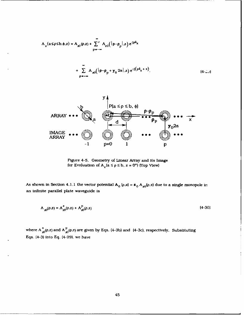
The procedure follows that of Section 4.2 and Is illustrated below. Using the notation ofFigure 4-5. the vector potential A,(a S p S b, 0. z) Is

44

A (aeprbOz) =A,(p,z) + 'A( JI I 1Z) ejp'6x

+ A,,,(IP-P + y,,29 1z) eJx') (P. +

IMIAGE 000 Oo 0-1 P=O 1 p

Figure 4-5. Geometry of i.near Array and Its Imagefor EvalJuation of Az (a g p:5 b, z 0 O+) (Top View)

As shown in Section 4. 1.1 the vector potential A0 (p,z) z z 0 Azo(p,z) due to a single monopole In

an infinite parallel plate wavegulde is

A zop.z) = Aa (p~z) + AP (p,z) (4-30)

where A a(p~z) and A P p~z) are given by Eqs. (4-3b) and (4-3c), respectively. Substituting

Eqs. (4-3) into Eq. (4-29). we have

45

A,(a:5p:b ,z)= Kp0 V0 (z=O-) n C Z[JZI

(khj

+ ) ) nb) -o a)]

+ OC ()n o H -

a Cn(z) I Jo( a) H 2)nP)- C enCn(z) I Jo( a)nuO nwO

0( cn lp -p p l) e ' 'x + H '_K o n p -p ) e -J (P 6 x + )j"y 2s- }(4-31)

where relation (4-22d) has been used. In Eq. (4-31), I' is given in terms of known currentn

expansion coefficients by Eq. (4-24a).

To Impose continuity of the total magnetic field In the coaxial aperture it Is essential to

represent the total tangential field H# (a < p < b, z = 0+) with respect to the reference element

p = 0. To that end, as in Section 4.2. with the aid of the Addition Theorem for Hankel

functions, we re-expand the vector potential Azo(Ip-p P .z) and A 0(p-pp + yO 2s Lz) in

Eq. (4-29) about a cylindrical axis centered at the reference element. The assumption of a

rotationally symmetric aperture field and use of appendix D and Figure 4-6. lets us write

* ( 1C P-P+Y2)z(K" P H (2) (K 7Ns) (4-32a)

0 P 0

* C2)(K p-pp + yo2sl)= Jo(Kjp) H o (2) K(pd) 2+ (2s). 4-32b)

46

Substituting Eq. (4-32a) Into Eq. (4-31), one obtains

A(a:5p!Kb.z) oVj(z=0-) f i)

n

b -knO l_(nn

O -]( khkh)

2

2) (2 ) K a ) ( + en ) pj

I-.o nCn(z) I:, ( n ba) -(Hc0) -0 (K Cn(z). n J(K.a) Io(cp)

XHo)Q (Knpd) Cos p8 - H(.2 (2K ns) - 2 HO'2)Knd p2 a +(\2 )Cos p8]

[= X l P=1 O d/ 8j] (4-.33)

where Eqs. (4-17b) to (4-17d) have been used. This relation can be re-written in the form

Az(a-p! bz) --- K°V°(z=f-) n C(z)~ - 1 nZ)

[_j lnp.o +Jo(K p)H5I ,K) -o HK p.Jo\ ) 4 1,J(KP) ,

47

- n Cn(z) I J 0 ( a) [H (%np) + J0 (Cp) Sn(8j] (4-34)n-0 J

Y

Field pointP(a<- p 5. b,f)

'p-pp1

p=O IpI d p-th xelement element

Figure 4-6. Triangle Pertaining to Addition Theorem

for Hankel Functions H; 1 (n I p-pp)

where the structure factor, Sn(6x) Is defined in Eq. (4-18c). It should be mentioned that, as In

Section 4.2, the first sum in Eq. (4-34) represents the aperture field contribution while the

second sum represents the probe contribution to the total vector potential in the parallel plateregion a : p < b. The first three terms in the first bracket and the first term in the second

bracket represent the self-contribution due to the element (p = 0). while the forth term in the

first bracket and the second term in the second bracket, which are proportional to Sn(8x}.represent contributions due to the rest of the array elements (I p I > 1) and all elements of the

image array. Thus, Eq. (4-34) also applies to four geometrical configurations specified by

Sn(bX) in Eqs. (4-18c) and (4-19a) to (4-19c).

The expression for H, (a < p ! b. z = 0+) can be now obtained from Eq. (4-28), which since

a/a = 0 may be written as

H (a-pb, z=0 +])= -1 OAZ(a<-p_bz=0) (4-35)

48

Substitution of Eq. (4-34) into Eq. (4-35) yields the desLed expression for the total magnetic

field in the aperture H, ta p : b, z = 01)

4.5 Active Admittance, Ya(,)

The active input admittance Ya (8 ,) is the admittance that each element sees when all array

elements are excited with the forced aperture voltage Vo (z = 0) and progressive phase factor

exp(-Jp~x ) as shown schematically in Figure 4-7. As already mentioned, 8x = kxo sin o is the

inter-element phase increment. o is the scan angle off broadside, p = 0, + 1, + 2, ... is the serial

element number where p = 0 denotes the reference element.

TEM - wavey propagation direction

dY

Vo ej 2 lx V oe j V0 Vo§jax Voe- 2 8x

Figure 4-7. Active Infinite Linear Array Pertaining toUniform-Amplitude, Linear-Phase Progression Excitation

The analysis is based on the continuity condition for the total magnetic field in the

aperture which will lead to an expression for Ya(S,) in terms of the total magnetic field in theapertjre H$ (a < p < b, z = 0+). Utilizing results from the previous section for H* (- < p 5 b,

49

z = 0*1, we obtained the desired expression for the active input admittance Ya(x) as a function

of array geometry and inter-element phasing 8,, that is, scan angle to. The procedure is

illustrated below.

For the TEM mode approximation, the field in the aperture of the feed coaxial

transmission line can be written in the form

E(p, z=O-) =Vo(z=-) e0(p) (4-36a)

H(p, z=O-) = Io(z=O-) ho(p) (4-36b)

where the transverse vector mode functions are

eo = PO I143cpl 0 b (436c)a

ho =* I (4-36d)0 2n0"

Modal voltage and current amplitudes Vo and 10 satisfy the transmission-line equations

dVo(z) -

dz -JkZo(Z) (4-37a)

diD(z) =

dz - JkYV(Z) (4-37b

where the characteristic impedance of the coaxial transmission-line Z, is

Z -Li = in b 43C y 2R a

C

with

50

- 0 - {_ (4-37d)C r

To determine the active admittance Ya(x), defined as

Y(8)=G() + jB() =(ZO) (4-38a)

continuity of the magnetic field in the aperture is imposed, that is,

H(p,z=O) = H(p,z=O-), a - p < b. (4-38b)

Consequently, one may use Eq. (4-36b), to write

H(a <_ p <b. z=0) = o(Z=0-) ho(p) (4-39a)

or

H(a < p < b. z=O) ho(p)=Io(Z=0- ) Iho(P) 12 (4-39b)

where h o Is given by Eq. (4-36d). Since H above Is entirely C-directed [H(a < p < b. z = 0) =

+oH, (a < p < b. z = 0+)] [see Eqs. (4-28) and (4-35)]. integration of Eq. (4-39b) over the coaxial

aperture domain with dS = p dp do. yields

2n b 2,, b

i-=o p=a H,(a p! bz=O)-- dS = I°(z=O) j 1 - dS (4-40a)

51

from which,

b H(ai p(b,z=O+) dp= O(Z = O- ) Inb-

Ila 2n a (4-40b)

Thus, the input active admittance can be written as

y(8 = I(z=°- ) 2n H(a< p < b, z=O+) dp. (4-41)Vo(z=O-) Vo(z=O-) In b a

In view of Eq. (4-35). the integral in Eq. (4-41) can be expressed in terms of the total vectorpotential in the aperture as

f p H1aSp5bz o+)d (a < < : b~z= +) I b

HA( ~=0 ) d /--A z p bzO~(4-42)

pMa O p=a

Consequently, substituting A, in Eq. (4-34) into Eq. (4-42), we have

b iKvO~= En£H. (a p : 5 b.z=O+) dp

•(2)Kb) -3'f J0 (Kna) nn()

-I £,n IXJo(cKa) fi{n+ i nS.( )j (4-43)nMO j

52

where the functions 3 , and H n are defined in Eq. (4-51) and (4-5), respectively. Finally,

substituting Eq. (4-43) into (4-41). the active input admittance of a coaxially-fed monopole in

an infinite linear array radiating into a semi-infinite parallel plate region Is

a 4Zo hn In bh n=0 [j2in+n Ho2 ((Kb)-n Jona) + 2S()

aa [O(nX)]~ a + n n _n lii a) + Ia~ kh

- n InJO(Kna) [In + 1. Sn(] " (4-44)n=0

All terms in Eq. (4-44) have been already defined, but for convenience we list them below:k: free-space wave number, k=2n/.

X: free-space wavelength (4-45a)

a: probe radius and inner radius of coaxial transmission line; a << Xb: outer radius of coaxial transmission line; b << X

1: probe length

d: inter-element spacing

s: distance between probe and conducting "back-plane"; s = X/4

h: height of a parallel plate waveguide (h < /2 so that only TEM mode propagates)

Zo: characteristic impedance of the free-space coaxial transmission line

Z -C IO b-60inb

0 2,- a- a (4-45b)

o : free-space intrinsic Impedance

% - =376.7 Q ~ 120 n 12

0

53

en: (Newmann's number) an integer defined by

=1, n=O

n " 2, n2 1 (4-45d)

Xn: propagation constants of radial modes in parallel plate region

/1-(h) - Imfcn1 <0 (4-45e)

Jo(rcna): Bessel function of the first kind, zero-th order and argument xnaJo(cnb): Bessel function of the first kind, zero-th order and argument KnbHo(2)(icna): Hankel function of the second kind, order zero and of argument KnaHo(2)(,Cnb): Hankel function of the second kind, order zero and of argument xnb

In: function defined as

in =Jo(xnb) - Jo(x na ) (4-450)

]: function defined as

if = H (Cb)-H (K2)(Kna)n o (n o n(4-45g)

': function defined asn

n. l iin (4-45h)

J=I: total number of terms In probe current expansion seriesljn: function defined as

54

(2j-1)X-2 21 (2J-1)X nX

21 22lin = ( (4-451)

(2J-~X _ nX 21 h

C': current expansion coefficients determined from system of equations

J

A c =B iJ= 1.2..... I--J=1 J (4-45J

A matrix coefficient defined by

_ R21,oIa(45kA i 1: Cn1~ jln a) [H(' (K a) + J.(ic a) Sn(8~J 't~1 (-4kn=O

B1 : vector coefficients defined by

B,= , 0ndo( na)[1"n + 'nSn(')] "I. (4-451)n- 0

When high accuracy for Ya(Sx) Is not required, It Is sufficient to consider a single currentterm in Eq. (4-45h). In this special case, I = J = I and consequently

I' = c in.

5 1

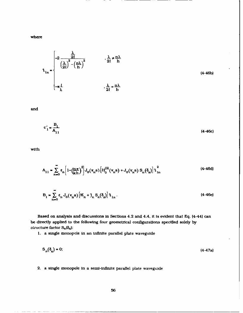
where

x-2 21 X n%

2 2 21 h

uln =(4-46b)

21 h

and

c'= BI Al I (4-46c)

with

A [nI- ) jo(ca) Ho '( a) +j 0Qca) S()J f n (4-46d)

B- nJo(n a) [9 n + n Sn(.)] "i. (4-46e)n=O

Based on analysis and discussions in Sections 4.2 and 4.4. it is evident that Eq. (4-44) can

be directly applied to the following four geometrical configurations specified solely bystructure factor Sn(8J:

1. a single monopole in an infinite parallel plate wavegulde

S n(8.) = O; (4-47a)

2. a single monopole in a semi-infinite parallel plate wavegulde

56

Sn(8.) = -H0 )'(2ns); (4-47b)

3. an infinite linear array of monopole elements in an infinite parallel plate wavegulde

Sn(8.) = 2 H(2) (Ipd) cos p8. (4-47c)p-l

4. an infinite linear array of monopole elements in a semi-Infinite parallel platewaveguide

n( =2 " Hp(nPd) cos p -H(2)(2x s)-2X H ) nd + cosp6. (4-47d)

p: Integer, denotes element number8 ,: phase increment between two neighboring elements.

The rate of convergence of I is predominantly determined by the behavior of H; (nPd)p

and p 2 + (&) for large p, which is proportional to -L. The slow convergence of

this series with respect to the index p was accelerated as described in Appendix E.

Note that Eq. (4-44) can be also applied to above mentioned four geometries with coaxially-fed annular aperture elements simply by setting I' = 0, since in this case probe length I = 0.

n

With the probe admittance, Y(8,) defined, we can now evaluate the active reflection

coefficient of the array, ra(8x), as well as the scattering coefficients between array elements.

The final two sections of this chapter show how those quantities are derived.

4.6 Active Reflection Coefficient, ra(8x)

To improve the radiation efficiency it is necessary to match the array element to the TEM

coaxial feed-line. The active reflection coefficient referenced to the coaxial aperture plane is

57

r.( Y - ( (4-48a)

Yc + Y.(81)

where YS(6,J is given by Eq. (4-44) and Y. is the characteristic admittance of the coaxial feed

line

y ( _L 4-48b)CZO

As will be shown, one can determine the probe length I' and spacing s, so that ra = 0 at a givenfrequency and a particular phasing.

In the single aperture mode approximation, the aperture field is described by a singleparameter - the total coaxial TEM mode voltage Vo given by

Vo=i I + a(.)] Vim (4-49)

where Vjc is the incident TEM mode voltage in the aperture.

4.7 Coupling (Scattering) Coefficients, SP

The coupling coefficient between two monopole elements of the infinite linear array in aparallel plate wavegulde, for example, between the reference element p = 0 and p - th element

is defined as

VPSo (4-50)

Vnc

0where V Inc is the modal voltage of the Incident TEM mode in the coaxial-feed line (p = 0) andVP is received TEM mode voltage in the coaxial transmission line of the receiving (p - th)

rec

element. All monopole elements except the excited one (p = 0) are match-terminated as isshown schematically in Figure 4-8.

58

-2 -1 P=O 1 2 p

Figure 4-8. Infinite Linear Array Pertaining to the Definitionof Coupling (Scattering) Coefficients

The coupling (scattering) coefficients SP may be related to the active reflection coefficients,defined Wi the previous section, with the usual relation

which upon Fourier inversion yields

S x/j r (k. 0) e Jko2(dk, (4-511m)

Since ra(kxo) Is an even function of kO. we write

5 Pd j F(k x) cos (k xyd). (4-52)

59

5. FAR FIELD PATTERN OF THE SINGLE MONOPOLE IN AN INFINITE AND SEMI-

INFINITE PARALLEL PLATE REGION

In this chapter we shall evaluate far-zone field Eo(p) due to a single monopole radiating

into an infinite and semi-infinite parallel plate region. Throughout this and the following

chapter It Is assumed that h < X/2, which is adequate for most practical applications. In this

case only the TEM mode propagates in the parallel plate region.

5.1 Far Field E.0(p,*) Represented in Terms of Radial Modes

The simple analysis Is based on expressions derived in the previous two chapters for the

electric field and reflection coefficient of a single monopole in an infinite and semi-infinite

parallel plate region.We begin with the expression for electric field due to a single monopole defined in Section

4.1.2 as [see also Eq. (4-9)1

E;o(p) + EP(p) (5-1)

a

where Ej and E% are defined by Eqs. (4-5c) and (4-6c), respectively. Since h < X/2, only the

n=O terms in the respective sums contribute to the far field. Therefore, in this case, one has

Eo(p) = JKVo(z=O) J Ho2 (kp), kp>>l (5-2a)

EP (p) -JKVo(z=0-) 1,Jo(ka) Ho(l(kp), kp>>l 5-2b)

and consequently,

E0(p) JKV 0(z=0-) [I - I'oJo(ka)] H2) (kp). kp>>1. (5-2c)

In Eq. (5-2), from Eqs. (4-5d) and (4-451) to (4-451) we have

60

K- 'R2h I b (5-3a)

a

Jo = Jo(kb) -Jo(ka) (5-3b)

and

JIoc- (5-3c)

where Ijo Is given by Eq. (4-451) with n = 0 and where the probe current expansion coefficients

c' are computed from the system of equations (4-45J) with Sn(8x) = 0 as given by Eq. (4-47a).

Furthermore, Vo(z = 0-) is the total voltage in the coaxial aperture cooresponding to the singleTEM mode aperture field.

After the propagating TEM mode (n = 0), the next higher non-propagating mode in theparallel plate region is TM1 (defined with respect to the radial direction) represented by then = 1 term in Eqs. (4-5c) and (4-6c). As one can see from these two relations, the radialdependence of this mode is determined by the zero order Modified Bessel function

Ko(k p V(/2h)2 - 1 ). The function Ko (x) tends to zero as x - o*. The first order asymptotic

expression for large argument is

Ko(X)- e-x. (5-4)

The (fast) expoential decay of Ko (x) vs x Justifies the single TEM mode far-zone field

approximation in Eq. (5-2).

Next we write the expression for the far field E.o(p,o) due to a single monopole in a semi-

Infinite parallel plate wavegulde. This relation can be easily obtained from Eq. (5-1) by

superimposing to It Its Image contribution, that Is.

(2l) _ (2)( p+ o2 )" -,

EO(p,0) -JKVo(Z=O)[.1o - IJo(ka)][H o (kp)-H o (kIp+y 0 2sI)].

61

Here, as seen from Figure 5-1 in the far zone

Jp+ y02 sI Ep +2s cos (5-6)

where * is measured from the y-axis, that is, x/2 - 0. Equations (5-3) and (4-451) apply here

as well. The current expansion coefficients c' are also computed from the system of equations

(4-45J) where now S n(80J is given by Eq. (4-47b) as

=,8 H (~2) (21c s). (5-7)

Par lleePa Region

For convenience we cast Eqs. (5-2c) and (5-5) into a uniformn relation

62

Eo(p, ) =JKVo(z=0)[Jo- l'° Jo(ka)][H(2 (kp)-UH(2)(k~p + yo2s 1)] (5-8a)

where U is the unit step function defined as

0: monopole in an infinite parallel plate regionu = (5-8b)=1; monopole in a semi-infinite parallel plate region

As already mentioned I' in Eq. (5-8a) is given by Eq. (5-3c) in terms oftjo and c The "tjo is0

defined by Eq. (4.451) while the c' are determined from Eq. (4-45) with S n as given by

Eq. (4-47a) for a single monopole in an infinite parallel plate region and by Eq. (4-47b) for a

single monopole in a semi-infinite parallel plate region.

When x Is large. the asymptotic approxlmatIon for the lankel function of order zero H1 (2x)

is

HO }(x )= C- -(x-4). (5-9

Consequently.

H(2(kp) - UHo ()(kp + 2ks cos')

kp e 1-U :2 i+ 2 kcosgirpek~Ji.Ukp e .(-10)

For 2ks << kp we may use

1 - x x<< 1 (5-1 la)j+x 2'

63

and then

H()(kp) - U H(2) (kp+ 2ks cos)

kp 1U=

For all practical applications s = X/4 and since kp >> 1 in Eq. (5-1 lb) ks/kp 0.

Substituting Eq. (5-1 lb) Into Ea. (5-8a), we get the far field due to a single monopole in an

infinite (U=O) or semi-infinite (U=1) parallel plate region as

Eo(p.,) =JK f Vo (z=O-) [30 -I o Jo(ka)] e-('P -4)

U=0

2J sin (ks cos ) ekl c- o; U = 1. (5-12)

The Vo (z = 0-) in Eq. (5-12) can be expressed in terms of the modal voltage of the single

TEM mode in the feed coaxial transmission line Vjn and the reflection coefficient as

v0 (Z=o-) v oJ + ra(z-oa]. (5-13)

As defined in Section 4.6. the reflection coefficient is

z -ZaZ +Z (5-14a)

a c

where Z. - I/Ya and Z, is the characteristic impedance of the coaxial feed line

64

Z C ZO(5- 14bir

with

In 1Z.i (5- 14c)Z!2nr a

The input impedance Za(z =0-) is determined from Eq. (4-44) with Sn given by Eqs. (4-47a) and(4-47b) for a monopole in an infinite and a semi-infinite parallel plate waveguide region,respectively.

5.2 Single Monopole Gain Pattern, g(e)

The normalized gain pattern is

=OPW (5-15a)

where P p. 0) and PO(P) are the power densities at p due to a mnonopole (in an infinite or a semi-

infinite parallel plate region) and an isotropic source, respectively defined as

H(- = EoH Z (5- 16ay

and

27cph

In Eq. (5- 16b), the incident power is

In Z (5-17)cn

Consequently Eq. (5-15a) becomes

65

G4 o1P_ ivC12 C o (5-18)

2xph

Substituting Eq. (5-3a) into Eq. (5-12) and then (5-12) into (5-18) we obtain an explicitrelation for the gain pattern, that is.

ffi Zc 2 1 ; =0

I Z c1 +r)[o-IJ.o(ka)]12{ (5-19)X a 4sins (ks Cos ;); U=l .

Defining the complex field pattern by

g () Re=4 h-- (1Z~ Ol+ r)[jo-VoJo(ka) ] 1U=

=h " o( 2j sin (ks cos )e''" = (5-20a)

normalized so that

Ig() 2 =G0 • (5-20b)

Now Eq. (5-12) can be expressed in the form

Ezo~,;)_1 Fl/o Vinc e"Jk' g().

2-n V Z e Y i: P- o-:p (5-21)

Note that the field of a monopole in an infinite parallel plate region Is independent of the

observation angle . The phase center of the field is at the axis of the element (x = 0. y = 0).

For a monopole in a semi-infrinite parallel plate region however, the phase of the far field vsobservation angle ;is constant with respect to the point (x = 0, y = - s). Thus in this case the

radiation pattern phase center is on the conducting plane behind the monopole.

In Appendix H we show that Ezo(p.;) as given by Eq. (5-21) satisfies the conservation of

power condition

c (1_ Ir ) = pt(5-22a)

66

where

P n Vic1 (5-22b)C

is the TEM mode incident power in the feed coaxial transmission line with characteristic

impedance Zc. The input reflection coefficient r, is given by Eq. (5- 14a) in terms of the input

impedance. which can be computed from Eq. (4-44) with Sn giver, by Eq. (4-47a) for a singlemonopole In an infinite parallel plate waveguide and by Eq. (4-47b) for a single monopole in a

sernd-infinite parallel plate waveguide. Furthermore, in Eq. (5-22a) Pt represents far fieldradiated power defined as

Pt = 2itph Re P(p) =21rph (5-23a)

for U=O. and

Pt Ref jE(,) x H*0 (p.O) p dO dz iReJ IE (pA)I 2 p dO (5-23b)

for U=1.

67

6. FAR-FIELD ELEMENT PATTERN OF AN INFINITE ARRAY RADIATING INTO AN

INFINITE AND A SEMI-INFINITE PARALLEL PLATE REGION

In this chapter we derive expressions for the far field E(e)(p) due to a singly excited

monopole element in a infinite match-terminated linear array environment radiating into an

infinite and a semi-infinite parallel plate region as schematically illustrated In Figure 6-1.

As already mentioned in the previous chapter. the distance between the parallel plates h is

less than X/2 so that only the TEM mode propagates.

The analysis is based on the relation

E __ /dE (p) = J/d E(p) d kxO (6-1)

where Ez (p) is the total far-field of the active array (all elements are excited with uniform

amplitude V0 (z = 0-) and linear phase progression 8x = kNOd = kd sin o) at an observation

point P = x o x + Yo y.

Note that E (p) as defined in Chapter 4 and F.x,y) in this chapter denote the same active

array field in the parallel plate region. The E represents the active array field in terms of

cylindrical radial modes while the E represents the active array field in terms of Floquet

modes in the unit cell. Thus, Ez(p,.) m E z (x,y) where (p,0) and (xy) refer to the same

observation point.

The analysis uses three basic steps:

(1) Obtain the far-field E,(p) by superimposing fields Ezo(p) from each individual

monopole, and, in a semi-infinite parallel plate region, Its image.

(2) To facilitate integration of Eq. (6-1, using Poisson's sum formula, we re-express Ez(p,.)

In terms of Floquet modes in the unit cell. By this means we obtain an expression fo- E,(x.y).

(3) Evaluate the Integral in Eq. (6-1) by the method of stationary phase.

We shall, of course, expand on this outline and shall analyze each of the steps in great

detail.

68

Far-field pointY 0 P(P)

Ez(e)(p )

d P

x

0 0 Vo 0 0

Figure 6-1. Infinite LAnear Array Pertainingto Single Element Excitation

6.1 Far Field of the Active Array E,(p,o) Represented in Terms of Radial Modes

For the active array excitation, that is, when all elements are excited with uniformamplitude Vo (z = 0-) and linear phase progression S. the total far field E(po) = zo Ez(p,O) can

be expressed as a superposition of contributions from an infinite number of single monopoleslocated at pp = xo pd and in a semi-infinite parallel plate region their images located atPP - Yo 2s in a parallel plate waveguide as shown in Figure 6-2.

[bhus, for kp >> 1, one may write

..jp j(p Sx+n )..)= Eo(jp-pP!)e +U E,,Eo(Ip-p p+ Yo2slI)e (6-2;aip=-0 0 =-

where as stated in Chapter 5, U Is the unit step function defined as

69

r 0; for an array in an infinite parallel plate regionU = (6-2b)1: for an array in a semi-infinite parallel plate region

and the electric far field due to a single monopole as defined in Section 4.1.2 is

E'(p) = E~o(p) + EP(p). (6-2c)

The E;a and EP are defined by Eqs. (4-5c) and (4-6c), respectively. Since h < X/2, only the n=0

terms In the respective sums contribute to the far field. Therefore, in this case

o Ho'(kk). kp>>l (6-3a)

EP (p) - -JKV 0(z=O-) I J,(ka) H(02)(kp), kp>>l (6-3b)

where as indicated we used ico = k. In Eq. (6-3), K, Jo and I' are given by Eq. (5-3) where the

probe current expansion coefficients c' are computed from the system of Eqs. (4-45j) with SA)

as given by Eq. (4-47c) for an array in an infinite parallel plate region and by Eq. (4-47d) for

an array in a semi-infinite parallel plate waveguide. This implies that the probe current in

Eq. (6-3b) is not that of a single monopole in an infinite or semi-infinite parallel platewaveguide as in the previous chapter but instead, the current on the probe in the active array

environment.

Upon inserting Eqs. (6-3) into Eq. (6-2c), and then Eq. (6-2c) into Eq. (6-2a) using

Eq. (4-17b). we obtain

E_(p,) =JKVo(z=0-) [o- IJo(ka)]

H 12 Ho'(k IP-ppl -jP8 -) -P8

LP=_ 0 P=-- 0(6-4)

70

P(p, , z)

b ~ ~ p-pp,+y 02s Pp

ARRUAY a0

IMIAGE ** (0 0*

-1 p=O 1 p

Figure 6-2. Geometry of the Linear Array and its Image forEvaluation of Ez(p,o) (Top View) (U=I case shown)

6.2 Far Field of the Active Array Ez(xy) Represented in Terms of Floquet Modes in a

Unit Cell

In the last section we determined the active array field in terms of an infinite sum over all

(real and image) array elements. We observe, however, that Eq. (6-4) is not directly applicable

in Eq. (6-1) because the relevant integral cannot be evaluated in a closed form.To avoid this difficulty we re-express Eq. (6-4) in terms of Floquet modes of a rectangular

unit cell guide with conducting top and bottom walls, and phase-shift side walls. A typical

zd

Figure 6-3. Unit Cell Geometry of an Infinite Linear Array of Coawially-fedMonopoles In a Semi-Infinite Parallel Plate Wavegulde

71

rectangular unit cell, of width d and height h. for an array in a semi-infinite parallel platewavegulde is illustrated in Figure 6-3. The desired representation is accomplished with theaid of the well know Poisson sum formulas:

2n(~)- ~n (6-5a)

where

F(m) f f(t) eJml dc (6-5b)

and

T= 2inp. (6-5c)

The analytical procedure is described below

Referring to Eq. (6-4), we first consider the sum

X~() I)eP'xH I(kp-ppj) (6-6a)

where, as can be seen in Figure 6-2,

22p-P1, xp)+ P=O+.* (6-6b)

SPapoulis, A. (1977) Signal Analysis, McGraw-Hill, New York,

72

In view of Eq. (6-5a) we now set

f(2rp) = H02 (k (x-pd) +y2)eJP x (6-7a)

in Eq. (6-5b), which, since p = T/2n. then becomes

2 + 2 2.)F(m)= J Ho°f{k Yd(x-c. ) y e (6-7b)

To evaluate Eq. (6-7b). we define a new integration variable

x - _d T = -X (6-8a)21r

from which we get

' = (x + X) 2 _ (6-8b)

d

and

dT = 2Ar dX. (6-8c)d

We now write

FMmS 21 2 e'm x (2 2-2) 2n _+'Fd)=29e 2 H (kV/-F+ y2 e- d m 2n dX. (6-9)

d0

Since

73

8X = kxod = kd sin o (6-lOa)

we find that

d d (kVX +y e (kxo+2m)XdX. (6- lOb)

Upon using the relation

k kin = k k° 2 Rtm (6-1I la)d

where the kxm are wavenumbers of Floquet modes in a unit cell, we finally obtain

F m) = 2A e x H k'( +y2 ) e""- X.d 1 (6- lb)

The Fourier integral of the Hankel function in Eq. (6-1 Ib) Is evaluated in Appendix F. The

result Is

-- T -JVMo Y

H()(kVXky2) e J dX=2e K 0 (6-12a)

where

x k- k ' Im{ KmO} <0 (6-12b)

74

Thus, from Eqs. (6-1Ib) and (6-12a) we find that

-Jkex e-JKmOyd (6-13)d KmO

Finally, upon inserting Eqs. (6-7a) and (6-13) into Eq. (6-5a) we get

(2) -P -jk e -JKoYHo)(k1P-Pp1) e - = 2 e e

-dkMp-p 'K.0 (6-14)

The same process may be applied to obtain

( J- Px -Jk x x e jlCrO(y+2s)

" Ho-)(kppp+yo2sl)e-- e (6-15jM =-00Mp-- m-oo KmO

Here

P-Pp + yo 2s= -/(x-pd)2 + (y + 2s) 2 (6-16)

Upon combining Eqs. (6-14) and (6-15) we may write

E (2) ) -Jpbx (2 JA

Ho (klpp -I) U H2)(kIp-pp+Y 0 2sI)e-

p=-o p=-o7

75

- _J'mo I: U=o=2 Y e e

d Y -J'S (6-17=- mO 2J sin xm0 s e :U= 6

Substituting this identity into Eq. (6-4) we obtain the desired expression for the active electric

far field

2KV0(z=0) [ 0- IoJo(ka)]E._(x,y) =J 0Z d

- _Jr, 'O 1oI; U =O

e -- (6-18)m=-oo mO 2JsinMOs e : U= I

Relation (6-18) represents the active array far field in terms of Floquet TEY modes

propagating in the y direction in the rectangular unit cell with propagation constants xmo

defined by Eq. (6-12b). From the result Just obtained, it is easy to see that. as expected, theactive array field is periodic in the x direction.

6.3 Element Pattern, g(e)( G

The identity

8o -d x/ e -jopdk.o (p = 0.+I ....)OP 2n E-d (6-19a)

where 8 is the Kronecker delta lets us write the expression for Elel due to the singly excitedOP z

p=O element in a match terminated array environment as

76

_(e) n/d

Ez (p) = 2j Ez(p) dko" (6-19b)

The expression for the active array far field is given by Eq. (6-18). which, for convenience, werewrite in the form

Vo(z=O) - eMmPEz(P) d T(kx°) e (6-20a;

where

T (k 0 ) j2K [)o- IJ (ka)] 1_O { Ie U =0X00 ( MO 2J sin icMo s e ;oU= -~o (6-20b)

km = xok m + Yoxmo (6-20c)

and, as already indicated

P = X0 X + Yo y. (6-20d)

Substituting Eq. (6-20a) into (6-19b), we get

C) 1/d -jkm PE (P) = J I Vo(k.o) Tm(k 0 ) e dkx0 . (6-2I,

mjm=- -- /d

To evaluate the integral in Eq. (6-21) we introduce the transformation

k =k +2_m=ku (622dM i6x d

77

whereupon

xm(kxm) =-Ik k- k = q k _2= xqu) (6-22b)

and

k ['u + y0 1 (up=kp[Ku+ Z x(u)]. (6-22c)

As a result. Eq. (6-21) transforms into

(e) n i/d+2n/d fAoE z(p)= 2 m Vo(u) To(u) e du (6-23)

2tm=--f -rd+2rm/d

where the Floquet relations Vo(kxo) = Vo(km) [since ra(kxDo) = rj,)] and Tm(ko) = To(km)

have been invoked. In Eq. (6-23) Lk = kp Is the large parameter and

rI; U=O

To(u) =J2K[Jo- IoJo(ka)] K~u) 2J sin xus e1j S;u; =1 (6-24a)

1yC)=&+Y 21-iu2 . ~ e U

W(u) -u + Y l-u 2 . (6-24b)P P

The sum over the index m in Eq. (6-23) may be further converted Into an Infinite Integral. so

that

78

^(e)E _ ToU -j()

E (p) =-k Vo(U ) e du.(6-25)

After a change of spatial variables

i= do (6-26a)P

K = Cos (6-26b)P

where n = /2 - 0. Eq. (6-24b) becomes

%y(u) = u sin + -U 2 cos . (6-26c)

The integral in Eq. (6-25) Is asymptotically evaluated by the method of stationary phase (see

Appendix G). The result is

E (p) - kL V°(u) 2(u To(u) e 4. V"(u) < 0. (6-27]

The stationary phase point u, defined by ap(u)/ i)u -0 at u = u, Iskk, 0= i (6-28a,

and consequently

'I'(u )(6-28b)

79

2 W(u) 1 <0

iu2Cos 2 (6-28c)U__ U

U=l

Substituting Eqs. (6-28) and (4-49) into Eq. (6-27) we obtain the first-order asymptotic

approximation to the far field due to a single excited monopole element In an Infinite match-

terminated array environment, that is

yEl Z , ( (6-29a)f~ik fh-V__ z C

where

F(,) j e j X I OJjQka) 1+ r(kd sin~)

{J2 sin (ks cos -) e 7-kc, = (6-29b)

The realized element gain pattern

2

Z P Inc (6-30a)

80

which, normalized to the available power Pin, = M.1 2 / Zc may now be written as

Z %

Note that the factor 2id/X represents the uniformly illuminated unit cell power gain since it is

the maximum gain (directivity) of an antenna with an area d. This Implies that I F() < 1.We denote the complex field element pattern by

e j( i & F( ). (6-31)

Consequently, Eq. (6-29) can be expressed in the form

Note that Eqs. (6-31) with (6-29b) for the element pattern g i)(-)in an infinite array

environment are exactly of the same form as the equation for the radiation pattern of the

single (isolated) element g(') given by Eq. (5-20a). However it is important to mention that

ra(kd sin ) in Eq. (6-29b) is the active reflection coefficient, while r. in Eq. (5-20a) is the

input reflection coefficient of a single element. In addition thec 'in the expression for I o inj

Eq. (6-29b) are probe current expansion coefficients of the active infinite array while the c

in the expression for I o in Eq. (5-20a) are probe current expansion coefficients of the single

monopole in the parallel plate region.

It Is known that within a "single mode approximation" the array element pattern g( )z

can be expressed simply In terms of a single (isolated) monopole radiation pattern g () and

Infinite array coupling (scattering) coefficients as

81

(e)(, )9e)I SP Cos (kdpsin (613

where SP as discussed in Section 4.7 are mutual coupling coefficients. We obtained thisrelation by comparing Eq. (5-20a) with Eq. (6-31) having in mind Eq. (6-29b). We see that

W g e(,) 1 +ra()(9zJ ^ o (6-34)

1+SO

where r (G) is the active coefficient and SO represents self reflection of the excited reference

element (p--O) in the match-terminated array environment. In Eq. (6-34) we assumed that SO is

equal to the input reflection coefficient of the single monopole fra = So in Eq. (5-20)]. thus we

neglected second order backscatterlng contributions to SO from neighboring elements. Also weassumed that the single-term probe current of the active array is the same as the one on asingle (isolated) monopole. From Eq. (4-51a)

1 +ra(O)= 1 +S O + SP cos (kdp sin 0). (6-35)p= 1

Substitution of Eq. (6-35) into Eq. (6-34) yields (6-33).

When there are no grating lobes in real space 1 g 00 can be also obtained from

le ICa~)~cs CO6-36)

where ra C) may be computed from Eq, (4-48a). Equation (6-36), which is based on the

conservation of power principle, is well known. It has also been derived below for an infinitelinear array of coaxially-fed monopoles in the parallel plate wavegulde.

We start from Eq. (6-29) which after using Eq. (H-54) can be rewritten in the form

82

=-ke _ 4 k 0 F& AQ T" cos (6-37a)

d~ k-Tf 00

since the transmission coefficient

Too =in0 (6-37b)

In Eq. (6-37b). Vinc Is the modal voltage of the incident TEM mode in the coaxial feed line(p=O). and V 00 is the modal voltage of the single-propagating (m--O,n--O) TE Floquet mode in

the unit cell [see Eqs. (H-49a) and (H-54)].

Substituting Eq. (6-37a) into Eq. (6-30a) gives the element gain pattern as

G --- kdcos2 I To 2 .0o0 (6-38)

On the other hand when only a single Floquet mode propagates n the unit cell the power

conservation principle states

itc2 y i )2 2Vt1y _ Y = I 0oo (6-39a)

00a 00

where Y I0 is the modal admittance of the (m=On=O) Floquet mode in the unit cell given by

Eq. (H-50c) as

,. _ cos00 co (6-39b)

Thus Vo 0 = P in Eq. (6-39a) represents transmitted power in the unit cell. From Eq. (6-

39a)

83

Yo(- )12)I T 00 12 0 (6-40a)

or

0 - a 1 (6-40b)

00

Substituting Eq. (6-39b) into Eq. (6-40b) and then Eq. (6-40b) Into Eq. (6-38) we obtain

-II() = k (I - I d (1-)12) co. (6-41)

from which, the relation for the element voltage gain pattern (Eq. (6-36)1 readily follows.

In Appendix H we show that the expressions for the active array field due to an infinite

array of monopoles radiating into a semi-Infinite parallel plate region satisfy theconservation of power condition which may be stated as

Pnc (1- I (8j I2)= Pt. (6-42)

Here

Pinc=Vinc 1 2YC (6-43)

is the TEM mode incident power in the feed coaxial transmission line with characteristic

admittance Yc. As Indicated in Chapter 4. r. represents the active reflection coefficient

defined by Eq. (4-48a). The Pt in Eq. (6-42) represents the far field radiated power within a

unit cell of cross section area d x h. It is given by

84

P=Re E x i yo dx dy. (6-44)d/2J 0

7. NUMERICAL ANALYSIS

Based on the preceding analysis, a Fortran TV computer program was generated to evalute

the probe current distribution, active impedance, coupling coefficients, and the far-field

element patterns. A comprehensive description of the computer program including a complete

listing and printout for the typical test case will be given in a subsequent RADC TechnicalReport. The program was run on a CDC Cyber 860 computer at the GL Computer Center,

Hanscom AFB, MA. All calculations were performed in single precision (15 significant digits

on a Cyber 860) complex arithmetic. The execution time to cnmpute the active admittance and

reflection coefficient for one scan angle, and the far-field element pattern value for one

observation angle, is 2.5 seconds. The time required to compute the coupling coefficient

between two elements of the infinite linear array is approximately 1.5 seconds. This program

requires 150 kbytes of memory.

The active admittance is computed from Eq. (4-44) using the relevant relations

[Eqs. (4-45)]. The (I x I) matrix with the elements Aj as given by Eq. (4-45k). is Hermitian andtherefore only 1(1+1)/2 matrix coefficients need to be evaluated. The series over index n in Eq.(4-45k) converges as 1/n 3 - Forty terms (n m,, = 40) were used throughout, unless otherwise

stated. The Sn(8,) in Eq. (4-45k) is computed for the desired geometry from Eqs. (4-47a) to

(4-47d). The series I in Eqs. (4-47c) and (4-47d) converge ae 1/4 for p -4 oo. The slowp

convergence of these series was accelerated as described in Appendix E, based on the relation:9

2 H;0(2yp)cos (2xp) =-1 +J2 (ln!Y+ )+J 1--- y2

+J mL / + 1 2_S (m+x -9 + 2 (m-x) 2 -9 y2- -(7-1)

T Tnfeld , L. at al (1974) On some series of Bessel functions, J. Math. and Phys., 26.2-,

85

valid forO0 < x< 1. In Eq. (-11mI (m±x) -, ]12 0. and y= 0.577... is the Euler constant.

The new series X converges as 1/m 3 .m

The inner products 'i in Eq. (4-45 k) were computed from Eq. (4-451).The zero-order Bessel and Hankel functions in the expression for Aij were evaluated by the

usual numerical methods.1 0 The computational accuracy of these functions was better than

10 significant digits.

The coefficients B, are computed using Eq. (4-451).

The monopole current density expansion coefficients were solved from Eq. (4-45J) using

Gauss's elimination method. Ten current terms (1=10) were used in numerical evaluationunless otherwise indicated.

The relative convergence phenomenon 1 ' was observed by monitoring the current

expansion coefficients and the active admittance value as a function of the number of parallelplate radial modes n . and of the number of current terms I. It was found that for a stable

solution it is necessary to impose the condition

I < I n .(7-2)h In=

For example if nm. = 20 and h = 0.369, one requires I<5 for 1= 0.17, 1<10 if 1= 0.2). and l<16

if I = 0.3X,. If I increases beyond these values, the numerical values for Y. tend to become

progressively less accurate. This can be seen from Figures 7-1 and 7-2 which show the activeinput conductance and susceptance at broadside scan for an infinite array radiating into asemi-infinite parallel plate region (U = 1) vs the number of monopole current terms for fourprobe lengths: 1 = 0. IX, I = 0.2X, I = 0.3X, and I = 0.233X (matched case). One also observes that

for short monopoles a single current term yields a good approximation to the active

admittance. It was found that for all four possible array geometries [Eqs. (4-47a) to (4-47d)].the plots Y, vs I exhibit a similar behavior.

10 Abramowitz, M. and Stegun, I-A. (1964) Handbook of Mathematical Functions, UnitedStates Department of Commerce. National Bureau of Standards, Applied Mathematics. 55.11 Lee. S.W.. Jones, W.R. and Campbell. J.J. (1970) Convergence of numerical solution of iristype discontinuity problems, Antennas and Propagation Symposium Digest, Columbus. Ohio.

86

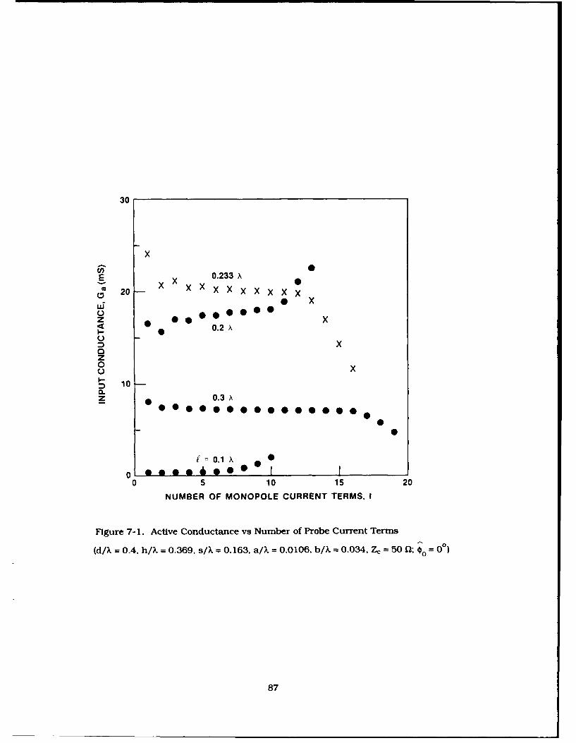
30

x0.233 A 0

j 20 X X X X X X X

0x

z 0O - x0.2A

0z0

k-10a.z 0.3A

.o1 x0

0 5 10 15 20

NUMBER OF MONOPOLE CURRENT TERMS, I

Figure 7-1. Active Conductance vs Number of Probe Current Terms

(d/% = 0.4, h/. = 0.369. s/X = 0.163, a/X = 0.0106, b/X = 0.034. Z, = 50 Q :o = 00)

87

20

0.2 X

E10 0m = 0.1x,

UT 000 0 0z

0.233 x

X0o- X X X X X X X X X X

0. X 0z 0 00 0 OO0 oo

0o XX0.3 A

10-10 I I I0 5 10 15 20

NUMBER OF MONOPOLE CURRENT TERMS, I

Figure 7-2. Active Susceptance vs Number of Probe Current Terms

(dlX = 0.4, h/X = 0.369, s/X = 0.163, a/X = 0.0106, b/X = 0.034. Z, = 50 Q; OP

With n max = 40 and ten current terms (I = 10) in the probe current expansion the active

admittance was computed with an accuracy of better than four significant digits. If a highdegree of accuracy of Ya Is desired, more current terms are needed and n max must be increased

according to Eq. (7-2).The active reflection coefficients r8 (k xO) are computed from Eq. (4-48a).

The probe current distribution has been computed based on Eq. (4-20a) . From Eqs. (4-20a)

and (4-24b), the probe current is

88

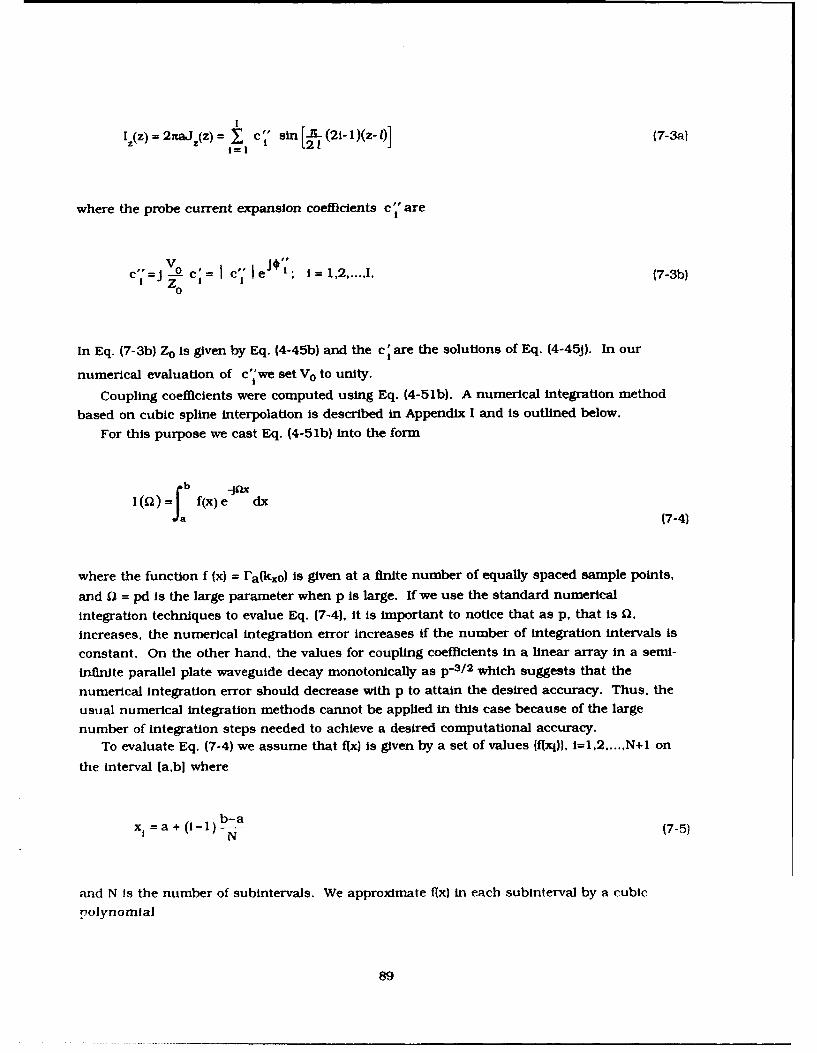
1(z) = 2_-aJ(z) c, sin (21-1)(z- )] (7-Sal1=21

where the probe current expansion coefficients c " are

ct = j cV 0 I= I c" I ; i .. I. (7-3b)" ZO c Ci

In Eq. (7-3b) Zo is given by Eq. (4-45b) and the c are the solutions of Eq. (4-45J). In our

numerical evaluation of c 'we set V o to unity.

Coupling coefficients were computed using Eq. (4-51b). A numerical integration method

based on cubic spline interpolation is described in Appendix I and is outlined below.

For this purpose we cast Eq. (4-51b) into the form

f(x) e dx(7-4)

where the function f (x) = ra(kxo) is given at a finite number of equally spaced sample points,

and 5) = pd is the large parameter when p is large. If we use the standard numerical

integration techniques to evalue Eq. (7-4), it is important to notice that as p, that is Q).

Increases, the numerical integration error increases if the number of integration intervals is

constant. On the other hand, the values for coupling coefficients in a linear array in a semi-

infinite parallel plate waveguide decay monotonically as p-3/ 2 which suggests that the

numerical integration error should decrease with p to attain the desired accuracy. Thus. the

usual numerical integration methods cannot be applied in this case because of the large

number of Integration steps needed to achieve a desired computational accuracy.

To evaluate Eq. (7-4) we assume that fix) is given by a set of values (f(xj)), I=1,2.....N+1 on

the interval [a,b] where

b-ax =a+ (1-1) N (7-5)

and N is the number of subintervals. We approximate fix) in each subinterval by a cubic

polynomial

89

3Pi(x ) = Anixn (7-6)

n 0

where coefficients A nj are determined in Appendix I by the method known as cubic spline

interpolation. Based on that one may write

rb N 3f(x)e-Jnx dx An e dx (7)7

il n=0 (7-7

where the integrals can be evaluated in a closed form. Thus the integration error is due only

to the approximation of fix) in each subinterval by a plecewise-cube polynomial PI(x). The

small interpolation error is estimated in Reference 12. In evaluating the coupling coefficients

by using Eq. (4-51b) we set N=300, which enabled us to compute efficiently values for coupling

coefficients below - 65 dB without noticeable error.

The integration routine was tested using Eq. (4-51b) with ko--G, that is.

r S p. (7-8)

Truncating the series at IpI= 50, it was found that this Identity holds within approximately

three significant digits.

The field (voltage) element patterns of the excited element (p=O) were calculated according

to Eqs. (6-31) using Eq. (6-29b), and were normalized to the unit cell gain (2 71 d/X) 1 / 2 .

12 Conte, S.D. and de Boor. Carl (1972) Elementary Numerical Analysis, McGraw-Hill. NewYork.

90

8. NUMERICAL RESULTS AND DISCUSSION

The active impedance, active reflection coefficient, coupling (scattering) coefficients, probe

current distribution, and element patterns were computed for representative values of array

parameters to show the significant trends. Most of the numerical results refer to monopole

elements with a 50 ohm characteristic impedance of the corresponding feed-transmission line

As already mentioned, field amplitude (voltage) element patterns were normalized to the unit

cell gain (2ind/.)'j2. Unless otherwise stated, in numerical computations we used 40 wavegulde

modes (nmax = 40) and 10 monopole current terms (I = 10) in Galerkin's procedure.

The results are grouped according to array structure factor Sn(8,) as defined by Eq. (4-47).

We discuss: (1) a single monopole in an infinite parallel plate region; (2) a single monopole in

a semi-Infinite parallel plate region: (3) an infinite linear array of monopole elements in an

infinite parallel plate region: and (4) an infinite linear array of monopole elements in a semi

infinite parallel plate region.

8.1 Single Monopole in an Infinite Parallcl Plate Region

Figures 8-1 and 8-2 show input conductance and susceptance, respectively, of a single

monopole in an infinite parallel plate region vs probe length I for three heights of parallel

plates, h/A. = 0.3, h/X = 0.35 and h/A. = 0.4. The feed-coaxial line has an air dielectric and a

characteristic Impedance of 50 ohms. The coaxial conductor dimensions are a/X = 0.016,

b/X = 0.037.

It is observed, from Figure 8-1. that the input conductance is very sensitive to the probe

length I and almost insensitive to the separation between the two parallel plates h. In fact, for

values I/A. ! 0.2, the conductance is practically independent of h. The same observation also

applies to the susceptance shown in Figure 8-2. From these two figures one also sees that for

short probes, I/X < 0. 1, the admittance Is a linear function of the probe length. This is because

Ya I z(z=O) and, as will be discussed, for short probes, the current distribution is proportional

to the probe length. Both curves, Ga and Ba exhibit resonant behavior at /X = 0.25. From

Figure 8-2 it is seen that for I/X < 0.25 the input admittance is capacitive, for I/X > 0.25 it is

inductive, and, for I/X - 0.25, passes through resonance.

91

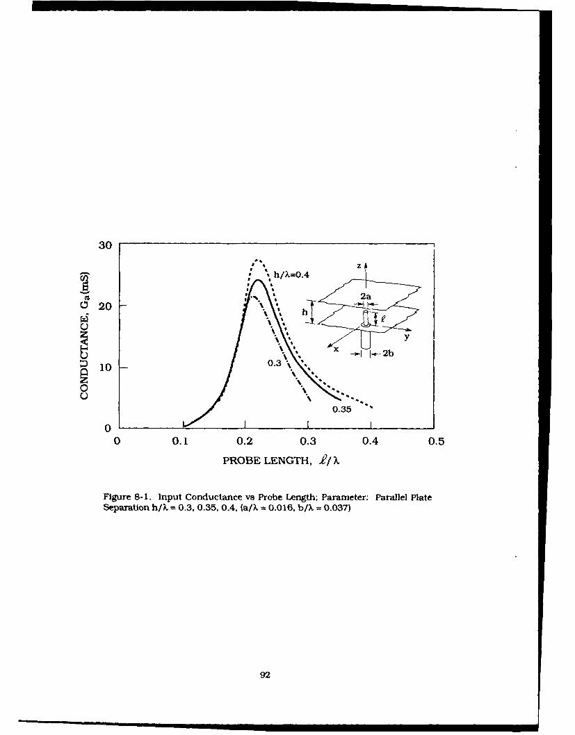
30

; h/X=-0.4

~20 hj 2

x 2

00.3

0

0 0.1 0.2 0.3 0.4 0.5

PROBE LENGTH, elk

Figure 8-1. Input Conductance vs Probe Length;, Parameter: Parallel PlateSeparation h/X 0.3. 0.35.,0.4, (a/X = 0.0 16. b/% 0.037)

92

30

2a

V)20 Ih/X,=0.4

X .- I 2b

0.35 '

~ 0

10

-10 I I I I

0 0.1 0.2 0.3 0.4 0.5

PROBE LENGTH, ii/X

Figure 8-2. Input Susceptance vs Probe Length; Parameter: Parallel PlateSeparation h/k = 0.3, 0.35. 0.4. (a/, = 0.016, b/?, = 0.037)

It should be mentioned that the analysis presented breaks down when the probe extends

very close to the top plate, that is. when I-- h. This is because in the analysis we assumed asine expansion for the probe current; hence we forced the current to be zero at the tip of theprobe. However, this is not true when I -- h because of the displacement current flowingthrough the capacitance between the tip of the probe and top plate of the guide. By monitoringthe behavior of the inptit impedance vs I/h. we loiznd that the analysis is valid for 0 S /h ,

0.99.When the parallel plate separation is greater than a liall-wavelength, higher radial modes

propagate in the guide. Figure 8-3 shows input allit lance vs prolbt, length for h,/X = 0.95. inthis case two radial modes, n=0 CTEM) and : I'M 7 ) prol)agate.

9:1

000

66

6 II.0

00

0

66

LO66N Tl

0

0 0

(Stu) V3NV.LWCIV

94

Curves Ga and Ba vs I exhibit double resonance behavior. The first resonance occurs at1/k - 0.25, and the second, as expected, at L/X - 0.25 + 1/2 = 3/4. We choose to present the

admittance curve for h/X = 0.95 because at this particular plate separation and //X = 0.75 the

reflection coefficient is zero (ra = 0). To avoid the relative convergence phenomenon, we staywithin the range allowed by Eq. (7-2), and use 1=1 for 0 < l/X < 0.05, 1=3 for 0.05 <1/k < 0.1, 1=5for 0.1 < l/% < 0.2 and I=10 for 0.2 < l/k < 0.3 with nmax--60. In the region 0.3 1/k <, 0.95 weused 1=10 and nmx=40.

In most practical applications it is useful to know the optimal separation of the parallelplates and probe length so that the monopole is matched to the coaxial feed line at aparticular center frequency fc. For this reason Figure 8-4 displays the contour plot of the

magnitude of the reflection coefficient vs h and L One sees that for h/k = h,/X = 0.35 and l/k =

L/X = 0.24,

the reflection coefficient is zero, that is, a monopole element in an infinite parallel plate

region is matched to the coaxial-feed transmission line.

0.4

~~0.4

0.24 -- 0.05

S 0.2

0.1 [ i

0.2 0.3 0.35 0.4 0.5

PARALLEL PLATE HEIGHT, h/.

Figure 8-4. Reflection Coefficient (Contour Plot of Magnitude) vsParallel Plate Separation and Probe Length, (a/X = 0.016, b/X = 0.037)

95

For this case (h,/A = 0.35). Figure 8-5 shows input Impedance vs probe length. The Smith

chart normalization is ZN = 50 ohms. Note that for 1/1 = 0.24, VSWR = I (reflection coefficient

1a = 0) and for 0.2 < I/X <0.3, the VSWR < 2.

1.0

-2.0

hj

-- 03a 2b 0.25 0.3

0 of t g2. n at e t

0.2 .

0.05

0.15

-1.0

Figure 8-5. Input Impedance vs Probe Length,(h/X = 0.35, a/X = 0.016, b/X = 0.037. ZN = 5012)

The Input Impedance vs frequency plot In Figure 8-6 allows us to assess the frequency

bandwidth of the single coaxtally-fed monopomle element. As one may note. the frequency

bandwidth corresponding to a VSWR of 2:1 is approxImately 40 percent.

96

1.0

-0.5 2.0

0-1.00 .03 1.16 \ , \

0.833 fjr 1.3/

0/, = 0.24. a/X, = 0.016 b/, = 0.037,ZN =50 f)

Figure 8-7 shows the dependence of input impedance on probe radius, a. The radius of

the outer coaxial conductor Is b = 2.3 a, so that in all cases the characteristic impedance of

the coaxial feed lines Zc 50 ohms. It is seen that the influence of these parameters on

input admittance is practically insignificant.

97

1.0

30

20z

0

Fl

I I

0

0.01

0.02

0.03

0.04

PROBE RADIUS,

a/X

Figure 8-7. Input Admittance

vs Probe Radius,

(h/ = 0.35,

1/ = 0.24, b/X = 2.3 a0X .Z3 =

0

The numerical computation of the probe current distribution based on Eq. (7.3) has also

been carried out. In our numerical evaluation of c' we set Vo(z=-0) = 1 V for the aperturevoltage in the coaxial feed line.

Figure 8-8 shows the magnitude of the current vs z/X for three probe lengths /X = 0.1. 0.2,

and 0.3. For each case two curves are plotted: the dashed line represents the probe current

distribution for a single current term 1I = 1 in Eq. (7-3a)) and the solid line represents the

probe current distribution with ten current terms 11 = 10 in Eq. (7-3a)]. It is seen that thecurrent along the probe has a basic sin k(z - 1 variation. For short probes (1/k < 0. 1) the

magnitude of the probe current Is almost a linear function of z. This Is expected since

sin k(z - 0 = k( z - 1) when 1/% < 0. 1.

98

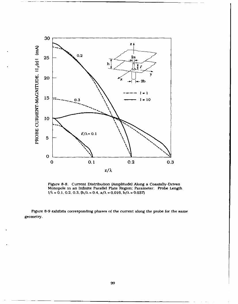
30z

- 250.2

2a20tx - -I-2b

1=10It1

10

0 0.1 ZX0.2 0.3

Figure 8-8. Current Distribution (Amplitude) Along a Coaxially-DrIvenMonopole in an Infinite Parallel Plate Region; Parameter: Probe Length10. = 0. 1, 0.2, 0.3. (h/k = 0.4. a/k 0.016, b/X = 0.037)

Figure 8-9 exhibits corresponding phases of the current along the probe for the samegeometry.

99

900.1

60 1 =10

n 0.2 z

2a

0 h"

.)-30 xi-03-. 2b

S-60

-90 10 0.1 0.2 0.3

z/X

Figure 8-9. Current Distribution (Phase) Along a Coaxially-DrivenMonopole in an Infinite Parallel Plate Region: Parameter: ProbeLength VX= 0.1. 0.2, 0.3, (h/X = 0.4, a/X = 0.016. b/X = 0.037)

It Is Interesting to note that since the probe current across the aperture (z = 0) iscontinuous, one can approximately determine the input admittance simply from

Y = I I(z-o+)

a Vo(z=O-) (8-1)

where we assumed that the probe current at z = 0 Is the same as that of the TEM mode in thecoaxial feed-line. Setting v o(z=0-) = IV in Eq. (8-1) we obtain

100

Y = (z=O )a IV (8-2)

In Table 8- 1. for the geometry of Figures 8-8 and 8-9, we compare results for the input

admittance obtained from Eqs. (4-44) and (8-2). In both cases, I = 10 and nna. = 40. As one

may see, the difference between these two results is less than 1 percent, which substantiates

the single mode approximation for the field in the aperture.

Table 8-1. Comparison Between Results Obtained fromEqs. (4-44) and (8-2) for Input Admittance Ya = Ga + JBa;Parameter: Probe Length VIX = 0.1, 0.2, 0.3.(h/X = 0.4, a/. = 0.016, b/X = 0.037)

Ya from Eq. (4-44) Ya from Eq. (8-2)

L/X Ga B. Ga Ba

mS mS mS mS

0.1 0.511 9.642 0.502 9.801

0.2 20.710 20.034 20.654 20.041

0.3 9.473 -2.732 9.471 -2.856

The probe current expansion coefficients c " as given by Eq. (7-3b) are tabulated in Tables

8-2, 8-3 and 8-4 for probe lengths I/X = 0. 1, 0.2, and 0.3, respectively. In each case coefficients

are given for the single (I = 1) and ten (I = 10 ) current terms in Eq. (7-3a).

Table 8-2. Probe Current Expansion Coefficients;Parameter: Total Number of Current Terms I = 1, 10,( .X = 0. 1, h/X = 0.4, a/4 = 0.0 16, b/X = 0.037)

1=1 1=10

i 1c " I cmA D% mA Dg8.222 -93.26 8.566 -93.76

2 0.201 112.753 0.697 -93.024 0.033 -133.465 0.279 -93.336 0.041 -107.547 0.161 -93.648 0.044 -101.629 0.120 -94.0410 0.074 -97.74

101

Table 8-3. Probe Current Expansion Coefficients;Parameter: Total Number of Current Terms I = 1, 10,(1/k = 0.2, h/. = 0.4. a/ = 0.016, b/X = 0.037)

Il c=I0mA mA

1 27.623 -132.37 28.369 -141.272 2.050 167.403 1.406 -131.424 0.575 178.175 0.592 -132.766 0.303 -176.537 0.341 -134.168 0.195 -172.999 0.227 -135.3610 0.13 9 -170.34

Table 8-4. Probe Current Expansion Coefficients;Parameter: Total Number of Current Terms I = 1. 10,(I/X = 0.3. h/X = 0.4. a X = 0.016, b/X = 0.037)

1=1 I=10

I I 110IimA DeS. mA Deg.

1 14.341 139.43 12.479 141.352 3.155 97.283 0.329 -135.174 0.752 101.785 0.133 -146.526 0.368 103.337 0.074 -156.178 0.224 104.349 0.048 -164.8010 0.153 105.12

Figures 8-10 and 8-11 show the magnitude and phase, respectively, of the probe current, forthe geometry of Figure 8-6. that is, h,/X = 0.35. and /L = 0.24. In this case. as Indicated, the

monopole is matched to a 50 l coaxial feed line. One may see from these two figures that, asexpected, the magnitude of the probe current at z = 0 Is 20 mA and the phase Is zero, that Is

Iz = 0 + ) = 0.020 A.

102

30

25a

O 20 1

%- Hx-2b

15

~10

U%

0 .5

00 0.1 0.2 0.3

z/k

Figure 8-10. Current Distribution (Amplitude) Along aCoaxlally-Drlven Monopole In an Infinite Parallel PlateWaveguide: Parameter: Total Number of Current Terms 1 1.10, ( /X = 0.24, h, /X = 0.35. a/X = 0.016, b/X = 0.037)

103

0z

1=1 2a-10 10

hJ

i-20 y

-3O0 0.1 0.2 0.3

z/X

Figure 8-11. Current Distribution (Phase) Along aCoaxially-Driven Monopole In an Infinite Parallel PlateWaveguide; Parameter: Total Number of Current Terms I = 1,10, (1, X = 0.24, hJ/2 = 0.35, a/2. = 0.016, b/;. = 0.037)

The respective coefficients in the expansion for the probe current are tabulated in

Table 8-5.

Table 8-5. Probe Current Expansion Coefficients;Parameter: Total Number of Current Terms I = 1, 10,(L/X = 0.24, hc/X = 0.35, a/X = 0.016, b/X = 0.037)

1=1 1=10

1c' Ic', p

mA Dn. mA1 25.2M ' 174.56 21.671 169.092 3.075 120.913 0.785 -164.334 0.782 127.025 0.339 -167.856 0.390 129.827 0.190 -171.348 0.240 131.799 0.134 -174.2410 0.165 133.32

104

Figures 8-12 and 8-13 show the amplitude and phase of the probe current for h/X --0.95.I/X = 0.75. From Figure 8-3 one sees that for this geometry Ya = 20 mS, that is, in this case, themonopole is also matched to a 50 Q2 coaxial feed-line. The curve I I,(z) I exhibits a typical

double maximum variation vs z since 1/2 < I/A. < 1. Note that the second maximum (z = X/2) islower than the first maximum (z = 0) which is also typical for a long dipole antenna driven

from a coaxial line. The respective coefficients in the probe current expansion are tabulated

in Table 8-6.

30

25 2a

20 y--V j - 2b

10

3 15 -

10 -

W 5 -

0- ---- - - - - - - - - - -

00 0.1 0.2 0.3 0.4 0.5 0.6 0.7 0.8

z/,%

Figure 8-12. Current Distribution (Amplitude) Along aCoaxially-Driven Monopole in an Infinite Parallel PlateWavegulde; Parameter: Total Number of Current Terms I = 1.10, (1/k = 0.75, h/?. = 0.95, a/X = 0.016, b/k = 0.037)

105

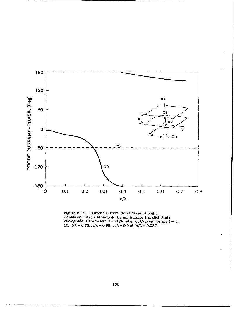
180

120

2a

0 y-p- x 2b

'0

-120 10

-1800 0.1 0.2 0.3 0.4 0.5 0.6 0.7 0.8

z/X

Figure 8-13. Current Distribution (Phase) Along aCoawdally-Drlven Monopole in an Infinite Parallel PlateWavegulde; Parameter: Total Number of Current Terms I = 1.10, (I/, = 0.75, h/%, = 0.95, a/fi = 0.016. b/X = 0.037)

106

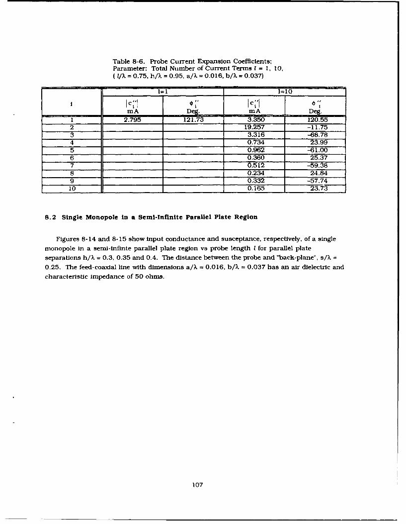
Table 8-6. Probe Current Expansion Coefficients;Parameter: Total Number of Current Terms I = 1, 10,(I/% = 0.75, h/X = 0.95, a/k = 0.016, b/% 0.037)

1=1 1=10c "I € 11 c 'i""!t*t

mA De . mA Deg.

1 2.795 121.73 3.350 120.552 19.257 -11.753 3.316 -68.784 0,734 23.995 0.962 -61.006 0.360 25.377 0.512 -59.38

8 0.234 24.849 0.332 -57.7410 0.165 23.73

8.2 Single Monopole in a Semi-Infinite Parallel Plate Region

Figures 8-14 and 8-15 show input conductance and susceptance, respectively, of a single

monopole in a semi-infinte parallel plate region vs probe length I for parallel plate

separations h/X = 0.3. 0.35 and 0.4. The distance between the probe and "back-plane". s/X =

0.25. The feed-coaxial line with dimensions a/X = 0.016, b/X = 0.037 has an air dielectric and

characteristic Impedance of 50 ohms.

107

30

wa '

20 --

o ' I

~10

0.50.3 0.35

0 1

0 0.1 0.2 0.3 0.4 0.5

PROBE LENGTH, P/.

Figure 8-14. Input Conductance vs Probe Length;Parameter: Parallel Plate Separation h/k = 0.3, 0.35,0.4, (a/% - 0.016, b/.X = 0.037, s/X = 0.25)

108

30

z

~.20 -

E 2b

U 10

h/X=0.4U 0.3 0.35 -.

0 - - - - - -

-10 I0 0.1 0.2 0.3 0.4 0.5

PROBE LENGTH, i/PX

Figure 8-15. Input Susceptance vs Probe Length;Parameter: Parallel Plate Separation h/X = 0.3, 0.35,0.4, (a/X = 0.016, b/X = 0.037, s/X = 0.25)

it is observed, from Figures 8-1, 8-2, 8-14, and 8-15 that for the short probes (1/X < 0.1) theinput conductance and susceptance of the single monopole in a semi-infinite parallel platewaveguide is practically the same as that of a single monopole in an infinite parallel plateregion. This is expected because a short probe radiates very little power into the parallel plateregion. Consequently, for a monopole in a semi-infinte parallel plate waveguide, coupling ormutual interaction between the probe and its image is small. As probe length increases, thecurves for conductance and susceptance in Figures 8-14 and 8-15 slowly depart from those inFigures 8-1 and 8-2. The difference is due to mutual coupling between the probe and its image.

As for a single monopole in an infinite parallel plate region, one sees from Figures 8-14

and 8-15 that the input admittance of a single monopole in a semi-infirte parallel plate

region Is very sensitive to probe length ( 1) and almost independent of the distance between ,iW'wo parallel plates (h). Here also, curves Ga and Ba exhibit resonance at approximately 1/k0.25. It is seen from Figure 8-15 that for 1/k < 0.25 the input admittance is capacitlv- Fr I

109

0.25 it is inductive, and for 1/k a 0.25, it passes through resonance.For practical design applications. Figure 8-16 displays the contour plot of the magnitude of

the input reflection coefficient vs the probe-ground distance (s/X) and probe length (Ifi..) for h/XL= 0.35. It Is seen that for 9/k = s,/k 0.227 and 1/X = /X= 0.219. the reflection coefficient iszero. Thus a single monopole radiating into a semi-infinte parallel plate region is matched tothe 50 ohm coaial-feed line. It was found that for any h/)L one can find a corresponding sc/kand 1 /X so that the Input reflection coefficient r, = 0.

0.4z

ee 0.3 2

z

0.20.

0.1 0.2 0.227 0.3 0.4

PROBE GROUND DISTANCE, s/X

Figure 8-16. Reflection Coefficient (Contour Plot ofMagnitude) vs Probe-Ground Distance and ProbeLength (h/). = 0.35, a/X = 0.0 16. b/k = 0.037)

110

Input Impedance vs probe-ground distance (dashed curve) for I/X = 0.15, 0.2, 0.25, and 0.3 an-,vs probe length (solid curve) for s/X = 0.15, 0.2. 0.25, and 0.3 is shown in Figure 8-17. TheSmith chart normalization ZN = 50 ohms. Note that although impedance is more sensitive te

I/X than s/X, the curves 1I/ = const and s/X = const are approximately orthogonal. Thisproperty Is useful in determination of /X and s,/k which correspond to a point ra = 0.

1.0

0.

-..0i jo 0.02.25o

0.2 0.3

s/X =const 2.0X/ =-const!

-0. 5 _R/ X=-1.5 -2. 0

-1.0

Figure 8-17. Input Impedance vs Probe-Ground Distance andProbe Length, Wh/X = 0.35, a/k = 0.016, b/X = 0.037. ZN = 50 Q)

Figure 8-18 shows input impedance vs probe length for s,/% = 0.2275 (soid curve) and inpu.impedance vs probe-ground distance for l /X = 0.2 187 (dashed curves). The two curves intersect

at the point r, = 0 since as already mentioned for 9,/.k 0.2275, ,/X = 0.2 187 the mnonopole

input Impedance is 50 ohms.

1.0

-1.00

-112

For the same case (LJX? = 0.2187, s,/X =0.2275). Figure 8-19 shows input Impedance vs

frequency. It Is seen that the frequency bandwidth corresponding to a VSW~R of 2:1 isapproximately 40 percent.

2.

0.5

Fiue81.IptIpdnevzrqec hX .5

k.h=.17 (X.=0.25 /(=001.b/.=007 N=5

11

Figure 8-20 shows the dependence of input impedance on probe radius (a). As in Section

8.1. the radius of the outer coaxial conductor is b = 2.3 a. so that in all cases the characteristicimpedance of the coaxial feed lines Zc = 50 ohms. From this figure It Is seen that Input

admittance is almost independent of probe radius for a/ > 0.01.

30

20

z

s y

-10 I I

0 0.01 0.02 0.03 0.04

PROBE RADIUS, a/X

Figure 8-20. Input Admittance vs Probe Radius (h/X = 0.35.S/X = 0.2275, //X = 0.2187, b/X = 2.3 a/k, ZN = 50 Q2)

Based on Eq. (7-3). Figures 8-21 to 8-25 show the amplitude and phase of the probe current.The dashed curve represents the probe current distribution for a single current term [I = 1 In

Eq. (7-3a)] and the solid curve represents the probe current distribution with ten current terms

I = 10 in Eq. (7-3a)]. The aperture voltage in the coaxial feed-line [see Eq. (7-3b)] isVo(z = 0- = I V.

114

30 90

PHASE - 60

N hIj20 30

70 -- AMPLITUDE 1=0-30

5 - -60

0 l I[-900 0.1 0.2 0.3

z/X

Figure 8-2 1. Current Distribution Along a Coaxially-DrivenMonopole in a Semi-Infinite Parallel Plate Region.(h/X. = 0.35. i/X = 0.15. s/X = 0.15. a/I, = 0.016. h/I). 0.037)

115

30 90

25 4~60N

A

j20 -x -- *2a 30

15 ---- I0

I=10

10 -APrUE--30w

o 5 :-------- -60

PHASE

0 -900 0.1 0.2 0.3

Z/%

Figure 8-22. Current Distribution Along a Coa.-dally- DrivenMonopole in a Semii-Infinite Parallel Plate Region.(h/k = 0.35, 1/X = 0.3. 9/X = 0. 15, a/X = 0.016. b/X = 0.037)

116

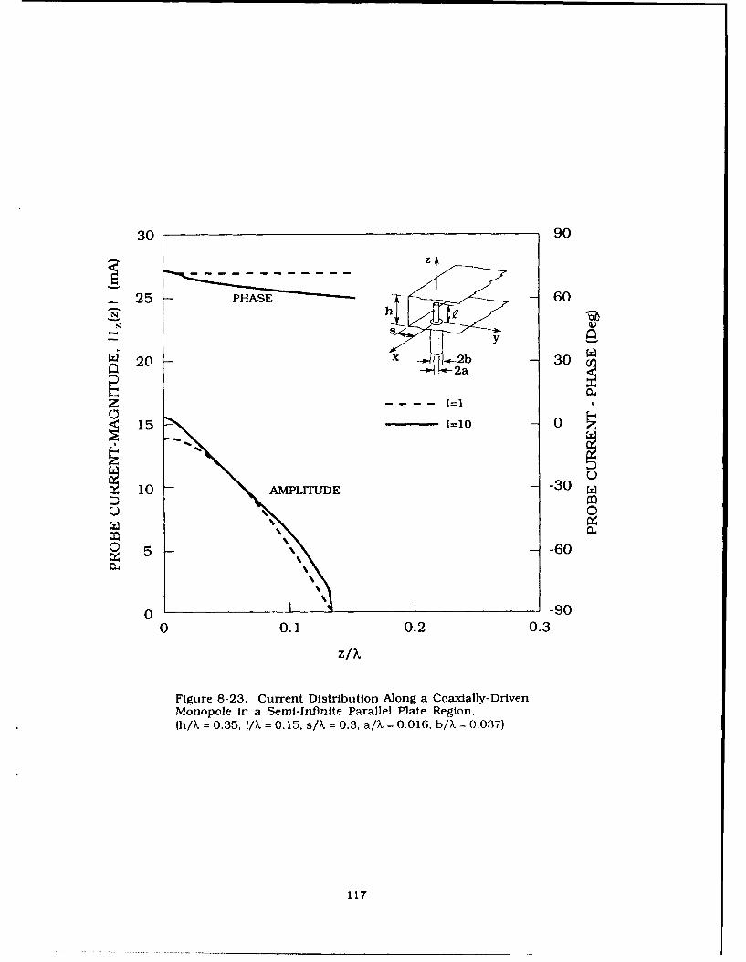
30 -90

25 PHS 60N s

y

W 20 -x -. I.2 30-1-2a

15 -1=100

10 APU E-30oWo %

54 -60a44

0 -900 0.1 0.2 0.3

Z/%

Figure 8-23. Current Distribution Along a Coaxially-DrivenMonopole in a Senfl-Infinite Parallel Plate Region.(h/k = 0.35, 1/X = 0. 15, sIX, = 0.3. aIX = 0.0 16. b/X =0.037)

117

30 90

- 25 60

y

120 x -, w-b30

~15 0-- =1=10

U

AMPLITUDE-0

0'1 7 -900 0.1 0.2 0.3

z/k

Figure 8-24. Current Distribution Along a Coaxially-DrivenMonopole in a Semi-Infinite Parallel Plate Region,(h/k = 0.35, VA = 0.3, sAX = 0.3, aAX = 0.016, bAX = 0.037)

118

30 90z

- 25 - AMPLITUDE hY f2 60

_ s

S20 2a30

Z I=10

S150

10 3

o %

5o -60

0 11-j-900 0.1 0.2 0.2187 0.3

z/X

Figure 8-25. Current Distribution Along a Coaxially- DrivenMonopole In a Semi-Infinite Parallel Plate Region. (h/X = 0.35,LJX = 0.2187, s,/X = 0.2275, a/k 0.016, b/?, = 0.037)

Figures 8-21 to 8-24 present current distribtulon along the probe for s/k 0. 15. 0.3 and I/".=0. 15, 0.3. Notice that as in Section 8.6 for the short probes (1/X < 0. 15) a single current term

in (7-3a) approximates the total probe current fairly well while for 1/k > 0.15 more terms are

needed.Figure 8-25 exhibits probe current variation vs z/X for the mnonopole matched(sf,=0.2275, L /X 0.2187) to a 50 ohm coaxial feed-line. Not~ce that, as expected, at

Z-=0o IIlz(z =-0 +) 20 mA and the probe current phase is zero.

119

For the same geometries the probe current expansion coefficients c'; as given by Eq. (7-3b)

are given in Tables 8-7 to 8-11. In each case coefficients are given for the single (I = 1) and ten

(I = 10) current terms in Eq. (7-3a).

Table 8-7. Probe Current Expansion Coefficients;Parameter: Total Number of Current Terms I = 1. 10,(h/X = 0.35, I/X = 0.15. s/ = 0.15, a X = 0.016, b/X = 0.037)

1=1 1=10

II c i'l Ii Ic ;'l 'mA De_.mmA De.

1 16.498 -10093 17.940 -103.392 0.523 -152.863 1.155 -100.69

4 0.197 -131.88

5 0.471 -101.176 0.121 -124.417 0.264 -101.648 0.085 -120.549 0.172 -102.0510 0.065 -118.08

Thble 8-8. Probe Current Expansion Coefficients:Parameter: Total Number of Current Terms I = 1, 10,(h/X = 0.35, I/k = 0.3, s/?, = 0.15, a/X = 0.016, b/k = 0.037)

1=1 1=10

mA De.mA Deg.1 11.085 118.03 9.139 120.052 3.240 93.753 0.225 -123.034 0.766 95.985 0.080 - 135.456 0.373 96.697 0.040 -149.198 0.226 97.169 0.025 -164.0410 0. 154 97.52

120

Table 8-9. Probe Current Expansion Coefficients;Parameter: Total Number of Current Terms I = 1, 10,(h/X = 0.35, I/) = 0.15. s/?. = 0.3. a/k 0.016, b/X = 0.037)

1=1 =10c;l "C" "I

mA Deg. mA Deg.

I_ _13.939 -108.58 14.546 -111.732 _"_0.637 162.64

3 0.977 -106.634 0.173 -171.875 0.395 -107.506 0.096 -157.907 0.220 -108.378 0.065 -149.649 0.143 -109.14

'€ i" - _ _0.049 -144.11 1Table 8-10. Probe Current Expansion Coefficients:Parameter: Total Number of Current Terms I = 1, 10,

(h/k = 0.35. f/X = 0.3, s X = 0.3, a/X = 0.016, b/X = 0.037)

I;,l 0I-010"=1 1I ....

mA Deg. mA Deg.

1 9.979 147.65 8.489 151.572 3.075 97.243 0.360 -126.164 0.709 101.095 0.142 -132.996 0.342 102.457 0.077 -139.678 0.207 103.36

9 0.048 -146.28

10 0.140 104.08

As discussed in Section 8.1 the input admittance can also be calculated using Eq. (8-2). For

the geometries of Figures 8-21 to 8-25, Table 8-11 compares results for input admittance

obtained from Eqs. (4-44) and (8-2). In all cases I = 10. Like the results for a single monopol.

In an Infinite parallel plate region, the difference between these two results Is very small (le: z

than 1 percent).

121

Table 8-11. Probe CuWTent Expansiori Coefic±ents.Parameter: Total Number of Current Terms i = 1, 10,(h/, = 0.35, /JX = 0.2187, sc/X = 0.2275, a/X = 0.016, b/X = 0.037)

1=1 1=10

I c7 I' oil

mA Deg. mA Deg.

1 25.182 176.54 21.321 169.18

2 3.049 124.513 0.831 -167.70

4 0.784 129.925 0.357 -170.966 0.391 132.667 0.210 -174.258 0.241 134.61

9 0.141 -176.9610 0.166 136.14

Table 8-12. Comparison Between Results Obtained fromEqs. (4-44) and (8-2) for Input Admittance Ya = Ga + JBa;Parameter: Probe Length I/X = 0.15, 0.2187, 0.3 and Probe-Ground Distance s/X 0.15, 0.2275, 0.3, (h/, = 0.35. a/X = 0.016,b/X = 0.037)

___ __ __ Ya from Eq. (4-44)

s/x = 0.15 s/X = 0.2275 s/X = 0.3

G. Ba G. B,. G. BamS m S _ mS mS mS

0.15 3.830 18.811 4.961 15.169

0.2187 19.709 -0.046

0.3 4.431 -2.745 7.196 0.997

_________ _ Ya from Eq. (8-2)

s/X =0.15 s/X =0.2275 s/. =0.3

Ga Ba1 Ga Ba Ga B_____ mS mS mS mS j mS inS

0.15 3.811 18.861 4.936 15.237

0.2187 19.672 -0.051

0.3 4.430 -2.896 7.194 0.845

122

Figures 8-26 to 8-28 show far-field patterns of the single monopole in a semi-infinite

parallel plate waveguide region. The patterns were computed from Eq. (5-20a). As described in

Section 5.2, gain patterns are normalized with respect to the power density of an isotropic

Source.

Figure 8-26 exhibits far-field patterns for two different spacings between probe and

conducting back-plane, s/ = 0.15, 0.3, and for the following geometry: h/k = 0.35, I/k = 0.15,

a/X = 0.016, b/X = 0.037. As one may see from the Smith chart in Figure 8-17, for this

geometry the monopole is "poorly" matched (I a I = 0.75). Consequently, the gain in the= 0

direction is low (about 0.45 dB). The gain patterns for s/X = 0.15 and 0.3 differ as one may see

from Figure 8-26. For s/X = 0.15, the peak of the pattern is at = 0- while for s/X = 0.3 the

maximum is at = 35 . The half power points are approximately at 500 off broadside for s/X =

0.15 and 65" off broadside for s/. = 0.3.

Figure 8-27 presents the gain pattern for the same geometry as in Figure 8-26 while theprobe length is now 1/k = 0.3. Except for the higher gain tFa = 0.55) the same pattern shape

may be observed.The gain pattern of the single monopole in an semi-infinite parallel plate waveguide

region for the matched case (//X = 0.2187, sc/X = 0.2275) is shown by the solid curve in Figure

8-28. At = 0- the gain is 2.55 dB. If monopole were matched at s,/X = 0.25 then at = 0- the

gain would be exactly 3.0 dB (in field). The dashed curve on the same figure represents the gain

pattern also for the case I/X = 0.2187 and s/X = 0.25. The 3 dB points are at 570 off broadside

for s/% = 0.2275 and 600 off broadside for s/X = 0.25.

The pattern shapes in Figures 8-26 to 8-28 are consistent with sin (ks cos *) dependence on

observation angle 4 as stated in Eq. (5-20a), which is typical for the two-element array with

spacing 2s and 1800 inter-element phase difference. Thus for s/X = < 0.25. the pattern is

narrower than the one corresponding to s/X = 0.25. On the other hand when s/X > 0.25, the

pattern is wider than that for s/X = 0.25 and it will exhibit a dip in region ;- 0* as borne outIn Figures 8-26 and 8-27.

As already discussed, the input reflection coefficient primarily depends on probe length.

hus we may conclude that the maximum gain level primarily depends on probe length (1)

while the pattern shape vs observation angle 4 is primarily a function of the probe-ground

spacing (s).

123

2.0

z1.8

hI k1.6 s Y

x -a] t.*-2b-- 2a

1.4

1.2

.- s/k=0.3

1.0

0.8

0.15

0.6

0.4

0.2

0I

0 I I I I

0 10 20 30 40 50 60 70 80 90

AZIMUTH ANGLE, 0 (Deg)

Figure 8-26. Gain Pattern (h/?. = 0.35. 1/X = 0.15, a/. = 0.016, b/= 0.037.Z, = 50 W2. Parameter: s/. = 0.15, 0.3

124

2.0

1.8

1.6

1.4 9 /X0.3S

1.2

0.15

1.0

0.8SISS

0.6 z

0.42y

x -.4 1I.-2b

0.2

0 I

0 10 20 30 40 50 60 70 80 90

AZIMUTH ANGLE, 0 (Deg)

Figure 8-27. Gain Pattern (h/k = 0.35, 1/X = 0.?. a/ = 0.016, b/ - 0.037.Z, = no0Q,. Parameter: s/% - 0.15, C3

125

2.0

1.8 -" -18s/X--0.25

1.6

sc/X--0.2275

1.4

1.2

1.0

( 0.8

z

0.6

0.4x [K2b

0.2

0 I I l I I

0 10 20 30 40 50 60 70 80 90

AZIMUTH ANGLE, ( (Deg)

Figure 8-28. Gain Patten (h/X = 0.35, l /X = 0.2187, s,/X = 0.2275,a/X = 0.016, b/X = 0.03 7, Zc = 50 Q)

126

8.3 Linear Array of Coaxially-fed Monopole Elements in anInfinite Parallel Plate Wavegulde

Numerical results for active admittance, probe current distribution and coupling

(scattering) coefficients are presented for two typical array element spacings (a) d = 0.4 X and

(b) d = 0.6 X. Unless otherwise explicitly stated all of the numerical results refer to monopoleelements with a = 0.0106 X. b = 0.034 X and parallel plate height h = 0.360 X. The coaxial feed-lines have Er = 2 and characteristic impedance Zc = 50 ohms. Forty wavegulde modes (nmax =

40) and 10 probe current terms (I = 10) were used in Galerkin's method.

8.3.1 ACTIVE ADMIlTANCE, Ya (OX)

Active admittance is computed from Eq. (4-44) using Eq. (4-47c) for Sn (8x). Figures 8-29

and 8-30 display a contour plot of the magnitude of the active reflection coefficient vs probe

length (I/X) and vs parallel plate waveguide height (h/A). both at broadside scan. It is seen(from Figure 8-29) that for h,/. = 0.360 and l./X = 0.280 the broadside scan active reflection

coefficient is zero. For d/X = 0.6 ( see Figure 8-30) there is no such point and consequently onehas to introduce a matching network to match the element to the 50 ohm feed transmission

line. In this section, unless otherwise stated, we assume that in both cases 1/X = 0.28 and h/X

0.360. Thus, numerical results will be presented for the arrays with the following dimensions:

(a) d = 0.4 X (b) d = 0.6 X (8-3)h C= 0.360 X h = 0.360 X

=0.2 Q ), 1 =0.280 X

a = 0.(, 106, a =0.0106 Xb = 0.034 X b =0.034 X

Zc = 50 C1 (r = 2) Zc = 50 Q (er = 2)

127

0.4

~ 0.3

0.282

0.S 0.2

0.2

0.2 0.3 0.36 0.4 0.5

PARALLEL PLATE HEIGHT, h/k

Figure 8-29. Active Reflection Coefficient (Contour Plotof Magnitude) vs Parallel Plate Height and vs Probe Length

(d/X = 0.4. a/X = 0.0106, b/X = 0.0343, Z,. = 50 Q;010

128

0.4

zz

~I r,(O) I =0. 5

hj 0.4

0__3 x " 2 b 0.

r -2a

0.2.

0.1

0.2 0.3 0.4 0.5

PARALLEL PLATE HEIGHT, h/.

Figure 8-30. Active Reflection Coefficient (Contour Plotof Magnitude) vs Parallel Plate Height and vs Probe Length

(d/X = 0.6, a/X = 0.0106. b/?. = 0.0343, Zc = 50 Q. o= 00)

For these two geometries Figures 8-31 and 8-32, respectively present the active impedance

vs probe length I/X and vs parallel plate distance h/X. Notice that the active impedance

appears to be sensitive to probe length and relatively less sensitive to the distance between tI:Itwo parallel plates. Also it is interesting to note that for I/ X < 0.280 the impedance is

capacitive (primarily due to the aperture) and for probe lengths I/X, > 0.28. inductive.

129

1.0

00

10

and~~045 vsPoeLnt0.MthdCs3dX .,h/ .6

Lj/= -O.28 a X 0.1 06 0.2 0.03 b/ 2.0 ~ 0~

-130

1.0

0 2.0

- h/~=0.3

.3 -0- 0.35.2

0.0.1

0 ~1.0 o0

vs=03 Prob Legh (/ .. hX =036 P .8 I .16

bP/X =0.033 Z 08 0

1310

1.0

0.

-. 0

0.3 00)0

Fo ao/% arrays (a2n.0.Fgre83 xiisth cieI dnc tbodievfreqenc. I th machedcas [aray(a) .0feunc1ad5t crepnin oaV

of ~ ~ ~ ~ . 0.02apo~mtly3 eret

-132

0.

-1.00

Figur 8-4Z cieIpdnev rqec Ary()

0.4 1~~=03.1/~=02 . 1 b/ e 3.4a/,Z =0,

oh 0oxa ln tf and brasd sca (% 000)

-133

1.0

-1.00

0 iue.35Atv Ipdnev cn Prmtr rqecf=09fZ&n . dX .4 ~X .6 ~X .8

hl~0016bX =0033 d~ =5

LA

1.0

2.

0-15

a/Xe 0.016. bXe = 0.0340020=

8.3.2~~50 PRB400ET I z

1135

30

25

20

S15

0 5

00 0.1 0.2 0.3

Figure 8-37. Probe Current - Magnitude: Parameter: IX 0. 15, 0.28, and

0.3 (d/X = 0.4. h/X = 0.36, a/X = 0.0106. b/X = 0.0343, Z, = 50 Q. O=0)

136

90

60

~30 -h

0

-60

-900 0.1 0.2 0.3

z/k

Figure 8-38. Probe Current - Phase: Parameter: 1/X 0. 15. 0.28, and

0.3 (d/X = 0.4, h/X = 0.36. a/X = 0.0 106, b/% = 0.0343, Z, = 50 Q. "

137

30 -90

25 -60Nh

120 y -315 0

o0.3

0 NI-900 0.1 0.2 0.3

Figure 8-39. Probe Current - Magnitude: Parameter: I/X =0. 15, 0.28. and

0.3 (d/X. = 0.6, h/Xk = 0.36, a/X = 0.0106. bfX = 0.0343, Z, = 50 1,00o= 0)

138

90

ilx =0.15

6030

30

w -30 -

-60

-90 I I

0 0.1 0.2 0.3z/).

Figure 8-40. Probe Current - Phase; Parameter: 1/ki 0.15, 0.28, and

0.3 (d/% = 0.6, h/. = 0.36, a/. = 0.0106, b/X = 0.0343, Z,= 50 fl, o = 0 0)

As already mentioned in our numerical computations we set I = 10 and aperture voltage

Vo = IV which in array (a) gives 1I1 (z=0) I z 20 mA as expected since this element is matched to

a 50 ohm coaxial feed line.For both arrays [(a) and (b)], each with the specified three probe lengths the probe current

expansion coefficients c' as given by Eq. (7-3b) are tabulated in Tables 8-13 to 8-18. In each

case the coefficients are given for a single (1=1) and for ten (1=10) current terms in Eq. (7-3a).

139

Table 8-13. Probe Current Expansion Coefficients; Parameter:Total Number of Current Terms I = I. 10 (d/X = 0.4, I/, = 0.15,

h/= 0.36, a/A = 0.0106, b/X = 0.0343, Z, 50 Q, o = 0°)

1=1 1=10coo to toi*1 c;'

mA Deg. mA Deg.1 10.108 -97.37 10.431 -98.26

2 0.326 117.753 0.660 -95.914 0.043 163.835 0.261 -96.366 0.026 -145.457 0.144 -96.828 0.023 -126.979 0.094 -97.2010 0.021 -119.26

Table 8-14. Probe Current Expansion Coefficients; Parameter:Total Number of Current Terms I = 1, 10 (d/X = 0.4, L/JX = 0.28,

h,/X = 0.36, a/X = 0.0106, b/4 =0.0343, Z= 50 Qk, o0 °)

1=1 1= 10

Ic,, Ic;',mA mA

1 23.813 174.62 24.452 171.942 2.533 115.373 0.598 -154.334 0.599 124.405 0.255 -159.366 0.293 128.157 0.149 -163.868 0.180 130.789 0.101 -167.6610 0.124 132.84

140

Table 8-15. Probe Current Expansion Coefficients: Parameter:Total Number of Current Terms I = 1. 10 (d/k = 0.4. l/X = 0.30.

h/. = 0.36, a/. = 0.0106, b/X = 0.0343. Z, = 50 Q. o = 0 °)

1=1 1=10

III I ICmA Deg. mA

1 19.667 160.55_ 17.598 160.052 2.654 105.963 0.440 -151.304 0.611 113.695 0.187 -158.926 0.295 116.627 0.109 -165.238 0.180 118.639 0.073 -170.60

10 0.123 120.23

Table 8-16. Probe Current Expansion Coefficients; Parameter:Total Number of Current Terms I = 1, 10 (d/4 = 0.6. I/. = 0.15.

h/X = 0.36, a X = 0.0106. b/X = 0.0343, Z, = Q. o = 00)

1=1 1=10"I " c","e Ic''I Ic'

mA Deg. mA1 10.999 -95.27 11.479 -9%.012 0.220 123.463 0.707 -94.414 0.037 -152.64

5 0.280 -94.736 0.035 -119.847 0.156 -95.04

8 0.031 -111.459 0.102 -95.310 0.026 -107.80

141

Table 8-17. Probe Current Expansion Coefficients: Parameter:Total Number of Current Terms I = 1. 10 (d/, = 0.6, i/X = 0.28,

h/= 0.36, a/X = 0.0106, b/X = 0.0343. Z, 50 i, o = 00)

1=1 1=10

Ic'f, *C, ; ,,mA mA DeN.

1 26.626 137.01 22.679 135.00

2 3.006 104.733 0.396 171.614 0.738 109.635 0.183 163.406 0.364 111.507 0.115 157.298 0.224 112.789 0.082 152.7610 0.155 113.77

Table 8-18. Probe Current Expansion Coefficients; Parameter:Total Number of Current Terms I = 1. 10 (d/?. = 0.6, I X = 0.30,

h/X = 0.36, a/. = 0.0106, b/;.= 0.0343, Z = 50 , o = 00)

1=1 1=10

I Icj I' c;' omA DeJ. mnA Dea.

1 19.249 127.31 16.695 127.312 2.858 98.143 0.231 -166.544 0.677 102.345 0.103 176.806 0.329 103.817 0.065 165.148 _ 0.201 104.809 0.047 156.66

10 0.137 105.57

As for a single element, the active admittance can be also computed using Eq. (8-1) wherenow the probe current Is a function of the inter-element phasing t&x. For the same geometries.

Table 8-19 compares the results for input admittance at broadside scan obtained from Eqs.

(4-44) and (8-2). In all cases I = 10. One may notice the small ditferenice (less than I percent)between the two results.

142

Table 8-19. Comparison Between Results for Active Admittance Ya = Ga + JBa;

Parameter: d/X = 0.4, 0.6 [Array (a): d/X = 0.4. 1/X = 0.15. 0.28. 0.30, h/X = 0.36,

a/k = 0.0106, b/X = 0.0343. Z, = 50 2, = 0*; Array (b): d/X = 0.6, l/X = 0.15,

0.28, 0.3. h/k = 0.36. a/X = 0.0106, b/. = 0.0343. Z, = 50 Q, o = 0 °11

Ya from Eq. (4-44) Ya from Eq. (8-2)

d/X =0.4 d/X = 0.6 d/X =0.4 d/. = 0.61/k.

G. B, Ga Ba Ga B a Ga Ba

mS mS mS mS mS mS mS mS

0.15 1.392 11.662 1.118 12.683 1.385 11.724 1.111 12.739

0.28 20.453 0.713 15.489 -11.872 20.454 0.647 15.489 -11.939

0.30 16.017 -1.958 9.833 -9.037 16.023 -2.049 9.836 -9.130

8.3.3 COUPLING COEFFICIENTS, S P

Coupling coefficients were computed using Eq. (4-52).

Figure 8-41 shows the amplitude of the coupling coefficients for both arrays with (a) d/X =

0.4 and (b) d/X = 0.6. The coupling coefficients decay monotonically vs element number. As

can be seen from Figure 8-42, for elements distant from the excited monopole the coupling is

primarily due to the parallel plate waveguide TEM mode whose amplitude decays as (pd)-3 / 2 .

For this reason one would expect that coupling coefficients vs element number p decay faster

for d/k = 0.6 than for d/k= 0.4. In Figure 8-41 however, when p is large, the coupling

coefficients for d/X = 0.4 decay faster than for d/X = 0.6. This is because the elements of array

(a) (d/X = 0.4) are better matched to a 50 ohm coaxial line than elements of array (b) (with

d/X = 0.6) and consequently they "absorb" more power from the TEM mode propagating along

the array from the excited (p=0) element. Also one sees that for the elements close to the

excited one (p is small) the distance factor (pd)-3 / 2 is more pronounced than the effect due to

the matching of the elements, and consequently in this region the coupling coefficients of

airay (b) decay faster than those of array (a). The two curves cross at p=5 (See figure 8-41)

which means that at this particular element the two effects (element spacing and matching)

are about the same.

143

180z!

135 - . .

- 0

0.

CO- 45 0, 2 b

4 - S-2azLL

0 890Oo d/ X 0.6I"-

00000

00 -45 0.4

z~-900

-135

-180 , I0 10 20 30

ELEMENT NUMBER, p

Figure 8-41. Amplitude of Coupling Coefficients vs Element Serial Number:Parameter: d/k = 0.4, 0.6 [Array (a): d/k = 0.4, h,/k = 0.36. /c/K = 0.28.a/K = 0.0106, b/K. = 0.0343, Z,. = 50 Q: Array (b): d/X = 0.6. h/K = 0.36. I/% = 0.28,a/. = 0.0106, b/K = 0.0343, Z, = 50 1]

144

Figure 8-42 exhibits the coupling coefficient's differential phase A~p where with

sP SP I e-'P (8-4a)

we define

AO =P -kdp, k = 2n.P X (8-4b)

In Eq. (8-4b) (kdp) represents the phase delay of the TEM mode from the reference element

(p = 0) to element p. Thus, for elements close to the excited one the coupling is due to the TEMmode. plus contributions of higher non-propogating parallel plate radial wavegulde modes.

For elements further removed, the coupling is primarily due to the TEM mode.

145

180

. 135

90

Cl)

ch 45 o .e0 0 -0 S S ° ° ° O

00000Z 0 0wL 000

0 - ZAU-

0S-45

0 10203

z

a. -90

g-135

-180 I

0 10 20 30

ELEMENT NUMBER, p

Figure 8-42. Phase of Coupling Coefficients vs Element Serial Number:Parameter: d/?L = 0.4. 0.6 lArray (a): d/X = 0.4. h,/k = 0.36. 14/k = 0.28. a/X0.0106, b/X = 0.0343, Zc = 50 Q; Array (b): d/X. = 0.6. h/X = 0.36. i/X' = 0.28,a/k = 0.0106, b/X = 0.0343, Z, = 50 2)

146

8.4 Linear Array of Coaxially-fed Monopole Elements In a Semi-Infinite Parallel Plate

Waveguide

The active adnittance, probe current distribution, coupling coefficients and elementpatterns were computed for representative values of array and element parameters to exhibit

the significant Lrends. Numerical results presented here are solely for arrays backed by a

conducting ground with two typical element spacings (a) d = 0.4 X and (b) d = 0.6 X where X isthe free space wavelength. Unless otherwise explicitly stated, all of the numerical results

refer to monopole elements with a = 0.0106 X, b = 0.0343 X and parallel plate height

h = 0.369 X. The coaxial feed-lines with Z, = 50 fl are fully loaded with teflon (Er = 2). As

already mentioned nma = 40 and I = 10 in Galerkin's procedure throughout this section.

8.4.1 ACTIVE ADMITTANCE, Ya(& x)

Active admittance Ya(Sx) has been computed from Eq. (4-44) with Sn (8x) as given byEq. (4-47d). Figures 8-43 and 8-44 show the active impedance Za = l/Ya at broadside scan vs

probe length (solid curve) for s/k = 0.15. 0.2. 0.25, and 0.3, and vs probe to ground distance

(dashed curve) for 1/k = 015, 0.2, 0.25, and 0.3. The inter-element spacings are: (a) d = 0.4 X

and (b) d = 0.6 X, while the distance between the parallel plates is h = 0.369 X. The Smith

chart is normalized to 50 ohms. In case (a), the resonant dimensions are approximately

I/X = 0.233 and s/X = 0.163. For I/X < 0.233, Za is capacitive and for /X > 0.233, inductive. In

case (b), the resonance occurs approximately at IlX = 0.25 and s/ = 0.245. In both cases, Za is

more sensitive to changes of I/X than of s/, and the curves I/X = const and sIX = const are

nearly orthogonal. This property is useful in determining the pair of values 1,/X. sc/L that

produce an impedance match.

147

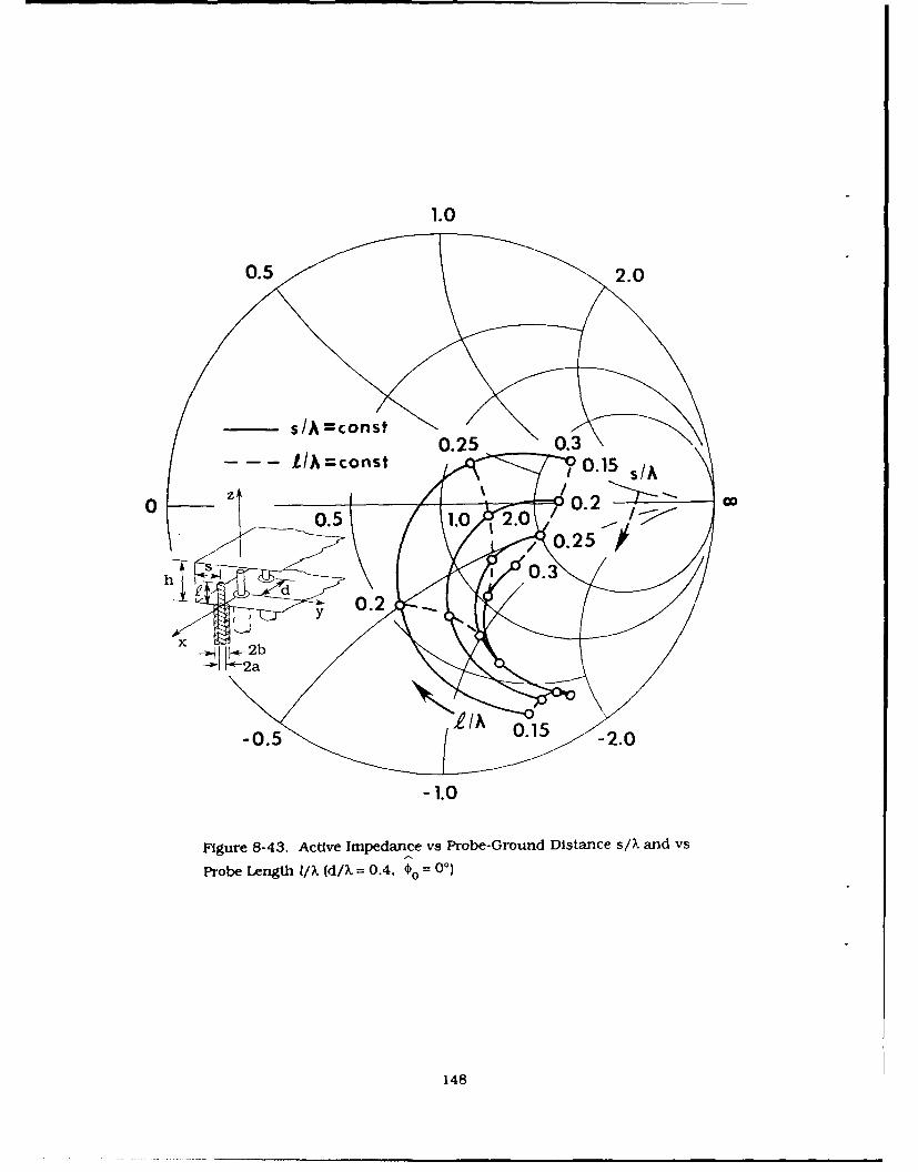
1.0

Probe ~~0 Legt 0.3/= .,* 0

const i148

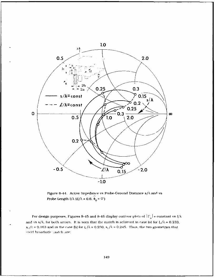
Zt 1.0

z2.

0.5

s/Alconst 01 /0.

00.1

-1.0

Figure 8-44. Active impedance vs Probe-Grotind Distance s/X and vs

Probe Length 1/k (d/k = 0.6 = 00)

For design purposes. Figures 8-45 and 8-46 display contour pints of I F constant vs l/x

and vs s/,. f-or bo0th arrays. It is seen that the match Is achieved in case (a) for 4./X = 0.233,

s,/X= 0. 163 and in the case Qb) for l/=0.250.,(X 0.245. Thus, the two geometries that

~Iitbroadside -;aatch are:

149

(a) d = 0.4 X (b) d = 0.6 X

h = 0.369 X h = 0.369 X= 0.233 X /c = 0.25 X

= 0.163 X s,= 0.245 X (8-5)

a = 0.0106 X a = 0.0106 X

b = 0.034 X b = 0.034 X

Z= = 50 Q (E, =2) Z,= 50 (e =2).

I .i 0.6

0.3 0.5

.0.4

3. , 0.3

00

0 Sc/,c 0.12 0.1zy

wx

o.1 I

0.1 0.1627 0.2 0.3 0.4

PROBE-GROUND DISTANCE, sIX

Figure 8-45. Active Reflection Coefficient - Magnitude vs Probe-Ground

Distance s/X. and vs Probe Length l/IX (d/,X = 0.4. 4o = 0°1

150

0.3~~0.4 /

I- 0. 5 -I - -.3

zW-J

W 0.2 0

Sc/c = 0.25 1I y

scc= 0.245 1I _tZ 1w2b

0.1 1 1 1 -2a

0.1 0.2 0.245 0.3 0.4

PROBE-GROUND DISTANCE, s/

Figure 8-46. Active Reflection Coefficient - Magnitude vs Probe-Ground

Distance s/k and vs Probe Length I/X (d/k = 0.6. o = 00)

We shall now vary one dimension at a time and observe the variation of active Impedance

Figures 8-47 and 8-48 exhibit the dependence of the active impedance on the probe-to-

ground distance and on probe length.

151

1.0

0.52.

0.2b

-0.5-2

S/ 0. N -1. 50.

Figur 8-47 Actie impdanc vs Pr-Grun Ditnc.15adsPrb

Legt 0/5 fo2ra a e q (-)frSeiiain.0 00) 5

-0.5 015 152

1.0

0.5

2.0

A SA

hA0.2

0 x 2)0~2a 0.52.

-1.0

Figure 8-48. Active Impedance vs Probe-Ground Distance s/k and vs Probe

Length l/X for Array (b) - see Eq. (8-5) for Specifications, % = 00)

Figure 8-49 shows the active Impedance variation at broadside scan vs parallel plateheighit h/k. It is seen from the expanded Smith chart that for hi/X variation from 0.3 to 0.45.

-J000, oI < 0.12 for both arrays. indicating that the acilve Impedance is relatively

!ttsensitive to the waveguide height.

153

OA

0.3

0.45

-0.4

d/h A 0.43-020.4d5 0.6

-~/ =. 0.3

-0.4

Figure 8-49. Active Impedance vs Parallel Plate

Height h/k for Arrays (a) and (b), (€o = 00)

The dependence of the active Impedance on the probe radius a is shown in Figure 8-50.

The radius of the outer coaxial conductor is b = 3.249 a. so that the characteristic impedance

of the coaxial feed lines always remains 50 ohms.

154

0.4

0.2

0.1

0.03

Fu0.7 08-0. c.1 men 1.3 1.4 1.5

ao Ay (a and0 1b. 0 1=32 9a o

0.1 0. .1 123

0----o d /A =0.4

-0. c - - .-o d /A =0.6

-0.3

-0.4

Figure 8-50. Active Impedance vs Probe Radius

for Arrays (a) and (b:), (b = 3.249 a, o = 0- )

It is seen that the influence of these parameters on active impedance is practically

insignificant. We conclude that the active impedance is quite sensitive to the probe length

and to the probe-to-ground distance and almost independent of the distance between the twoparallel plates and probe radius (at least with coaxial feed lines having Z, = 50 ohms).

Figure 8-51 shows the active impedance at broadside ,-s frequency for the array geometrif,

of Eq. (8-5). It is seen that the broadside bandwidth for VSW'R of 2:1 is approximately 30

percent.

155

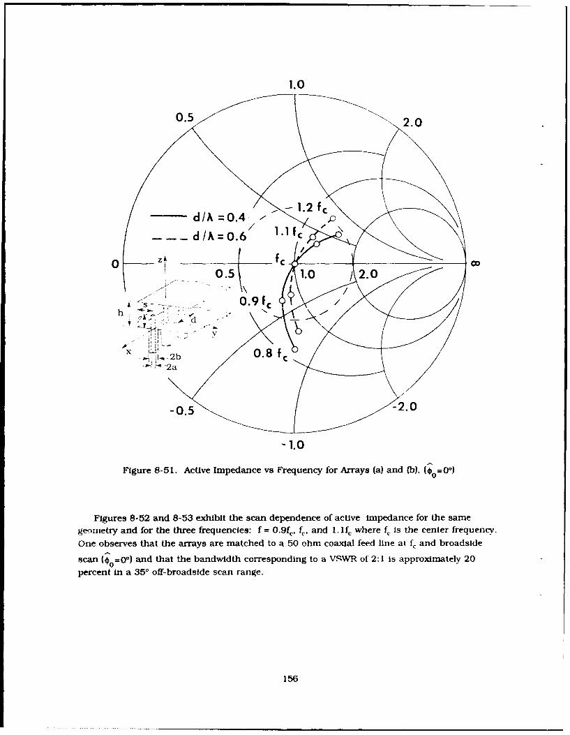
1.0

0.5

- d /A = 0 .4 . 1 . ,o- -d/A=0.6 " ,

A. ....- 0.9 0

/

:L A-. v d-

X 0.8 f_, 2b C-2a

-0.5 2 .0

-1.0

Figure 8-51. Active Impedance vs Frequency for Arrays (a) and (b). (1 =00)

Figures 8-52 and 8-53 exhibit the scan dependence of active impedance for the same

geomnetry and for the three frequencies: f = 0.9f, f,. and 1. If where f, is the center frequency.

One observes that the arrays are matched to a 50 ohm coaxial feed line at f, and broadside

scan ( n=00) and that the bandwidth corresponding to a VSqWR of 2:1 is approximately 20

percent In a 350 off-broadside scan range.

156

1.0

50.5 2.0

-0.95f

-1.00

Fiur 8 02 400eImeacev caArray~~~~~ (a) Paaetr f=/9f.f n

15720 0

1.0

00

/, fo !.*-2b C 600 fc02a 0 ° 60- 00

- 1.0

Figure 8-53. Active Impedance vs Scan forArray (b): Parameter: f = 0.9f , f,, and 1.1f,

8.4.2 PROBE CURRENT, Iz(z)

The active array probe current I,(z) has been computed using Eqs. (7-3) with V. = 1.Figures 8-54 and 8-55 show the magnitude and phase of 1, vs z/X. for the array (a) for three

probe lengths 0.15 X. 0.233 X (matched case) and 0.3 X. It Is seen that the magnitude of currentalong the probe has a basic sin k(z - 1) variation. For short probes (I < 0.15 XI. the probecurrent Is almost a linear function of z, which Is expected since sin kiz - 1) kiz - 1) when/X< 0.15.

158

30

~25E

20

0. 1

0. 1511 00

.

w

M 5

0 0.1 0.2 0.3z/Ax

Figure 8-54. Probe Current - Magnitude for Array

(a), (4bo 00): Parameter: 1P?. = 0. 15. 0.233, and 0.3

159

90

/X = 0.15

60

300

z 0 0.233

wccS

-30 -

o~~00.

-60

-90 I I0 0.1 0.2 0.3

Z/A

Figure 8-55. Probe Current - Phase for Array (a),

40 = 00); Parameter: I/. = 0.15, 0.233, and 0.3

Figures 8-56 and 8-57 exhibit the magnitude and phase, respectively, of the probe currentdistribution for array (b) for three probe lengths 0.15 X, 0.25 X (matched case) and 0.3 X. Aprobe current distribution similar to that in array (a) is found.

160

30

25

E

- 20

0. 15

0.3

0CL 5 fiX 0.15

0.0 0.1 0.2 0.3

ZA

Figure 8-56. Probe Current - Magnitude for Array

(b), o = 00); Parameter: fIX = 0. 15, 0.25. and 0.3

161

90

.. . . - - I/A -0.15

60

4)30

U 30

0.M 0.

0, ' - 0.3

-60- ..

-900 0.1 0.2 0.3

z/A

Figure 8-57. Probe Current - Phase for Array

(b), ( o = 00); Parameter: I/k = 0.15, 0.25, and 0.3

For both arrays (a) and (b), each with the three probe lengths specified above, the probe

current expansion coefficientsc' of Eq. (7-3b) are listed in Tables 8-20 to 8-25, for a single

(I = 1) and ten (I = 10) current terms in Eq. (7-3a).

162

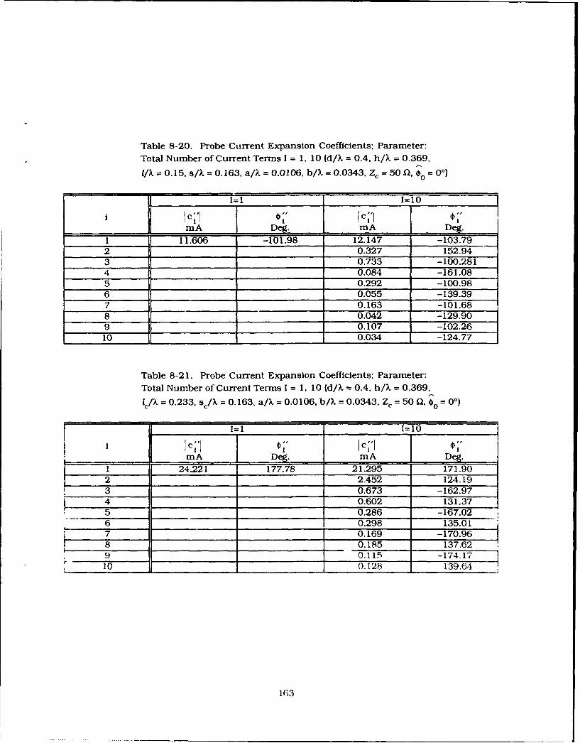
Table 8-20. Probe Current Expansion Coefficients; Parameter:

Total Number of Current Terms I = 1, 10 (d/, = 0.4. h/% = 0.369,

I/, = 0.15, s/k = 0.163, a/K = 0.0106, b/K = 0.0343, Z, = 50 Q, o 0 )

=1 I=10 1

c'I

mA Deg. mA Deg.

1 11.606 -101.98 12.147 -103.792 0.327 152.943 0.733 -100.2814 0.084 -161.085 0.292 -100.986 0.055 -139.397 0.163 -101.688 0.042 -129.909 0.107 -102.2610 0.034 -124.77

Table 8-2 1. Probe Current Expansion Coefficients; Parameter:

Total Number of Current Terms I = 1, 10 (d/X = 0.4. h/K = 0.369,

1/k = 0.233, s(/% = 0.163, a/k = 0.0106. b/X = 0.0343, Zc = 50 KI, 4o = 00)

= 1 oil, 1=10

mA Deg, mA Deg.

1 24.221 177.78 21.295 171.902 2.452 124.193 0.673 -162.97

|" 4 0.602 131.37

5 0.286 -167.026 0.298 135.017 0.169 -170.968 0.185 137.629 0.115 -174.1710 0.128 139.64

163

Table 8-22. Probe Current Expansion Coefficients; Parameter:Total Number of Current Terms I = 1, 10 {d/k = 0.4, h/k = 0.369,

1= 0.3, s/k = 0.163, a X = 0.0106, b/, = 0.0343, Zc = 50 U, = 00)

1 11=10

1c' I I;mA Deg. mA Deg.

1 10.965 137.52 9.630 139.852 2.535 95.91

3 0.268 -124.754 0.565 100.185 0.100 -135.846 1 0.268 101.777 0.052 -146.598 0.161 102.869 0.033 -157.3510 0.109 103.75

Table 8-23. Probe Current Expansion Coefficients; Parameter:Total Number of Current Terms I = 1, 10 (d/. = 0.6, h/X = 0.369,

/X = 0.15, s/X = 0.245, a/?X = 0.0106, b/, = 0.0343, Z c = 50 Q, 0 = 0 0)

1=1 1=10

n cmA De!. mA

S11.0 8 -100.31 11.454 -101.74_ 0.312 138.78

3 0.703 -98.624 0.065 -169.77

5 0.279 -99.236 - 0.044 -140.687 0.156 -99.858 0.035 -128.919 0.102 -100.3710 0.029 -122.95

164


Total Number of Current Terms I = 1, 10 (d/, = 0.6, h/, = 0.369,

/c/X = 0.25, sc/x = 0.245. a/X = 0.0106, b/X = 0.0343, Z, = 50 fl, = 00)

1=1 1=10

c; c;'mA mA Deg.

1 23.138 174.41 20.516 170.442 2.442 118.883 0.604 -159.564 0.590 126.695 0.258 -164.316 0.290 130.357 0.152 -168.778 0.179 132.959 0.103 -172.4510 0.124 134.99


Total Number of Current Terms I = 1, 10 (d/, = 0.6, h/?, = 0.369,

VIX = 0.3, s/X = 0.245, a/k = 0.0106, b/X = 0.0343, Z, = 50 U, o 00 )

1=1 1=10

Ic1 " I I c;'mA mA De.

1 13.321 144.73 11.848 146.372 2.561 98.033 0.296 -134.354 0.577 103.52

5 0.117 -145.756 0.275 105.547 0.064 -155.728 0.166 106.939 0.042 -16417910 0.112 108.04

It is Interesting to note that, since the probe current across the aperture should be

continuous, one could approximately determine the Input admittance simply from Eq. (8- 1)

that Is,

Y(8) - _z

v16

165

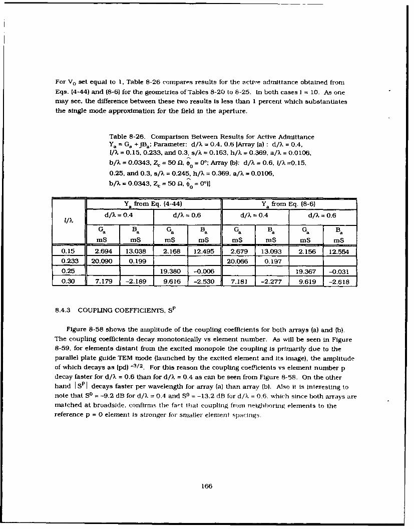
For Vo set equal to 1, Table 8-26 compares results for the active admittance obtained from

Eqs. (4-44) and (8-6) for the geometries of Tables 8-20 to 8-25. In both cases I = 10. As one

may see, the difference between these two results is less than 1 percent which substantiates

the single mode approximation for the field in the aperture.

Table 8-26. Comparison Between Results for Active AdmittanceYa =Ga +JBa; Parameter: d/X = 0.4, 0.6 lArray (a) : d/K = 0.4,I/X = 0.15, 0.233, and 0.3, s/K = 0.163, h/K = 0.369, a/K = 0.0106.

b/K= 0.0343, Z, = 50 0, 0 = 0 ° : Array (b): d/X = 0.6, I/X =0.15,

0.25, and 0.3, s/X = 0.245, h/K = 0.369, a/K = 0.0106,

b/X = 0.0343, Z, = 50 Q, ¢o = 00)]

Y, from Eq. (4-44) Ya from Eq. (8-6)

d/X = 0.4 d/k 0.6 d/X = 0.4 d/k - 0.6

G. B. G. Ba G B G BmS jmS mS mS mS mS mS mS

0.15 2.694 13.038 2.168 12.495 2.679 13.093 2.156 12.554

0.233 20.090 0.199 20.066 0.197

0.25 1 19.380 -0.006 19.367 -0.031

0.30 7.179 -2.189 1 9.616 -2.530 7.181 -2.277 9.619 -2.618

8.4.3 COUPLING COEFFICIENTS, S p

Figure 8-58 shows the amplitude of the coupling coefficients for both arrays (a) and (b).

The coupling coefficients decay monotonically vs element number. As will be seen in Figure

8-59, for elements distant from the excited monopole the coupling is primarily due to the

parallel plate guide TEM mode (launched by the excited element and its image), the amplitude

of which decays as (pd) -3/2. For this reason the coupling coefficients vs element number p

decay faster for d/K = 0.6 than for d/K = 0.4 as can be seen from Figure 8-58. On the other

hand I Sp I decays faster per wavelength for array (a) than array (b). Also it is interesting to

note that SO = -9.2 dB for d/K = 0.4 and SO = -13.2 dB for d/k = 0.6. which since both arrays are

matched at broadside, confirms the fact that coupling from neighboring elements to the

reference p = 0 element is stronger for smaller element spacings.

166

0

. -10

000. 0

~' -20 -

0z 0w -30-U- 0u.14L 0

UJ 00 -40 0

0 0 000 d/X =0.400 0 0

0 50 00000*

0-000 000

-60 o0.6

- :00a 00000

ee

-70-

-80 I0 10 20 30

ELEMENT NUMBER, p

Figure 8-58. Coupling Coefficients - Magnitude for Arrays (a) and (b)

167

180

SP I SPI e'JOP

135 & p ,- kdp

2irk 27r

90 A

0 d/X=0.445 o d/X=0.6

0L -45v=. 0

-45 -OO@ O O O O O O O.. O O. o o o o O* o* o O O

-90

-135

-180 I I0 10 20 30

ELEMENT NUMBER, p

Figure 8-59. Coupling Coefficients - Phase for AiTays (a) and (b)

Figure 8-59 exhibits the coupling coefflcent's differential phase A61, as defined in Eq. (8-4)

for two element spacings For niono)oles close to the excited el,-ment the u.oupling Is due. inaddlUon to the TEM mode. to contributions of higher, non-prip;ttij'i4g parallel platewaveguide modes. For elenients further removed, the oipliii- i- pit;narlv due to the TEM

mode.

168

8.4.4 ELEMENT PATTERN, gz(e)(()

An expression for the field element pattern gZe)(-) Is given In Eq. (6-31).

Figures 8-60 and 8-62 show the dependence of the element pattern amplitude on the

interelement spacing and frequency. In each case, the array and element geometry are

appropriate to a broadside match at center frequency f.. There are two basic differences

between the two patterns. First, broadside gain is higher for d/X, = 0.6 than for d/k. = 0.4,

which is expected since broadside gain is equal to the unit cell gain (2nd/kc} 1/2 . Second. it is

observed that while the pattern is smooth for d/k. = 0.4, for d/X c = 0.6 the element pattern

exhibits a substantial drop-off near ¢ = 420. This drop-off is caused by an end-fire grating

lobe condition (EGL) which occurs at

OEGL = Sin 1 - -I)(8) (8-7)

It is observed, however, that no element pattern null is found. This is expected, because the

Image array reduces the asymptotic decay of coupling coefficients.

169

2.0

1.1 fc

0)c

~,1.0

z

LU

0 10 20 30 40 50 60 70 80 90OBSERVATION ANGLE, -0 (Deg)

Figure 8-60. Element Pattern - Magnitude forAr-ray (a); Parameter f =0.9f,, f.,. and 1. 1 f,

170

180

0.9 fc"" 90 fc

uiCoC~1.1 Ic

z 0

I-

0.

- -90zw

-1w"S-180 I I I I I I

0 10 20 30 40 50 60 70 80 90

OBSERVATION ANGLE, " (Deg)

Figure 8-61. Element Pattern - Phase forArray (a); Parameter f = 0.9f, f., and 1.1f,

It can be seen from Figures 8-60 and 8-62 that the voltage element gain pattern does not

change significantly in a 20 percent frequency band. The pattern shape depends primarily on

d/X as already discussed while the broadside gain is governed by a factor

1(2 td/X) (i-I ra(0) 12 )) 1/2. As seen from Figure 8-62 even though the gain in the broadside

direction Is high within a 20 percent frequency band, the element has a very limited angulk:range for practical applications (up to ± 300 off-broadside at f = 1. 1f).

171

2.0

_ ~ - - -,

CD 1.1 fc .. f'1 '

-- 09f c

1.0

zC,

0 10 20 30 40 50 60 70 80 90OBSERVATION ANGLE, '(" (Deg)

Figure 8-62. Element Pattern - Magnitude for Array (b); Parameter: f = 0.9f c, fc, and 1.lIf,

For the same geometry and frequencies, Figures 8-61 and 8-63 exhibit the element pattern

phase. One observes that the phase varies only by a few degrees up to the EGL drop-off. Thus,

tihe EGL position essentially determranes the limit of usefulness of the element, both in

amplitude and phase. Since the phase reference point Is at the probe location we conclude

that the phase center location is near the probe element, This feature becomes Important In

the design of beamrforming arrays on curved surfaces.

172

I- Ni

180

0S90

Ui 0.9 f

a.

w

z -9

-

w

0 10 20 30 40 50 60 70 80 90

OBSERVATION ANGLE, $ (Deg)

Figure 8-63. Element Pattern - Phase for Array (b); Parameter: f =O.9f, . f and 1. 1if,

173

9. EXPERIMENTS

This chapter describes the experimental effort and presents measured data that strongly

support the validity of the analysis and accuracy of the computer program.To validate the theory, a 30-element linear array of coaxlally-fed monopoles in a parallel

plate wavegulde, and a one and two-half element waveguide simulator were constructed. Thearray and element construction are described. An Illustrative method of selection of optimalgeometry for element match in an array environment, as well as the dependence of importantdesign parameters on the array and element geometry is discussed. The measured data arepresented for active impedance, coupling coefficients, and element patterns. The

measurements show an excellent agreement with theoretically predicted results.

174

9.1 Array Description

The experimental array Is shown in Figures 9-1 and 9-2. The array contains 30 probe

elements in a (4 x 6 feet) parallel plate guide set-up. To simulate an infinite parallel plate

, c.on. a 5-inch pyramid of absorbing material was placed along the edges of the parallel

plates. In Figure 9-2 the top plate was removed to dsplay a section of the array. Figure 9-3

shows schematically the top and the side view of the array with relevant dimensions.

Figure 9-1. A 30-element Linear Array of Coaxially-FedMonopoles in a Parallel Plate Region. See Eq. (8-5) forspecifications

175

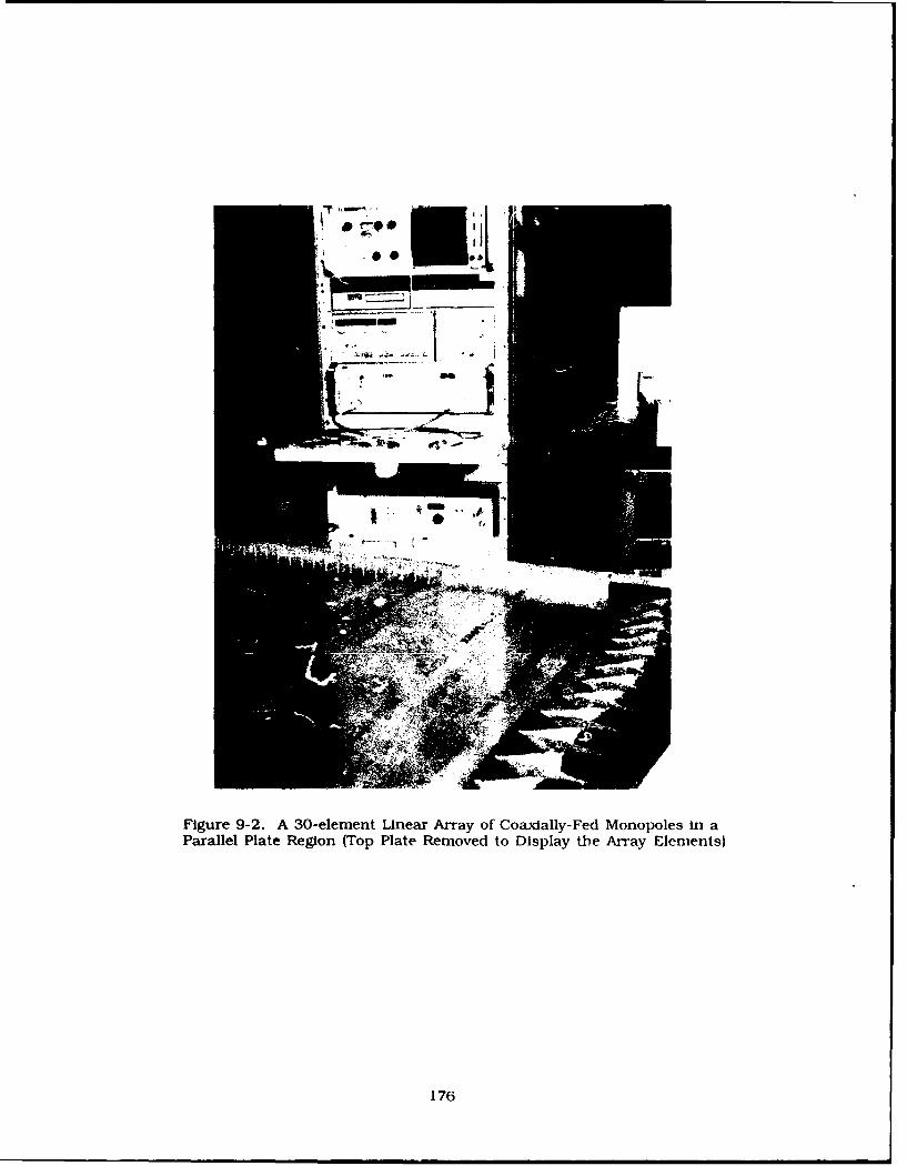
j,

Figure 9-2. A 30-element Linear Array of Coaxially-Fed Monopoles in aParallel Plate Region (Top Plate Removed to Display the Array Elements)

176

6 ft.

1~

\ 2a

4ft. @

@ d

Figure 9-3. Top and Side View of Linear Array

The linear array parameters are: , the length of coaxially-fed monopoles; h < X/2. the

parallel plate waveguide height; d. the element spacing; s, the distance between the probe

elements and the back-plane; a << X, the probe radius, while a and b are, respectively, the

inner and outer radii of the coaxial feed lines. The coaxial feed lines are filled with teflon

(er = 2) and have a characteristic impedance Z, = 50 ohms. The geometry of the array is

Identical to that of array (a) in Eq. (8-5). Specific dimensions at center frequency f. = 5.0 GHz

K = 2.360") are:

d = 0.4 Xc (0.945")

h = 0.369 kc (0.872")

= 0.233 c (0.550")

s = 0.163 'c (0.385")

a = 0.0106 X, (0.025")

i) = 0.0343 X, (0.08 "

Z= 50 Q (er =2).

The I and s were chosen to yield a broadside match at f, (See Section 8.4. 1). Parallel plate

height h = 0.872" corresponds to C-band rectangular waveguide and was chosen for easy

mulator construction.

177

9.2 Monopole Element Design

The array elements shown in Figure 9-4 are Omnl Spectra's Flange Mount Jack Receptacles

(model No. 204 CC, part No. 2052-1201-00) with a = 0.025" and b = 0.08 1". As mentioned, theelement dimensions (R and s) were determined by the requirement that the array be matched

for broadside scan (% = 00) at center frequency fc" Figure 8-45 displays a contour plot of

magnitude of the active reflection coefficient ra vs probe length 1/k c and probe to ground

distance s/%,. It Is seen that the active reflection coefficient ra40o = 0) vanishes when

1/X = 0.233, s/ = 0.163.

080 (2.4.-

.315 5 9 (12 )

050 DIA. 102 0IA, (4 PLACE .S)

Figure 9-4. Coaxial Monopole Element

For the above geometry, Figure 8-51 exhibits the frequency dependence of active impedance

at broadside scan, while Figure 8-52 exhibits active impedance dependence on scan angle *o at

f,. It is seen that the frequency bandwidth corresponding to a VSWR of 2:1 is approximately

20 percent for a scan range of 350.

9.3 Waveguide Simulator

To validate the theoretical predictions for active impedance a one and two-half element

waveguide simulator was constructed. The (single mode) simulator is shown in Figures 9-5

and 9-6. The simulator waveguide dimensions, shown in Figure 9-7, are 2d x h. that is, 1.872"

178

x 0.872", which corresponds to a standard C-band rectangular waveguide. The waveguide was

terminated in a matched load with a VSWR < 1.02 over the frequency band 4 to 6 GHz. In view

of Figure 9-8 and the relation

sin 4o = , (9-1)0 4d'

it Is seen that the device simulates scan conditions from 0= 520 off-broadside at 4.0 GHz

through = 400 at 5.0 GHz to 00 = 32 at 6.0 GHz.

Figure 9-5. A One and Two-Half Element Wavegulde Simulator

179

Figure 9-6. A One and Two-Half Element Waveguide Simulator

(Top Plate Removed to Display the Monopole Elements)

180

0.872'(0.369A)

j~0.55" (0.23A) 60

Figure 9-7. A One and Two-Half Element Wavegulde Simulator with Dimensions

d d I

hj

sin A 7

Figure 9-8. Cross Section of Waveguide SimulatorPertaining to Relation Between Frequency and Scan Angle

181

The active reflection coefficient measurements were performed with a HP-8410 Network

Analyzer. The measurement test setup is shown in Figure 9-9.

TO HP 8410 NETWORK

ANALYZCR

C-BAND WAVEGUIDE WAVEGUIDE

TERMINATION SIMULATOR

VSWR<1.02 (4.0-6.0) GHz

Figure 9-9. Active Reflection Coefficient Measurements Test Set-Up

Figure 9-10 presents a comparison of the theoretical and the measured active impedance vs

frequency. The Smith chart is normalized to 50 ohms. An excellent aR,-eement between

theory and measurement is observed across the entire band; the two results for the active

reflection coefficient differ less than 1 percent in magnitude and less than 3 degrees in phase.

182

1.0

-1.0

Figure 9-10. Acttve Impedance vs Frequency - Theory and Smulator Measurements

9.4 Coupling Coefficients

Coupling coeffcents were measured In an array of 30 elements down to -35 dB in

amplitude, which corresponds approximately to the seventh element from the excited

reference) p = 0 element. Below this level, the reflectIons from tie absorber around the edges

influenced the measured results.

Figures 9-1 1 and 9-12 present a comparison between the measured and computed values c,

coupling coefficients in amplitude and phase. respectvely. The difference between the tw-

results Is less than 03 dB !n amplitude and ees than 3 degrees in phase.

183

0

-10 IL

S -T zt

-20 -0 V d

0'. S0(j -0 ~ 4 I~j2b- 30

zwt 0006. -40

U-0U(-) -50 --

oTHEORY 0

-60 .0 MEASURED ELEMENTS (0-7)0 -600 DIFFERENCE IN AMPLITUDE < 0.3 dB

-70

-80

0 10 20 30

ELEMENT NUMBER, p

Figure 9-11. Theoretical and Experimental Amplitude of Coupling Coefficients

184

180

135

SP = I sPI e'JP90

Ap O= - kdp

45 k 27

0

0.

<1 -45 O O 0 O O O O O 0 0 0 0 0 0 0

-0 L

.90 THEORY

0 MEASURED ELEMENTS (0-7)-135 DIFFERENCE IN PHASE < 30

-180 I I

0 10 20 30

ELEMENT NUMBER, p

Figure 9-12. Theoretical and Experimental Phase of Coupling Coefficients

9.5 Element Pattern

A linear array of 11 monopoles in a parallel plate region was used to measure the elementpatterns on a 2000-foot antenna range. A photo of the antenna on the test posltioner is shownIn Figure 9-13. The test fixture has a semi-circular E-plane flare as shown in Figure 9-14, toimpedance match the wavegulde to free space. The axis of rotation was at the center elementprobe location. This element was connected to a 20/20 Scientific Atlanta Antenna Analyzer:other array elements were match-terminated with 50 ohm coaxial loads.

185

I"

Figure 9-13. Eleven-Element Linear Array on Far-Field Range

186

11 ELEMENT ARRAY

t E

TRANSMITTER

Figure 9-14. Test Fixture for Element Pattern Measurements

Figures 9-15 and 9-16 show the amplitude and phase of the element pattern vs observation

angle 0 for the following geometry: h/, = 0.3, d/, = 0.72, I/X = 0.22, a X = 0.019, b/X = 0.062 at

f = 3.0 GHz. The amplitude pattern is normalized to the unit cell voltage gain (21d/X)1/ 2 . It is

seen that the amplitude and phase curves are approximately constant up to = 25- off-

broadside. The amplitude pattern exhibits a substantial drop-off near = 250 while the phase

pattern begins to vary rapidly with the observation angle. The sudden change of amplitude

and phase patterns is caused by an end-fire grating lobe effect as explained in Section 8.4.4

which for inter-element spacing d/X = 0.72 appears at 25' array scan off-broadside.

187

0

-5

z -10-

z - MEASURED2-15- .... CALCULATEDILn-JIl

-20 . I0 10 20 30 40 50 60 70 80 90

OBSERVATION ANGLE, $ (Deg)

Figure 9-15. Theoretical and Experimental Element Pattern Amplitude

90

d0 45- ,0

w

5-.

I-< --MEASURED.-- 45 ... ~CALCULATED

z

0J

:Z0

I-

,.w

S-90I0 10 20 30 40 50 60 70 80 90

OBSERVATION ANGLE, Q (Deg)

Figure 9-16. Theoretical and Experimental Element Pattern Phase

188

Since the phase is referenced to the center element, Figure 9-16 also indicates that in the

region 00 < < 25' the "phase center" coincides with the probe location. The ripple in both

curves is caused by array edge effects.The dashed curves In Figures 9-15 and 9-16 represent the theoretical element patterns of

the monopole element In an infinite array environment. Good agreement between measureIand theoretical results is observed.

10. CONCLUSIONS

An accurate analysis is presented of scan characteristics of an infinite linear array ofcoaxially-fed thin monopole elements in front of a perfectly conducting backplane in aparallel plate wavegulde. Expressions for the active admittance, element patterne andcoupling coefficients are given. The relevant expressions can be also applied to arrays in aninfinite wavegulde region as well as to a single monopole radiating into an infinite or semi-infinite parallel plate region. The numerical results lead to the following conclusions:

(1) A design method for a matched array element without inclusion of an extra matchingnetwork has been established. It is shown that for a given spacing, scan angle and frequency,the element can be perfectly matched by an appropriate choice of a pair of values for L /X ands,/X: at least when Z. = 50 QI. It is found that the active admittance is relatively insensitive to

the parallel plate separation and to the probe radius (as long as characteristic impedance ofthe coaxial feed line is 50 ohms). The active impedance exhibits a significant dependence onmonopole length (1/k) and on Its distance (s/X) to a conducting ground.

(2) With such element design, the frequency bandwidth corresponding to a VSWR of 2:1 isapproximately 20 percent for a 350 off-broadside scan range.

(3) The element gain and phase patterns are predictable. The amplitude and phase curveq

are approximately constant up to the angle OEGL off-broadside (the end-fire grating lobe

condition). The amplitude pattern exhibits a substantial drop-off near EGL while the phase

pattern begins to vary rapidly. Thus the EGL position essentially determines the useful rarge

of the element.(4) The dipole phase center is located near the element. This information is Important in

design of microwave feed-through lenses and conformal arrays because it defines the effectiveradius of curvature of the array surface.

(51 Close to the excited element the coupling is due to the TEM parallel plate guide mode. .well as to contributions of non-propagating parallel plate wave5ulde modes. For elementsfurther removed, the coupling is primarily due to the TEM mode. the amplitude of whichdecays as (pd)-2 / 3 for an array backed by a conducting ground.

(6) Simplicity, low cost, polarization puilty, reasonably wide bandwidth, and relativelligh power handling capability make the coaxial monopole a practical element tor arra.-parallel plate regions.

189

(7) The close agreement of the experimental and theoretical results for active impedance,

coupling coefficients, and element patterns strongly supports the validity of the analysis, and

furnishes a firm basis for the matched element design method that was developed.

190

References

1. Tomasic. B. and Hessel, A. (1982) Linear phased array of coaxially-fed monopole elementsin a parallel plate guide, IEEE/AP-S Symposium Digest. 144, Albuquerque,New Mexico.

2. Tomasic, B. and Hessel, A. (1985) Linear phased array of coaxially-fed monopole elementsin a parallel plate waveguide - experiment, IEEE/AP-S Symposium Digest, 23,Vancouver, Canada.

3. Tomaslc, B. and Hessel, A. (1985) Arrays of coaxially-fed monopole elements in a parallelplate waveguide, Phased Arrays 1985 Symposium - Proceedings, RADC-TR-85-171,223-250, ADA16931.

4. Williamson, A.G. and Otto, D.V. (-973) Coaxially-fed hollow cylindrical monopole in arectangular wavegulde, Electron. Lett., 9, (No.10):218-220.

5. Williamson, A.G. (1985) Radial line/coaxial line Junctions: Analysis and equivalentcircuits, Int. J. Electronics, 58, (No. 1):91-104.

6. Hildebrand . F. (1962) Advanced Calculus for Applications, Prentice Hall, Inc., EnglewoodCliffs, New Jersey.

7. Williamson, A.G. and Otto, D.V. (1973) Coaxially-fed hollow cylindrical monopole in arectangular wavegulde, Electron. Lett., 9(No. 10):218.

8. Papoulls, A. (1977) Signal Analysis, McGraw-Hill, New York.

9 Infeld, L. at al (1974) On some series of Bessel functions. J. Math. and Phys.. 26:22.

10. Abramowltz, M. and Stegun, [.A. (1964) Handbook of Mathematical Functions, UnitedStates Department of Commerce, National Bureau of Standards, Applied Mathematics,55.

11. Lee, S.W., Jones. W.R. and Campbell, J.J. (1970) Convergence of numerical solution of iristype discontinuity problems. Antennas and Propagation Symposium Digest. Columbus,Ohio.

191

12. Conte, S.D. and de Boor, Carl (1972) Elementary Numerical Analysis, McGraw-Hill, NewYork.

13. Felsen, L.B. and Marcuvitz, N. (1973) Radiation and Scattering of Waves, Prentice Hall,Inc., Englewood Cliffs, New Jersey.

14. Gradshteyn. I.S. and I.M. Ryzhik, I.M. (1965) Table of Integrals, Series, and Products.Academic Press Inc., New York.

192

Appendix A

Field Representation in Regions with Piecewise Constant Properties

Al DERIVATION OF THE TIME-HARMONIC FIELD FROM SCALAR POTENTIALS

As described In Reference 13, the electromagnetic fields excited by time-harmonic electricpoint currents J(r,t) = JO 8(r-r') e Jot and magnetic point currents M(r,t) = MO 8(r-r) eiJt may berepresented at r # r' as:

E(r.r') = V x V x zo rl'(rr') -Jo* V x z0 Hl"(r.r') (A- la)

H(r.r') =JoE V X z0 lr'(rr') + V x V x z. r"(rr') (A-lb)

13 Felsen, L. B. and Marcuvitz, N. (1973) Radiation and Scattering of Waves, Prentice Hall,Inc.. Englewood Cliffs, New Jersey.

193

where the E (prime) and H (double prime) mode Hertz potentials n' and n", respectively, arerelated to the scalar potential functions 8' and 8" via

H'(rr')= __I_ Ov'xV'xz O 8'(rr')- M*V'xz 0 S'(r,r')JCOE (A- Ilc)

l"(r.r') = J0oV × z0 8"(rr') + 1__ M0 V' x 1V' x z S"(r,r').JCO R (A- I d)

The longitudinal electric current element Jo= zo JO M O = 0, contributes only to l'(rr'),

thereby exciting E-modes only, and a longitudinal magnetic current M 0 = zo M 0, J 0 = 0.

generates only H-modes, whereas both mode types are excited by a transversely directedsource

of either electric or magnetic current. If E(r,r') and H(r,r') satisfy the Maxwell field equations

for point current excitation, then 8'(r,r') and 8"(r,r') satisfy the differential equation

(V2 + k2) Vt S'(r,r') = 8(r-r') (A-2a)

(V2 + V2 8"(r,r') = 8(r-r'), k2 = 2 (A-2b)

subject to appropriate boundary conditions. By defining

-V2 S'(rr') = G'(rr') (A-3a)t

-V 2 8(rr') = G"(rr') (A-3b)t

one may relate S' and S" to the corresponding Green's functions G' and G" of the scalar wave

equations by

(V2 + k2) G'(r,r') = -8(r-r') (A-3c)

194

(V2 + k2 ) G"(r.r') = -((r-r'). (A-3d)

Since an arbitrarily oriented source may be decomposed into a transverse and longitudinal

part, it is useful to list the corresponding reduction of (A-ic) and (A-id) for these separate

cases. When the source is transverse d = z ,

l'(r,r') = I- Jt 0 a M t 0x z o ) t tr,r') (A-4a}

oo(rr') =__+_C) V'S"(r,r') (A-4b)" (r 0 = j0O1 t × a

whereas for a longitudinal source J= M= ).

0

rl'(r.r') = G r (A-4c)J(O C

rz(r~r') =- G"(r,r'). (A-4d)

From transmission line analysis along the z axis, with eigenfunctions evaluated in the cross

section transverse to z, one has the following solutions of Eqs. (A-2) and (A-3) in terms of a

modal expansion:

s'(r.r') = 0 %(p) 4 ;(p') Y(Z k' * 0 (A- 5a)J¢.oC k k 2 Y(ZZ) i A-5a)

tt

195

S"'(r.r') = kL. "(p) 0"Z( z0AJok I 2 ftzz''k u (A-5b)

or,

j'(rr') 0(p) 0 ;p') Y (zz') (A-5cJCDeI

G"(r.r') = __. 'i(P) 'Po') Z' (z,z'). (A-5d)

It Is recalled that O,(p) and 'P,(p) are scalar eigenfuctions that have been listed in Reference 13

for a variety of cross sections. The Y'(zz and Z 7(zz') are, respectively, the E-mode current

excited by a unit voltage generator and the H-mode voltage excited by a unit current generator,

and they are related to the one-dimensional E-and H-mode Green's functions by

Y;(zz') =JWE g,(z,z') (A-6a)

Z (z,z') -Jo)A g"(z,z') (A-6b)

where g zi(zZ') and g'"(z,zl satisfy the equation

(d;?+ N) g.i(zz') = -8(z--z') (A-6c

with

2 2 2=k k (A-6d)

subject to appropriate boundary conditions at the endpoints of the z domain.

196

A2 MODAL REPRESENTATION FOR UNBOUNDED CROSS SECTIONS

Because there are no transverse boundaries, the eigenvalue problems for the E- and H-

modes are identical so that 4', = P,. and the distinction between the E- and H-mode Green's

fuction resides solely in their longitudinal dependence. For the circular waveguide

description of G(rr') (with 4 denoting kt).

2nrr' M-- 2- -m ¥f0 J4 J P ) JM(R0' gzl(Z Z': 1c) d " (A-7)

It will be useful to employ a representation involving a range of integration in 4 from - 00 to

instead of Eq. (A-7). Provided that g ,,(zz') is an even fuction of 4, a requirement satisfied by

the longitudinal Green's functions to be encountered subsequently, the desired representation

may be derived as follows. Upon introducing

n -[Hn()(4p) + 2A-8)

where H()(Ep) and H2)( p) are the Hankel function of the first and second kind of order m

and argument p. One may write Eq. (A-7) as

G(rr')- e--m() (Ii + 12) (A-9a)

where

1 = "(P) J,,( P') d7 (A-9b)

197

12 =2 f H((4p) J (4p') d 4. (A-90)

If the range of is to be extended to 4 = - c, the = 0 branch-point singularity arising from the

presence of the Hankel function [and also of the Bessel function in (A-7)), must be accountedfor In the Integrands of I1 and 12, since m Is not an Integer. To assure single-valuedness of the

intregrands when continued into the complex E plane, we introduce a branch cut along the

negative real axis (see Figure A-1). The following parametric relations then provide the

means for mapping into - (0 < <):

Jm(xeJX) = ej n I Jm(x) (A- 1Oa)

H2')(xeJx) = e ra H(2)(X). (A- 1Ob)

Suppose we introduce the change of variable 4 = e-i' In the ntegrand of I in Eq. (A-9bJ.

Then,

(A-1 la)

d = ej" d (A- lIb)

and

-jig

2 Je 4e .im( pe) d-

or,

198

0

I, =i '(p J. W (A-Ild)

where Eq. (A-ld) follows from Eq. (A-11c) and the use of Eq. (A-10). Thus, I1 + 12 may be

written as

1 +1 4, H((p) J.( p) d= ~H~()p') J( p) d .1 + 2 2 f~ell m me -jn m (A-12)

im~

BRANCH CUT

* WV TWY V ~V V V Vy V V V V

v ReC2

Figure A-I. Integration Path in the Complex -Plane

The contour of integration extends along the bottom edge of the branch cut and the positivereal axis as is shown in Figure A-1. The alternative expression with p and p' interchanged.given by the second integral in Eq. (A- 12). is deduced by representing Jm(4p') in Eq. (A-7) in

terms of the Hankel function contribution in Eq. (A-8), and proceeding as above. The integralrepresentations in Eq. (A-12) permit deformation of the contour of integration into the

complex 4-plane. To show this, we examine the asymptotic behavior of the Bessel and Hankeifunctions for large values of their argument:

199

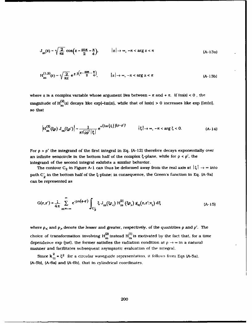
(.2) ) -2 e- (zJ - i-- ), IzI- - , - x < argze4 (A- 13b)

where z Is a complex variable whose argument lies between - 1C and + n. If Imiz) < 0, the

magnitude of H (2){z decays like exp[-lm(z)I, while that of Imz) > 0 increases like exp JimjzI],m

so that

1H () JM(W) 1 e+(Imlt l )( p-P') I41-+ -, -n < arg , < 0. (A- 14)

For p > p' the integrand of the first integral in Eq. (A-12) therefore decays exponentially over

an infinite semicircle in the bottom half of the complex t-plane, while for p < p', the

integrand of the second integral exhibits a similar behavior.The contour C2 in Figure A- 1 can thus be deformed away from the real axis at I I - o into

path C' in the bottom half of the -plane; in consequence, the Green's function in Eq. (A-9a)

can be represented as

G(r,r') -Jm() m(<) H 2)

4n .P-1)H. p>)g.,(~z',K,)d A- 15)

where p< and p> denote the lesser and greater, respectively, of the quantities p and p'. The

choice of transformation involving H(2 ) Instead H ( })Is motivated by the fact that, for a time

dependence exp U(o)t). the former satisfies the radiation condition at p -4 - in a natural

manner and facilitates subsequent asymptotic evaluation of the integral.2

Since kt2 = 2 for a circular waveguide representation. It follows from Eqs (A-5a),

(A-5b), (A-6a) and (A-6b), that in cylindrical coordinates.

200

where g ,fz.z': Ic) depends on k through the longitudinal propagation constant

201

Appendix B

Magnetic Ring Source In An Infinite ParallelPlate Waveguide - Radial Mode Representation

B 1 RADIAL TRANSMISSION LINE REPRESENTATION

In this Appendix we derive expressions for the fields in the parallel plate region due to a

magnetic ring source of width (b-a) by an approach in which the propagation direction Is

assumed to be radial. The problem is simplified by first considering magnetic ring source

excitation with M(p'.z') = 0o 5(p - p') 8(z - z'). (z'=O), and then obtaining the total response by use

of the superposition theorem.

Since the magnetic source is transverse (to p) with a/Dlb' = 0, only E-modes with respect to p

are excited. Field components transverse to p can be expressed in the form

E,(p.,.z) = Z V'(p)e (B-la)n=0

203

n= 0n 1

where the E-mode transverse vector elgenfunctions e' and h - areZn +

ez(O,._ cos nz (B-Ic)-/2- h h

h (p,z)- 1 _ 1 cosnt z (B- id)

h' vP- hp h

with

1, n=O2, nB-!e1

The e' and possess the following orthonormality properties over the cross-sectionalZn

domain S

f e' xh' " Po dS= 8n, dS=pdodz.f(B-2)

The asterisk denotes the complex conjugate, and the Kronecker delta is:

8 = 0. m * n; 8 = 1. In Eqs. (B-la) and (B-lb) the total modal voltage and current are

V'n(p) = V(pp') dp' (B-3a)

204

I I (P) i,(p.p') dp' (-bn f (B-3b}

where Vn(p.p') and In(p,p') are voltage and current at p due to point sources v'(P') and I n(p') at

p'. Since M(p'.z') Is transverse (to p). the magnetic current ring source can be represented by a

point voltage generator v'n(p') on an equivalent radial transmission line at p', where

v '(p') = ff M(pp')" h'* (p'.0'.z') dS

source

2n 0 MHO) E cos d "z' p'd= -Mf2n/E" n (B-4)

The radial transmission-line equations that apply to the indicated point-source excitation are

-- v (p.p') =JK Z' i " (pp')+ v '(p')dp nnp (B-Sa)

dp (PP)Jn.dl pv n(pnp') (B-5b)

where

z'=- 1 Inn yP WE 0 (B-5c)

i - n-InI o. (B-5d)

To determine V n(p'p') and I n(p.p') we first determine the amplitude of the voltage and cunent

at the generator terminals p' and p' . The determination of voltages V n(pp') and currents

205

'(p.p') at any point p on a transmission line with constants icn and Zn then follows from Eq.(B5n

To that end. we consider the network problem shown in Figure B-i1. where Z (p') and Z(p')

are the impedances seen looking to the left and to the right, respectively, from the generator

terminals.

ZWp) Zipi

Figure B-i. Network Representation for Voltage Point-SourceExcited Radial Transmission Une

The voltage V'(P) satisfies Bessel's differential equation

s' p d ) + 1v n(p 0 (B-Ga)

and for p < p' the solution can be written in the form

V'(p)=JKC Z' J p) p < (B-6b)

Substituiting Eq. (B-Gb) into Eq. (B-5a),

n' (P)= KPJ I "P). - B-7)

Using Eqs. (B-Gb) and (B-7)

206

zj (P') . . .. j - () z 7(p' p' (' p')(B-8)

Sinilarly. for p > p', the solution of (1-6a) is

(2)V(p) =J K Z' Ho (icP) p>p' (B-9a)

and after substitution into Eq. (B-5a),

from which we get

-. Vn( P') Zn I(cp)Z(p<)= In(+' ( (B-9c)In(~) P' H I (Kp'

By conventional network analysis it Is seen that

Vi( p,) -v (p) (P (B- lOa)n Z(P')

pp') v ',(p') :. (B-10b)Z(p')

."J'0re

207

Z(p') = z(p') + , (p'). (-10c)

Substitution of Eqs. (B-8) and B-9c) into Eq. (B-10) yields

VPP) K NP (2)V 2n.p) -J 2 v'(p') H0 (icp') J(icp ') (B-a)

V2'(p p') =-J K HV (n p') (B- 1lb)

and

, (2) (13- 1Ic)i ipi

2 J QnP)HI (IC1nP')

where we have used the Wronskian relation

W[Jo((np,). (2)( np,)] =j (2) , (2) , 2w[J0 (cp)) H (Kc~ JIPp~H ') - J (ICP') H (1c p')j(B1n n I n 1n/ nJ OnJ 1B-lid)

In view of (B-6b) and (B-9a) the modal voltage on the radial transmission line at p due to

the point source at p' follows from Eqs. (B-I la) and (B-i1 b), that is.

1 (2)V ( ,,P" ;(') oP ,(P, I ,K n ') -o (,.P,o) P > P'

2= - v( {Jo(c.)H 0 (c). , <' (B-12a)

or upon substitution of Eq. (B-4) forv '(p')

208

V'(pp') = -J 0 en1 (2) (B-12b)n2 IbI h 1J0 c 1 nK) ~

a

Equation (B-12b) can be briefly checked by noting that the Identity

V$(,P') + v'(P')- V'(p-.P')no (B-13)

must be satisfied. Substituting Eqs. (B-1 la). (B-1 lb) and (B-4) Into Eq. (B-13) one finds that

indeed Eq. (B-13) holds.

The modal voltage due to the magnetic ring source of width (b-a) can now be obtained from

Eq. (B-3a) where the integration over p' extends over the source region. Thus,

v,(p) =-jKn 2nV ,nn n 0 Vnha

bHo'2 (K P) I J,(icp')dp' p-b

H 2 (Kp) f j 1 (,cP') d p' + Jo(x.p) J H(x .p') d p', a5 p: b

Jo(Qcp) 1 b -H,)(K.pt) d p' . -<a

-I2nb h 1J(K"p) I-I° 2(Kb) -H0 2(' P) J0 (K a). a<_p<b (B-14a&a

SJo(K, p) p a

where

209

l~~~ (K A in p bll lll IIl

in = J0{vnb) - Jo(cna) (B- 14b)

ifn = H 2 )(K nb) -H 2 c(na). (B- 14c)

Substituting Eq. (B-14) into Eq. (B-la) with ezn defined in Eq. (B-Ic), we see that the z-

component of the electric field due to the magnetic current ring source at z = 0 in an infinite

parallel plate waveguide is

Ez(r) = Vn(p) e Zn(O'z)

H0 (Knp) Inpb

-J 2ln~ X cos 1~- J (2~) - (2)V0 E Co nz JO(Kp)Ho' (2) _b o H (p) Jo( a). a : p : b. (B-15)-2hIn h n=o n n

aJ 0 (Knp) ' p 5 a

The magnetic field I-(r) can be obtained from Eq. (B-lb) using Eqs. (B-5a) and (B-12) as

demonstrated below. From Eq. (B-5a) at p * p',

I (pp") = - P ----- v4 Vn(p, p,). ( -6n -c Z' dp n (B16)

n it

Substitution of Eq. (B- 12) into Eq. (B-16) yields

( (2)Kp -V'2rV TE I J,(",,p() 2, (Kp). p > P

1 '(p.p') 0Z 2I a J (KP) H (2 Kp'). p <P (B-17)

Consequently, using Eq. (B-3b) one has

210

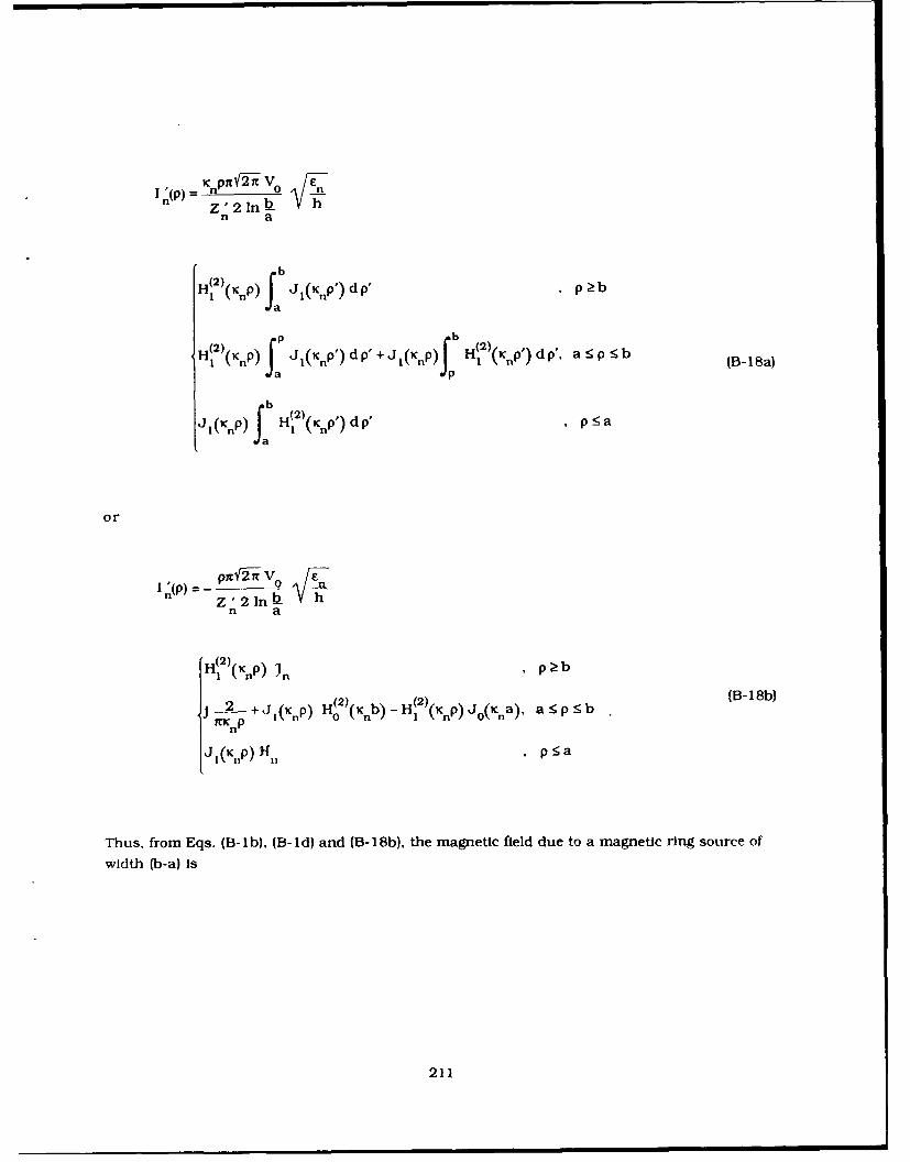
= K pnO-ln V0Z'2In

b - hn a

b

H )(K) a J( ') dP' p 2b

H )(2 p) 1(K p')dp'+JQc,(P) H (2 (,Cp') dp', a <pb lB- ap)

b

JI(KnP) a H12) (Kp') dp' p 5a

or

Ip' pf -piV 0 FE

n a

Hd2(p) ( , p_<b

+ ~ (2) (2) (13- 18b)2 + 1 (K P) H0' (IC nb) -H, (1C.p)J 0 (K na), a5p! b

Xnp

J I K.p) 1f11 p:5a

Thus, from Eqs. (B-Ib), (B-Id) and (B-18b), the magnetic field due to a magnetic ring source of

width (b-a) is

211

H (pz)n=I10 V -Co 1 z

H, (Kp n , p?<a2m +J 1 Q n 0 (nc) IH (1 np)JQ~) n~ (B- 19a)

where

K=-

2h In b_ (B- 19b)a

B2 RADIAL MAGNETIC GREEN'S FUNCTION REPRESENTATION

The expressions for the electromagnetic field in an infinite parallel plate region due to an

annular aperture driven by a coaxial transmission line are derived in this section by analternative method using a magnetic Green's function G(m).

An open-ended aperture ot a coaxial line of inner and outer radii a and b, respectively, is

considered to be located on the bottom plate of the perfectly conducting infinite parallel platewaveguide of height h as shown in Figure B-2. A cylindrical coordinate system (p,,z) is chosen

with z along the axis of rotational symmetry of the annular aperture. The aperture electric

field is assumed to be that of the TEM transmission line mode

VE(p,z=O) = po v a psb

ln b. (B-20)

where V0 is the modal voltage at the aperture.

212

x,

Figure B-2. Coaxlly Driven Annular Aperture In an Infinite ParallelPlate Waveguide

Using the equivalence principle, the problem of Figure B-2 becomes that of a magnetic ring

source in the infinite parallel plate waveguide as shown in Figure B-3. where the magnetic

current density is

M(p,z;t) = P M,(p' z) e Jt; a <! b (B-21 a

with

VM (P.z) = ---- 8(z).

pIn - (B-21b)a

213

x

Figure B-3. Annular Magnetic Current Ring Source in an InfiniteParallel Plate Waveguide

To determine the P - ' in the parallel plate region due to the magnetic current density of

Eq. (B-21a) it is conv-uent to formulate the problem in terms of the single component of the

magnetic field H ,. We readily find that H* satisfies the differential equation

2

[L_ - (pH,)] + k2H +I = JWE 0 M, (B-22aap pa z2

which follows from Maxwell's equations

V x E = -J (o go H - M (B-22b)

VxH=Jwo0 E (B-22c)

with a/a=0. The condition a/a=O is due to absence of angular variation of M * and the

rotational symmetry of the structure.

The associated electric field components are

214

E-=- IB-23a)

" Jo(% az

E =1 - (pH*) (B-23b)

with

E HP z = . (B-23c)

The solution of Eq. (B-22a) can be written in terms of a magnetic Green's function as

bH,(p,z) = -J fop'a M,(p',z') G(m)(p.z;p'.z') dp'. (B-24)

The Green's function Gm) which represents the magnetic field due to a unit magnetic current

loop (shown in Figure B-4) satisfies the differential equation

a (pG m) ) + k2G(m ) + 2 -8(p-p') 8(z-z'). (B-25)ap pap2

215

z

x

Figure B-4. Unit Annular Magnetic Current Loop in an InfiniteParallel Plate Waveguide

An appropriate solution to Eq. (B-25) can be written in the form

Gm)(p'z ') = gn(P'P') cos nR z f(z'). (B-26)n=O h

Substituting Eq. (B-26) into Eq. (B-25) and then multiplying both sides of Eq. (B-25) bycos (nnz/h. and integrating from z=O to h, where we use the orthogonality property of theelgenfunctions and the integral property of the delta function, we obtain

(z) = cos (B-27aJ

where

1, n=0

En =-- 1 2, n _ I (B-27b)

216

Substitution of Eq. (B-26) Into Eq. (B-25). and then Eq. (B-25) into Eq. (B-24) yields thediffe-ential equation for the radial Green's function g n:

1 -i A+ K 2 _I' ) g (P'P') =- (P-P')(Pdp dp n 2)l (B-28)

The solution for gn' which satisfies the homogeneous differential equation corresponding to

Eq. (B-28) is

=nP- AJ2KA p, (B-29)[BHJ (InCA, p>P

which ensures finiteness of g, at p=O and decay of g n as p --4 C. The JI(inp) and H (n(Kp)

denote Bessel functions of the first kind and Hankel functions of the second kind, both of first

order. To determine the coefficients A and B. we use

gn(p'+A.p') = gn(p-A-p'), A --4 0 (B-30a)

dg(Pp + =-1, a-- 0 (B-30b)

dp OA

which gives a system of two simultaneous algebraic equations

H2) A B' IP (B-30)ij (.' - H 2' (K.P') B K

-H 1p' I'~ n

Solving Eq. (B-30c) we find

217

A -(B-31a)2 n

B=- L'- J1 (Inp') (B-31b)

where we used the relation for the Wronskian

W{J, (x), H )(x)} -. (B-31c)v 1Cx

Consequently,

gn(P,)- J I -- np.J( H (2) (B-32)g~p~') 2 ~ (C< 1 ('%P>)

Substituting Eqs. (B-26) and (B-32) Into Eq. (B-25), the Green's function G (m ) is

(m)(p ,zp' ) = -c, -J 2X J Kp) H2(Kp) cos -- z cos n ' (B-33)

2h n=0 (K P-<, h h

Using this result in Eq. (B-24) we can now determine the HO due to a magnetic current

distribution [Eq. (B-2 lb)]. After integration we get

218

P o 2 h ln b -n= 0 D

H,2 (K np) [Jo(K nb)-Jo(na) p a)b

(2) (2)j ---- +,j Q) H0 (r. b) - H1, (r-p J0 ca)-. a p! b (-XrK P N n o'n(-4

which upon substitution into Eqs. (B-23a) and (B-23b) gives the field components EP. E,.

219

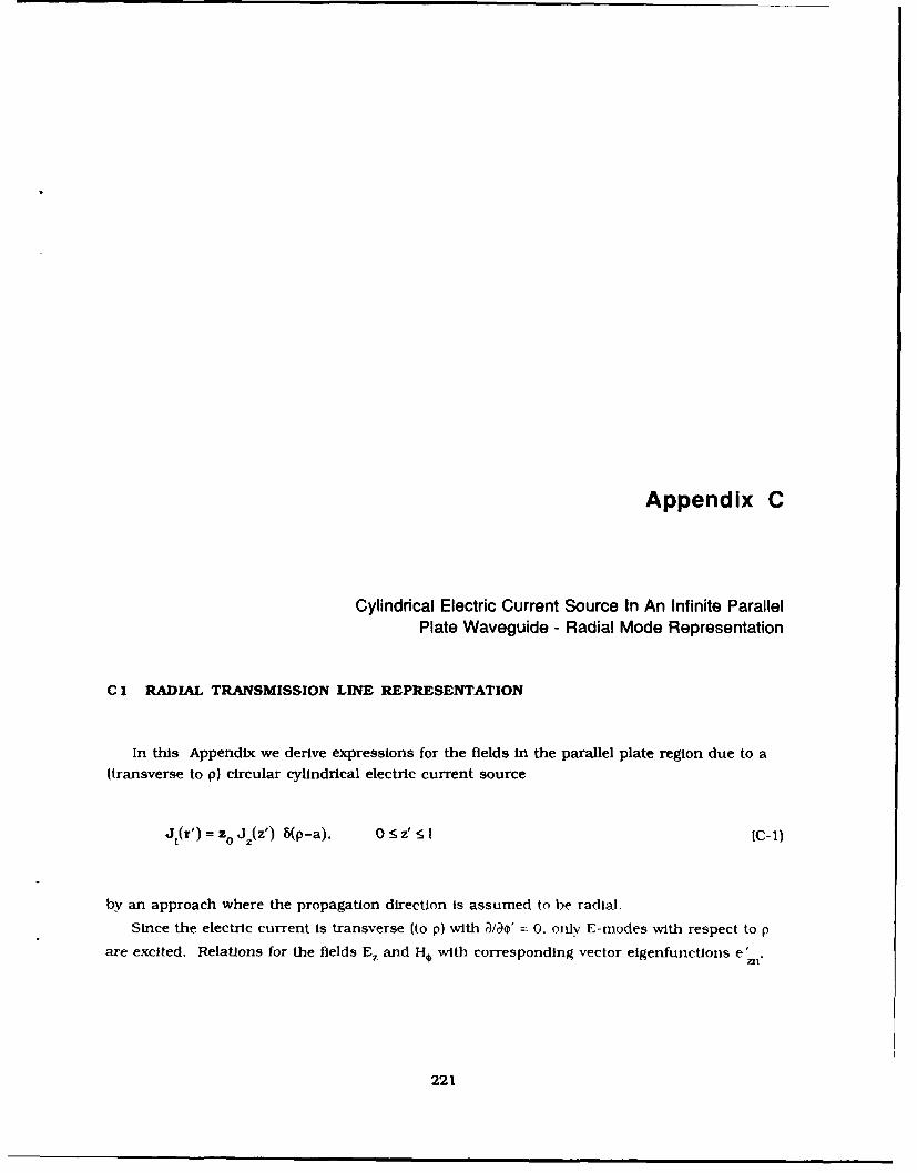
Appendix C

Cylindrical Electric Current Source In An Infinite ParallelPlate Waveguide - Radial Mode Representation

C 1 RADIAL TRANSMISSION LINE REPRESENTATION

In this Appendix we derive expressions for the fields in the parallel plate region due to a

(transverse to p) circular cylindrical electric current source

Jt(r') = z 0 Jz(z') 6(p-a), 0 < z' < I (C-1)

by an approach where the propagation direction is assumed to be radial.

Since the electric current is transverse (to p) with a/ai' = 0. only E-modes with respect to p

are excited. Relations for the fields E z and H, with corresponding vector elgenfunctions e zn'

221

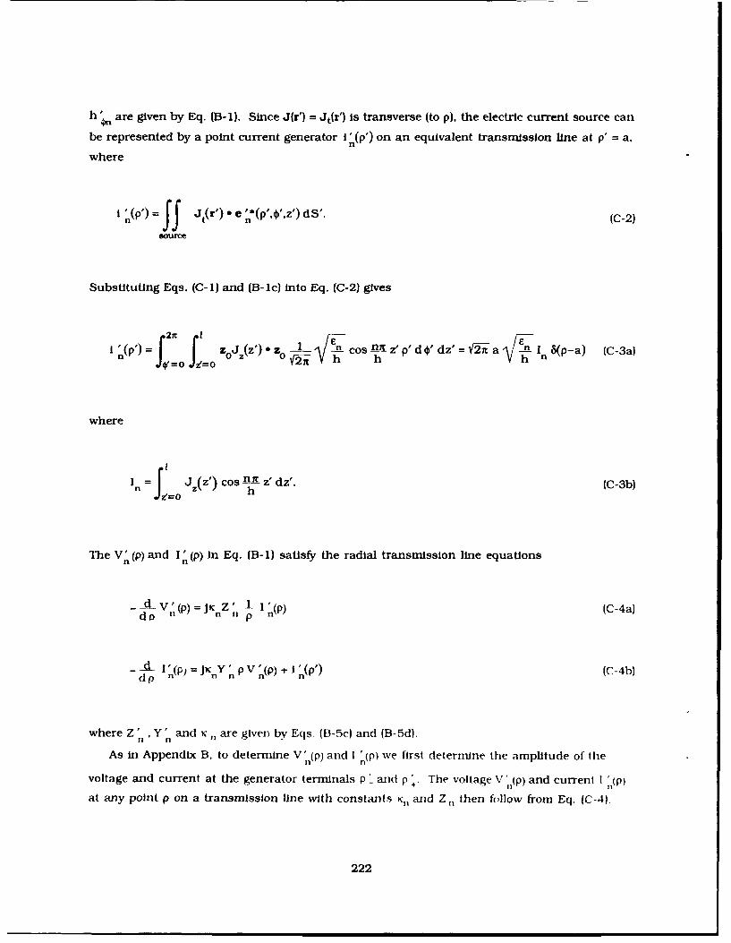
h ' are given by Eq. (B-i). Since J(r') = Jt(r') is transverse (to p). the electric current source can

be represented by a point current generator i (p') on an equivalent transmission line at p' = a,n

where

n = f t(r') . e n (p', ,z') dS(. C-2)

souc

Substituting Eqs. (C-i) and (B-ic) into Eq. (C-2) gives

21t I

(p') = f f zoz (z')* z cos n1 z" p' d dz'= a -is In 8(p-a) (C-3a)

where

(= z Jz') cos n_ih z" dz'. (CJ n C-3b)

n to h

The V'(p) and IV (p) In Eq. (B-i) satisfy the radial transmission line equations

1Z I I (p) (C-4a)

- , ( ) = X J Y , P V, (p) + W ~p ) (C-4b)dp Cn-

where Z' ,Y' and , are given by Eqs. (B-5c) and (B-5d).ri I I

As in Appendix B. to determine V'n(p) and I "(p) we first determine the amplitude of the

voltage and current at the generator terminals p' and p . The voltage V ,(p) and current I p)

at any point p on a transmission line with constants K, and Z,1 then follow from Eq. (C-4).

222

To that end, we consider the network problem shown in Figure C-1, where Y (p') and Y(p')

are the admittances seen looking to the left and to the right, respectively, from the generator

terminals.

Fp 0

Y(p') nYWp)

p1 p.1

Figure C-1. Network Representation for CurrentPoint-Source Excited Radial Transmission-Line

The Y (p') is

-

where Eqs. (B-6b) and (B-7) for V'"(p') and I n(p') have been used. Similarly, using Eqs. (B-9a)

and (B-9b),

sip ) - p. +) _ _ H (2)((Cnf3)V.,(2); .(o . ) (c-C-)

Vn (P H0 (Knp')

We define

2YV(P =) V Y p') + Yop')- _ . . . .. . .

223

where we have again used the Wronsklan relation (B-i1 d). Consequently, the modal voltage at

the generator terminals is

(p')

In view of Eqs. (B-6b) and (B-9a) the modal voltage on the radial transmission-line at p due to

the point current source at p' = a follows from Eq. (C-8), that is,

( , (2)n p'v (p.p,)- -, t 0(cp ) H-0-(K Jo). p ( p')

2Y j n (2) (C-9a)n (P) H0 ( P p'

or upon substitution of Eq. (C-3a) for I ' (p' = a)

[ (2),F2In ax(p-a) I nKp') H0 (xp), p 1! p', ' - n 1 1. 8(p-a) 0C 9b2Y Vh { (2) (IC') p (C-9b)

Consequently,

irn aic E OJ0 Qca) H (2 )(K P), pa p'V (p) =f V'(p,p')dp'=- an n I. n (C-n

2Y h, n (2)102Y n 1 cO(xnp) H (2) a), p < pCsource0K

Substituting Eq. (C-)10 into Eq. (B-la) with e, defined in Eq. (B- Ic). the z-componenl of the

electric field due to the circular cylindrical electrical current distribution of Eq. (C-I) In aninilnite parallel plate waveguide is

224

o(ic a) H(2)(ic ).

E(r) = V n(p) e2,(4,z) - Ki 2 C(z) 0 p

n=0 2hoEo n=o n n a). p ( (C-11)S(In)H o2 (icna), p -5

Notice that Eq. (C- 11) is identical to Eq. (3-1 1b) obtained by an alternate analysis based on an

axial transmission line representation.

The magnetic field can be obtained from Eq. (B-lb) where I n(p) follows from the

transmission line equations (C-4a) and (C- 10). Hence at r * r'.

_jpYn dp ,P ra2 en 1 jJ0 (1C na) H (Kn p), p > ad ()=-' V n() = - 1J n I

n dp2tlJ(np) H0 2) (Kna), p: a (C-12)

Substitution of Eqs. (C-12) and (B-1d) into Eq. (B-1b) yields

**Io(<a) H (2) (xnp), p >! a

H¢(r) =n n n Cn(Z) In (2) (C- 13)n=O tJi(KnP) Ho2 Qc na), p -; a

which is the same as Eq. (3-13).

C2 RADIAL ELECTRIC GREEN'S FUNCTION REPRESENTATION

In this section we derive expressions for the electromagnetic field In an infinite parallel

plate region due to a circular cylindrical electric current source via an alternative radial

electric Green's function representation.

The geometry under consideration is shown in Figure C-2 where a and I are the radius and

length of the cylindrical source and h is the height of the Infinite parallel plate waveguide. A

cylindrical coordinate system (p.Oz) with unit vectors (p,.#OZo) Is chosen so that the z axis

coincides with the axis of the cylindrical source. The source electric current density

distributton is assumed to be

225

J(p,z; t) w=z0 8p-a) J.zZ) eJ wt. 0<z< Z! . (C- 14) 'z

z- Yx

Figure C-2. Circular Cylindrical Axial Electric CurrentSource In an Infinite Parallel Plate Wavegulde

Since the current density is axial, the electromagnetic fields can be derived from a single

component of vector potential Az(p.z) satisfying

V2 Az(p.z) + k 2Az(p.z) = -go B(p-a) J2 (Z). k = 2, (C-15)X

The field components are then given by

z (C- 16a)P J(o)Eo azap

2 A z k2AE 2 + kAz (C- 16b)

H = - I--z (C- 16c)Po 1)2

226

E0 H P= H Z=0. (C- 16d)

The solution of Eq. (C-15) can be written In the form

A (p.z) = Vf= J ZW) G(e)(p.z;a,z') dz' (C- 17a)

where the electric Green's function Gle) satisfies the scalar Helmiholtz equation

V2 G (e) + k2 G e) = -6(p-a) 8(z-z'). (C- 17b)

Here G(e) (p,z;a.z') represents the vector potential due to a unit aial electric current loop shownin Figure C-3. and Is subject to the boundary conditions ai(eJ/az =0 at z =0. h and theradiation condition as p -

V j

Figure C-3. Unit Axial Electric Current Loopin an Infinite Parallel Plate Waveguide

227

Since a//3= 0, Eq. (C-17b) becomes

-i - p +k2 + G()(pza.z ') = -_(p--a) 8(z-z). (C- 8)

An appropriate representation of Ge) is

G(e)(P,z;a,z ' ) = f(') g (p,a)cos nn C-9)

Substituting Eq. (C-19) into Eq. (C-18), then multiplying both sides of Eq. (C-18) by cos (nnz/h)and Integrating from z = 0 to h, where we use the orthogonality property of the eigenfunctionsand the integral property of the delta function, we obtain

f (z') =- 9cos ni-hZ" (C-20a)h h

where

[1, n=O (

= 2, n >1 (C-20b)

In view of Eq. (C-20), substitution of Eq. (C-19) Into Eq. (C-18) yields the ordinarydifferential equation

(I -p d +x 1)g,(p.a) 5 -(p- a) (C-21a)pdp dp n

where

228

2 =k 2 _ (nn 2 Im{Kn }<0. (C-21b)

The solution for the radial Green's function g n that satisfies the homogeneous differential

equation corresponding to Eq. (C-21a) is

[.p a) 1 J ° (Qp) p p <a,,

=,(p.a) A (C-22)B Ho,2 2p), p>a

which ensures finiteness of gn, at p = 0 and decay of gn as p -- eo. The Jo(xnp) and Ho2 )(Knp)

denote Bessel functions of the first kind and Hankel functions of the second kind, both of zeroorder.

To determine the coefficients A and B, we use the properties of the radial Green's function

g at p = a, namely

gn(a+A, a)= g (a-A. a); A-->0 (C-23a)

- A--0. (C-23b)dp a-a

These give a pair of simultaneous algebraic equations

JO Ka) H ~(2)ICa) A0

(i0a - In (C-24)

where the prime denotes the derivative of the Bessel and Hankel functions with respect to the

argument. Noting the Wronsktan determinant

229

, ,I (2) x)} 2 - iC-25a)IM

in Eq. (C-24) we find

A = J!a H(2)c a) (C-25b)2 0 (,cn

B JO n-Jo(na) (C-25c)

and consequently,

gn(P.a) = -c-aJ(Xnpj H(C P>) (C-25d)

where for p < a: p< = p, p> = a and for p> a: p<= a, p>= p.

Finally, substituting Eq. (C-25d) into Eq. (C-19), we obtain

G e< P ;, z , ) -= _I la r. o( (2 )G 2 h' ) ( Cz cos Cz' , (C -2 6 )

n = h h

The vector potential in a parallel plate region due to the circular cylindrical currentdistribution of Eq. (C-14) can then be determined from Eq. (C-17a) using Eq. (C-26), that Is,

(2)A z P Z = -Jn a gJ° ( x n a ) lin-- z / oi, n P ) p 2 ! naA (p,z) =JaL 0 1CSnf zJOC~aH ip.2h n=O n n h (I ) (2) (C-27a)do np H o' ( Kn a), p:5 a

where

230

Wn=JZz) cos RI'd z'. (C-27b)

The field components EP, Ez and H*can now be found for any prescribed axial electric

current distribution JW(z) from Eq. (C-16).

231

Appendix D

Addition Theorem for Hankel Functions

Using Reference 14, suppose that r > 0, p > 0, 0 > 0, and

R = /r 2 + p2 - 2rp cos 0 (D- 1)

that is. suppose that r, p and R are the sides of a triangle, shown in Figure D-1. such that the

angle between sides r and p Is equal to 0. Suppose also that p < r and that 41 is the angle

opposite that side p. so that

0 < W < 71 (D-2a)2

and

14 Gradshteyn, IS. and Ryzhik, I.M. (1965) Table of Integrals. Series, and Products, Academ!Press Inc.. New York.

233

j2w r - pe -j *

e r -pe j (D-2b)

When these conditions are satisfied, the Addition Theorem for Hankel functions of the secondkind, of order zero and of argument kR. Is

Ho2)(kR) = Jo(kp) Ho2)(kr) = 2 XJm(kP) H()(kr) cos mn (D-31

where k is an arbitrary complex number.

R

r

Figure D-1. Triangle Pertaining to Addition

Theorem for Hankel Functions H.)(kR)

234

Appendix E

Convergence Acceleration of Series Sn(Sx)

El INFINITE LINEAR ARRAY OF MONOPOLE ELEMENTS IN AN INFINITEPARALLEL PLATE WAVEGUIDE

For the Infinite llnea, array of monopoles in an infinite parallel plate wavegulde, the

series Sn(&x) is defined by Eq. (4-47c) as

(2)Sn(x) =2 H H (K nPd) cos p8 . (E-l1p=1

The phase increment 8, between two neighboring elements can be related to the array scan

angle %o (measured from array broadside) by the standard relation

235

8X -- kd sin €o' (E-2)

As already mentioned, icn is the propagation constant of radial modes in the parallel plate

region given by Eq. (4-45e) as

- - Imlin <0. n=0,1 .... (E-3)

With respect to Icn , we distinguish two cases in the convergence acceleration procedure,

both considered below.

In the first case, K1n is real. The rate of convergence 1 is predominantly determined by theP

(2)behavior of Hankel functions H; (icnpd) for large p which is

0 (i d e(n n cpd (E-4)

Thus. the series I in Eq. (E-1) converges as 1/4-p, which is too slow for efficient computation.PTo avoid this difficulty, the slow convergence of this series with respect to the index p isaccelerated using the relevant relation given in Reference 9. that is,

2 , H(2)(2Lyp) cos (2nixp) =P= N

=-+ J?( n Y 2 X m,(- 1 X (E-5) (m-x)2 _ 2 E

valid for 0 x< I. In Eq. (E-5), Irn{[(m+x)2 - y211 / 2 > 0. (m=0. .. ) and Euler's constanty = 0.577 215 665 .... This relation can be directly applied in Eq. (E-l). with

X- = d sin

2m A, (E-6a)

236

d (E-6b)

it is seen that. basically we have transformed a slowly convergent series 7,into a rapidly

convergent series ~.The series I converges as 1/ni 3 . To see this, for simplicity let x = 0,m m

which corresponds to the broadside array scan condition. in this case, when min s large, that

is, (y/rn) << 1, one may write

Using this relation, we see that Yin Eq. (E-5) IsM

xr 2 2T K2y2 (E-8)M=1 WM2....y-2 1ijM=1 M3

In the second case, Ki I maginary, that Is,

K. -JIKY (E-9a)

with

IK~J k fnn) - 0. n> 0. iE-9b)

then,

237

H; I ( - Jpd) = J2, Ko(i1jpd) (E-9c)

where Ko(IKjIpd) is the Modified Bessel function of order zero and argument Iijpd. In this case

Eq. (E- 1) becomes

co(Ss J o(Ijpd) csp. n >0. (E-10)

The convergence rate of this series depends primarily on the asymptotic behavior of Modified

Bessel functions Ko(Iicjpd) for large argument that is, p, which is

K0(Iiclpd) - 21. e-J.jpd' Ijxj -

2jic 1 jpd(E-I 1)

Equation (E- 11) shows that Eq. (E- 10) converges rapidly, and therefore there is no need forconvergence acceleration.

E2 INFINITE LINEAR ARRAY OF MONOPOLE ELEMENTS IN A SEMI-INFINITEPARALLEL PLATE WAVEGUIDE

For the infinite linear array of monopoles in a semi-infinite parallel plate waveguide, the

series Sn(Sx) is defined by Eq. (4-47d) as

(2)(2 s) -2 X (2)( +( (

11(8x) = 2- Ho2(npd) cosp8-H 0 (o2 HKd d 2 +cosP6 -

As in the previous section we consider two cases, for real -nd imaginary values of K,,.(1) xi, is real: The slow convergence of the series in Eq. (E-12) is accelerated with the aid of the

following relation 9

238

2 r(2}(y ) cos (2nxp)p=I

- j -eIz ' :I L V~+ - + e2VZ(mx29-%"2rz)Ox1 E1a

where for y2 > (m+x 2

(m+x) _ y2 __.> y C (m+x) 2. (E- 13b)

If x and y are those of Eq. E-6) and

d (E- 14)

it is evident that Eq. (E-13) can be used to accelerate the second series in Eq. (E-12). Thus,

applying Eq. (E-5) in the first sum and Eq. (E- 13) in the second sum, Snnx() as given by Eq.

(E- 12) can be rewritten in the rapidly convergent form

S (S) _1 + j 2(In E y +) j l-e2nzf -3--2

-+ ir -y

+J l -e - 2nz (m +x)2 -y 2 + l e- 2nz (-x 2 -y 2 1-15a)+1 --- i(= V (m +x)2_y2 /(m X) 2y

where the Identity

(2) (2) E1bHO (2 nyz) = HO (2K s) (E-15b,

239

has been used. As in the previous section, one can show that the series I in Eq. (E- 15a)m

converges as i/rn3 .

(2) ic, is imaginary: When xn = - xJ with Ix that of Eq. (E-9b), SnlAx) becomes

S('11) J=1 1 K (IKjpd) cos p 8 - J2K( is)

-j 4 z=K41-xn2d CO S x ' n>0 (E-16)=1p2 +(2)Jop

which is a rapidly convergent series.

240

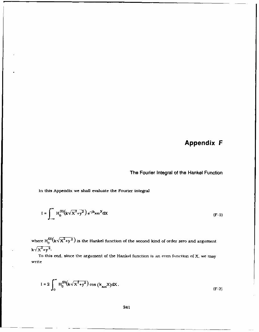
Appendix F

The Fourier Integral of the Hankel Function

In this Appendix we shall evaluate the Fourier integral

= H (2 (kV iy) e-jkxmxdX (F-1)

where H(2'(kN +y 2 ) is the Hankel function of the second klnd of order zero and argument2 .

To this end, since the argument of the Hankel function is an even function of X, we maywrite

1 2 jo Ho (k1+i) cos (k X)dX. (F-2)

241

Furthermore, Eq. (F-2) can be transformed into

o=2 J J°(kV +y2) cos (kX)dX -J2 J Y°(kXV+ 3) cos (kmX) dX (F-3)

where JoVX+ ) and Yo(kV--+- ) are Bessel and Neumann functions of order zero and

argument kAF- i+y.The integrals In Eq. (F-3) are given in Reference 14 as

Co (ynqrygcos y,<kx < k,y>O0

xmJo(kW )cos(kX) dX - (F-4a)

sin (yIk -kj) 0<k <k.y>O

Y" o(kV +Y) cos (kx) dX- K(n,0 <k< kxm, y >0.

xm

Using these results we may write

_j Yk2-2x

2 O<k <k,y>O

xm

I j .0 (k<k 0 F-5)

242

if we define

1C=N~ xm k > (F-Ga)

and

_____ = 2 <k2 - (F-Gb)

in Eq. (F-5). then Eq. (F-i) becomes

1 H~(kVrX + ) CJkxdX =2 e-.FGc

243

Appendix G

The Stationary-Phase Method for Evaluation of Integrals

Expressions for the first-order asymptotic evaluation of finite integrals of the type

(J) b f(x) e -Ja q(x) dx, (G-1)

xa

are listed below, where the large parameter Q1 Is assumed to be positive and qx) is a real

function of the real variable x. If the function f(x) has no singularities near an isolated first-

order stationary phase point x, of q(x), where q'(x,)=O. q"(x )* 0. the asymptotic

approximation of I{l) is given by (see Reference 13 for details)

'(!a) - s(f) u[(x3 - x)(,,- x)] + /2) + . a-3. (G-2)

245

where U(a) = 1 or 0 for ot > 0 and a < 0. respectively. The I is the lowest-order contribution

from the stationary-phase point, namely

f(X ) e 1q(. .X)Z0A/fl Q 8 fx) -J qxs J4. q"x (0 G-3a)

and Ie(fl) is the lowest-order contribution from the endpoints,

(1) = - 1 [f(Xb) eJQq(xb) - f(Xa) ejflq(a. (G-3b)le(l = Q P'-- t-- q'(x.) 1J"

The stationary point x, (at which q'(x) = 0) is assumed to lie on the interval x. < xs < xb; if the

interval contains several stationary points, sufficiently far apart, 5(nl) is a sum comprising

terms representative of each x.. When the saddle point coincides with either of the end points

Xa or xb, the corresponding endpoint contribution in Eq. (G-3b) is omitted and one takes 1/2

times the stationary-point contribution in Eq. (G-3a. When the interval x, < x < xb does not

contain a stationary point, the Heaviside function vanishes and the integral 1(fl) is

approximated by le(Q) only. When an endpoint moves to infinity, the corresponding

contribution is omitted. Relation (G-2) fails when the saddle point x. approaches one of the

endpoints; for example when x. moves continuously toward and across xb, the 1(U) term Is

discontinuous since the saddle point disappears from the integration interval, and the Ie(n)

term diverges, since q (xb) -+ 0 as xb -4 x,. In this Instance, one requires a more careful

asymptotic evaluation that involves the error function or the Fresnel integral.

246

Appendix H

Test for Power Conservation

In this Appendix we shall demonstrate that the expressions for the active array field due to

an infinite array of monopoles radiating into a semi-infinite parallel plate region satisfy theconservation of power condition.

All elements are fed with the same amplitude and progressive phase, exp(- kxo pd). This

permits one to apply the periodic-structure approach, in which the analysis reduces to a single

unit cell shown In Figure H-1. The unit cell consists of a single monopole radiating into arectangular wavegulde with conducting top and bottom walls and phase-shift side walls

characterized by Floquet's boundary conditions. The unit cell size is d x h where as already

mentioned h < X/2 so that in the semi-infinite parallel plate waveguide. only the TEM (n = 0)radial mode propagates. Also in this Appendix. for simplicity of presentation but with no lossof generality, we assume that the inter-element spacing d < ?/2. In this case only the

dominant (m = 0. n = 0) Floquet mode propagates In the unit cell. Moreover, to obtain thefinal conservation of power relation analytically in a closed form. it is assumed that the

probe current has only a single term (see Section 4.3).

The conservation of power relation may be stated as

247

Pnc( -Ir -(8 2) (H- 1)

Here

PInc -VtncI 2 Yc (H-2)

is the TEM mode incident power in the feed-coaxial transmission line with characteristic

admittance Yc. As indicated in previous sections, ra represents the active reflection coefficient

defined by Eq. (4-48a). In Eq. (H-I), Pt represents the far-field radiated power within a unit

cell of cross section area d x h. It Is given by

Pt -- /Re 2 E ×** yo dxdz. (H-3)

248

S i PHASE-SHIFTIc- - - - V F 2 - - - -S W A L L S

x~f (a)

z

S

h P - - Pt CONDUCTING

hJ I £ WALLS

y

t lal- - (b)

Pinc

Figure H- 1. Top (a) and Side (b) View of the Unit CellPertaining to Evaluation of the Complex Poynting Vector

To demonstrate Eq. (H-i) we may refer to a typical unit cell in Figure H-1. in which weconsider a volume V bounded by a surface S and containing TE ' -mode (double prime) fields.

From the complex Poynting Vector Theorem. the time-average power transnmtted across aclosed surface S Is given by the integral of the real part of the normal component of the

complex Poynting vector E W that is,

249

Ref. Ex fi* dS 0 (H-4)

since there are no sources inside S. In Eq. (H-4) d S = n dS is a vector element surface area

directed into the volume V. The surface S consists of the surface Sc around the unit cell

conducting walls, the unit cell side walls S1, S2 , the terminal plane S t. and the surface over the

aperture and probe area S. and S., respectively. It is assumed that the reference plane S t s

sufficiently far from the radiating element so that only the dominant mode field exists there.

The contribution to the surface integral over the conducting walls is zero since E x d S, = 0.

The contribution to the surface integral over unit cell side walls, as will be shown, is also zero.

This is due to the periodic property of the field, namely,

E(x+dy,z) = E(x,y,z) e -ikm (H-5)

and the fact that the normals on the opposite unit cell side-walls point in opposite directions

(into the volume V). Relation (H-5) is statement of Floquet's Theorem where the transverse

wave numbers of the Floquet modes are

k = kx o + 2 m m = 0, ±1'... (H-6)

With the help of Eq. (H-5). we write

jkd/2 = ' -~ejkxdE(d/2,y,z)ek = E(-d/2,y,z)e-Jk 12 (H-7a)

and

fik z) k d/2 ^Jxn/

H(df2,y,z)e 1 = (-d/2,y,z) e-Jk . JH-7b)

Consequently

250

E x H dS, = E(d/2,yz) x HW*(d/2.yz) dS1 = fE(-d/2yz) x fi*(-d/2,yz) * dS 1 . (H-8)

Since d S1 = -x o dy dz -d S2 in Eq. (H-7), one may write

J(-d/2.y,z) x H*(-d/2,yz) * dS 1

= -f2E(-d/2,yz) x H*(-d/2.y.z) * dS 2 = -fJ x H * dS 2 . (H-9)

From Eqs. (H-8) and (H-9) it follows that

JExH'dS 1 + Exf'dS2-0 (H- 10)

and therefore there is no contribution in Eq. ((H-4) due to the surface integral over the unit cellside walls S, and S 2.

Consequently Eq. (H-4) reduces to

Refs ExH ndS+ Ref ExH'.ndS + Ref , H'-9 ndSt 0. (H-I)J p ,/t

As noted earlier E and E denote the same active array field in the parallel plate region. The Erepresents the active array field in terms of cylindrical radial modes (see chapter 4) while Erepresernts the active array field in terms of Floquet modes in the unit cell (see Chapter 5). In

this Appendix both representations will be used, depending which is most convenient.Equation (H-I l) can be further simplified by noting that

251

fsExH* ndSa= J (nxM) xH*ndSa= [M(H * n) - n(H* -M)] o n dSa (H-12)

where the relation for the aperture field E = n x M has been used. Since H* • n = 0, Eq. (H-12)

becomes

s Ex H"-fndS=- H* MdS. (H- 13)

Here M Is the magnetic ring current given by

M= 0 o = 0oM a p5b. (H-14)p In~-a

Similarly. on the probe surface J = zo Jz(z) = n x H and therefore

f E xH n dS fE x G*xfn) 9 ndS= J[J* (E e n) - n (E J*)1 n ndS P(H- I5a)Sp P P

or

fsEXH* ndSp=-J, E JdS p (H-15b)

since J* (E * n) = 0. Thus. Fq (H- 11) may be written as

Re fs H* MdSa+Re f, E-JXdSp=RefsE x *YodSt. (H-16)

s p t

252

In the following three sections we will evaluate the integrals in Eq. (H-16) and show that Eq.(H- 16) holds. This verifies the expressions and the relation between the two representationsmentioned above for the active array fields introduced in Chapters 4 and 5.

HI EVALUATION OF THE COMPLEX POYNTING VECTOR OVER THE COAXIAL

APERTURE AREA

We start from the first integral in Eq. (H-16) which can be written as

2,, b=Re HI'I**MdS =Re f H; (p.z=O+) M, pd pd (H-17)

When Eq. (H-14) is used for M4. Eq. (H-17) becomes

2nV(z--o b] "I a Re H,' (p,z=) d p. (H- 18)a lnab Pa

The Integral in Eq. (H-18) Is given by Eq. (4-43) as

b KV(z=-) a r.,,b

fH;,'( pz : ° dp= LC . a - (2)

I I ,- +L ] , S,(+ (H- 19)

253

where V' and S. (8.) are defined in Eqs. (4-45h) and (4-47d), respectively.

For simplicity we shall assume that the probe current has a single term. In this case Eqs.

(4-46) apply, that is,

V' = C'I(H-20a)n In

where

x-2 21 Xn

2 X2- 21 h

i'n (il,= (H-20b)

21 h

and

Bc1 Ic '= A (H-20c)

Here c'I and C 1 are real and

Ai X £ -(~)1ona) [IH(2 (xna) + JoQcna S '6~) t2 (H-21a)

BI J d 0 (a) Ifn + .1. J81 .in H-2 ib)nn0

In view of Eqs. (H-20a) and (H-21b) when subsuituting Eq. (H-19) Into Eq. (H-18) vrields

254

_ Kj~~z= Re { [- [-a +In H'obo

_ Z 0_______ n

-n Jo( na) + j 2 Sn( 8)" - (c B1)} (H-22)

To determine the real part of the sum in this relation we first examine Sn{8x). For this reason

it is convenient to write

'sx= S + J S. (H-23)

where 3nr and S,, are real and can be found simply from Appendix E. Since h < X/2, only

So(8x) ka = 0) has a real part. In fact, since d < X/2 only the m = 0 term In Eq. (E-15a) has a real

part. 'L; Is easy to see that

Sor 8) = -1 + 4 - sin 2 (ks cos ). (H-24)kd cos

Thus

Sr +jS , n =0Sn() S n _1 (H-25)

Based on the above discussion we conclude that only the n = 0 ierm In the sum of Eq. (H-22)

has a real part.

To obtain an expression Ior Re (c BI in Eq. (fi-18). we 1wlte

B, = Blr + J B! (H-26)

255

where BIr and Bli are real. Since h < X/2 from Eq. (H-21b) we see that

Bir Jo(ka),l . S(,)]fJo(ka) lO* 0 4 ^sin2 (ks Cos J (H-27)kd cos

Therefore

ReI ',* R (' ,-jc ) B, j l))= 'r Bir - c'11 Blf, (H-28)

Inserting Eq. (H-28) into Eq. (H-22) we finally obtain

KfV z=0- 2 l 2 B (H-29)a kZ ir B ir + C 1 1 .LJ 1 1 J. lH-2i9

H2 EVALUATION OF THE COMPLEX POYNTING VECTOR OVER THE PROBE SURFACE

We next consider the second integral in Eq. (H-16):

i=Re I E*J*dS (H-30)p p

p

Since evaluation of Ip Is similar to that of I above, our derivation will be brief. Since E (az)and J(z) have no angular dependence one has

Ip=21a Re 1= Ez(a,z) J :(z) dz. (H-31)

From Eqs. (4-20a) and (4-20b) for the single probe current term

256

J (z) =c 1 sln-E (z - 1). (H-32)

The total tangential field on the probe surface is given by Eq. (4-22a) as

E z(a~z) = JK V0 (z = Oj-) (R n- P1l ;) C(z) (H-33)n0o

where the functions Rn and Pn are defined In Eqs. (4-22b) and (4-22c), respectively. The I1' is

given by Eq. (4-24a) as

V= c'l i (H-34a)n I I

where, from Eqs. (4-24b) and (4-24c)

k in -A kCzsni(z -1) dz (H-34b)

and

21ca ZH-401 V(Z=O1)1 (-3C

Substituting Eq. (H-34a) Into Eq. (H-33) and subsequently Eqs. (H-32) and (H-33) Into Eq. (H-31)

we have

I e K V 0(z O-)2iraI R j k-~-- (R~j-P.c, 1 1 ,) c* I 1 H-5

p n=0

257

Using Eq. (H-28) we may write

KJVo(Z -- o-)12 1 Cc P 1 112I)[ta aI =KvO Re{= O - c22 (H-36a)

or in terms of A, 1 and B1 defined by Eqs. (4-27b) and (4-27c) as

- 2A2IPnLI (H-36b)

BI= R In (H-36c)n---n

I becomesp

KJVo (z = 0-) 2 Re_-I-IC 12A

K zOI{lB I2A} (H-36d)

Since [see Eq. (4-27a)

- BI (H-37a)All

we see that

258

K IV.(z = 0-)12 e BIB*, BIB*[- €--Re IB = 0. (H-37b)

P kZ 0 A*, A*,,

Thus the integral of the complex Poynting vector over the probe surface is zero, as It should be.The boundary conditions for the field on the probe are therefore satisfied.

Although lp = 0. we rewrite Eq. (H-37b) into the form useful in the following analysis. We

start from Eq. (H-36d) which can be rewritten in the form

I KIV o (z - o )I (= ' , , t 2 )-p kZ 0 (r 1 Bt ' r + I I lr H3a

where Eqs. (H-20c) for c' (H-26) for BI and

Al * All +J Al (H-38b}

have been used. Since h < X/2 and d < X/2 it is easy to see that

Ar = It 2 Jo (ka)[ Sor(x) 12 (ka) 4 l2 (kd cos

kd cos

Ir.serting Eq. (H-39) into Eq. (H-38a) we obtain

KIV0(z=o0 2 { B 1 +c B - C, 212 oJo(ka)[1 + Sor(8)] 0. (H-40)

We shall now sum Eqs. (H-29) and (H-40), that is

I +1 -- 2 ( o -2c' + 12 (ka)1; ((-4i1a P kZ ° 0 ir r 1o+S (H-4

259

Substitution of Eq. (H-24) for Sor(61 ) and Eq. (H-27) for Blr, and the relation

1i0 '2 I, 12 i 0 (H-42a)

into Eq. (H-41) yields the final result

I +I=Re H** MdS +ReJ E'J*dS =Re fH**MdS a

a p a

kjV0 0 r J 0 (ka) 1 0 0 (ka)] s2 (ks cos )(H-42b)

kZo kd cos 0

H3 EVALUATION OF THE COMPLEX POYNTING VECTOR OVER THE UNIT CELLCROSS-SECTION AREA

In this section we evaluate the power through the terminal plane S t . which is given by the

integral

Pt = Ref X H* YodS t . (H-43)dt

We first list expressions relevant to the modal representation for the electromagnetic field

in the unit cell. As already mentioned, the latter consists of a single monopole radiating intoa rectangular waveguide with conducting top and bottom walls and phase-shift side walls

defined by Floquet type boundary conditions. Denoting the transmission direction by y In aCartesian coordinate system, the transverse field components due to a probe current and

magneic ring source in a unit cell with dimensions h x d may be expressed in terms of a

complete set of TE Y modes (double prime) asmn

260

Et(r)= V V" (y) Cmn(x.z). (H-44a)m=- n=0

m=-- n=0 m nm (H-44b)

The normalized vector mode functions are

e" (XZ) = -Z xm ejkx COSV _ !z (H-45a)okxJ VJ h h

and

h"(xz) = Yo x i em(xz) (H-45b)

where

l,n=OE = 12,n> 1 (H-45c)

Relations (H-45) represent a complete, orthonormal set such that

d/2 Ii

" ." F e" • ". dx dz = 8mn" m' 'in em'n mn. mfl H-6d/2 Jo

and similarly for the ii" functions. The asterisk denotes the complex conjugate and

stands for the standard Kronecker delta function. Modal voltage and current amplitudes

261

V" an I i I II

and I" satisfy the transmission-line equationsn mn

dnnI)- Z" I" (Y) (H-47a)

dy irn n M

d I" (y)0)n J Y" V" (H-47b)dy mn mn mn

where the modal characteristic impedances Z" and admittances Y" and the modalmn mn

propagation constants ic are defined by

- 1 - ° (H-47c)

mn

K k-ktn ,Im {Ixmn} 0. (H-47d)

The choice of sign on the square root insures the radiation condition for y -- c Here ktrm is

the transverse propagation wave vector

ktrm = x0 kxm + z0 kzn (H-48a)

with

ktuMn = Ik n IVk+-2 (H-48b)

where

262

k d= (H-48c)

and

k = n, n = 0, 1 .... (H48d)zn h

In Eq. (H-48c). kod = 8, where 8, is the inter-element steering phase delay.

For the dominant mode field (m = n = 0), Eq. (H-44) takes the fonn

Et(r) = V0 0 0) eo 0 (x) (H-49a)

Ht(r ) = Ioo (y) hoo (x) (H-49b)

where from Eq. (H-45a)

kxo e-jkxoX (H-49c)

Since

100 = Yoo Voo (H-50a)

we can see from Eqs. (H-49) and (H-46) that Eq. (H-43) may be written as

2

S '0 Y2o 0 (H-50b)

263

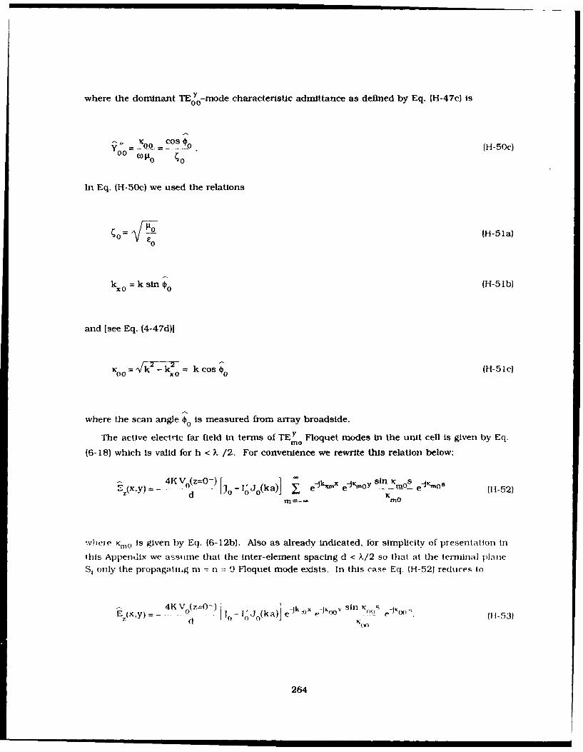
where the dominant TE Y-mode characteristic admittance as defined by Eq. (H-47c) is

000K" 0-Cos o

Yo -0 = (o H-50c)

In Eq. (H-50c) we used the relations

= o (H-51a)

k o = k sin 0 (H-5ib)

and [see Eq. (4-47d)

K = l kz_ :: k cos (H-10 ic)

where the scan angle o is measured from array broadside.

The active electric far field in terms of TE y Floquet modes in the unit cell is given by Eq.

(6-18) which is valid for h < X /2. For convenience we rewrite this relation below:

4KVO(Z=-) snEz(xY) =- d - IoJo(ka)j eJitmx ej oyiY - mO (Jos 1H-52)

rn=-- MOin

where Krn(, is given by Eq. (6-12b). Also as already indicated, for simplicity of presentation in

this Appenuix we assume that the inter-element spacing d < X/2 so that at the terninal planeSt only the propagating i = n = 9 Floquet mode exdsts. In this case Eq. (H-52) reduces to

zy 4K V (z=O-) I(ka) eJk.x JKo sin S eJ(i 11-53)- 0 1 , J e0(1

dI 0 0KW

264

We would like to cast Eq. (H-53) into the formr of Eq. (H--49a). Comparing these two relations

we see that

V0 0 ) =4KV (z=O-)i/h k tQ1 [3-IJ 0 ka)] si (H-54) 00

xOO( 00 0'CO(-4

From here

21I 012 16 le IV(=O_ 2 hj 3 2~ i 0(ka) -j30 1',J 0 (ka) + 11I12 .j2 (ka)j K

Koo

Since

one may write

1216K2 IV 0(Z=o- 2 2_ 1,22 1i 2 KO00"1 = K d [o -23 0 J0 (ka) Ciro t 0 j JO(ka) si2~ 0 (H-56b)

The real transmitted power through the terminal plane St can be now evaluated from Eq. (H-5(',)) where the domninant mode characteristic admittance is defined by Eq. (H-50c).Suibstitution of Eqs. (H-56b) and (H-50c) into Eq. (H-50b) yields

_t Ioz 2 h J - 2 10 Jo (ka) Clir 1 10o + 0 kd0(k

Dogerting Eq. (4-5d) for K into Eq. (H-57) we finally obtain

265

PtfKIV (z=o- 2 _2 1 o Jo(ka)ci, 11O + Ii 12 J2(ka) 4 sin 2 (ks cos ) (H-58akd cos ;o

where

o In [-(H-58b)Zo =2n a

We see that Eq. (H-58a) is identical to Eq. (H-42b) and therefore we conclude that Eq. (H- 16)is indeed satisfied. The latter relation is directly related to the conservation of powercondtion [Eq. (H- 1)] by the requirement that the complex power across a coaxial aperture mustbe continuous. Namely,

Vo(z=O-) Io(Z=O- ) = j_ H* * M dS. (H-59)a

Since, as shown in Section H2

Ref E .J*dSP = (H-60a)

one sees that

Vo(z=O-) 1o(Z=O-) = Pt' (H-60b)

The TEM mode voltage and curTent amplitudes V. and I Isee Eqs. (4-36) and (4-37)] in tile feed

coaxial transmission line can be expressed in terms of incident and reflected TEM modevoltages and currents Vin e . Vref, and linc, Iref , and the active reflection coefficient ra(8x) as

follows:

266

Vo(z=o-) Vt,,(z=o-) [I + ra(s) ] (H-61a)

10 (z=O-) = linc (Z=O -) -Iref(Z=0-) (H-6 Ib)

Using the identities

Vre =r a(6X) Vinc (H-62a)

I Ync YC Vt., (H-62b)

Iref - c Vref (H-62c)

one may write

V Vo- = (v o- v:.o 10* Vo 0 -c I ) c c ref) (H-62d)

Inserting Eqs. (H-61a) and (H-62a) into Eq. (H-62d) we obtain

vo lo = I Vinc 2 y [ 1 + r (a1 [1 - r: (a '] = I v~ 12 r I, r I(8.)12] (H-63a)v~~ x A H6a

where

I VJ 2n 1y c = P int H-63b)

represents the incident power in the feed transmission line. From Eqs. (H-60b) and (H-63) we

see that

267

P ic [1-_ I r( )12] =-pt (H-64)

which is the desired conservation of power relation. Thus, the expressions for the active array

field derived in Chapters 4 and 5 indeed satisfy the conservation of power condition.

268

Appendix I

Numerical Evaluation of the Integral [(a) = I f(x) e-Jlxdx

In this Appendix we consider the problem of evaluating numerically the integral

b= f(x) e-JaXdx (I

where the function f(x) is specil'ed at a finite number of equally spaced sampling points, anda is a large parameter. Since the integrand is a rapidly varing function of x. standard

numerical integration techniques cannot be applied because -1 the large number of integration

steps required to achieve a desired computational accuracy.

To develop an efficient integration scheme we assume that fix) is given by a set of values

{f(x,)}. i = 1.2.....N+l on the interval [a.bI where

269

b-a!= a +Q(- 1) N(1-2)N

and N is the number of subintervals. We approximate flx in each subinterval by a cubic

polynomial

P+x= C0.1 + C 1 (x-x ) + C 2 ,t(x-xi)2 + C 3 ,1(x-x) 3 (1-3)

with coefficients Cn.1 , n=O.....3, 1=1....N to be determined.

Hence one can write

b N x1+f(x) e-j~ x dx - P(x) e -J x dx. (1-4)I i=l fx i

It is Important to mention that the integrals in Eq. (-4) can be evaluated in closed form and

consequently the integration error is due only to the approximation of ijx) in each subinterval

by a cubic polynomial Pj(x}. The interpolation error Is estimated in Reference 12.

The method of determining P1(x) is known as cubic spline interpolation and is described in

Reference 12. The method is based on the requirement that

P(x,) = f(x) V -5a)

PI(x+ ) = f(x) (I-5b)

and

270

" " ... .II I I= =OImIi

p (X,) ="(.xi) (1-5d)

P ;'(X, 1,) = f'(x1 1,) (1-5e)

wl th I=1.N.From Reference 12 the coefficients Cnj are

C0.1 =fRx1 ) (1-6a)

= Ax~1 Ax,.x I + Ax1 fi x]

" 2j flxi.x,~i - C t- C 3tAxt(-)

. Ax ,IfI6

0111j~ + Cl~, - 2 flx,x,+3(I6d

3,1 (Ax) 2 (-d

where

Ax1I =+ 1 - xi (-6e)

and 1=1,.N+1.

The standard difference function is

f Xo f(x,,) (1-7a)

271

X1 -- 7b)x-x

o

or In 2x ge er l =f 2'I fX -X2 -f[Xn'X, ]

or in general

f[X n- .. x ] = f n - x .xn..n. 0n (1-7d)

Rewriting Eq. (1-3) Into the form

P1(x) = Ao + ALI x + A 2 3 x2 + A 3 x -a)

where

A =C2 -- C 3 (1-8b)0.1 01 C .3 - 21i x 32 3,1b)

A1 =C -2C 2 x +3 C3 x (I-8c)

A2 t =C 2 1 - 3 C3 .1 xI (1-8d)

Aa3, = C 3,1 (1-8e)

Eq. (1-4) becomes

ob N Xt+ I n_ dx I9

J f(x) e- j Oxdx = A n.1 xneUXdx.)1=2 n=O7

272

The integrals In Eq. (1-9) can be evaluated analytically using the general formula from

Reference 14

x eJOxdxJ xn e-J nx + Jn x (n + l ) e-J x dx. (1-10)

For the special case of

l(a) = fa f(x) e -J n x dxU- 1a

where f(x) is an even function of x, Eq. (I-1 la) reduces to

I(Q) = 2 f(x) cos O2x dx. (I- Ib)

In this case

N 3 xi+Xf(x) cos fx dx= X 1 An x' cos 1x dxJ 1=1 n=O (Ii12a)

where A nJ are given by Eq. (1-8) and

xn cos Q x si n f xr n, snx ,

fI 1 Q (I- 12b)

Specifically, the integrals In Eq. (I-12b) are

273

cosOx x sin Q, - sin Olx,

SfQ (I- 13a)

xi cos~ - cos f 1 1 sin a 1 + sin fx

f tIx cos fQx dx = cos i , I - o x x+ I sin x,+ + i Qx

St 2 Q 0- 13b)

2+1 cos = C xi cos Ox,JX+l X2 COS bdx=- il £X~

t l2

+sn D.,+, -v -2- sin Ox Y- 13c)

and

x~~co X1I _ 6~ x1+

+ - sin flx,+ 1 3 x sin Ox

Setting x=kxo, 12 = pd and f(x) = d/n ra(kxo). Eqs. 1-12) and (1-13) can be applied to e-aluate

the coupling coeflliclents for the infinite linear array of monopoles in the parallel plate

wavegulde as defined by Eq. (4-52).

274

MISSION

of

Rome Air Development Center

S RADC plans and executes research, development, test andselected acquisition programs in support of Command, Control,Communications and Intelligence (C1I) activities. Technical andengineering support within areas of competence is provided toESD Program Offices (POs) and other ESD elements toperform effective acquisition of C3I systems. The areas oftechnical competence include communications, command and

control, battle management information processing, surveillancesensors, intelligence data collection and handling, solid statesciences, electromagnetics, and propagation, and electronicreliability/maintainability and compatibility.

;e le ;_11 e-

LINEAR PHASED ARRAY OF COAXIALLY- FED MONOPOLE …

Documents

Transcript of LINEAR PHASED ARRAY OF COAXIALLY- FED MONOPOLE …