LINEAR GOAL PROGRAMMING IN CLASSIFICATION

AND PREFERENCE DECOMPOSITION

Kim Fung Bruce Lam

B. B. A. (Hons. 1, Simon Fraser University, 1984

M. B. A. , Simon Fraser University, 1986

THESIS SUBMITTED IN PARTIAL FULFILLMENT OF

THE REQUIREMENTS FOR THE DEGREE OF

DOCTOR OF PHILOSOPHY

in the Department

of

ECONOMICS

O Kim Fung Bruce Lam 1991

SIMON FRASER UNIVERSITY

November 1991

All rights reserved. This work may not be

reproduced in whole or in part, by photocopy

or other means, without permission of the author.

APPROVAL

Name :

Degree :

Title of Project:

Bruce Lam

Linear Goal Programming in Classification and Preference Decomposition

Examining Committee:

Chairman : Dr. L. A. Boland

Dr. E. U. Cnoo Associate Professor, Business Administration Senior Supervisor

Dr. A. R. Warburton Associate Professor, Business Administration

Dr-. W. Wedley Professor, Business Aaministration Internal/External Examiner

Dr. A. Stdm, Dept. ot Mgmt. sclences University of Georgia External Examiner

Date Approved: ,&,em& 25, /74/

PARTIAL COPYRIGHT LICENSE

I hereby grant to Simon Fraser University the right to lend my thesis, project or

extended essay (the title of which is shown below) to users of the Simon Fraser

University Library, and to make partial or single copies only for such users or in

response to a request from the library of any other university, or other educational

institution, on its own behalf or for one of its users. I further agree that

permission for multiple copying of this work for scholarly purposes may be

granted by me or the Dean of Graduate Studies. It is understood that copying or

publication of this work for financial gain shall not be allowed without my written

permission.

Title of Thesis/Project/Extended Essay

Li near Goal Programming i n Cl assi f i cati on and

Preference Decom~osition

Author: (signature)

Kim f-unrc Bruce Lam (name)

November 25, 1991 (date)

ABSTRACT

Linear programming approaches in multivariate analysis have

been studied by many researchers. In this work, linear

programming approaches in classification and preference

decomposition will be discussed. New and improved models in both

classification and preference decomposition will also be

introduced.

Classification addresses the problem of assigning objects to

appropriate classes. The two main classes of classification

approaches are cluster analysis and discriminant analysis.

Cluster analysis concerns the 'grouping' of 'similar' objects to

initially undefined classes. The main purpose of performing

cluster analysis is data simplification. Discriminant analysis

concerns the 'separation' of objects from several known

populations. The primary purpose of performing discriminant

analysis is to assign new objects to the correct population. Many

method5 including heuristic approaches and statistical approaches

have been proposed to solve the two classes of classification

problems.

In cluster analysis, heuristic approaches do not guarantee

optimal solutions with respect to any criterion. As a result,

various mathematical programming models for cluster analysis have

been developed. The advantage of mathematical programming models

is that they provide optimal solutions for specific optimization

objectives. I develop five new mathematical programming models in

cluster analysis. A published data set is used to examine the

performance characteristics of the cluster solutions obtained from

my models and six other clustering procedures. Six criteria

including five different measures of within cluster distances and

one measure of between cluster distances are used to evaluate the

cluster solutions obtained from the eleven models. All my models

provide better cluster solutions than the heuristic approaches.

iii

In discriminant analysis, the objects in the sample data set

are from known populations. Popular statistical approaches to

discriminant analysis are Fisher's discriminant function and

logistic regression. Linear programming approaches in

discriminant analysis are known to be robust and have been shown

to have competitive performance when compared with the other

statistical approaches. In this work, two new linear goal

programming models in discriminant analysis are being introduced.

The first model incorporates the within group discriminate

information which is usually ignored by the other techniques in

discriminant analysis. The classification performance of this

model and several other popular discriminant techniques are

evaluated by both an empirical study, which is based on the actual

experience of an MBA admission committee, and a simulation

experiment. The second model allows non-monotonic attributes to

be included in the estimation process. In order to evaluate the

classification performance of the second model and the other

approaches in discriminant analysis with non-monotonic attributes,

a simulation experiment is being conducted. Classification

performance of the models in discriminant analysis are evaluated

by the hit-ratio, the number of objects correctly classified. My

models perform well in the above experiments.

Preference decomposition is a class of methods used to

measure a respondent's multiattribute preference structure.

Usually, a set of well selected alternatives is presented to a

respondent who then expresses hidher preferences for the

alternatives in terms of either nonmetric or metric measurement.

Then, based on the overall preferences of the alternatives,

preference decomposition is used to estimate the individual's

preference function. I introduce a linear goal programming model

for preference decomposition with the input preference judgments

measured in ratio scale. In order to compare the predictive

validity of my model and two other models, LINMAP and Ordinary

Least Squares, a simulation experiment is being conducted.

Performances of the models are evaluated by both the Pearson

correlation coefficients and Spearman rank coefficients between

the input preferences and the derived preferences of the

alternatives. Both my model and Ordinary Least Squares have

higher average Pearson correlation coefficients and average

Spearman rank coefficients than LINMAP in this experiment, while

the coefficients of my model and Ordinary Least Squares are close

to each other.

In summary, I introduce several new linear goal programming

models to solve the problems in cluster analysis, discriminant

analysis, and preference decomposition. The five new models in

cluster analysis provide additional optimization objectives to

modelers in cluster analysis. This increase in the flexibility in

choosing alternate optimal objectives in cluster analysis will

likely motivate more frequent applications of mathematical

programming approaches to cluster analysis. My first model in

discriminant analysis incorporates the within group discriminate

information. Intuitively, this model may provide more accurate

estimations of the attribute weights than the other techniques

which ignore the within group discriminate information. My second

model has the ability to incorporate non-monotonic attributes in

discriminant analysis. The existing linear programming approaches

in preference decomposition only allow the input preference

judgments to be measured in ordinal scale. Theoretically, ratio

scale preference judgments contain more information than ordinal

scale preference judgments. Consequently, I introduce a linear

goal programming model which allows the input preference judgments

to be measured in ratio scale.

TABLE OF CONTENTS

APPROVAL i i

ABSTRACT iii

LIST OF TABLES vii

1. INTRODUCTION 1

1.1 Cluster Analysis 1.2 Discriminant Analysis 1.3 Preference Decomposition

2. MATHEMATICAL PROGRAMMING APPROACHES TO CLUSTER ANALYSIS 5

2.1 Introduction 2.2 The Problem of Grouping 2.3 Hierarchic Methods 2.4 Systematic ways of generating Criteria for

Cluster Analysis 2.5 Mathematical Programming Approaches to Cluster

Analysis 2.6 Computational Example 2.7 Conclusion Appendix 2.1:' Formulations of SM and SW

3. LINEAR GOAL PROGRAMMING IN DISCRIMINANT ANALYSIS 21

3 .1 Introduction 2 1 3.2 The Problem of Separating groups 2 1 3.3 Linear Goal Programming in Estimation of 2 8

Classification Probabilities 3.4 A Linear Goal Programming Model for Classification 40

with Non-monotone Attributes 3.5 Conclusion 48 Appendix 3.1: Listing of 68 Cases 5 0 Appendix 3.2: Listing of SPSS-X Programme 5 1

4. LINEAR GOAL PROGRAMMING IN PREFERENCE DECOMPOSITION

4.1 Introduction 4.2 Review of Preference Decomposition 4.3 Model Formulation 4.4 Simulation Experiment 4.5 Conclusion

5. CONCLUS I ON

REFERENCES

LIST OF TABLES

Inefficiency of Cluster Solutions from different Methods

List of Attributes and Labels

Group Attributes and Indicator Weights

Attribute Weights of the Different Methods

Classification Results of the Different Methods

Average Hits of Different Methods (First Simulation Experiment)

Average Hits of Different Methods (Second Simulation Experiment)

Total Average Hits in the Two Simulation Experiments

Average Hit Rates of all the Methods

A Symmetrical Orthogonal Array for the 34 Factorial Design

The Part-Worth values wke obtained from (GPD) and the

original attribute values yke

4.3 Average Pearson correlation coefficient and average Spearman rank coefficient of GPD, LINMAP, and OLS

CHAPTER I

INTRODUCTION

The goal programming model was first proposed by Charnes,

Cooper, and Ferguson [19551. Their work has motivated many

applications of using linear programming techniques in

multivariate analysis including multiple regression, cluster

analysis, discriminant analysis, and preference decomposition

[e. g. , Wagner, 1959; Vinod, 1969; Rao, 1971; Srinivasan and

Shocker, 1973; Freed and Glover, 1981al. In this work, linear

goal programming approaches to problems in classification and

preference decomposition are being studied. The two main types of

classification techniques are cluster analysis and discriminant

analysis. The later concerns the 'separation' of objects from

several known populations while the former concerns the grouping

of 'similar' objects to initially undefined classes. Preference

decomposition is a class of methods used to measure an

individual's multiattribute preference structure given the

individual's relative preferences of some chosen alternatives.

New and improved models in both classification and preference

decomposition will be introduced.

1.1 CLUSTER ANALYSIS

Cluster analysis has been applied in many fields of

scientific inquiry, in business, in industry, and in education.

Many heuristic methods have been proposed to solve the clustering

problems. Unfortunately, the heuristic methods do not guarantee

optimality with respect to any criterion. As a result, various

mathematical programming models for cluster analysis have been

developed. The objective functions of mathematical programming

for cluster analysis are usually defined as measures of either

"within cluster distances" or "between cluster distances". With

an analog of multicriteria optimization framework, I provide a

systematic way of generating a whole array of meaningful criteria

for cluster analysis. We also introduce five new mathematical

programming models and reformulate two existing models in chapter

2. A published data set is used to examine the performance

characteristics of my models and several other popular clustering

procedures.

1.2 DISCRIMINANT ANALYSIS

Recently, linear programming approaches to discriminant

problems have been widely studied and have been shown to yield

satisfactory results. In chapter 3, I introduce two new linear

goal programming models in discriminant analysis. The first model

works directly with the conditional probabilities of group

membership rather than the simple group category to which a member

belongs. With the use of conditional probabilities, the strength

of group membership is measured and further discrimination within

group is possible. Both an empirical data set which is obtained

from an M.B.A. admission committee and simulated data are used to

test the effectiveness of the above linear goal programming model

and the other popular classification methods for discriminant

analysis in minimizing misclassification errors. Since the

primary purpose of performing discriminant analysis is to assign

new objects to the correct population, the performance of the

methods are evaluated by the hit ratio, the number of correctly

classified objects.

Classification of objects are based on their overall scores

computed from the classification function. However, according to

the classification function, the higher the attribute score of an

object, all other factors being equal, the higher (if this

attribute has a positive weight in the classification function) or

the lower (if this attribute has a negative weight in the

classification function) is its overall score. This implied

monotonicity is not reasonable in many situations. The second

model I introduce is a linear goal programming model which has the

ability to incorporate non-monotonic attributes in discriminant

analysis. A simulation experiment is conducted to examine the

effectiveness of this goal programming approach to classification

problems with and without non-monotonic attributes.

1.3 PREFERENCE DECOMPOSITION

In choosing the best alternative with respect to multiple

criteria, it is a common practice to determine the criterion

weights which influence the preference of all the alternatives

presented. The criteria are aggregated into a single preference

function and the alternative with the highest preference function

value is identified as the optimal choice. The preference

function values can also be used to rank order all the

alternatives. However, many decision makers are able to make

preference judgments based on the alternative as a whole without

any detailed criteria trade-off. To understand the choice

behavior of these decision makers, it is pertinent to evaluate how

they value the alternatives' criterion levels. Preference

decomposition is a class of methods used to decompose the overall

preference of alternatives into part-worth evaluations of

criterion levels. Given the input judgments of preference among

some carefully selected alternatives, the additive preference

decomposition estimates a part-worth value for each level of each

criterion. The sums of the part worths which correspond as

closely as possible to the input preferences are used to determine

the preferences among all alternatives. Theoretically, ratio

scale preference judgments contain more information than ordinal

scale preference judgments. Consequently, in chapter 4, I

introduce a linear goal programming model for preference

decomposition where the input preference judgments are measured in

ratio scale. I conduct a simulation experiment to compare the

predictive validity of my model and two other models namely LINMAP

and Ordinary Least Squares in estimating the preference function.

Performance of the models are evaluated by both the Pearson

correlation coefficients and Spearman rank coefficients between

the input preferences and the derived preferences of the

alternatives. Both my model and Ordinary Least Squares have

higher average Pearson correlation coefficients and average

Spearman rank coefficients than LINMAP in this experiment, while

the coefficients of my model and Ordinary Least Squares are close

to each other.

CHAPTER 2

MATHEMATICAL PROGRAMMING APPROACHES TO CLUSTER ANALYSIS

2.1 INTRODUCTION

The problem of

of objects into cer

cluster analysis is to partition a

tain appropriate classes such that

given set

it is

optimal with respect to a certain chosen criterion function. Many

heuristic methods have been proposed to solve the cluster analysis

problem. Unfortunately, the heuristic methods do not guarantee

optimality with respect to any criterion. As a result, various

mathematical programming models for cluster analysis have been

developed. In this chapter, I focus the discussion on the

mathematical programming approaches. In section 2.4, with an

analog of multicriteria optimization framework, I provide a

systematic way of generating a whole array of meaningful criteria

for cluster analysis. In section 2.5, I introduce five new

mathematical programming models, two of which are bicriterion

formulations. I also reformulate two existing mathematical

programming models which utilize fewer variables than the two

existing models. Computational results from a published data set

in cluster analysis are presented in section 2.6.

2.2 THE PROBLEM OF GROUPING

Problems of cluster analysis involve grouping a certain

number of objects into a certain number of clusters. Given a

sample of n objects, the most general problem in cluster analysis

is to group the n objects into clusters where the number of

clusters is not known. Many heuristic methods have been proposed

to solve the cluster analysis problems. The single linkage,

complete linkage, group average linkage, and Ward's Method are

some popular bottom-up hierarchic methods used in cluster analysis

[Blashf ield and Aldenderf er, 1978; Gordon, 1981; Johnson and

Wichern, 19881. In section 2.3, hierarchic methods will be

discussed. The hill-climbing and the k-means methods [MacQueen,

19671 are two iterative reassigning procedures. Unfortunately,

the heuristic approaches do not guarantee global optimality with

respect to any criterion. The inadequacy of the heuristic methods

has provoked the serious consideration of mathematical programming

approaches to cluster analysis [Vinod, 1969; Rao, 1971; Arthanari

and Dodge 1981; Aronson and Klein, 19891. The advantage of

mathematical programming models is that they provide optimal

solutions to specific optimization objectives. This is most

useful when an appropriate criterion for clustering exists. For

example, mathematical programming approaches have been

successfully applied to many location problems.

In cluster analysis, it is essential to define the distance

between each pair of objects in the data set. The distances

should reflect the "similarity" between pairs of objects. Usually

the objects within clusters are more "similar" than objects in

different clusters. Each object is typically described by a

vector of attribute values. The "similarity" between objects is

measured in terms of some distance metrics defined on the

attribute space. Let n be the number of objects in a data set, p

be the number of attributes, X be a nxp matrix which represents

the attribute values of the n objects in the p dimensional space,

and D be the distance matrix derived from X where d is defined i j as the distance between the i-th object and the j-th object. The

followings are the distances that are commonly used:

P i) City block metric: d. .= Ixik-xjk

lJ k=l I

ii) Euclidean metric: C

P iii) Minkowski metric: d. .=

positive integer.

iv) Weighted Minkowski distance:

r is a positive integer.

V) Weighted Tchebycheff metric: di j = Max wklxik-xjk .

1 sksp I

2.3 HIERARCHIC METHODS

The agglomerative approach is a popular class of hierarchic

methods. Agglomeration starts with n clusters with each cluster

contains only one object. Then at each stage, two closest

clusters are merged to form one cluster until finally all objects

are grouped into a single cluster. Different agglomerative

approaches differ by the ways they define the distance between two

clusters. The following are some distances between two clusters

defined by several common agglomerative hierarchic methods:

Single linkage: It is also called the nearest neighbor method.

The distance between two clusters is defined as the distance

between their nearest members. At each stage, the two

clusters with the smallest distance are merged.

Complete linkage: It is also called the furthest neighbor method.

The distance between two clusters is defined as the distance

between their furthest members,

Group average linkage: The distance between two clusters is

defined as the average of the distances between all pairs of

objects in the two clusters.

Wards' Method: It is also called the sum of squares method. In

this method two clusters are merged if the amalgamation leads

to the minimum increase in the total within cluster sum of

squares at each stage.

Hierarchic methods are easy to implement but may not produce

optimal solutions.

2.4 SYSTEMATIC WAYS OF GENERATING CRITERIA FOR CLUSTER ANALYSIS

Let m be the number of clusters embedded in the sample. Many

methods have been proposed to determine the number of hidden

clusters in a data set. Milligan and Cooper [I9851 have provided

a comparison study of thirty such procedures. However, when m can

be prespecified, the remaining task is to identify the clusters

according to some specific criteria.

There are many reasonable criteria which can be used in

forming clusters. Thus they lead to different objective functions

in the mathematical programming approaches. The structure in

multicriteria optimization can be used to develop a systematic way

of generating meaningful criterion functions for clustering

problems. Suppose n objects have been grouped into m clusters.

It is logical to evaluate the m clusters as follows:

For each k=1,2, . . . , m, let f be some measure of "deficiency" k of the k-th cluster. Typically, fk measures the "dissimilarity"

of all the objects in the k-th cluster. Alternatively, f may k measure the "closeness" from the k-th cluster to other clusters.

It is obvious that we want to "minimize" F=(f f ..,fm), which 1' 2"

is a multicriteria optimization problem. A common approach to

solve this multicriteria optimization problem is to "combine"

fl,f2, ..., f into one single overall objective function. Let g be m

a real valued function defined on the m-dimensional space of f k values, k=1,2,. . . ,m, such that g(fl, f . . . , f 1 measures the

2, m

overall "badness" of fl,f2, ..., fm. Then the problem can be solved

by minimizing g(fl,f 2,...,fml. There are many acceptable ways to

define the cluster "deficiency" fl,f2, ... ,f and the overall value m function g [Chankong and Haimes 19831. In this paper, I consider

m - the weighted sum (WS), g(fl,f2,. . . ,fm) = wkfk, and the k= 1

Tchebychef f norm (TF) , g (f l, f 2, . . . , fm) i MAX {wlfl, . . . , w f ), m m where w1,w2,. . . ,wm are positive numbers which reflect the relative importance of the m clusters respectively. To avoid considering

too many different forms of g(f f ..,f ) , seven ways of 1' 2" m defining f l, f2, . . . , f are considered: m

a. SDM: Sum of distances from objects to cluster medians,

b. MDM: Maximum distance from objects to cluster medians,

c. SDC: Sum of distances from objects to cluster centers,

d. SWD: Sum of within cluster pairwise distances,

e. MWD: Maximum within cluster pairwise distance,

f. MSW: Maximum sum of within cluster distances from an object,

g. NSB: -(Minimum sum of between cluster distances from an object)

Note that NSB is defined with negation so that fk is to be

minimized. There are 14 (=7x2) different forms for

g (f l, f2, . . . , fm) . For convenience, SDM-WS is used to denote

g(fl,f2, ..., fm) when f f .,f are sum of distances from 1' 2'" m objects to cluster medians (SDM) and g is the weighted sum (WS)

function. Theoretically, each form of g(fl,f2, . . . , fm) can be taken as the objective function to be minimized in a mathematical

programming model for cluster analysis. Furthermore, we may

combine two or more objective functions together and solve the

problem as a new multicriteria problem. Thus many cluster

analysis models can be generated. I will introduce two

bicriterion models in the next section. Among the 14 basic

models, the following have already been studied:

1. Vinod [I9691 and Aronson & Klein [I9891 use SDM-WS.

2. Rao [I971 I uses SWD-WS. 3. Rao [I9711 uses MWD-TF.

Discussing all fourteen models will be too lengthy and some of the

models may not be as intuitively attractive as the other models.

For example, both MDM and MUD measure "maximum distance" in a

cluster. If we use US for g(f ,f , f 1, then in some optimal 1 2'"' m solutions, some clusters may have large "maximum distances" while

other clusters may have small "maximum distances". These results

may be difficult to interpret. It is more meaningful to use TF

for g(fl,f2, . . . , fm) such that g(f f 1' 2'"'

.fm) can be interpreted

as the "overall maximum distance" in all the clusters. Therefore,

for illustration purpose, I only look at one model for each of the

seven definitions of fk.

The fundamental question in cluster analysis is what makes a

good cluster solution. Evaluation of cluster solutions must,

therefore, be based on some meaningful criteria. The different

forms for g(fl,f2, ..., fm) can be used as criteria in evaluating the cluster solutions. In Section 2.6, we will compare the

cluster solutions obtained by different clustering models based on

the values of these criteria.

2.5 MATHEMATICAL PROGRAMMING APPROACHES TO CLUSTER ANALYSIS

For all the models discussed in this section, I use the

following variables for cluster memberships:

1 if the i-th object belongs to the k-th cluster z ik 0 otherwise

For models (SDM-US) and for i=l, . . . ,n and k=l, . . . ,m. (MDM-TF), the variables used

as follows:

Yik = { 1 if the i-th ob, 0 otherwise

to identify the medians are defined

ject is the median of the k-th cluster

for i=l,. . . ,n, k=l, . . . ,m. Since the models (SM) [Vinod, 19691 and (SW) [Rao, 19711 use different variables, I reformulate their

models in this section.

2.5.1 Cluster-Median Problem

One of the objective functions for the mathematical

10

programming methods in cluster analysis is to minimize the total

sum of distances from each object to the "representative" point

(cluster median) of the cluster in which the object belongs. If

it is restricted that only the n sample points can be chosen as

the cluster-medians, then this problem is usually called the

cluster-median problem [Vinod 19691. This objective function

shares the same or similar objectives of some location problems

[Revelle, Marks and Liebman, 1970; Ghosh and Craig, 1986; Church,

Current and Storbeck, 19911. For example, if we wanted to build

three shopping malls to serve twenty suburban areas, we would like

to build the shopping malls in certain locations such that the

total sum of distances travelled from the twenty areas to their

nearest shopping malls is minimized.

Vinod 119691 formulated the cluster-median problem as an

integer programming problem (SM) (the formulation is in Appendix

2.1). I reformulate (SM) as follows:

n (SDM-WS) MIN C hi

i=l n

S.T 1 dijyjk - M(l-zik) - h i " 0, for k=l, . . . , m (2.2) j=l i=l,. . . ,n

for i=l, . . . , n ( 2 . 3 )

for k=l,. . . ,m (2.4)

h. 20, 'ik zero-one and z zero-one. 1 ik

M is a large positive number. When z equals to zero, the ik corresponding constraint in (2.2) becomes redundant. When z ik equals to one, h. is forced to equal to d where point j is the

1 i j median (yjk=l) of cluster k. Constraints in (2.3) enforce that

each object must be belonged to one cluster. Constraints in (2.4)

identify exactly m medians.

2 . 5 . 2 The Problem of Minimizing the Overall Maximum Distance from

an Object to Its Median

Considering the cluster median problem, a different objective

is to minimize the overall maximum distance from an object to its

median. I formulate this problem as follows:

(MDM-TF) MIN H

S.T. dijyjk - M(1-zik) - H 5 0, j=l

for k=l,. . . ,m (2.6) i=l,. . . ,n

for i=l, . . . , n (2.7)

for k=l, . . . , rn (2.8)

HrO, yik zero-one, z zero-one. ik

In (2.6), the variable H captures the overall maximum distance

from an object to its median. Let the optimal objective value of * * (MDM-TF) be H . Since H equals to the overall maximum distance

from an object to its median, multiple solutions are likely to

exist. Multiple solutions exist when the distances from an object

(or several objects) to two or more medians are less than or equal * to H . If this occurs, then this object (these objects) can be * assigned to different clusters without affecting the value of H . However, among the multiple solutions, some solutions may be more

preferred than the others. In order to choose the "best"

clustering solution among the multiple solutions, I formulate the

problem as the following bicriterion problem:

(MDM-TF-B) MIN PIH + P2( 1 hi) i=l

S. T. di jyjk - M(1-z 1 -hiso, for k=l, . . . , m (2.10) j=l ik

i=l,. . . ,n for i=l, . . . ,n (2.11)

for i=l, . . . , n (2.12)

for k=l, . . . ,m (2.13)

HrO, hirO, yik zero-one z zero-one. ik

In (MDM-TF-B), P is preemptive over (i.e. much larger than) P 1 2

and H is forced to be equal to the maximum value of h in (2.11). i The first priority goal of (MDM-TF-B) is the same as the objective

in (MDM-TF), while the second priority goal is the same as the

objective in (SDM-WS).

2.5.3 The Problem of Minimizing the Sum of Distances from Objects

to the 'Centers'

For the cluster median problem, there is no intuitive reason

to restrict the medians to be located on the sample points only.

A more general problem is to relax this restriction by allowing

any point in the p-dimensional attribute space to be the medians.

Revelle, Marks and Liebman [I9701 classified this type of problem

as "Location on a Plane" in location analysis. It allows for more

flexibility in the locations of the medians. I formulate this

problem as a mixed-integer programming problem (SDC-WS) in the

next section.

Consider the cluster-median problem where any point in the

p-dimensional attribute space can be selected as a cluster median.

Let (b kl,...,b be the k-th median. Using city-block distance kp

to define the distances between the sample points and the medians,

this problem can be formulated as follows:

n P (SDC-WS) MIN Z hij

i=l j=l

- b -M(l-z -h 5 0, for i=l,. . . ,n (2.15) S.T. Xij kj ik ij j=l,. . . ,p

b - xi -M(l-z ) -hij 5 0, for i=l, . . . ,n (2.16) kj ik j=l,. . . ,p

k=l,. . . ,m for i=l,. . . ,n (2.17)

bkjzO, hijtO, z zero-one. ik

Constraints (2.15) and (2.16) are linear forms of the following

conditions:

-M(l-z ) -hij 5 0, for i=l, . . . ,n (2.18) ik j=l,. . . ,p

Although (SDC-WS) allows for more flexibility in the location

of the medians, with large values of n, m, and p, (SDC-WS) will be

a large mixed integer programming problem which is difficult to

solve. Hence, (SDC-WS) is more suitable to solve small to

moderate size problems. Nevertheless, with small size problems,

there is an apparent advantage of (SDC-WS) over (SDM-WS). If the

locations of the medians can be chosen only from the sample

points, then the smaller the sample size, the less will be the

possible locations to locate the medians. As a result, choosing

good "representative" medians for the clusters became a more

difficult task in (SDM-WS). However, the number of possible

locations in (SDC-WS) is still infinite even when the sample size

is very small.

2.5.4. The Problem of Minimizing Within Cluster Distances

Another objective is to minimize the total sum of pairwise

distances between objects in the same cluster. Rao [I9711

developed a zero-one integer programming model (SW) for this

problem (the formulation is in the Appendix 2.1). However, (SW)

is difficult to solve because it has too many zero-one variables

and constraints. Aronson and Klein [I9891 provided an improved

mixed-integer programming model, (SWl), which contained fewer

variables than Rao's model (the formulation is in the Appendix

2.1). They applied their model in the area of computer-assisted

process organization for information development.

I reformulate this problem as a mixed-integer programming

problem (SWD-WS) which has fewer variables and constraints than

both (SW) and (SW1). My model is as follows:

n (SWD-WS) MIN C hi

i=l

n S. T. 1 dijzjk - M(1-z. -hi a 0, for i=l, ..., n (2.201 lk j=l k=l,. . . ,m

for i=l, . . . , n (2.21)

hihO, z zero-one. ik

In (2.20), when zik equals to one, h. measures the sum of 1

distances of object i to the other objects in the same cluster.

If zik equals to zero, then the corresponding constraint becomes

redundant. The number of variables and number of constraints in

(SWD-WS) are both equaled to mn+n, and are much less than (SW) and

2 . 5 . 5 The Problem of Minimizing the Overall Maximum Within

Cluster Distance

Rao [I9711 introduced a zero-one integer programming model

(MWD-TF) to solve the cluster problem by minimizing the overall

maximum pairwise distance within cluster. The formulation is as

follows:

(MWD-TF) MIN H (2.22)

S. T. dijzik + dijzjk - H 5 dij, for 1 , . . 1 (2.23) j=i+l, . . . , n

for i=l, ..., n (2.24)

HZO, z zero-one. ik

If both zik and z equal to one, then H is forced to be greater J k than or equal to d in (2.231, or H must be equal to the largest

i j pairwise distance in the same cluster. However, similar to the

problem of (MDM-TF) in section 2.5.2, multiple solutions may exist.

Since if the distances from an object to the objects in more than * one cluster are less than or equal to H , then this object can be

assigned to any of those clusters without affecting the value of * H . I formulate a new model (MWD-TF-B) which chooses the 'best'

clustering solution among the multiple solutions is as follows:

(MWD-TF-B) MIN PIH + P2( C hi) i=l

S.T. dijzik + dijzjk - H 5 d for i=l,. . . ,n-1 (2.26) ij, j=i+l,. . . ,n

1 dijzjk - M(1-z. )-his 0, for i=l, ..., n (2.27) j=l lk k=l,. . . ,m

for i=l, . . . , n (2.28)

HrO, hiZO, z zero-one. ik

P is preemptive over P (MUD-TF-B) is an improved version of 1 2' (MWD-TF). The first priority goal of (MWD-TF-B) is to minimize

the overall maximum within cluster distance, same as the objective

in (MWD-TF), while the second priority goal is to minimize the sum

of pairwise distances as in (SWD-US).

2 . 5 . 6 The Problem of Minimizing the Maximum Sum of Distances from

One Object to Other Objects Within Cluster

In this section, I define the "dissimilarity" measured in a

cluster as the maximum sum of distances from one object to the

other objects within the same cluster. The objective function of

the corresponding model is to minimize the sum of the

"dissimilarity" measured in all the clusters. I formulate this

problem as follows:

m (MSW-US) MIN 1 hk

k=l

S.T. 1 dijzjk - M(1-Z. 1 -hk" 0, for i=1, . . . , n (2.30) j=l

lk k=l,. . . ,m

for i=l, . . . , n (2.31 1

hkrO, z zero-one. ik

In (2.30), h is forced to be greater than or equal to the maximum k sum of within group distances. Consequently, h captures the sum k of the within group distances to the worst cluster median. The

sum of h over all clusters is minimized. k

2.5.7 The Problem of Maximizing the Minimum Sum of Distances from

One Object to the Other Objects in Different Clusters

Another possible objective in cluster analysis is to maximize

the overall minimum sum of distances from one object to all the

other objects in different clusters. I formulate this problem as

follows:

(NSB-TF) MIN -H (2.32)

S. T. d i k 1 - z . )+H s lk 1 dij, for i=l, ..., n (2.33) j=l j=l k=l,. . . ,m

HrO, z zero-one. ik

for i=l, ..., n (2.34)

In (2.33), the value of H is less than or equal to the smallest

sum of between cluster distances. If zik equals to one, then H

must be less than or equal to the sum of between cluster distances

for object i. Again, if zik equals to zero, then the

corresponding constraint in (2.33) becomes redundant.

2.6 COMPUTATIONAL EXAMPLE

In this section, I apply the above methods and some popular

heuristic methods in cluster analysis to a problem, and examine

the cluster solutions obtained from the different methods. The

data set I use is a distance matrix from Johnson and Wichern

11988, p.5461. This distance matrix describes the distances

between twenty-two utilities. I apply six mathematical

programming models; (SDM-WS 1, (MDM-TF-B 1, (SWD-WS) , (MWD-TF-B 1,

(MSW-WS) and (NSB-TF), (the model (SDC-WS) is excluded due to the

large problem size), and five heuristic methods namely, between

groups average linkage (BGAVG), within group average linkage

(WGAVG), single linkage (SINGL), complete linkage (COMPL), and

Ward's method (WARD) to the data. I use six forms of

g(fl,f2, . . . , f ) to evaluate these methods. After I obtained the m

cluster solutions from all the methods, I calculate the six

criterion function values for all these cluster solutions and the

results are reported in Table 2.1.

Table 2.1: Inefficiency of Cluster Solutions from different Methods

CRITERIA MODELS SDM-WS MDM-TF SWD-WS MWD-TF MSW-WS NSB-TF AVERAGE

(SDM-WS) 0.000* 0.053* 0.148 0.079* 0.097 0.386 0.127 (MDM-TF-B) 0.015* 0.000* 0.046 0.162 0.038* 0.112* 0.062 (SWD-WS) 0.055 0.061 0.000* 0.162 0.014* 0.089* 0.064 (MUD-TF-B) 0.111 0.095 0.018* 0.000* 0.069 0.139 0.072 (MSW-WS) 0.073 0.167 0.010* 0.162 0.000* 0.148 0.093 (NSB-TF) 0.161 0.350 0.083 0.162 0.065 0.000* 0.137 ( BGAVG 1 0.051 0.090 0.628 0.144 0.135 0.731 0.297 ( WGAVG ) 0.051 0.090 0.628 0.144 0.135 0.731 0.297 (SINGL) 0.072 0.090 2.059 0.144 0.175 0.905 0.574 ( COMPL ) 0.070 0.294 0.075 0.079* 0.091 0.281 0.148 (WARD) 0.008* 0.053* 0.244 0.079* 0.108 0.519 0.169

Note: Asterix represents the best three approaches in each criterion function, and 0.000 represents the best approach.

For each of the criterion functions, it is expected that the best

method is the mathematical programming model which gives optimal

solution. Note that none of the heuristic methods performs better

or as well as any of the mathematical programming approaches. It

is interesting to see that for the mathematical programming

models, their solutions also perform well when evaluated by the

other criterion functions. For example, (MDM-TF-B) is one of the

top three methods in four out of the six criterion functions, and

each of (SDM-WS) and (SWD-WS) are one of the top three methods in

three out of the six criterion functions. Other mathematical

programming models also perform well in the other criterion

functions. This is reflected by the average values of

inefficiency from the eleven models in Table 2.1. The average

values of inefficiency of the six mathematical programming models

are significantly less than that of the heuristic methods.

2.7 CONCLUSION

The main advantage of the mathematical programming approaches

to cluster analysis is the capability of providing an optimal

solution with respect to some appropriate obJective functions. I

provide a systematic way of generating a whole array of meaningful

criteria for cluster analysis. In particular, I introduce five

new mathematical programming models, including two bicriterion

formulations. The ability to generate many meaningful criteria

for evaluating cluster solutions increases the power and the

flexibility of applying mathematical programming approaches to

cluster analysis. The computational results support the use of

mathematical programming models in cluster analysis. Additional

constraints [Aronson and Klein, 19891 can easily be incorporated

into the models.

Appendix 2.1: Formulations of (SM) and (SW)

According to Vinod [19691, the cluster-median problem can

be formulated as follows:

1 if the i-th objects belongs to the j-cluster Let xi 0 otherwise

for i=l, . . . ,n and j=l, . . . ,n.

(SM) MIN Z dij xij i=1 j=1 n

S.T. xij=lD j=l n

xjj=m j=l

n

for i=1,

for j=l,

x zero-one. i j

In (SM), the number of clusters defined is n, where n-m clusters

are empty. In (2.371, only m of the x are equal to 1 (if xj j=l, .I .J then point j is a median) and the other x are equal to zero.

j j The constraints in (2.38) define non-empty clusters.

Rao [I9711 discussed an integer programming model, (SW),

which has the objective of minimizing the sum of within group

pairwise distances. Let

k 1 if both i-th and j-th objects belong to the k-th cluster Yij = { 0 otherwise. His formulation is as follows:

k Yi j

zero one, z zero-one. ik

for 1 , . . 1 (2.40) j=i+l,. . . ,n k=l, . . . ,m

for i=l, . . . , n (2.41)

k Aronson and Klein [I9891 modified (SW) by replacing all yij ,

for k=l, ...,p in (SW) by yij. I call their model (SW1).

CHAPTER 3

LINEAR GOAL PROGRAMMING IN DISCRIMINANT ANALYSIS

3.1 INTRODUCTION

In this chapter, two linear goal programming models to

discriminant analysis are being introduced. The first model

incorporates discriminating information within group in terms of

group membership probabilities in a linear goal programming model.

The second linear programming model has the ability to capture the

non-monotonicity of the attribute scores in discriminant problems.

The two models are discussed in section 3.3 and 3.4, respectively.

A review of some common techniques in discriminant analysis:

Fisher's discriminant function, logistic regression, and linear

programming approaches is presented in the next section.

3.2 THE PROBLEM OF SEPARATING GROUPS

Discriminant analysis concerns separating two or more groups

of objects in a data set and allocating new objects to previously

defined groups. Generally, we start with m random samples from m

different populations, of sizes n n n Eachobject is 1' 2'"" m' typically described by a vector of attribute values. For a

classification problem with two populations n and n 1 2' classification of objects is based on the measurements on p

attributes. The sample data matrices for population 1 and

population 2 are A and A2, respectively. 1

3.2.1 Fisher's Linear Discriminant Function

For a two-group classification problem, Fisher [I9361

attempted to take a linear combination of the p attributes, and

choose the coefficients to maximize the ratio of the between group

variance to the within group variance. He developed the following

sample linear discriminant function:

where ; and ; are the sample mean vectors of A and A2, 1 2 1

respectively, S is the pooled sample covariance matrix, and a is

the vector scores of an object. The classification rule based on

the samples becomes the following: - - ' -1 - - ' -1- -

Classify a to nl if (a -a ) S a z 1/2(al-a2) S (al-a2) 1 2 - - ' -1 - - ' - 1 - -

Classify a to n2 if (al-a2) S a < 1/2(a 1 2 -a 1 S (al-a2).

Fisher's linear discriminant function will minimize the

probability of misclassification if the following conditions are

met:

1. The population distributions are multivariate normal.

2. The covariance matrices of a and a are the same. 1 2 3. The means and the common covariance matrix are known.

This has been a very popular approach used in discriminant

analysis.

3.2.2 Logistic Regression

The logistic regression follows from the Bayes's Theorem:

where i=1,2 in a two groups discriminant problem. If p(alni ) and

P(n. ) are known, then ~ ( n ~ l a ) can be computed. However, p(alni) 1

and P(n ) generally need to be estimated. i

If one assumes the conditional probability density function

takes the following form [Day and Kerridge, 19671:

where €)(a) is a non-negative scalar function of a and 8(a) is

integrable, and r >O is a normalizing constant, then i

There are two approaches to estimate 6 and p'. One is the 0

weighted least-square approach and the other is the maximum

likelihood approach [Flath and Leonard, 19791.

3.2.3 Mathematical Programming and Discriminant Analysis

Since Freed and Glover [1981a, 1981bl and Hand [I9811

proposed the use of linear programming approaches to solve the

discriminant problems, many authors [Bajgier and Hill, 1982; Choo

and Wedley, 1985; Freed and Glover, 1986; Stam and Joachimsthaler,

1989; Lee and Ord, 19901 developed different variants of the

linear programming models. Furthermore, some authors [Bajgier and

Hill, 1982; Choo and Wedley, 1985; Freed and Grover, 1986;

Joachimsthaler and Stam, 1988; Stam and Joachimsthaler, 1990; Stam

and Jones, 1990; Lee and Ord, 19901 attempted to compare and

evaluate the classification performance of the mathematical

programming approaches and statistical approaches via empirical or

simulated experiments.

The linear programming model introduced by Freed and Glover

[1981al has the objective to minimize the maximum deviation (MMD)

for the objects that are misclassified by the classification

function. Let X be a nxp matrix where xik denotes the k-th

attribute value of the i-th object for i=1,2, ..., n, and k=1,2, ...,p, where n is the number of objects in the sample, w be k the estimated weights in the classification function, where

k=l, . . . , p , and G and G be the two sample sets drawn from n and 1 2 1 n respectively. The (MMD) model is formulated as follows: 2'

(MMD) MIN d (3.8)

for icG1 (3.9)

for icG2 (3.10)

w c unrestricted in sign, drO. k'

In (MMD), a normalization constraint is needed to avoid the

trivial solution (i.e., the values of all wk and c equal to zero).

Freed and Glover [I9861 suggested the use of the following

normalization constraint:

where r is a non-zero number.

Instead of minimizing the maximum deviation, Freed and Glover

[1981bl proposed another linear programming model to minimize the

sum of individual external deviations (MSD). Let n = nl + n then 2' n

(MSD) MIN C di i=l

for ieG (3.13) 1

for ieG (3.14) 2

w c unrestricted in sign, dirO. k'

The objective of (MSD) is to minimize the total group overlap

instead of the maximum overlap as in (MMD). A normalization

constraint is needed in (MSD) to avoid the trivial solution.

The objective of minimizing the sum of interior distances

[Freed and Glover, 19861 can be formulated as the following linear

programming problem (MSID):

(MSID) MIN qld - q2 1 ai i=l

for icG1 (3.16)

for ieG2 (3.17)

w c unrestricted in sign, drO, a 20. k' i

(MSID) is a bicriterion linear programming model where the two

objectives are minimizing the maximum misclassification and

maximizing the sum of deviations of the correctly classified

objects from the cutoff boundary. The values of ql and q2 reflect

the relative importance of the two objectives in (MSID) and must

be provided by the decision maker.

Choo and Wedley [I9851 discussed the use of an integer

programming method to minimize the number of misclassified objects

in a classification problem. Their integer programming

formulation (MNM) can be stated as follows:

n (MNM) MIN 1 ei

i=l

for icGl (3.19)

for i€G (3.20) 2

a, wk unrestricted in sign, e zero-one. i

M is a large positive number, and e are zero-one variables for i all i. The objective of (MNM) is to minimize the actual number of

misclassifications.

Koehler and Erengue [19901, Stam and Joachimsthaler [I9901

also studied the problem of finding a linear discriminant function

to minimize the number of misclassifications. Their model (MNM2)

is as follows:

n (MNM2) MIN C ei

i=l P

(3.21 1

for icG1 (3.22)

for i€G2 (3.23)

w c unrestricted in sign, e zero-one. k' i

A normalization constraint is needed to avoid the trivial solution

in (MNM2).

Stam and Joachimsthaler [I9891 discussed the use of 8 norm P

in discriminant analysis. Their model can be expressed

as the following mathematical programming problem:

n (LPN) MIN 1 (diIr 1 (l/r 1

i=l

for i€G1 (3.25)

P

"kxik - di + ai = C, for ieG2 (3.26) k= 1

w unrestricted in sign, di=O, a 20, r is a positive integer. k i

The cutoff value c is chosen arbitrary. They pointed out that

(MMD) and (MSD) are the two special cases of the .! norm P

discriminant analysis. The (MMD) and (MSD) formulations are the

same as (LPN) formulation when r=w and r=l, respectively.

Another variant of the linear programming models was

proposed by Lee and Ord [19901. They formulated the

classification problem similar to a regression problem where the

objective function is to minimize the sum of absolute deviations

(LAD). The formulation is as follows:

n (LAD) MIN C (d + ail i i=l

P C wkxik + a + di - a = 1, i

for ieG1 (3.28) k= 1

5 .,xi, + a + d - a =0, i i for ieG2 (3.29)

k= 1

a, wk unrestricted in sign, dirO, a i 20.

There have been some attempts [Bajgier and Hill, 1982; Freed

and Grover, 1986; Joachimsthaler and Stam, 1988; Lee and Ord,

19901 to compare and evaluate the classification performance of

the mathematical programming approaches and the classical

discriminant techniques using simulated experiments. Some of the

results show that linear programming approaches are competitive

with the classical discriminant techniques in terms of the

classification performance (number of objects correctly

classified).

Bajgier and Hill [I9821 found that (MSD) and (MMD)

outperformed Fisher's linear discriminant function (FLDF) under

certain conditions of the data sets in a simulated study. The

(MSD) performed better than (FLDF) when the sample sizes of the

two groups were unequal. The (MMD) outperformed the other

approaches under the condition that group overlap was small, but

not performing well when the two groups were close to each other.

Freed and Glover [1986, pp.1611 reported their finding as " . . . Tests results showed that among the LP variants tested, the (MSD)

formulation generally is the most reliable predictor of group

membership". In their simulated experiment, Joachimsthaler and

Stam [I9881 found that when outliers were present in the data set,

(MSD) and logistic discriminant function performed better than

(FLDF). Koehler and Erengue [I9901 reported that (MNM2) performed

better than (FLDF) as the variance heterogeneity of the two

populations increased. The above results show that linear

programming approaches (especially the MSD) are competitive

alternatives to the classical discriminant techniques.

3.3 LINEAR GOAL PROGRAMMING IN ESTIMATION OF CLASSIFICATION

PROBABILITIES

The linear programming approaches to classification problems

have yielded satisfactory results [Choo and Wedley, 1985; Freed

and Glover, 1986; Glover, Keene and Duea, 1988; Joachimsthaler and

Stam 19881. Unlike logistic regression [Cox, 1970; Anderson,

19721, which can incorporate membership probabilities of an object

belonging to a group, linear programming models [Choo and Wedley,

1985; Freed and Glover, 1986; Glover, Keene and Duea, 1988; Lee

and Ord, 19901 and (FLDF), when applied to estimate the attribute

weights of the classification function, do not incorporate

discriminating information between members within the same group.

Group membership probabilities, when available, can be and

should be used to discriminate between members of the same group.

When working with categorical dependent variables, most methods

round off the group membership probabilities, and information

useful for discriminating between members within the groups is

lost. For example, dividing companies into bankrupt and

non-bankrupt groups ignores the fact that the non-bankrupt group

contains companies of varying qualities. This is a severe

disadvantage of (FLDF) and linear programming models where group

membership is coded as a dichotomous or categorical variable.

Recently, constrained multiple regression models with general

l -norm are used to estimate membership probabilities [Stam and P Ragsdale, 19901.

I provide a continuous goal programming model (GP1) which

works directly with the conditional probabilities of group

membership rather than the simple group category to which a member

belongs. In applying this continuous goal programming model to

classification problems, the users have to provide the estimated

group membership probabilities of the objects within the sample.

With the use of conditional probabilities, the strength of group

membership is measured and further discrimination within groups is

possible. Actual experience of an MBA admission committee is used

to illustrate the implementation of (GP1).

The classification power of (GP1) is compared with four other

methods of classification including logistic regression (LG),

(MNM) [Choo and Wedley, 19851, multiple regression with minimum

sum of absolute deviations (MSAD) [Wagner, 19591, and Fisher's

linear discriminant function (FLDF). Moreover, simulated data are

used to test the effectiveness of the above approaches in

minimizing misclassification errors.

3.3.1 Model Formulation

For the two groups discriminant problem with n objects

(n=n +n 1, let pi, i=l, . . . , n be the probability that the i-th 1 2

object belongs to one of the parent populations. The rows of X

are arranged in the descending order of the p values. i Furthermore, let wl, W2' ""

be the attribute weights to be P

determined and the weighted sum function w x +w x +. . .+ w x is 1il 2 i 2 P i~ used to distinguish the likelihood of belonging to the population.

In the perfect situation, the weighted sums w x +w x +. . .+ w x 1 il 2 i2 P i~ will have the same ordering as the p values and thus we would i expect the following :

There are n(n-1)/2 inequalities in (3.30). All these inequalities

are used in the ordinal regression [Srinivasan, 19751. However,

when IpU-PrI is small, it is not wise to enforce the corresponding

ordering in (3.30) due to possible data inaccuracy in pU and p r' Thus, unlike the ordinal regression, many pairwise comparisons

(u,r) may be excluded from (3.30).

There are many reasonable methods to select the subset of

pairwise comparisons to be enforced in (3.30). I suggest one

approach as follows:

For any small a>O, define Da by Da = { (u,r) : lsu<rsn,

pu-pr - 1 sa & pU-pr>a ). Essentially, D consists of consecutive a

pairs (u,r) with p -p slightly greater than a. Let ra = max {r : u r (u,r)€D for lsusn). Then none of the pairs in D includes any

a a r-th object with r>ra. To avoid this omission, define Ua = {(u,r)

: r +lsrsn, <a & p >a) when r <n and let % = Da u Ua . a Pu+ 1 -Pr- u-'r a

The n(n-1)/2 inequalities in (3.30) are replaced by

Since perfect ordering is not always possible, deviational

variables dur are introduced into (3.31) to allow for more

flexibility:

that the difference

The objective is to minimize the total sum of deviations

1 dur . Furthermore, it is natural

(u, TIER a P P

wkx& - wkxrk should be larger for k= 1 k= 1

The model formulation for

probabilities for all the

(GP1) MIN C dur (u, r)cR a

preserving the

pairs in R is a

larger values of p -p u r'

order of membership

given below:

S. T. i WkXuk - i wkxrk+dur Pu-P,, V (u,r)cRa (3.34) k=l k= 1

w unrestricted in sign, d 20, V(u, r)c% k ur

The attribute weights wl,w2, . . . , w obtained from the solution P

of (GP1) are used to compute the weighted sums wlxil+ w x + . . . + 2 i2

w x , i=1,2,. . . , n, of all the objects. The log odds ratio, P ip

ln(p./(l-pi) 1, i=1,2,. . . , n, of all the objects, is regressed on 1

the weighted sums to obtain an intercept coefficient b and a 0

slope coefficient b For any object i, its membership 1'

probability p. is estimated by 1

3.3.2 Additional Features

Sometimes, prior information may be available in a

classification problem. For example, the members in an MBA

admission committee may agree that the higher the GMAT score of an

applicant, the higher the probability that this applicant will be

accepted. Consequently, the attribute weight for the GMAT score

should be positive. Furthermore, the admission committee may also

agree that GMAT score is the most important factor in evaluating

applicants. Therefore, GMAT score should be weighted more heavily

than the other attributes in the classification function. In

practice, additional constraints reflecting useful prior

information can be added to (GP1) to obtain better and more

meaningful attribute weights. These include the positive or

negative sign constraints on the weights of certain attributes.

Let x be the average values of the k-th attribute in the k

development sample, then higher weights can be imposed on more

important attributes by adding the following constraint,

where T can be any desired value which reflects the relative

importance of the u-th attribute and the v-th attribute. Extreme

values of attribute weights can be avoided by bounding the ratios

of the attribute weights. For example, adding the following

constraints to (GP1) can avoid extreme values of attribute

weights,

with appropriate values of U and L.

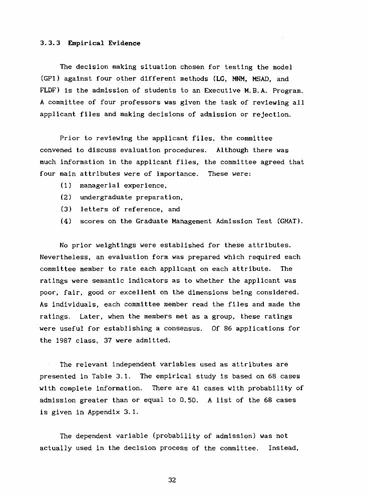
3.3.3 Empirical Evidence

The decision making situation chosen for testing the model

(GP1) against four other different methods (LG, MNM, MSAD, and

FLDF) is the admission of students to an Executive M.B.A. Program.

A committee of four professors was given the task of reviewing all

applicant files and making decisions of admission or rejection.

Prior to reviewing the applicant files, the committee

convened to discuss evaluation procedures. Although there was

much information in the applicant files, the committee agreed that

four main attributes were of importance. These were:

(1) managerial experience,

(2) undergraduate preparation,

(3) letters of reference, and

(4) scores on the Graduate Management Admission Test (GMAT).

No prior weightings were established for these attributes.

Nevertheless, an evaluation form was prepared which required each

committee member to rate each applicant on each attribute. The

ratings were semantic indicators as to whether the applicant was

poor, fair, good or excellent on the dimensions being considered.

As individuals, each committee member read the files and made the

ratings. Later, when the members met as a group, these ratings

were useful for establishing a consensus. Of 86 applications for

the 1987 class, 37 were admitted.

The relevant independent variables used as attributes are

presented in Table 3.1. The empirical study is based on 68 cases

with complete information. There are 41 cases with probability of

admission greater than or equal to 0.50. A list of the 68 cases

is given in Appendix 3.1.

The dependent variable (probability of admission) was not

actually used in the decision process of the committee. Instead,

it was determined afterwards. Each committee member used the

Analytic Hierarchy Process, AHP [Saaty, 19771 to determine weights

for the four main attributes and the four semantic indicators used

to rate each attribute. For example, each member had to think of

prototype candidates with poor, fair, good and excellent records

on managerial experience. Then with the managerial experience

attribute in mind, they undertook AHP paired comparisons between

prototype candidates to establish importance weights for the

semantic indicators. In a like manner, priority weight zik was

established for each indicator b with respect to each attribute k.

Finally, AHP comparisons were carried out to determine weight w k

for each attribute.

Table 3.1: List of Attributes and Labels

Name Description Type Labe 1

JOBL Job level C

YMGT Years in management R JOBS Job mobility I

DEG Highest education C

YEDD Years out of school I LETT Employer's letter C

QGMAT Quantitative score R TGMAT Total GMAT score R LETA Average reference C PROB Probability R

l=Non-business, 2=Consul tant , 3=Low, 4=Middle, 5=Top

Number of job title switches in last 5 years l=Non-university, 2=Some university, 3=technical college, 4=CPA/CGA, 5=CA/non-science graduatehon-business graduate, 6=B. Sc. , 7=B. Bus. , 8=Masters degree, 9=Ph. D. Number of years since formal education O=No. 1 to 6 indicating strength of reference. Quantitative GMAT score

Average strength of references. Acceptance probability.

C = Categorical variable, R = Ratio variable, I = Integer variable.

Using the indicator weights as absolute measures, each

candidate i has a score s i = 'wk Vk(61kizlk+62kiz2k+63kiZ3k+64kiZ4k) ' where abki=l means the candidate i was rated with indicator b with

respect to attribute k, and abki=O otherwise. This score s can i be used to measure the desirability of candidate i. Saaty calls

this use of AHP as measurement with absolute values. These

scores s are converted into probabilities of acceptance by i rescaling them between 1, the probability for an imaginary

candidate who scores excellent on all indicators, and 0, the

probability for another imaginary candidate who scores poor on all

dimensions.

Although it is possible to calculate the membership

probabilities perceived by each committee member, I have used the

average group ratings, importance weights, and indicator values to

emulate the group discussion, and consensus process which actually

occurred in the committee. Thus, I am using aggregated group

scores to generate the committee's probability of acceptance for

each candidate. The average attribute weights and indicator

values which were used in the study are given in Table 3.2. The

resulting acceptance probabilities are in the last column of

Appendix 3.1.

Table 3.2: Group Attributes and Indicator Weights

At tribute Group Indicator Weights Attribute

Weight Poor Fair Good Excel lent

Managerial .305 .076 .I48 .283 .493 Experience

Academic Pre~aration

.280

Letters of .095 .081 .I58 .313 .448 Reference

Highest

Lowest

Potential Score = .305(.493)+.280(.483)+.095(.448)+.320(.527) = .497, which is given a probability of 1.

Potential Score = .305(.076)+.280(.056)+.095(.081)+.320(.054~ = .064, which is given a probability of 0.

The data of 68 cases are randomly divided into development

and validation samples with 34 cases in each sample. For all the

methods used, attribute weights are derived from the development

sample. Then the remaining holdout sample is used to measure the

success of each method. Success is defined herein as the ability

of each method to correctly identify the candidates with greater

than or equal to 0.50 probability of admission. A listing of the

SPSS-X [I9881 programme used is given in Appendix 3.2.

All the attribute weights obtained by the various methods are

given in Table 3.3. The classification results are given in Table

3.4. (GP1) and (MNM) both have six misclassifications in the

validation sample. Both (LG) and (FLDF) have eight

misclassifications and (MSAD) has nine misclassifications in the

validation sample. (GP1) and (MNM) have the smallest number of

misclassifications in the validation sample.

Table 3.3: Attribute Weights of the Different Methods

-

ATTRIBUTE WEIGHTS JOBL YMGT JOBS DEG YEDD LETT QGMAT TGMAT LETA CONSTANT

METHOD (GP1) -.357 .I16 (RGP1) -.I98 .057 (LG) -.022 .024 ( MNM .510 .I47 (RMNM) 6.793 -1.19 (MSAD) -.017 .003 (RMSAD) -. 007 .003 (FLDF) -. 395 -. 030

Note that the attribute weights of DEG and LETT obtained from

(GP1) and (MNM) are both negative which seem to contradict

apparent intuition. But further analysis shows that applicants

with higher degrees may not always be preferred to those with a

Bachelor degree in Business (score 7). Applicants with either a

Master degree (score 8) or a Ph. D. (score 9) have usually majored

in areas other then Business and are not working at high

management levels. Furthermore, applicants who are either CPA/CGA

(score 4) or CA (score 5) may have a higher chance of being

accepted than those with Bachelor degrees in Sciences. Thus, the

sign of degree is really indeterminate. However, for LETT it is

difficult to interpret why the weight is negative.

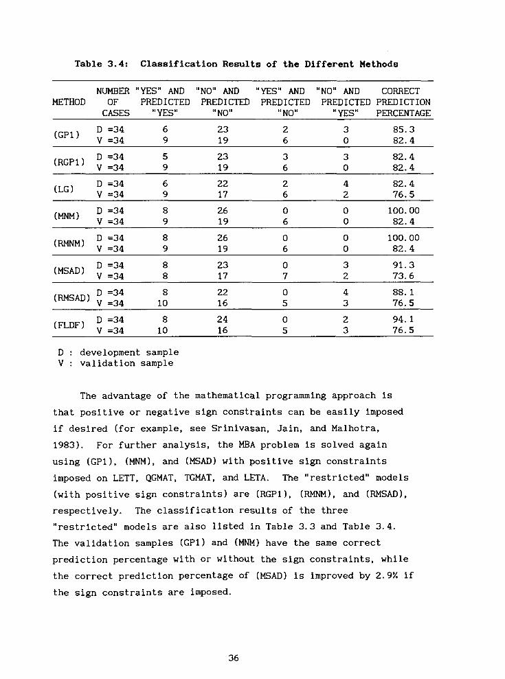
Table 3.4: Classification Results of the Different Methods

NUMBER "YES" AND "NO" AND "YES" AND "NO" AND CORRECT METHOD OF PREDICTED PREDICTED PREDICTED PREDICTED PREDICTION

CASES "YES" 'I NO" ,,NO" "YES" PERCENTAGE

D : development sample V : validation sample

The advantage of the mathematical programming approach is

that positive or negative sign constraints can be easily imposed

if desired (for example, see Srinivasan, Jain, and Malhotra,

1983). For further analysis, the MBA problem is solved again

using (GPl), (MNM), and (MSAD) with positive sign constraints

imposed on LETT, QGMAT, TGMAT, and LETA. The "restricted" models

(with positive sign constraints) are (RGPl), (RMNM), and (RMSAD),

respectively. The classification results of the three

"restricted" models are also listed In Table 3.3 and Table 3.4.

The validation samples (GP1) and (MNM) have the same correct

prediction percentage with or without the sign constraints, while

the correct prediction percentage of (MSAD) is improved by 2.9% if

the sign constraints are imposed.

3.3.4 Simulation Experiment

Two simulation experiments are conducted to investigate the

performance of the different classification techniques in

discriminating between groups. For both experiments, the samples

are drawn from two multivariate normal populations with three

discriminating attributes. Population 1 is distributed as N(0,I)

and population 2 is distributed as N(v,A), where v is a mean

vector and A is a diagonal matrix. Similar to Bajgier and Hill

[19821, the three means in v are chosen to be equal as are all the

diagonal elements in A. Three different values, 0.5, 1,and 3 are

chosen to represent three different mean vectors, and 1, 4, and 16

are chosen to represent the diagonal elements of three different

diagonal matrices. This yields a 3x3 factorial design with nine

combinations in each of the two simulation experiments. The

relative frequency of population 1 and population 2 are set to be

equa 1.

In the first simulation experiment, the linear sum of the

three attribute values of each object is perturbed and then

substituted into a logistic equation to compute the probability of

group membership. The probability of group membership is obtained

from the logistic equation. As a result, the experimental design

in the first simulation experiment is in favor of logistic

regression. The second simulation experiment tries to eliminate

this bias.

In the second simulation experiment the linear sum of the

three attribute values of each object is systematically

transformed using the following criteria: the highest 50% of the

linear sums are transformed into squares of the linear weighted

sums, and the lowest 50% of the linear sums are transformed into

square roots of the linear sums. After these transformations, the

linear sum is perturbed and then substituted into a logistic

equation to compute the probability of group membership. In both

simulation studies the linear sums are perturbed by adding a

random error which is normally distributed with zero mean and

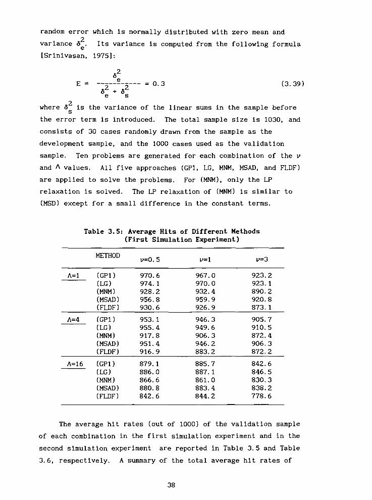
variance 6' Its variance is computed from the following formula e' [Srinivasan, 19751:

2 where 6 is the variance of the linear sums in the sample before S

the error term is introduced. The total sample size is 1030, and

consists of 30 cases randomly drawn from the sample as the

development sample, and the 1000 cases used as the validation

sample. Ten problems are generated for each combination of the v

and A values. All five approaches (GP1, LG, MNM, MSAD, and FLDF)

are applied to solve the problems. For (MNM), only the LP

relaxation is solved. The LP relaxation of (MNM) is similar to

(MSD) except for a small difference in the constant terms.

Table 3.5: Average Hits of Different Methods (First Simulation Experiment)

A= 1 (GP1) 970.6 967.0 923.2 (LG) 974.1 970.0 923.1 ( MNM 1 928.2 932.4 890.2 (MSAD ) 956.8 959.9 920.8 ( FLDF 930.6 926.9 873.1

A=4 (GP1) (LG) (MNM) ( MSAD ) ( FLDF

A=16 (GP1) (LG) ( MNM 1 (MSAD 1 ( FLDF 1

The average hit rates (out of 1000) of the validation sample

of each combination in the first simulation experiment and in the

second simulation experiment are reported in Table 3 .5 and Table

3.6, respectively. A summary of the total average hit rates of

the nine combinations in each simulation experiment are reported

in Table 3.7.

Table 3.6. Average Hits of Different Methods (Second Simulation Experiment)

v=O. 5 v=l v=3

A= 1 (GP1) 877.2 835.4 632.4 (LG) 874.7 835.5 628.2 ( MNM 1 847.1 803.5 632.7 ( MSAD 1 869.3 834.5 639.7 ( FLDF 1 860.6 818.7 627.3

A=4 (GP1) 694.8 648.0 585.4 (LG) 690.0 646.5 568.6 ( MNM 1 675.9 635.4 573.5 ( MSAD ) 675.5 642.0 569.5 ( FLDF 1 671.9 633.9 569.4

A=16 (GP1) 540.4 540.3 519.6 (LG) 539.6 534.4 518.2 (MNN 1 544.7 533.9 514.2 (MSAD ) 539.1 530.9 516.6 ( FLDF 1 546.9 529.3 516.7

Table 3.7: Total Average Hits in the Two Simulation Experiment

Met hod First Second Simulation Experiment Simulation Experiment

In the first simulation experiment, logistic regression has

the best performance in term of the average hit rates. Since the

original membership probability is computed from a logistic

equation, this result is expected. (GP1) has the second highest

average hit rate, and (MSAD) has the third highest average hit

rate.

In the second simulation experiment, (GP1) has the best

performance in terms of the total average hit rates. (LG) has the

second highest average hit rate and (MSAD) has the third highest

average hit rate. It should be pointed out that the systematic

non-linear transformation of the linear sum of the attribute

values in the second simulation experiment does not seem to favor

any of the five approaches. In summary, (GP1) has performed well

in this simulation experiment.

3.4 A LINEAR GOAL PROGRAMMING MODEL FOR CLASSIFICATION WITH

NON-MONOTONE ATTRIBUTES

Statistical approaches and linear programming approaches to

classification problems presume monotonicity of the attribute

scores with respect to the likelihood of belonging to one specific

group. This may not be realistic in many applications. In view

of this, I propose a general linear programming approach with the

ability to capture the non-monotonicity of some attribute scores

in classification problems.

3.4.1 The Problem of Non-monotonic Attributes

Objects are classified based on the overall scores computed

from the derived classification function. However, according to

the classification function, the higher the attribute score of an

object, all other factors being equal, the higher (if this

attribute has a positive weight in the classification function) or

the lower (if this attribute has a negative weight in the

classification function) will be its overall score. This implied

monotonicity is not reasonable in many situations. For example,

if the age and blood pressure of an individual are being used to

determine whether to assign an individual to a "beginners" fitness

class or to an "advanced" fitness class, then an individual who is

either too old or too young and an individual who has either a

high blood pressure or a low blood pressure may not be suitable

for the "advanced" fitness class. As a result, neither positive

weights nor negative weights are suitable for both the age and the

blood pressure attributes in the classification function. Similar

examples can be found in some medical diagnoses when high

attribute scores or low attribute scores may indicate symptoms of

certain diseases. One possible approach to overcome this

difficulty is to transform the scores of an monotonic attribute as

deviations from the "desirable value" for the class, however,

sometimes desirable value may not be easy to determine. Moreover,

there may exist a range of "desirable values".

In the next section, a linear goal programming model (GP2)

which can overcome the difficulty of imposing an implied

monotonicity in classification function analysis is developed.

Furthermore, a simulation experiment is conducted to examine the

effectiveness of this linear goal programming approach to

classification problems. The results of the proposed approach are

very encouraging.

3.4.2 Model Formulation

As noted earlier, Fisher's linear discriminant function,

logistic regression, and linear programming approaches do not

handle cases with non-monotonic attribute scores (attribute scores

which are not monotonic with respect to the likelihood of

belonging to a specific population). In order to overcome this

problem, the following approach is suggested. We first consider

the case when all the attribute scores are non-monotonic in a two

groups discriminant problem. For non-monotonic attributes, their

scores are discretized into at least two different levels. Let gk

be the number of levels for the k-th attribute, and

( 1 , if the level of the k-th attribute of the i-th object

( 0 , otherwise

where k=l, . . . ,p, C=l, . . . ,gk, and i=l, . . . ,n. Let wke be the weight of the t-th level of the k-th attribute in the classification

function. The overall score of any object i is equal to

wke6ie. Equivalently, we can replace each attribute k by g k=l e=i k

dummy variables 6 &l, ...,g in the matrix X. Let c be the cut kt' k

off value of the overall score between G and G The goal is to 1 2'

determine a set of weights, w for k=l, . . . , p, e=l,. . . , gk, kt which

satisfies the following conditions:

for ieG1 (3.40)

P gk i

C C Wke6ke I c, for ieG2 (3.41) k=l e=i

Since perfect classification results may not always be possible,

deviational variables di and a can be introduced to allow for more i flexibility as in standard goal programming models. Hence, (3.40)

and (3.41) are replaced by:

P gk i C 1 wkCake + di - a i C, for icG1 (3.42) k=l e=i

for ieG2 (3.43)

The objective is to minimize the sum of all the d values and i

maximize the sum of all the a values. Under perfect i classification condition the sum of all the d. values is equal to

1

zero. Furthermore, if object i is classified correctly, then

maximizing a will tend to force its overall score as far apart i from c as possible [Glover, Keene and Duea, 19881. Intuitively,

this should enhance the classification power. The new goal

programming model (GP2) is stated as follows:

n n (GPZI MIN P1.r di - P2 ai

1=1 i=l

P gk S. T. wke& + di - ai = C, for i€G1 (3.45)

k=l e=i

P gk i 1 wkLake - di + ai 5 C, for ieG2 (3.46)

k=l e=i

wke, c unrestricted in sign, dirO, ai=O.

Since the primary concern is to make correct classifications, the

parameter P should be preemptive over P Equation (3.47) is 1 2' used to avoid the trivial solution of zero values for all w

kt'

In a classification problem, usually not all attributes are

non-monotonic. For monotonic attributes, no discretization is

required and only one weight is used for each of these attributes

in (GP2). Let I be the subset of attributes with non-monotonic N scores and I be the subset of attributes with monotonic scores.

M In general, (GP2) can be stated as follows:

n n (GP2) MIN Pl C dl - pa C ai

i=l i=l

S.T. Zwke6ke+ E w k x i k + d i - a 2 c , i

ieG1 (3.49) k e ~ ~ !=I k~ I

M

k C CWke + ZWk = 1 (3.51 ~ E I e=1 N k e ~ ~ w w c unrestricted in sign, dirO and aiZO. kt' k'

While wke is the attribute weight of the t-th level of the k-th

attribute for k€IN, and w is the weight of the k-th attribute for k keIM.

The w obtained from solving (GP2) can be used to compute ke the overall scores, Si, of the objects in the sample using,

For new objects, similar treatments in discretizing the attribute

scores are applied. Their overall scores can then be computed

as in (3.52). Objects with overall scores greater than c are

classified into G and objects with overall scores less than c are 1

classified into G 2'

Similar to the discussions of (GP1) in section 3.3.2, if

prior information is available in a classification problem, this

information can be incorporated in (GP2). In particular, both the

attribute weights, wk and w can be restricted to be either kt' positive or negative by imposing positive or negative sign

constraints in (GP2).

3.4.4 Simulation Experiment

A simulation experiment is conducted to investigate the

performance of linear programming approaches, logistic regression,

and Fisher's linear discriminant function, with and without the

discretization procedures to classification problems with

non-monotonic attributes. Four cases are considered.

Case I: Samples are drawn from two multivariate normal

populations with three attributes. Population a is distributed 1 as N(u1,I) and population n2 is distributed as N(u2,I), where

u =[1 1 11 and u -[0 0 01, respectively. 1 2-

Case 11: Population nl is distributed as N(ul,I) and ul=[l 1

11 (same as in Case I ) . The sample scores of the three attributes

in population a are drawn independently. The sample scores of 2

the first two attributes are drawn from a normal distribution with

mean equals to zero and variance equals to one, while the sample

scores of the third attribute are drawn from the following

distribution [Johnson, 19871:

With probability p, the process is realized from N(-l,l), and with

probability (1-p), the process is realized from N(3.1). With the

probability p equals to 0.5, the shape of the distribution is

bimodal. In Case I1 the third attribute score in population n is 2

non-monotonic .

Case 111: Population n is the same as in Case I . The 1 sample scores of the three attributes in population n are drawn 2 independently from (3.53). With this set up, all the three

attribute scores in population n are non-monotonic. 2

Case IV: The sample scores of the three attributes in

population n are drawn independently from a uniform distribution 1

with mean 7 and variance 8.333. The sample scores of the three

attributes in population n are drawn independently from a bimodal 2

uniform distribution (with 0.5 probability of being drawn from a

uniform distribution with mean 1.5 and variance 2.083, and 0.5

probability of being drawn from a uniform distribution with mean

12.5 and variance 2.083). All the three attribute scores in

population n for Case IV are non-monotonic. 2

Ten data sets are generated for each Case. Each data set

contains 130 cases with 65 cases from each population. Fifteen

cases from each population are used as the development sample and

the remaining 100 cases as the validation sample.

The classification methods are applied with and without

discretization of attribute scores in this simulation experiment.

For example, the linear programming approach without

discretization is to solve (GP2) when I is empty and IM contains N

all the attributes. This is not originally designed to solve the

problems in Case 11, 111, and IV. Consequently, I suggest using

the new linear goal programming approach (GP2) when the attributes

are non-monotonic. Moreover, the procedures to discretize the

attribute scores can also be applied to both logistic regression

and Fisher's linear discriminant function using dummy variables.

Hence, classification methods with discretization of attribute

scores are studied. When applying the classification methods with

discretization to the development samples, the following four

configurations of discretization are used:

(MM,3,3,3): All three attribute scores were discretized into 3 levels,

(MM,C,C,3): The third attribute score was discretized into 3 levels,

(MM,4,4,4): All three attribute scores were discretized into 4 levels,

(MM,C,C,4): The third attribute score was discretized into 4 levels,

where MM represents the methods used; GP for our linear

programming model (GP2); LG for logistic regression; FD for

Fisher's discriminant function. Classification methods without

discretization are represented by (MM,C,C,C). For example,

(GP,C,C,C) is the linear programming model without discretization

of any attribute score.

(MM,C, C, C) is applied to all the four cases. To reflect a

situation where only the third attribute is non-monotonic,

(MM, C, C, 3) and (MM, C, C, 4) are applied to Case 11. For Case I11

and Case IV, since all attributes are designed to be

non-monotonic, (MM, 3,3,3) and (MM, 4,4,4) are applied.

There are many ways to discretize the scores of an attribute

into different levels. The following suggestion is just one of

the many reasonable approaches. For non-monotonic attributes, if

we discretized their scores into three levels, the objects with

attribute scores in the middle level are expected to have higher

chances of belonging to one group, while the objects with

attribute scores in the first level or the third level are

expected to have higher chances of belonging to the other group.

In this simulation experiment, since the sample size of the two

populations in the development sample are equal, I choose to group

the top 25% of the highest attribute values into the first level,

the next 50% into the second level, and the bottom 25% into the

last level. For four levels, the four levels are grouped by the

top 25% of the highest attribute values, the next 25%, the next

25%, and the bottom 25%, respectively. With four levels, we

expect either level two and three representing one group and level

one and four representing the other group, or level one and three

representing one group and level two and four representing the

other group.

In Case I, both populations are multivariate normally

distributed as assumed by discriminant analysis, the correct

models to use are the original classification methods without

discretization. As a result, only the classification methods

without discretization are applied to Case I. The average hit

rates (validation samples) of linear programming, logistic

regression, and Fisher's discriminant analysis are 77.3%, 77.8%,

and 78%, respectively. The average hit rates of the validation

samples of all the methods in Case I1 to Case IV are reported in

Table 3.8.

In Case 11, only the third attribute score is non-monotonic,

and the average hit rates of (LG, C,C,C) and (FD,C,C, C) are 74.6%

each, and 73.6% for (GP,C,C, C). When the third attribute score is

discretized as in (MM,C, C, 3) and (MM,C, C, 41, the range of the

average hit rates is from 79.0% to 80.1%. These results suggest

that if some attribute score is non-monotonic, classification

methods with discretization of the non-monotonic attribute level

are better models than the original classification methods without

discretization.

Table 3.8: Average Hit Rates of all the Methods

Met hods Case I1 Case I11 Case IV

Without Discretization

With Discretization

In both Case I11 and Case IV, the classification methods

without discretization of attribute scores perform very poorly.

Since all the three attributes are non-monotonic, this result is

expected. In Case 111, among the classification methods with

discretization of attribute scores, (GP2) has the highest average

hit rates in both (MM, 3,3,3) and (MM, 4,4,4). Furthermore, in Case

IV when the samples are drawn from uniform distribution, (GP2)

again has the best classification performance.

3.5 CONCLUSION

The goal programming model (GP1) is based on the order

preservation of selected pairs of membership probabilities in the

development sample. It has worked well in the M.B.A. admission

problem and in the simulation experiment. The different possible

variations of using (GP1) need to be explored in terms of the

quality of solutions and the difficulty in execution. As pointed

out by Srinivasan [19751, it is far more efficient to solve the

dual of (GPI) with a bounded variable simplex algorithm. Linear

programming sensitivity analysis may be used to improve the

development sample by identifying and deleting cases with bad

membership probabilities. It will be interesting to see how well

(GP1) can be used as a general tool of probability estimation in

other applications.

The results of the simulation experiment with non-monotonic

attributes suggest that when some or all of the attribute scores

are non-monotonic in nature, classification approaches with

discretization of attribute scores perform much better than the

classification approaches without discretization. Although the

procedure for discretizing the attribute scores can also be

applied to both logistic regression, and discriminant analysis

using dummy variables, (GP2) has a better classification

performance than these two approaches in the simulation

experiment. Moreover, as discussed earlier, another advantage of

using (GP2) is that it can incorporate prior information more

easily than statistical discriminant analysis and logistic

regression.

Appendix 3.1: Listing of 68 Cases

Attribute values are listed in the following order: JOBL 4 5 3 1 4 3 3 4 1 1 3 4 4 1 3 1 2 3 3 3 3 3 3 2 1 6 3 4 1 1 3 2 3 4 1 3 4 4 4 3 4 4 3 3 1 3 4 3 1 4

YMGT 5 6 8 8 10 0 0 8 16 5 3 6 8 0 0 7 7 0 0 12 6 2 0 2 7 15 3 7 9 0 4 3 2 6 2 0 10 10 14 0 2 7 0 1 4 0 3 0 3 2

JOBS 4 2 0 0 1 3 1 2 2 0 1 1 1 0 2 3 1 0 2 1 0 1 0 3 1 0 2 2 1 1 5 4 1 1 1 2 3 0 1 3 1 1 0 1 3 1 3 5 2 1

DEG 7 4 2 3 6 7 5 6 6 7 6 7 5 6 3 6 6 3 5 4 3 6 7 6 5 5 2 2 9 5 4 5 3 8 3 4 7 4 6 6 5 6 6 7 5 8 7 6 6 8

YEDD 17 4 2 17 10 4 8 9 16 1 6 10 12 10 8 8 6 22 10 2 3 12 2 14 7 1 6 6 20 10 4 6 5 6 9 7 17 4 17 6 16 11 13 5 18 1 7 4 8 6

LETT QGMAT TGMAT 600 640 650 460 560 590 630 610 614 450 530 450 530 600 520 560 510 460 460 480 350 470 590 690 510 640 700 580 450 510 560 610 520 490 530 650 590 490 580 500 680 640 430 560 450 570 710 470 430 780

LETA 4 5 4 1 5 4 3 5 3 3 4 4 3 3 3 1 4 3 3 6 5 3 3 4 2 3 5 5 1 2 4 5 5 4 1 3 5 4 5 4 4 4 5 5 1 4 6 3 1 4

PROB .86 * .6 .58 .19 * .82 .49 .63 * .91 * .99 .26 * .31 .52 .49 * .49 .27 * .49 .49 .17 * .28 .19 * .ll .28 * .47 .67 .36 .53 * .61 * .64 .49 * .25 .49 * .54 * .34 * .47 .23 .57 .63 * .29 .35 * .37 .55 * .81 .27 * .28 .4 * .56 .91 .27 * .12 * .85

Listing of 68 Cases (continued)

JOBL YMGT JOBS DEG 1 0 0 5 2 5 1 6 3 3 1 6 3 6 1 1 1 14 1 3 4 3 2 6 4 9 2 8 1 18 1 5 2 14 2 6 3 0 2 2 1 5 1 5 1 0 2 3 4 3 2 7 4 9 0 6 4 11 0 6 4 5 2 5 1 8 0 6 4 5 1 6

YEDD 16 8

14 25 34 7 9

18 24 8

13 8 7

13 13 7

11 9

LETT 3 0 4 3 3 4 4 3 0 3 3 4 2 2 4 5 5 5

QGMAT 29 28 30 2 1 14 32 45 26 34 25 31 19 37 33 38 39 36 30

TGMAT 470 390 480 400 370 560 600 470 520 450 540 410 610 600 500 620 570 600

LETA PROB 1 .29 * 4 . 1 * 4 .15 5 . l l * 1 . 2 * 3 .38 * 5 .76 1 .37 * 5 .49 * 3 . 2 1 .43 * 3 .19 4 .32 * 5 .58 4 .42 * 3 .41 * 1 .56 3 .41

* : development sample

Appendix 3.2 : Listing of SPSSX Progranune

$RUN *SPSSX SPRINT=-OUTX FILE HANDLE OSS / NAME="-Q" DATA LIST FREE FILE=OSS /

JOBL, YMGT, JOBS, DEG, YEDD, LETT, QGMAT, TGMAT, LETA, PROB

VARIABLE LABELS JOBL "JOB LEVEL" / YMGT "YEARS IN MANAGEMENT" / JOBS "JOB SWITCHES" / DEG "DEGREE" / YEDD "YEARS SINCE EDUCATION" / LETT "LETTER OF SUPPORT FROM COMPANY" / QGMAT "QUAN GMAT SCORE" / TGMAT "TOTAL GMAT SCORE" / LETA " AVERAGE OF LET 1, LET2, LET3" / PROB "ACCEPTANCE PROBABILITY 0 , l "/

COMPUTE CLASS= (PROB GE 0.50 ) / DISCRIMINANT GROUPS=CLASS ( 0 , l ) /

VARIABLES=JOBL TO LETA/ ANALYSIS=JOBL TO LETA/ PRIORS=SIZE

STATISTICS 11 12 13 14 FINISH

CHAPTER 4

LINEAR GOAL PROGRAMMING IN PREFERENCE DECOMPOSITION

4.1 INTRODUCTION

Preference decomposition is a class of methods used to

estimate the values of the attribute levels (part worths) of the

alternatives given an individual's preference judgments of these

alternatives. As noted by Green and Srinivasan [19781, the

primary objective of performing preference decomposition is to

predict the preference orderings of new alternatives. Usually, a

set of well selected alternatives is presented to a respondent who

then expresses hidher preferences for the alternatives in terms

of either nonmetric or metric measurements. For example, in order

to study how consumers value the attributes of a certain class of

products (alternatives), a consumer (respondent) may be asked to

rank order ten different products which are characterized by their

differences in the attribute levels. The attributes of the

products can be brand name, price level, weight of the product,

special feature, quality and so on. Then the additive preference

decomposition estimates a part-worth value for each level of each

attribute. In nonmetric preference decomposition, the

respondent's preference judgments are represented by either

ranking of all alternatives or a subset of paired comparisons of

the alternatives. Common methods for estimating the parameters in

nonmetric preference decomposition are MONANOVA [Kruskal, 19651,

PREFMAP [Carroll, 19721, and LINMAP [Srinivasan and Shocker,

19731. Ratings and constant sum pairwise comparisons [Torgerson,

19581 are methods used to measure intervally-scaled preference

judgments. The common metric approach in preference decomposition

includes ordinary least squares regression (OLS) with various

forms of dummy variables [Johnston, 19721.

I develop a linear goal programming model (GPD) for

preference decomposition where the input preference judgments are

measured in ratio scale. For each selected pair of alternatives,

the respondent is asked to state which alternative is more

preferable and by (at least) how many times the chosen alternative

is more preferable to the other. Goal programming is used to

estimate the part worths of all the attributes by minimizing the

badness of fit between the input preferences and the preferences

derived from the estimated part worths. Similar to (LINMAP),

additional prior subjective constraints, if any, on the

part-worths such as range, monotonicity or bounds can be easily

enforced in (GPD).

I conduct a simulation study to compare the predictive

validity of the two linear programming approaches (GPD) and

(LINMAP), and also ordinary least squares in estimating the

preference function. The simulated overall preferences are of

interval scale. Predictive validity is evaluated by the Pearson

correlation coefficient and the Spearman rank coefficient between

the input preferences and the derived preferences obtained from

each approach. Ordinary least squares and (GPD) both have higher

average Pearson correlation coefficients and average Spearman rank

coefficients than (LINMAP) in this simulated study.

4.2 REVIEW OF PREFERENCE DECOMPOSITION

Consider the analysis of the preference judgments on n

alternatives which are completely described in terms of p

attributes. Let X be a nxp matrix where xik denotes the k-th

attribute value of the i-th alternative for i=1,2, . . . , n, and k=1,2, ...,p. Thus the i-th row of X describes the i-th

alternative in terms of the p attributes. Usually, it is assumed

that for each k, where k=1,2, ...,p, the k-th attribute has g k distinct values (levels). For k=1,2, ...,p and .!=1,2, ..., gk' let

yk! denote the 1-th value of the k-th attribute.

The part-worth function model [Green and Srinivasan, 19781

posits that for each i=1,2,. . . ,n, the overall preference, Si, associated to the i-th alternative is given by

where f (y ) denotes the part worth of yke and k kt

( 1, if the value of the k-th attribute of the i-th alternative is y k e

( 0, otherwise. i

The dummy variable akt captures the presence (=I) or absence (=O) of yke in the k-th attribute of the i-th alternative. Equation

(4.1) is also used by Wittink and Cattin [I9811 to generate data

for a Monte Carlo study of alternative estimation methods for

preference decomposition. The aim of the preference decomposition

is to estimate each of the g +g +.. . part worths fk(yke) for 1 2 + g ~

k=1,2,. . . ,p and .!=1,2,. . . ,gk, from data matrix X and input preference in 52. Let wek denotes the estimated value for the part .. worth fk(yekl. It follows from (4.1) that Si is estimated by Si

where

Other forms of the preference function are the vector model

and the ideal point model. The overall preference, Si, of the

vector model is given by: P

where x is the k-th attribute value of the i-th alternative and ik w is the weight of the k-th attribute. For the ideal point k model, the weighted Euclidean metric of the i-th alternative from

1 /2

the ideal point is given by [' wk(xik - zk)j , where z is k=l

k

the k-attribute value of the ideal point (the most preferred point

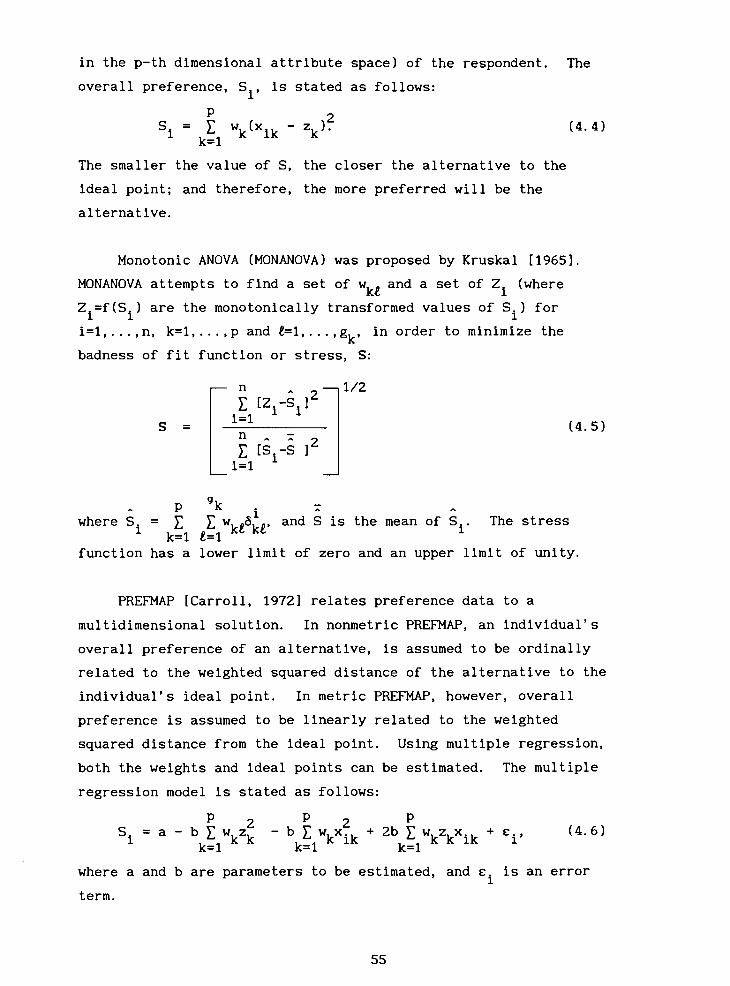
in the p-th dimensional attribute space) of the respondent. The

overall preference, Si, is stated as follows:

The smaller the value of S, the closer the alternative to the

ideal point; and therefore, the more preferred will be the

alternative.

Monotonic ANOVA (MONANOVA) was proposed by Kruskal 119651.

MONANOVA attempts to find a set of wke and a set of Z (where i

Z.=f(S.) are the monotonically transformed values of Si) for 1 1

i=l, . . . , n, k=l, . . . , p and e=l,. . . ,gk, in order to minimize the badness of fit function or stress, S:

where Si = 1 ~ ~ ~ 6 ; ~ . and S is the mean of Si. The stress k=l e=i

function has a lower limit of zero and an upper limit of unity.

PREFMAP [Carroll, 19721 relates preference data to a

multidimensional solution. In nonmetric PREFMAP, an individual's

overall preference of an alternative, is assumed to be ordinally

related to the weighted squared distance of the alternative to the

individual's ideal point. In metric PREFMAP, however, overall

preference is assumed to be linearly related to the weighted

squared distance from the ideal point. Using multiple regression,

both the weights and ideal points can be estimated. The multiple

regression model is stated as follows:

where a and b are parameters to be estimated, and E is an error i term.

Srinivasan and Shocker 119731 developed a linear programming

model (LINMAP) in preference decomposition. Let R = {(i,j)) be

the set of all paired comparisons obtained from the respondent

with the i-th alternative being more preferred to the j-th

alternative. Using the part worth function model as the

preference function, their model is stated as follows:

MIN dij (i, ~)ER

w is the estimated value of the part worth f (x for kt k kt k=1,2,. . . ,p and l=1,2,. . . , gk'

(LINMAP) is designed for ordinally-scaled preference data.

When ordinally-scaled preference data is collected by paired

comparison approach, the respondent is asked to state which

alternative is more preferred. However, more information may be

contained in ratio-scaled preference data when the respondent is

asked to state how many times the preferred alternative is being

more preferred to the other alternative. Since (LINMAP) does not

incorporate the higher level preference information when

estimating the part worth, I develop a linear programming model

which utilizes ratio-scaled preferences judgments as the input

data.

4.3 MODEL FORMULATION

In this section, I introduce a linear goal programming model

for preference decomposition (GPD), with the input preference

judgments measured in ratio scale. Let the overall preference

associated to the i-th alternative be quantified by S i'

i=1,2, ..., n, and for each pair of alternatives i and j, the i-th alternative is preferred to the j-th alternative whenever S >S

i J' Let R = {(i,j,t 1) be the set of all paired comparisons obtained

i .I from the respondent, with the i-th alternative being t times

i j more preferred to the j-th alternative for tijrl. Then for each

i t in R, we expect the ratio (S /S 1 to be t under i j i J i j

perfect consistency. That is,

- t S = 0 , i j j V(i, j, t 1 in R. i j

To be consistent with the input preference structure (4.10) in R,

it is desirable that

i=1,2,. . . ,n, satisfy

A

the estimated overall preferences Si,

in (4.11) is too restrictive, deviational Since exact equality +

variables d and dij are introduced to allow for inconsistencies i j which may exist in the input preference structure in R. Thus

(4.11) becomes

+ - C

+ The sum (dij + dij) of all dij and dij in (4.12) is

(i, j, tij)cR A

the badness of fit between Si and S with respect to the input i

preference structure in R. Substituting (4.1) into (4.121, we get

V , , t i j in . Thus the problem of finding the best solution

{wkL) from the data matrix X and the input preference R reduces to

a goal programming problem of finding {wke) which minimizes the + - -~ ~

badness of fit C (dij + dij) subject to the (i, j, tij)~R

constraints (4. l3), V (i, j,t ) in R. i j

However, it is sometimes difficult for the respondent to

express the exact value of t directly. It is better to ask the i j respondent "at least" how many times he/she prefers the i-th

alternative to the j-th alternative instead of asking hidher the

exact number of times he/she prefers the i-th alternative to the

j-th alternative. Intuitively this allows more robust input from

the respondent and hence more reliable results may be obtained

from the goal programming model. Now suppose Q = {(i,j,t 1) is i J

the set of all paired comparisons obtained from the respondent

with the i-th alternative being at least t times more preferred i j

to the j-th alternative. Then for each (i, j, ti , I , the positive + A ,. A .J

value of d- ij (dij

=0) implies that Si<tijSj, which conflicts

directly with the input preference in 52. But the positive value

of dlj (d: .=O) implies that ii>tijSj, which is still consistent 13 -

with the input preference in 52. Consequently, d i i should be + J

minimized before dij is minimized in the objective function.

I can now define formally the goal programming model for the

preference decomposition as follows:

(GPD) MIN P1 [ (i, j, C I J t. .)EQ d;j]+~2[ (i, j, i tij)€Q d;j] (4.141

P is much greater than P to allow for a larger penalty on the 1 2

+ deviational variables d- than di j.

i j Perhaps (GPD) should be

solved as a preemptive goal programming problem [Kornbluth, 19731 +

so that no part of d is ever traded off by any part of d- ij'

The i J -

primary objective is to minimize C di j in attempting

i j t )EQ i j

S The secondary objective is to minimize to achieve Sirtij j.

+ A A

C di j for reaching S i =t ij S j' (i, j, t. .)dl

1 J

P The inequity 1

k= 1

constraint. It can be

relative values of the

same if the right hand

1 wke L 1 is the normalization e=i

shown by direct verifications that the

optimal part worths wkt will remain the

side of the normalization constraint is

changed to any positive constant other than 1. Furthermore, for

any nontrivial solution {wit) which is feasible in (GPD) without

the normalization constraint, there exists a feasible solution

{w;} in (GPD) such that the relative values of w are the same

as the corresponding relative values of {w" ). Thus, the only kt effect of the normalization constraint in (GPD) is to avoid the

trivial solution (all wkfO).

The wkt obtained from solving (GPD) can then be used to

compute the estimated preference for any alternative by simply

summing up w for all relevant part worths. Thus the rank kt ordering of all the alternatives can be determined by the

magnitudes of their estimated preferences.

4.3.1 Discussion

Several parameter estimation methods in preference

decomposition can be used to estimate the part worths. In

particular, linear programming techniques for multidimensional

analysis of preferences (LINMAP) have higher predictive validity

over other methods when there is a dominant attribute [Wittink and

Cattin, 19811. (LINMAP) posits that Si-s.10 whenever the i-th J

alternative is preferred to the j-th alternative. The overall

preference, Si, may also be defined in terms of the distance from

the i-th alternative to an ideal alternative. In (GPD), Si-SjzO

is replaced by Si/S It with tijtl. Conceptually, Si/S.rtij j ij J has more preference information than S.-S 10 when t >1.

1 J i j

Furthermore, the only feasible solution cut off by the

normalization constraint in (GPD) is the trivial solution. There

is no unnecessary restrictions introduced by the normalization

constraint.

Usually, it is easier for a respondent to identify the

preferred alternative as compared to express the magnitude of

hidher preference. The cost of having more preference

information in S /S rt is the difficulty in eliciting tij from i j iJ

the respondent. One possible method to determine t is the i j

constant sum pairwise comparisons by Torgerson [19581. Another

way to assist a respondent in determining tij in the paired

comparison is the nine points intensity scale used in the Analytic

Hierarchy Process [Saaty, 19771. Harker and Vargas [I9871

supported the use of the 1 to 9 scale in Saaty' Analytic Hierarchy

Process. The ratio scale used in the Analytic Hierarchy Process

ranges from 1 to 9 and represents the preference of one

alternative to the other such as:

1 - indifference: at least 1 time, 3 - slightly more preferred: at least 3 times, 5 - strongly more preferred: at least 5 times,

7 - demonstratedly more preferred: at least 7 times, 9 - absolutely more preferred: at least 9 times.

Intermediate values of 2,4,6 and 8 are used when a more refined

compromise is needed. As long as all the paired comparisons of a

respondent are underestimated in the 9 points scale, the

constraints S./S.rt implicitly implied by (4.15) in (GPD) are 1 J ij

accurate and thus the corresponding solutions are meaningful.

Theoretically, there are (gl)(g2) . . . (g distinct P

alternatives from which n of them are selected for preference

evaluation, and there are n(n-1)/2 distinct pairwise comparisons.

When n is large, it is not feasible to conduct all the paired

comparisons. Thus the set R used in (GPD) may be replaced by a

well selected subset R' of R. In practice, only the paired

comparisons in R' would be elicited from the respondent and

incorporated into (GPD). Orthogonal array is one of the many

methods available for the selection of some representative subset

R' from R [Green, 19741. Table 4.1 illustrates an orthogonal

array of four attributes, each with three levels. It should be

pointed out that more reliable solutions would be obtained from

(GPD) by increasing the size of the subset R'.

Table 4.1: A Symmetrical Orthogonal Array for the 4 3 Factorial Design

- --

Attributes and Levels

Alternative

4.3.2 Computation Example

Consider the preference of alternatives with four attributes,

each with three levels of values. By using orthogonal arrays,

nine alternatives are selected to be included in the development

sample with the remaining 72 alternatives in the validation

sample. To test whether (GPD) can perform well and predict

preferences from other models, the input preference is generated

by the vector model (4.2). The attribute values yke for the nine

chosen alternatives X, the weights wk for the four attributes W

and the overall preferences Si of the alternatives XW are:

A random error value, E is added to each of the nine overall i

preferences in XW. The random error has zero mean and a constant

variance. The perturbed values of the nine overall preferences

XW+E are used as input into (GPD). The part-worth values w k.!? obtained from solving (GPD) and the original attribute values yke

are given in Table 4.2 below:

Table 4.2: The Part-worth values wke obtained from (GPD) and the

original attribute values y k .!?

ATTRIBUTE

LEVEL 1 2 3 4 1 2 3 4

1 1 1 1 1 0.000 0.000 0.088 0.079 2 2 3 2 2 0.011 0.025 0.065 0.129 3 3 5 4 10 0.041 0.065 0.141 0.356

The estimated part-worth values w are used to compute the A k.!?

estimated overall preference Si for the nine alternatives in the

development sample and the 72 alternatives in the validation

sample. The predictive validity is supported by the Pearson

correlation coefficient of 0.942 and the Spearman rank coefficient A

of 0.944 between the original Si values and the estimated Si

values in the validation sample. The Pearson correlation

coefficient and the Spearman rank coefficient between the original A

S. values and the estimated Si values in the development sample 1

are 0.942 and 0.883 respectively. (GPD) has performed well in

this example.

4.4 SIMULATION EXPERIMENT

I design a simulation experiment to evaluate the performance

of (GPD), (LINMAP) and Ordinary Least Squares (OLS) approaches in

preference decomposition. The data generation procedure is

similar to Wittink and Cattin [19811. The input preference Si is

derived from the part-worth function model, equation (4.1 1, where

all the part worths are drawn from a normal distribution with mean

zero and variance one. In this experiment, 30 data sets are used,

each data set consisting of 81 alternatives with four attributes,

each having three levels of values or part worths. By using

orthogonal arrays, nine alternatives are selected to be included

in the development sample with the remaining 72 alternatives in

the validation sample. A random error value is added to each of

the nine overall preferences in the development sample. The

random error has zero mean and its variance a2 is computed from e the same formula used by Wittink and Cattin as follows:

2 where 13~ is the error variance and 6 is the variance in the

e s overall preference S before the error term is introduced. I use i three different values, 0.1, 0.2, and 0.35 for E in this

experiment. The higher the value of E, the larger is the noise

term being introduced into the input preference. I randomly

generated 10 data sets for each of the E values, and the perturbed

values of the nine overall preferences are used as input into

(GPD), (LINMAP), and (OLS). The softwares I used for (LINMAP) and

(OLS) are Conjoint Linmap [19891, and Conjoint Analyzer [ 19871,

respectively.

The estimated part-worth values w obtained from the models kt ,. are used to compute the estimated overall preference S for the 72 i alternatives in the validation sample. The predictive validity is

evaluated by the average Pearson correlation coefficient and the

average Spearman rank coefficient between the original S values i

A

and the estimated S values in the validation samples. The i

results are reported in Table 4.3.

Table 4.3: Average Pearson correlation coefficient and average Spearman rank coefficient of (CPD), LINMAP and (OLS)

Pearson correlation Spearman rank coefficient coefficient

E (GPD) (LINMAP) (OLS) ( GPD 1 (LINMAP) (OLS)

average 0.910 0.857 0.911 0.904 0.860 0.903

The average Pearson correlation coefficient and the average

Spearman rank coefficient of (GPD) and (OLS) are higher than the

coefficients of (LINMAP) in all three cases. For the Pearson

correlation coefficient, (GPD) is higher than (LINMAP) by 0.0541,

0.0522, and 0,0492 when E equals to 0.1, 0.2, and 0.35,

respectively. For the Spearman rank coefficient, (GPD) is higher

than (LINMAP) by 0.0451, 0.0511, and 0.0368 when E equals to 0.1,

0.2, and 0.35, respectively. In all three cases, both the average

Pearson correlation coefficients and the average Spearman rank

coefficients of (GPD) and (OLS) are very close to each other.

4.5 CONCLUSION

A linear goal programming model (GPD) is introduced to

estimate the part worths in preference decomposition. The model

uses ratio scaled input preference judgments which contain more

preference information than ordinal scaled preference judgments

commonly used in many preference decomposition models. Since the

objective of (GPD) is to directly minimize the badness of fit

between the input preferences and the derived preferences, more

reliable estimates for the part worths may be expected from the

model. In this simulated experiment (GPD) and (OLS) have better

performance than (LINMAP) in terms of the Pearson correlation

coefficient and the Spearman rank coefficient between the input

preference and the derived preference. Additional empirical

studies are needed to evaluate the efficiency and the predictive

power of (GPD).

CHAPTER 5

CONCLUSION

In this paper, I develop several new linear goal programming

models to solve the problems in classification and preference

decomposition. In chapter 2, with an analog of multicriteria

optimization framework, I provide a systematic way of generating a

whole array of meaningful criteria and introduce five new

mathematical programming models for cluster analysis. The ability

to generate many meaningful criteria for evaluating cluster

solutions increases the power and the flexibility of applying

mathematical programming approaches to cluster analysis. This

will likely motivate more frequent applications of mathematical

programming approaches to cluster analysis. The computational

results obtained from applying the clustering models to a

published data set support the use of mathematical programming

models. Future researches applying the above techniques to

solve the problems in cluster analysis should be very interesting.

In chapter 3, I introduce two new linear goal programming

models for discriminant analysis. The model (GP1) incorporates

the within group discriminate information in discriminant

analysis. It is based on the order preservation of selected pairs

of membership probabilities in the development sample.

Intuitively, this model may provide more accurate estimations of

the attribute weights than other techniques which ignore the

within group discriminate information. It has good performance

in both the M.B.A. admission problem and the simulation

experiment. The model (GP2) allows non-monotonic attributes to be

included in the classification function. Since in some

situations, the implied monotonicity of the attribute scores may

be violated, thus (GP2) provides more flexibility in applying

linear programming techniques to classification problems. The

results from the simulation experiment support the use of (GP2) to

solve the classification problems when non-monotonic attributes

are present.

The existing linear programming approaches in preference

decomposition only allow the input preference judgments to be

measured in ordinal scale. Theoretically, ratio scale preference

judgments contain more information than ordinal scale preference

judgments. Therefore, in chapter 4, I introduce a linear goal

programming model (GPD) for preference decomposition with the

input preference judgments measured in ratio scale. (GPD)

performs well in the simulation experiment. Although the

performance of (GPD) and (OLS) are close in the simulation

experiment, (GPD) has the advantage that additional constraints

which reflect useful prior information can easily be added.

REFERENCES

Anderson, J.A. (1972) "Separate Sample Logistic Discrimination", Biometrika, 59, 19-35.

Aronson, J.E., and Klein, G. (1989) "A Clustering Algorithm for Computer-Assisted Process Organization," Decision Sciences 20, 730-746.

Arthanari, T.S., and Dodge, Y. (1981) Mathematical Programming in Statistics. Wiley, NY.

Bajgier, S. M. , and Hill, A. V. (1982) "An Experimental Comparison of Statistical and Linear Programming Approaches to the Discriminant Problem", Decision Sciences 13, 604-618.

Blashf ield, R. K. and Aldenderfer, M. S. (1978) "The Literature on Cluster Analysis," Multivariate Behavioral Research 13, 271-295.

Carroll, J.D. (1972) "Individual Differences and Multidimensional Scaling", Multidimensional Scaling: Theory and Applications in Behavioral Sciences, Vol. I , R. N. Shepard et al. , eds. Seminar Press, New York, 105-155.

Chankong, V. and Haimes, Y.Y. (1983) "Optimization-Based Methods for Multiobjective Decision-Making: An Overview", Large scale System 5, 1-33.

Charnes, A. , Cooper, W. W. , and Ferguson, R. 0. (1955) "Optimal Estimation of Executive Compensation by Linear Programming", Management Sciences 1, 138-150.

Choo E. U. , and Wedley, W. C. (19851, "Optimal Criterion Weights in Repetitive Multicriteria Decision Making", Journal of Operational Research Society 36, 983-992.

Church, R. , Current, J. , and Storbeck, J. (1991 1 " A Bicriterion Maximal Covering Location Formulation Which Considers the Satisfaction of Uncovered Demand," Decision Sciences 22, 38-52.

Conjoint Analyzer (19871, Software, Bretton-Clark, Morristown, NJ 07960.

Conjoint Linmap (1989), Software, Bretton-Clark, Morristown, NJ 07960.

Cox, D.R. (1970) The Analysis of Binary Data. London: Methuen.

Day, N.E. and Kerridge, D.F. (1967) "A General Maximum Likelihood Discriminant", Biornetrics 23, 313-328.

Fisher, R.A. (1936) "The Use of Multiple Measurements in Taxonomic Problems", Annals of Eugenics 7, 179-188.

Flath, D. and Leonard, E.W. (1979) "A Comparison of Two Logit Models in the Analysis of Quantitative Marketing Data", Journal of Marketing Research 16, 533-538.

Freed, N. and Glover, F. (1981a) "A Linear Programming Approach to the Discriminant Problem", Decision Sciences 12, 68-74.

Freed, N. and Glover, F. (1981b) "Simple but Powerful Goal Programming Models for Discriminant Problems", European Journal of Operational Research 7, 44-60.

Freed, N., and Glover, F. (1986) "Evaluating Alternative Linear Programming Models to Solve The Two-Group Discriminant Problem", Decision Sciences 17, 151-162.

Ghosh, A. and Craig, C. S. (1986) "An Approach to Determining Optimal Locations for New Services," Journal of Marketing Research 23, 354-62.

Glover, F. , Keene, S., and Duea, B. (1988) "A New Class of Models for the Discr'iminant Problem", Decision Sciences 19, 269-280.

Gordon, A. D. (1981 1 Classification, New York: Wiley.

Green, P.E. (1974) "On the Design of Choice Experiments Involving Multi-factor Alternatives", Journal of Consumer Research 1, 66 1-678.

Green, P. E. and Rao, V.R. (1971) "Conjoint Measurement for Quantifying Judgmental Data", Journal of Marketing Research 8, 355-363.

Green, P. E. and Srinivasan, V. (1978) "Conjoint Analysis in Consumer Research: Issues and Outlook", Journal of Consumer Research, 5, 103-123.

Hand, D.J. (1981) Discrimination and Classification. New York: Wiley.

Harker, P. T. and Vargas, L. G. (1987) "The Theory of Ratio Scale Estimation: Saaty's Analytic Hierarchy Process", Management Sciences, 33, 1383- 1403.

Joachimsthaler, E.A., and Stam, A. (1988) "Four Approaches to the Classification Problem in Discriminant Analysis: An Experimental Study", Decision Sciences 19, 322-333.

Johnson, R. A. and Wichern, D. W, (1988) Applied Mu1 tivariate Statistical Analysis, 2nd Edition, New Jersey:Prentice Hall.

Johnson M.E. (1987) "Multivariate Statistical Simulation", John Wiley and Sons.

Johnston, J. (1972) Econometrics Methods, 2nd edition, New York, McGraw-Hill Book Co.

Koehler, G. J. and Erenguc, S.S. (1990) "Minimizing Misclassifications in Linear Discriminant Analysis", Decision Sciences 21, 63-85.

Kornbluth J. (1973) "A Survey of Goal Programming", OMEGA 1, 193-205.

Kruskal, J.B. (1965) "Analysis of Factorial Experiments by Estimating Monotone Transformations of the Data", Journal of the Royal Statistical Society, Series B, 27, 251-263.

Lee, C. K. and Ord, J. K. (1990) "Discriminant Analysis Using Least Absolute Deviations", Decision Sciences 21, 86-96.

MacQueen, J.B. (1967) "Some Methods for Classification and Analysis of Multivariate Observation," Proceeding of 5th Berkeley Symposium on Mathematical Statistics and Probability, 1, Berkeley, Calif. : University of California Press, 281-97.

Milligan, G. W. and Cooper, M. C. (1985) "An Examination of Procedures for Determining the Number of Clusters in a Data Set," Psychometrika 50, NO. 1, 159-179.

Ragsdale, C., and Stam, A. (1989) "A Robust Nonparametric Procedure to Estimate Response Functions for Binary Choice Models", presented at the CORS/TIMS/ORSA 1989 Conference, Vancouver, Canada.

Rao, M.R. (1971) "Cluster Analysis and Mathematical Programming," Journal of the American Statistical Associations 66, 622-626.

Revelle, C., Marks, D. and Liebman, J.C. (1970) "An Analysis of Private and Public Sector Location Models," Management Science 16, 692-707.

Saaty, T.L. (1977) "A Scaling Method for Priorities in Hierarchical Structures", Journal of Mathematical Psychology 15, 234-281.

SPSS Inc. (1988) SPSS-X User9 s Guide, 3rd ed. , SPSS Inc.

Srinivasan, V., Jain, A, and Malhotra, N.K. (1983) " Improving Predictive Power of Conjoint Analysis by Constrained Parameter Estimation", Journal of Marketing Research 20, 1983, 433-438.

Srinivasan, V. (1975) "Linear Programming Computational Procedures for Ordinal Regression", Journal of the Association for Computing Machinery 23, 475-487.

Srinivasan, V. and Shocker, A. D. (1973) "Linear Programming Techniques for Multidimensional Analysis of Preferences", Psychomet rika 38, 337-69.

Stam, A. and Joachimsthaler, E.A. (1989) "Solving the Classification problem in discriminant analysis via linear and nonlinear programming methods", Decision Sciences, 20, 285-293.

Stam, A. and Joachimsthaler, E. A. (1990) "A Comparison of a Robust Mixed-integer Approach to Existing Methods for Establishing Classification Rules for the Discriminant Problem", European Journal of Operational Research, 46, 113-122.

Stam, A. and Ragsdale, C. T. (1990) "A Robust Nonparametric Procedure to Estimate.Response Functions for Binary Choice Models", Operations Research Letters, 9, 51-58.

Stam, A. and Jones, D. G. (1990) "Classification Performance of Mathematical Programming Techniques in Discriminant Analysis: Results for Small and Medium Sample Sizes", Managerial and Decision Economics, 11. 243-253.

Torgerson, W.S. (1958) Theory and Methods of Scaling, New York, John Wiley & Sons Inc.

Vinod, H.D. (1969) "Integer Programming and Theory of Grouping," Journal of the American Statistical Association 64, 506-519.

Wagner, H.M. (1959) "Linear Programming Techniques for Regression Analysis", Journal of the American Statistical Association 54, 206-212.

Wittink, D. R. and Cattin, P. (1981 "Alternative Estimation Methods for Conjoint Analysis: A Monte Carlo Study", Journal of Marketing Research 18, 101-106.