Linear and non-linear deformations of a wind turbine blade ...

Wayne State University

Wayne State University Dissertations

1-1-2012

Linear and non-linear deformations of a windturbine blade considering warping and allaeroelastic load couplingsFouad Mohammad MohammadWayne State University,

Follow this and additional works at: http://digitalcommons.wayne.edu/oa_dissertations

Part of the Mechanical Engineering Commons, and the Oil, Gas, and Energy Commons

This Open Access Dissertation is brought to you for free and open access by DigitalCommons@WayneState. It has been accepted for inclusion inWayne State University Dissertations by an authorized administrator of DigitalCommons@WayneState.

Recommended CitationMohammad, Fouad Mohammad, "Linear and non-linear deformations of a wind turbine blade considering warping and all aeroelasticload couplings" (2012). Wayne State University Dissertations. Paper 463.

http://digitalcommons.wayne.edu/?utm_source=digitalcommons.wayne.edu%2Foa_dissertations%2F463&utm_medium=PDF&utm_campaign=PDFCoverPages

http://digitalcommons.wayne.edu/?utm_source=digitalcommons.wayne.edu%2Foa_dissertations%2F463&utm_medium=PDF&utm_campaign=PDFCoverPages

http://digitalcommons.wayne.edu/oa_dissertations?utm_source=digitalcommons.wayne.edu%2Foa_dissertations%2F463&utm_medium=PDF&utm_campaign=PDFCoverPages

http://digitalcommons.wayne.edu/oa_dissertations?utm_source=digitalcommons.wayne.edu%2Foa_dissertations%2F463&utm_medium=PDF&utm_campaign=PDFCoverPages

http://network.bepress.com/hgg/discipline/293?utm_source=digitalcommons.wayne.edu%2Foa_dissertations%2F463&utm_medium=PDF&utm_campaign=PDFCoverPages

http://network.bepress.com/hgg/discipline/171?utm_source=digitalcommons.wayne.edu%2Foa_dissertations%2F463&utm_medium=PDF&utm_campaign=PDFCoverPages

http://digitalcommons.wayne.edu/oa_dissertations/463?utm_source=digitalcommons.wayne.edu%2Foa_dissertations%2F463&utm_medium=PDF&utm_campaign=PDFCoverPages

LINEAR AND NON-LINEAR DEFORMATIONS OF A WIND TURBIN E BLADE CONSIDERING WARPING AND ALL AEROELASTIC LOAD COUPLINGS

by

FOUAD MOHAMMAD MOHAMMAD

DISSERTATION

Submitted to the Graduate School

of Wayne State University,

Detroit, Michigan

in partial fulfillment of the requirements

for the degree of

DOCTOR OF PHILOSOPHY

2012

MAJOR: MECHANICAL ENGINEERING

Approved by

__ Advisor Date

___________________________________

_____

© COPYRIGHT BY


2012

All Rights Reserved

ii

DEDICATION

Dedicated to

GOD

(The Reason of Everything)

then to

… my parents,

my wife & my kids,

my country: Canada,

my motherland: Palestine,

& in loving memory of my grandparents

iii

ACKNOWLEDGEMENTS I would like to express my deepest gratitude to my professor, Dr. Emmanuel

Ayorinde, without whom this work would not be possible, for giving me this opportunity, for all

his teachings, his insight, warm advice and guidance.

I thank the members of my PhD dissertation committee: Prof. Xin Wu, Prof. Tawfik

Khalil and Prof. Hwai-Chung Wu for their guidance and suggestions. I also thank Prof.

Trilochan Singh for all his advice and support.

I am grateful to all my students of the ME-7020 class for their encouragement and to

all my friends at Wayne State University for being the surrogate family during the many years I

stayed there. To mention few: from the department staff: Ms. Stephanie A. Sepko and Ms.

Rosalind Willis and from the engineering library: Ms Sherry Barclay.

Special thanks go to Prof. Ronald M Barron at University of Windsor for answering

my questions on some numerical iteration schemes, to Dr. Alan Wright at NREL for directing

me to many great wind turbine references and to Mr. Marshall L. Buhl Jr. at NREL for

answering my questions on some NREL wind turbine codes such as FAST and Precomp.

Finally, I am forever indebted to: My parents (Jawhara Mansour and Mohammad

Mohammad) for their endless encouragement. My wife (Nariman Al-Attal) for her endless care

and support- at all times. My kids (Mohammad, Jawhara, Zakareya and Taha) for their

endless patience when it was most needed.

iv

PREFACE

A wind turbine blade similar to a helicopter rotor blade has the structure of a pretwisted beam

of a variable airfoil asymmetrical cross-section. A number of approximate theories have been

developed by different researchers to study the dynamic behavior of the blade of a horizontal

axis wind turbine that reacts due to axial, torsional and flexural aerodynamic loadings and to

the coupling interactions among all of these loadings. The new contribution in this present

research is the consideration of all the extensional, torsional and flexural loadings with their

couplings, variable airfoil cross sections with warping effects, shear deflection, rotary inertia

and with or without blade’s pretwist for both the linear small deformation case and the

nonlinear large deformation case. To the best knowledge of the author the simultaneous

inclusion of all these factors has not been done before. The mass matrix, linear and nonlinear

stiffness matrices and the load vector (function of time step) of the dynamic equations of

motion are deduced from the Lagrange equations of motion that were derived step by step.

The steps of the linear and nonlinear Newmark implicit iteration schemes used for solving the

dynamic equations of motion respectively were explained in detail. Numerical implementation

examples for both linear and nonlinear cases were demonstrated for a 14m long blade with

and without pretwisting that has specific material and geometrical properties and a decreasing

NACA4415 airfoil cross section from hub to tip. For both of the linear and nonlinear examples,

the aerodynamic loadings (lift, drag and pitch moment) and the nonlinear stiffness matrices

were computed at each time step utilizing a time dependent set of parameters such as angle of

attack, material and air density, wind and blade speed, flow angle, yaw and pitch angles.

Then the unknown displacements , and in the directions of x, y and z axes respectively,

the bending rotations and about the y and z axes respectively and the torsional rotation

about the x axis, were solved using the linear and nonlinear Newmark implicit iteration

schemes.

v

TABLE OF CONTENTS

Dedication…………………………………………………………………………………………...ii

Acknowledgements………………………………………………………………………………..iii

Preface……………………………………………………………………………………………...iv

List of Tables……………………………………………………………………………………….ix

List of Figures & Charts……………………………………………………………………………x

Notations Used……………………………………………………………………………………xiii

Chapter 1: Literature Review on Blade Design & Research Objectives

1.1 Introduction………………………………………………………………………………....1

1.2 Structural Layout Design and Aerodynamic Loads…………………………………….2

1.2.1 Design Factors……………………………………………………………………..2

1.2.2 Structural Design…………………………………………………………………..8

1.2.3 Barriers in Scaling up Conventional Blade Designs……………………….....11

1.2.4 Blade Lift, Drag, Pitch Moment and Stall Phenomena ……………………....12

1.2.5 Wind Turbine Blade Materials…………………………………………………...15

1.2.5.1 Different Blades Composites Manufacturing Processes………..........16

1.2.5.2 The Fiber Alignment in Fiber Carbon……………………………………19

1.2.6 Varying Properties along the Blade……………………………………………..20

1.3 Research Motivation and Objectives…………………………………………………...23

1.3.1 Research Motivation……………………………………………………………..23

1.3.2 Research Objectives…………………………………………………………….24

1.4 Aerodynamics Loads………………………………………………………………….....26

1.4.1 Airfoil’s load Layout………………………………………………………………26

1.4.2 Simple Load Formulas / Model ………………………………………………...27

vi

1.5 Blade Element Momentum Theory …………………………………………………….30

Chapter 2: Literature Review on Blade Different Formulations & Research Plan

2.1 Introduction………………………………………………………………………………..42 2.2 Aeroelasticity………………………………………………………………………….......43 2.3 Large Deformation versus Small Deformation……………………….………………..45

2.4 Aeroelastic Coupling Schemes…………………………………...…………………….46

2.5 Optimization of Blade Design…………………………………...………………………48

2.6 Finite Element Beam Formulation…………………………...………………………….49

2.7 Non-linearity due to large Deformation……………...………………………………....53

2.8 Research Tasks and Plan …………………………...……………………………….....54

2.8.1 Lagrangian Beam Formulation…………………………………………….........54

2.8.2 Model Validation……………………………………………...............................55

2.8.2.1 Experimental Testing ………………………………………………………55 2.8.2.2 Blade Analysis Using Hypermesh and Ls-Dyna……………………......56 2.9 Torsion of Arbitrary Cross-sections ………………...…………………………………..63

2.9.1 Saint-Venant’s Torsion Theory…………………………………………………..63 2.9.2 Prandtl Stress Function Theory………………………………….......................67 2.9.3 Cross-section Geometrical Properties…………………………………………..71

2.9.3.1 Torsional Rigidity Calculation………………………………………….....71

2.9.3.2 Second Moment of Inertia …………………………………………..........71

2.9.3.3 Product Moment of Inertia…………………………………………...........72

2.9.3.4 Polar Moment of Inertia…………………………………………...............73

Chapter 3: Total Strain Energy, Total Kinetic Energy, Aerodynamic loadings & External Work

3.1 Introduction…………………………………………………………………………...........75

vii

3.2 Dynamic Equations of Motion…………………………………………………..............76

3.3 Computation of the Total Strain Energy ……………………………………................78

3.4 Computation of the Total Kinetic Energy ………………………………………………78

3.5 Displacement Expansion…………………………………………………………..........79

3.6 Thrusts, Torques, Centrifugal Forces and Pitch Moments…………………………...80

3.7 External Work……………………………………………………………………………..82

3.8 Boundary Conditions……………………………………………………………………..83

Chapter 4: Obtaining the Lagrange Equations of Motion

4.1 Introduction………………………………………………………………………………...85

4.2 Derivation of the Lagrange Equations of Motion………………………………..........87

Chapter 5: Arranging the Mass, Linear & Non-linear Stiffness Matrices

5.1 Introduction…………………………………………………………………………...........94

5.2 Arranging the Linear Mass and Stiffness Matrices…………………………………….94

5.3 Arranging the Non-linear Stiffness Matrices…………………………………………....98

Chapter 6: Displacements Solution Using the Newmark Implicit Procedure

6.1 Introduction…………………………………………………………………………….....106

6.2 Implicit Dynamics versus Explicit Dynamics Schemes……………………………...107

6.3 The Linear Implicit Newmark Methods………………………………………………...108

6.4 The Linear Implicit Newmark Iteration Procedure Steps…………………………….112

6.5 Stability Conditions for the Newmark Methods………………………………………113

6.6 The Non-linear Implicit Newmark Iteration Procedure Steps……………………….115

Chapter 7: The Selected Blade Design

7.1 Introduction ………………………………………………………………………………118

7.2 Rotor Specifications and Dimensions …………………………………………………119

7.3 Angle of Attack ………………………………………………………………………….120

viii

7.4 Airfoil Profile Properties…………………………………………………………………123 7.4.1 NACA-4415 Airfoil Profile Properties ………………………………….………124 7.4.2 S809 Airfoil Profile Properties…………………………………………………..128 7.5 Blade Different Airfoil Geometrical Properties………………………………………..133 7.6 Calculation Procedure of the R-Load Vector at Each Airfoil Station for Every Time Step………………………………………………………………………………………...136 Chapter 8: Implementation & Numerical Results 8.1 Introduction ……………………………………………………………………………….140

8.2 Numerical Application and Results……………………………………………….........141

8.2.1 Linear Small Deformation Case Example……………………………………..141

8.2.2 Non-linear Large Deformation Case Example………………………………..144

Chapter 9: Conclusion & Related Future Work

9.1 Conclusion ………………………………………………………………………………..149

9.2 Related Future Work …………………………………………………………………….151

Appendix A………………………………………………………………………………………….152

Appendix B………………………………………………………………………………………….155

Appendix C………………………………………………………………………………………….157

Appendix D………………………………………………………………………………………….164

Table A ……………………………………………………………………………………………..167

Table B ……………………………………………………………………………………………..169

References …………………………………………………………………….............................172

Abstract……………………………………………………………………………………………...180

Autobiographical Statement ……………………………………………………………………...182

ix

LIST OF TABLES

Table1.2.5.1.1: The Comparison between Prepreg, Infusion and RTM……………19

Table 1.5.1: The Number of Blades…………………………………………………..40

Table 6.5.1: Properties of the Members of the Newmark Family of Methods….115

Table 7.4.1.1: NACA-4415 Airfoil Coordinates……………………………………....124

Table 7.4.1.2: Cl, Cd and Cm w.r.t. alpha for NACA-4415 Airfoil…………………..126

Table 7.4.2.1: Coordinates of S809 Airfoil Profile…………………………………....128

Table 7.4.2.2: Cl, Cd and Cm w.r.t. Angle of Attack for S809 Airfoil……………….130

Table 7.5.1:

Table 7.5.2:

Blade Stations Airfoil Profile Properties……………………………...134

Wind Properties…………………………………………………………135

Table 7.5.3: Table 7.6.1.1: Table 8.2.1.1: Table 8.2.2.1: Table A: Table B:

Angle of Attack Values at all Considered Stations………………….136 Aerodynamic Forces and Moments at Different Stations in and about x, y and z directions…………………………………………………….137 Blade Properties for the Linear Example…………………………….141

Blade Properties for the Non-linear Example………………………..145

Values of D’s as Function of x…………………………………….......167

All S Integral Definitions………………………………………………..169

x

LIST OF FIGURES & CHARTS

Fig. 1.1.1: The Wind Turbine Growth ............................................................ ….1

Fig. 1.2.1.1: The Wind Turbine Airfoil .............................................................. ….3

Fig. 1.2.1.2: Wind Turbine Blade Tip-Speed Ratio......................................... …..4

Fig. 1.2.1.3: Power Coefficient versus Tip-Speed Ratio .................................. ….4

Fig. 1.2.1.4: The Wind Turbine Efficiency ........................................................ ….5

Fig. 1.2.1.5: The Betz Criterion ........................................................................ ….5

Fig. 1.2.2.1: The Wind Turbine Blade Components………………………………...9

Fig. 1.2.2.2: The Wind Turbine Blade Airfoil Section……………………………...10

Fig. 1.2.2.3: The Different Blade Design Concepts ......................................... …11

Fig. 1.2.4.1: The Lift and Drag Forces ............................................................ …13

Fig. 1.2.4.2:

Fig. 1.2.4.3:

Fig.1.2.5.1.1:

The Flow Around an Airfoil .......................................................... …14

The Variation of the Angle of Attack at Hub and Tip .................. ….15

Composite Materials ................................................................. ….16

Fig.1.2.5.1.2: The Typical Wind Turbine Blade Structural Layout………………..17

Fig.1.2.5.2.1: Stitched Unidirectional Carbon Fabric with Induced Waviness…..20

Fig. 1.2.6.1: The Fiber Direction in a Composite Build of Unidirectional, Continuous Fibers ....................................................................... …22

Fig.1.4.1.1: The Local Forces on the Blade ................................................... ...27

Fig.1.4.2.1: The Wind and Force Vectors Acting on an Airfoil ..................... …29

Fig.1.5.1: Axial Stream Tube Around a Wind Turbine ................................. …30

Fig.1.5.2: Rotating Annular Stream Tube ................................................... …32

Fig.1.5.3: Rotating Annular Stream Tube Notation ..................................... …33

xi

Fig.1.5.4:

Fig.1.5.5:

Fig.1.5.6:

Fig.2.1.1:

Fig.2.2.1:

Fig.2.6.1:

Fig.2.6.2:

Fig.2.8.2.2.1:

Fig.2.8.2.2.2:

Fig.2.8.2.2.3:

Fig.2.8.2.2.4:

Fig.2.8.2.2.5:

Fig.2.8.2.2.6:

Fig.2.9.1.1:

Fig.2.9.3.4.1:

The Blade Different Stations ....................................................... .34

Flow onto the Turbine Blade ........................................................ .35

The Forces on the Turbine Blade ................................................ .36

Beam Element with Six Degrees of Freedom at Each Node..........42

Summary of Forces and Their Responses ................................... .44

Cantilever Beam with Two Degrees of Freedom at Each Node…..50

Six Degrees of Freedom .............................................................. .52

The Blade Stations ...................................................................... ..56

Airfoil Geometrical Properties Using Hypermesh ........................ …58

Changing 1D beams to a 3D Blade Using Hypermesh ................ .59

The Load Curves Data ................................................................ …60

The Final Blade Ls-Dyna Model .................................................. …61

All Stations Loadings .................................................................. …62

An Arbitrary Cross-section Under Torsion .................................. …65

The Polar Moment of Inertia ....................................................... …73

Fig. 3.2.1: Pre-twisted Asymmetrical Blade Structure Coordinate Systems.....76

Fig. 3.6.1: The Lift and Drag Forces ............................................................. ..81

Fig. 3.6.2: The Aerodynamic Loads .............................................................. ..82

Fig. 6.3.1 :

Chart 6.4.1:

Chart 6.6.1:

Fig. 7.2.1:

Newmark’s Constant-Average-Acceleration scheme ................... 109

Linear Newmark Procedure Flow Chart ....................................... 113

Non-linear Newmark Procedure Flow Chart ................................ 117

Three Blade Rotor Assembly ....................................................... 119

Fig.7.2.2: Blade Shape and Dimensions ...................................................... 120

Fig.7.3.1: Flow Around an Airfoil .................................................................. 121

xii

Fig. 7.3.2:

Fig. 7.4.1:

Fig. 7.4.1.1:

Chart7.4.1.1:

Chart7.4.1.2:

Chart7.4.1.3:

Fig. 7.4.2.1:

Chart7.4.2.1:

Chart7.4.2.2:

Chart7.4.2.3:

Fig 7.5.1:

Fig 7.5.2:

Fig 7.6.1.1:

Fig 8.2.1.1:

Fig. 8.2.1.2:

Fig 8.2.1.2:

Fig 8.2.1.3:

Fig 8.2.2.1:

Fig 8.2.2.2:

Fig. 8.2.2.3:

Fig. 8.2.2.4:

Fig. 8.2.2.5:

Fig. 8.2.2.6:

Velocity and Forces at a Blade Element at Radius r .................... 122

Airfoil Geometry ........................................................................... 123

Geometrical Shape of NACA-4415 Airfoil .................................... 125

Cl versus alpha for NACA-4415 ................................................... 127

Cd versus alpha for NACA-4415 .................................................. 127

Cm versus alpha for NACA-4415 ................................................. 128

Geometrical Shape of S809 Airfoil ............................................... 129

Cl versus alpha for S809 .............................................................. 131

Cd versus alpha for S809 ............................................................ 132

Cm versus alpha for S809 ........................................................... 132

Blade Different Airfoil Profiles ...................................................... 133

Angle of Attack versus Azimuth Angle ......................................... 135

Aerodynamic Forces and Moments ............................................. 137

Blade Geometry and Neutral Axis Line as Given by Younsi et al .142

Forces and Moments at all the Given 15 Stations ....................... 142

Blade Tip Linear Displacements and Rotations …………………...143

Comparison of Published Work With Present Work Results ... …..144

Nonlinear plots comparison for Tip Displacement in x-direction . .146

Nonlinear plots comparison for Tip Displacement in y-direction ..146

Nonlinear plots comparison for Tip Displacement in z-direction….147

Nonlinear plots comparison for Tip Rot. Displ. about x-direction...147

Nonlinear plots comparison for Tip Rot. Displ. about y-direction...148

Nonlinear plots comparison for Tip Rot. Displ. about z-direction…148

xiii

NOTATIONS USED

denotes differentiation with respect to time t

denotes differentiation with respect to x

mass per unit length and material density respectively

gravitational acceleration

area at any cross section and length of the beam respectively

effective Young’s and Shear Modulii at any cross section respectively

coordinate distance measured along the length of the blade from root

u bulk or logitudinal displacement on line of centre-of-flexure where y and z equal

to zero

longitudinal displacement of particles on the line of centroids

displacements in x, y and z directions respectively

displacement field

dynamic displacement of flexure centre & centroid respectively in yx plane

dynamic displacement of flexure centre & centroid respectively in zx plane

coordinate axes through centre of flexure and centroid respectively

; coordinates measured from centre of flexure and centroid respectively

second moment of area of cross section about and axes respectively

product moment of area of cross section about and axes respectively

polar mass moment of inertia per unit length about centre-of-flexure axis

or polar mass moment of inertia per unit length about centroid axis

distance between centre-of-flexure and centroid in direction respectively

)(•

)( ′

,m ρ

g

LA,

,E G

x

cu

wvu ,,

iu

1, yy

1,zz

,yy ;zz 1y ,1y 1z 1z

•y

•z

••11 zy

,yyI zzI 1y 1y 1z 1z

yzI 1y 1y 1z 1z

sI φ

φI αI

,αy αz zy,

xiv

beam pre-twisted angle

bending rotation about the axes (or in planes) respectively

blade pre-twist angle at

dynamic torsional deflection

stagger angle

rate of pre-twist assumed along the beam length

centroid center of mass axis ( loci of the mass centre of the cross section)

center of elasticity or flexure axis ( loci of the shear center of the cross section)

bending ( flexural) rigidities

coupled bending ( flexural) rigidity and torsional rigidity respectively

coupled flexure-torsional rigidities

cross section shear or shape correction factor and shear rigidity respectively

cross sectional warping and Prandtl stress function respectively

displacement of centroid in direction

ξξηη, coordinate axes through the centroid of the blade at root, tangential and normal

to the plane of disc rotation respectively

angular velocity

disc radius

etcR,

ext external

m,n,k,l integers that vary between 1 & M,N,K,L respectively

B.C. boundary condition

β

,1θ 2θ zy, zyzx,

β Lx =

φ

ς

K

C

O

,yyEI zzEI

,yzEI GJ

,1K 2K

,k kGA

,ψ ϕ

η η

ω

R

etcLR ,/

1

Chapter 1

Literature Review on Blade Design & Research Objectives

1.1 Introduction

The sizes of wind turbine mills have increased significantly over the last two decades [1], as

shown in Fig. 1.1.1, and will continue to do so in the coming few years to reach soon a rated

power output in the range of 8–10MW and a rotor diameter about 180 m. Nowadays, the

largest wind turbines have a rated power output of 5MW and rotor diameters of 126 m.

Fig. 1.1.1: The wind turbine growth [1].

The driving motivation behind this size increase is that larger wind turbines have larger

energy output per unit rotor area due to increased mean wind velocity with height. Moreover,

even though larger wind turbines are more expensive than smaller ones, the general trend is

that the total production cost per kilowatt hour of electricity produced decreases with increasing

2

wind turbine size. Present design methods and the available components and materials do not

allow up-scaling of wind turbine size as quoted by many designers, and to achieve the

necessary up-scaling, a need exists to address a number of areas that are considered critical

in achieving this, including innovative materials with a sufficient strength-to-mass ratio and

structural and material design of rotors. Among the materials used in wind turbine blades

manufacturing are polymer matrix composite materials, in a combination of monolithic (single

skin) and sandwich composites (a special type of composite laminate where two (or more) thin,

stiff, strong and relatively dense faces are separated by a thick, lightweight and compliant core

material. Such sandwich composites have gained widespread acceptance as an excellent way

to obtain extremely lightweight components and structures with very high bending stiffness,

high strength, and high buckling resistance. Glass fiber reinforced composites (GFRP) are in

use now, but for very large blades carbon fiber-reinforced composites have to be used, in

addition to GFRP, to reduce the weight.

1.2 Structural Layout Design and Aerodynamic Loads

1.2.1 Design Factors

Wind turbine mills that have between two and four aerodynamically efficient rotor blades give

better results than using many of them. Today’s mills have three-blade rotors which are now

the general trend. Similar to the wings of a plane, wind turbine blades use the airfoil shape to

create lift. As shown in Fig. 1.2.1.1, the lift force is perpendicular to the direction of the motion.

We want this force as big as possible. And the drag force is parallel to the direction of the

motion. We want this force as small as possible.

3

Fig. 1.2.1.1: The wind turbine airfoil (adapted from [2]).

The following are necessary design factors that should taken into consideration when

designing a new blade:

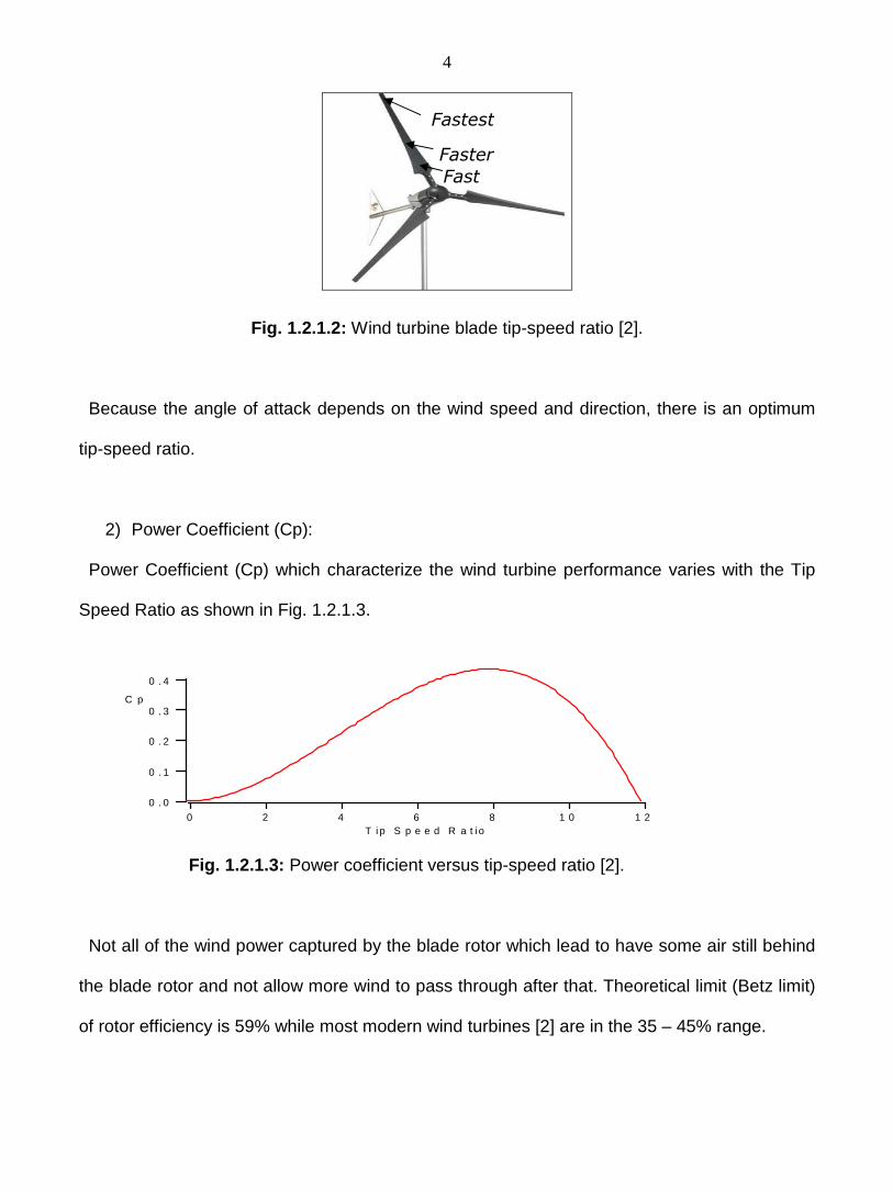
1) Pretwisting of the blade:

Pretwisting Blade should be twisted and tapered since speed through the air of a point on the

blade that changes along the distance from hub to tip. As shown in Fig. 1.2.1.2, the tip speed

ratio varies along the blade length to optimize the angle of attack along blade length, where the

blade should be twisted from root to tip. Tip-speed ratio (TSR) is the ratio of the speed of the

rotating blade tip to the speed of the free stream wind. There is an optimum angle of attack

which creates the highest lift to drag ratio.

TSR = Ω / where,

Ω : rotational speed in radians /sec

: Rotor Radius

: Wind “Free Stream” Velocity

4

Fig. 1.2.1.2: Wind turbine blade tip-speed ratio [2].

Because the angle of attack depends on the wind speed and direction, there is an optimum

tip-speed ratio.

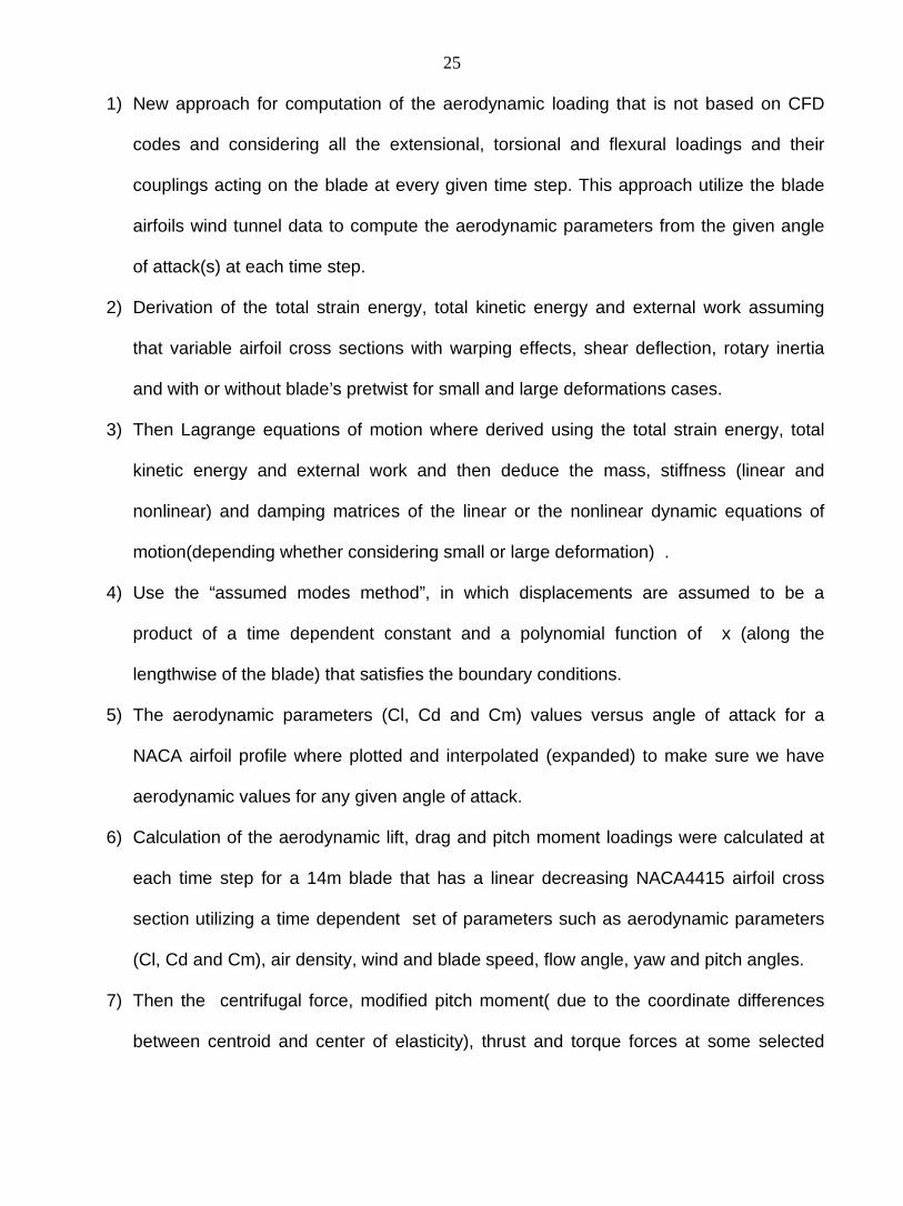
2) Power Coefficient (Cp):

Power Coefficient (Cp) which characterize the wind turbine performance varies with the Tip

Speed Ratio as shown in Fig. 1.2.1.3.

Fig. 1.2.1.3: Power coefficient versus tip-speed ratio [2].

Not all of the wind power captured by the blade rotor which lead to have some air still behind

the blade rotor and not allow more wind to pass through after that. Theoretical limit (Betz limit)

of rotor efficiency is 59% while most modern wind turbines [2] are in the 35 – 45% range.

Fast Faster Fastest

0 . 4

0 . 3

0 . 2

0 . 1

0 . 0

C p

1 2 1 0 8 6 4 2 0 T i p S p e e d R a t i o

5

Fig. 1.2.1.4: The wind turbine efficiency [2].

Wind turbine blades should be placed on high towers of steel and / or concrete due to the fact

that wind velocity and constancy increase with more height above ground. Rotors are on the

upwind side of the tower, in the less turbulent air.

Fig. 1.2.1.5: The Betz criterion [2].

3) Minimizing the blade weight:

Power extractable from the wind is proportional to the swept area A of the rotor:

P = A

6

where,

: is the Wind speed

: is the Air density

A: is equal to

This brings challenges that power increases with the square of blade length. The blade mass

and hence bending loads are more closely related to the cube of the blade length. Since mass

rises with rotor size faster than wind energy extracted, minimizing weight becomes increasingly

important as turbine size increases. This implies that we can win this challenge only if we build

the rotor blades with lighter composites materials including carbon fiber composite to beat the

squared-cubed law. Decreasing the blade mass is also important in wind turbine design due to

decreasing the load on the hub and shaft, and because the bending loads reverse at every

rotational cycle, the blade structure being alternately in compression (blade vertically above

the hub) and in tension (blade below). So decreasing the blade weight will decrease these

forces and the fatigue-inducing effect of the continual cycling. Another load cycle is

experienced due to wind gradient and the passage of blades from the bottom of the disc

sweep to an area of higher wind speed at the top. Horizontal axis wind turbines would avoid

this wind speed difference, but are less efficient.

4) Utilizing stiff materials:

Long blades can have large deformations with a big chance to strike the wind turbine tower

as they bend backwards in response to the wind aerodynamic loadings. In addition to the

aerodynamic loadings effect, the blades have an additional structural fatigue loading

created by the back pressure that generated by the eddies turbulence as the blades pass

7

by the wind support tower. Carefully engineered composites of great performance are

needed to provide fatigue resistance over design lives of 20 years or more.

Therefore, stiffness is another issue that blade manufacturers need to be met. This can be

countered by incorporating both high form stiffness and stiff materials, or in some cases by

‘prebending’ the blades in the toward-wind direction during manufacturing.

5) Blades with controlled twisting capabilities:

Blades can also fail due to excessive loadings during severe gust winds. To avoid failing,

blades are either automatically turn edgewise into wind to offer less resistance (pitch control),

or are shaped so that air stops flowing smoothly across the blade surface and, on reaching a

certain speed, breaks away destroying blade lift and dissipating energy (stall control).

An emerging possibility is to utilize the tailorability of composite properties to achieve bend-

twist coupling, such that when a blade bends away from the direction of an applied load it also

tends to twist. Given sufficient twist, this could provide an effective passive means of spilling

wind. In other scenarios, some adaptive blades are made to twist when actively signalled to

do so. Such mechanisms enable wind turbines to survive up to a wind gust of up to 100 mph

by preventing rotors from over speeding by rotating the blade tip to act as an aerodynamic

rotor brake.

6) Blade bending mode:

Another critical design issue is the frequency of blade excitation at which the blade can

damage and our need to avoid coincidence between this and blade rotational frequency. Any

such frequency convergence could lead to a damaging resonance condition under which

bending energy is amplified. Blades are usually configured to achieve a first blade bending

mode at least 1.5 times the rotational frequency of the rotor. As stiffening the blade increases

8

its natural (bending) frequency, over-stiffening must be avoided. Damping systems are

sometimes included to reduce the effects of any incipient modal vibration.

Endurance quality of materials are also important because blades must be out in the weather,

subject to wind, rain, salt, sand and dust erosion plus ultraviolet (UV). They may have to

endure thermal and humidity extremes and cycling. As they are high and exposed, blades

could attract lightning strikes, so effective protection is needed.

7) Acoustic issue:

Another factor, at least in well-populated developed countries, is acoustic footprint. Most of

the sound is emitted by the generators, by blade tips (which on the larger blades can

experience high airflow rates), and by insufficiently tapered blade trailing edges. Reinforced

plastics can be used for sound-absorbent housings and nacelle covers, and they are readily

molded into specific low-noise tip shapes. Environmental objectors also focus on the claimed

effects of wind turbines on birds, while blades can adversely affect air traffic control radars. (In

the UK, the Ministry of Defense reportedly rejects third party wind farm developments because

of the radar interference.

1.2.2 Structural Design

Considering the layout of wind turbine blades [3] as shown in Fig. 1.2.2.1, Fig. 1.2.2.2 and Fig.

1.2.2.3, the following design aspects are typically adopted:

Wing shells: The composite sandwich laminates are used towards leading and trailing

edges to increase the buckling resistance (edgewise loading). For the traditional blade

design, see Fig. 1.2.2.2 and Fig. 1.2.2.3 (top), the sandwich shell parts are transferred

9

into relatively thin monolithic composite laminates in the areas where the shells are

adhesively bonded to the main spar.

Main spar: The main spar usually extends from the root of the blade to a position close

to the tip. As mentioned, the primary function of the main spar is to transfer the

bladewise bending load, and thus it has to perform as a beam.

Spar cap: The primary function of the spar cap section is to carry the flapwise bending

moment, and it is usually made as a thick monolithic composite laminate, which for

some large blades could be a hybrid glass/carbon composite.

Spar flange: The primary function of these flanges are to carry the flapwise bending

moment, and they are usually made as thick monolithic composite laminates, which for

some large blades is made using hybrid glass/carbon composites. The main spar lay-up

usually include UD-layers to provide for the bending stiffness as well as off-axis or

angle-ply layers (often biaxial) to provide for the buckling resistance of the flange loaded

in compression (suction side of airfoil).

Internal webs/stiffeners: They carry the flapwise shear forces, and they are usually

made as composite sandwich plates with polymeric or balsa core and relatively with

biax laminate thin composite face sheets.

Fig. 1.2.2.1: The wind turbine blade components [3].

10

The sandwich design is chosen in order to enhance the resistance against in-plane shear

buckling. The rotational stiffness of the corners between the flanges and the webs for the

‘main spar design’ is of significant importance to accommodate for sufficient buckling

resistance of the flanges as well as to suppress the tendency of ovalization, the so-called

Brazier effect, of the blade and main spar cross sections during flapwise bending.

Fig. 1.2.2.2: (a) The wind turbine blade airfoil section [3]. (b) Design details of typical blade [3].

The same goes for the rotational stiffness of the joints between the spar cap and the internal

webs/stiffeners for the ‘spar cap/internal stiffener design’, however, to a somewhat lesser

degree. Various manufacturers use different design and manufacturing concepts. Alternative

designs, as compared with Fig. 1.2.2.1 and Fig. 1.2.2.2, may involve that the two wing shells

are joined with two or more internal webs (stiffeners) as shown schematically in Fig. 1.2.2.3.

In this conceptual design, the wing shells are manufactured with relatively thick so-called spar-

caps, which are usually monolithic composite laminates. Other wind turbine manufacturers

have adopted a manufacturing technique, where the entire blade structure including internal

webs/stiffeners is manufactured in one single process.

11

Irrespective of each of the below design concepts shown in Fig. 1.2.2.3 are used, the main

structural principles described earlier apply, i.e. the flapwise bending load is carried by a main

spar or a ‘main spar-like’ structure (constituted by the spar caps and internal webs/stiffeners),

and the edgewise load is carried by the shells.

Fig. 1.2.2.3: The different blade design concepts [3]

1.2.3 Barriers in Scaling up Conventional Blade Designs

Many fundamental barriers have been analyzed for the cost-effective scaling of the current

commercial blade designs and manufacturing methods over the size range of 100 m to120 m

diameter. The most substantial constraint is transportation costs, and these rise sharply for

lengths above 50 m (156 ft) and become prohibitive for long blades such as 60 m (187 ft). It is

expected that environmental considerations will prohibit the continued use of processes with

high emissions of volatile gasses, such as the open-mold wet lay-up that has been the wind

industry norm.

12

Another manufacturing issue for large blade is the bonding compounds. As blade size

becomes larger, it is natural for the gaps between bonded parts to grow also. However, the

bonding materials used for smaller blades do not scale well to increasing gap sizes, and blade

tooling and production costs for large blades increase rapidly as dimensional tolerances are

decreased. Gravity loading is not a barrier to scaling-up of the current conventional materials

and therefore blade designs over the size range are considered. However, materials and

designs that reduce blade weight will be of benefit for large scale megawatt blades, as this

facilitate the cost-effective of the scaling and reduce the need for reinforcements in the regions

of the trailing edge and at the blade root where transitions occur.

Another issue for turbine design is the use of larger rotors at a given turbine system rating. A

trend toward decreasing the power output per the unit rotor swept area (specific rating). It is

expected that turbine designs with low specific rating will be of continued interest for

deployment in the low wind speed sites of the Midwest United States. As specific rating is

decreased (i.e. blade lengths increase at a given rating), blade stiffness and the associated tip

deflections become increasingly critical for cost-effective blade design.

1.2.4 Blade Lift, Drag, Pitch Moment and Stall Phenomena

Lift, Drag and Pitch Moment

The two primary aerodynamic forces that act on wind turbine blade airfoil as shown in Fig.

1.2.4.1 are:

The lift, which acts perpendicular to the direction of wind flow.

The drag, which acts parallel to the direction of wind flow.

The pitch moment around the blade length axis.

13

Fig. 1.2.4.1: The lift and drag forces [4].

Wind turbine blade are shaped a lot like an airplane wing. They use an airfoil design where

one surface of the blade is somewhat rounded, while the other is relatively kind of flat. In one

simplified explanation of lift, when wind travels over the rounded, downwind face of the blade,

it has to move faster to reach the end of the blade in time to meet the wind traveling over the

flat, upwind face of the blade (facing the direction from which the wind is blowing). Since faster

moving air tends to rise in the atmosphere, the downwind, curved surface ends up with a low-

pressure pocket just above it. The low-pressure area sucks the blade in the downwind

direction, an effect known as "lift." On the upwind side of the blade, the wind is moving slower

and creating an area of higher pressure that pushes on the blade, trying to slow it down. Like

in the design of an airplane wing, a high lift-to-drag ratio is essential in designing an efficient

turbine blade. Turbine blades are twisted so they can always present an angle that takes

advantage of the ideal lift-to-drag force ratio.

Stall Phenomena

This phenomenon of stall is what happened when the wind’s speed angle of attack is climbed

to reach a value where all the sudden the air flow on the upper surface stops sticking to the

14

surface of the airfoil as shown in Fig. 1.2.4.2. Instead the air whirls around in an irregular

vortex (a condition which is also known as turbulence). All of a sudden the lift from the low

pressure on the upper surface of the airfoil disappears.

Fig. 1.2.4.2: The Flow around an Airfoil

Therefore, it is not easy to have an accurate selection of the required wind turbine blade

airfoils based on the wind tunnel testing data because:

1) Most wind tunnel data sets do not contain airfoil performance in stall, which is

commonly experienced by turbines operating in the field.

2) These wind tunnels have different operating conditions.

Also wind turbines are often roughened by soiling, for which there is very little data. Some

recent tests have shown that dynamic stall is a common occurrence for most wind turbines

operating in yawed, stalled, or turbulent conditions. Little dynamic stall data exists for the

airfoils of interest to a wind turbine designer. In summary, very little airfoil performance data

exits that is appropriate for wind turbine design.

These data should include airfoil performance at high angles of attack, rough leading edges

(bug simulation), and steady and unsteady angles of attack. The unsteady angles of attack

are a result of the blade deflections due the changes in the applied aerodynamical load. To

illustrate more, let us look at below Fig.1.2.4.3 where we have taken one rotor blade off its hub,

and then looking from the hub towards the tip, at the back side (the lee side) of the rotor blade.

15

Fig. 1.2.4.3: The variation of the Angle of attack at hub and tip.

For example, consider a typical wind blowing say at 8 m/s and 16 m/s from the bottom of Fig.

1.2.4.3, the tip of the blade rotates towards the left side of the Fig. 1.2.4.3. In this Figure, we

can see how the angle of attack of the wind changes much more dramatically at the root of the

blade (yellow line) than at the tip of the blade (red line), as the wind changes. If the wind

becomes powerful enough to make the blade stall, it will start stalling at the root of the blade.

1.2.5 Wind Turbine Blade Materials Historically, wind turbine blades have been constructed using different materials including

wood, fiberglass . But recently, most of these blades are made of fiberglass with the use of

carbon fiber for some critical areas that need local reinforcement. Also the use of carbon fiber

in the load-bearing spar structure of the blade has been identified as a substantial promise for

cost effective weight reductions beside the increased stiffness. Analyses performed earlier by

some researchers predicted mass reductions of approximately up to 30% and a cost decrease

up to 15% when use the carbon fiber compared the baseline fiberglass blade. This study

16

assumed that the fiberglass / carbon hybrid material extended the entire length of the blade

spar. Stitched hybrid fabrics and other automated technologies also have potential benefit in

this area.

1.2.5.1 Different Blades Composites Manufacturing Processes

Maintaining fiber straightness (see Fig. 1.2.5.1.1 ) is critical to achieve desirable compressive

strength properties from composite materials [1]. While carbon fibers tend to have excellent

stiffness and tensile strength properties, realizing the full benefits from carbon fibers will

require fabric/preform architectures that also result in good compressive strength. MSU has

been testing coupons of large-tow carbon to determine compressive static strength, fatigue

strength, and effect of fiber waviness on material performance.

Fig. 1.2.5.1.1: Composite materials [1].

17

The primary bending loads shown in Fig. 1.2.5.1.2 are from aerodynamic forces, and are

carried by a structural spar. In North America wind turbine design community, the spar flanges

are termed “spa caps”, while European designers tend to use the term “griders”. For

megawatt-scale blades, two shear webs are common, forming a box beam as shown in

Figure1. Smaller blades, and some MW-scale designs, use a single shear web, or I-beam

configuration. The structural spar is enclosed in two shells (skins) which form the aerodynamic

profile. The skins and shear webs are typically sandwich-style laminate. The composites

laminated parts are either glass or carbon fiber-reinforced polymers, while the sandwich core

materials may be polymeric foams (PVC or BMI), balsa wood core or less frequently of

honeycomb type.

Fig. 1.2.5.1.2: The typical wind turbine blade structural layout [5].

For blade sizes up to 30 m, the most common manufacturing approach has been open mold,

wet lay-up. The most notable exception to that approach is Vestas Wind Systems, which has

experience in using the prepreg fiberglass for their blade manufacturing. Despite that several

manufacturers are using open-mold, wet lay-up processes, become more and more stringent

environmental restrictions to move manufacturers toward processes that have lower emissions.

18

Currently, the most common replacement for traditional methods use one of the following two

methods: A) Preimpregnated materials and B) Resin infusion, with VARTM (most common

infusion method). Both prepreg and VARTM materials have particular design challenges for

manufacturing the relatively thick laminate that typical for large wind turbine blades. For

VARTM processes, the permeability of the dry preform determines the rate of resin penetration

through the material thickness. For prepreg material, sufficient bleeding is required to avoid

resin-rich areas and eliminate voids from trapped gasses.

Another alternative is the partially preimpregnated fabric, marketed by SP Systems and

Hexcel Composites under the name of SPRINT and HexFIT respectively. When laid-up, the

dry fabric regions provide paths for air to flow, and vacuum can be used to evacuate the part

prior to heating. Under heat and pressure, the resin flows into the dry fabric regions to

complete the impregnation. High temperature post-cure is desirable for both prepreg and

VARTM processes. Current prepreg materials require higher cure temperatures (90°C– 110°C)

than epoxies used in VARTM processes (60°C–65°C). Heati ng and temperature control /

monitoring becomes increasingly difficult as the laminate thickness is increased.

Mold and tooling costs are also strongly affected by the heat requirements of the cure cycle.

In all cases, achieving the desired laminate quality requires a trade-off between the extent of

fiber compaction, fabric/ preform architecture, resin viscosity, and the time/temperature profile

of the infusion and cure cycles.

The use of automated preforming and lay-up technologies are potential alternatives to hand

lay-up in the blade molds. Advantages could include improved quality control in fiber/fabric

placement and a decrease in both hand labor and production cycle times. The overwhelming

majority of turbine original equipment manufacturers (OEMs) and third-party blade

manufacturers use a VARTM process. It is notable that the OEMs with the #1 (Vestas) and #3

(Gamesa) shares of the 2007 global market primarily use prepreg material which is the

19

standard process for carbon current commercial blades. The differences between the

composite prepreg technology and the vacuum assisted vacuum infusion (VARTM or

variations of this process) are shown below in Table 1.2.5.1.1.

Prepreg Materials Infusion RTM Advantages Advantages Advantages

Homogeneous distribution of resin content & higher fiber

volume than any other process. Lower raw material prices. Higher production rates.

Quality & controlled process. Curing cycles at 60-70 C.

It is becoming an alternative for semi-

structural parts.

Improving process control every year

Disadvantages Disadvantages Disadvantages

Raw material prices increase more than 30%

Difficulties to guarantee Resin flow through thick laminates and wet-out of

carbon fibers.

Resin content higher- lower mechanical

properties. Logistic and storage under

restrictive T/RH conditions controlled

Long curing cycles at 120 C. Quality- skilled labor

required.

Blade surface areas are too large for one shot

processes.

Table 1.2.5.1.1: The comparison between Prepreg, Infusion and RTM [1].

1.2.5.2 The Fiber Alignment in Fiber Carbon The small Business Innovation Research (SBIR) is currently looking on alternatives to

prepreg materials, by evaluating different materials with a unidirectional carbon fabric that

would achieve good structural properties in a VARTM infusion process. In one scenario, the

fabric may infuse well, but waviness in the fibers is a restriction for the carbon to achieve its

20

potential strength, particularly in compression. In the other scenario, the fabric architecture

may have very good fiber alignment, but not allow resin penetration through the thickness.

For most fabric architectures, it is generally true that any feature that promotes through-the –

thickness infusion will result in fiber misalignment and corresponding reductions in

compressive strength. Fig. 1.2.5.2.1 shows a typical stitched unidirectional fabric using large-

tow carbon fibers.

Fig. 1.2.5.2.1: Stitched unidirectional carbon fabric with induced waviness [5].

1.2.6 Varying Properties along the Blade

Wind turbine blades are built from orthotropic materials ( where the material parameters are

direction dependent) that are made of two or more distinct materials put together such as

sandwich plates. Fiber composites are built of several layers, where each layer is composed

of fiber reinforcements embedded in a continuous phase termed the matrix. In general, all

layers can be made of different materials. Moreover, the direction of the fibers in each layer,

according to common axes, influences on the properties of the whole composite. This makes

the expressions for the effective material properties for the fiber composite more complicated,

and more than two material coefficients are required.

Material Stiffness Matrix for a Single Layer

In the same way as for the isotropic thin plate, lets us assume plane stress conditions to

prevail. Thus, for a single layer of unidirectional, continuous fibers, referred to local axes for

the layer, it can be shown that the material stiffness matrix may be ex

where k is the layer number, and

The fiber direction is called the longitudinal direction (L), and the direction normal to the fibers

is the transverse direction (T), see

where,

EL and ET : are the elastic moduli in the longitudinal and the transverse directions, respecti

υLT : is the major Poisson ratio (give

υTL : is the minor Poisson’s ratio (give

GLT : is the shear modulus.

These four material constants are related through this re

21

Material Stiffness Matrix for a Single Layer

same way as for the isotropic thin plate, lets us assume plane stress conditions to


the layer, it can be shown that the material stiffness matrix may be expressed as:

where k is the layer number, and


is the transverse direction (T), see Fig. 1.2.6.1.

are the elastic moduli in the longitudinal and the transverse directions, respecti

: is the major Poisson ratio (give transverse strain caused by longitudinal stress

: is the minor Poisson’s ratio (give the longitudinal strain resulting from a transverse stress)

nts are related through this relation:

same way as for the isotropic thin plate, lets us assume plane stress conditions to


pressed as:

(1.2.6.1)

(1.2.6.2)


are the elastic moduli in the longitudinal and the transverse directions, respectively

transverse strain caused by longitudinal stress)

ulting from a transverse stress)

Fig. 1.2.6.1: The fiber direction in a composite build of unidirectional, continuous fibers

Therefore, four independent material parameters (for each layer) are required for such

orthotropic problems in 2D. Using transformation matrices, it can be shown that the matrix for

a single layer, referred to global

where,

In these expressions ө is the angle between the positive global xbar axis and positive local x

axis for the layer and k is the layer number.

the composite can then be expressed as:

22

The fiber direction in a composite build of unidirectional, continuous fibers



a single layer, referred to global ( ) axes, is:

is the angle between the positive global xbar axis and positive local x

yer and k is the layer number. The stress-strain relation for one single layer of

the composite can then be expressed as:

The fiber direction in a composite build of unidirectional, continuous fibers [6].



(1.2.6.3)

(1.2.6.4)

is the angle between the positive global xbar axis and positive local x

strain relation for one single layer of

To get the material properties for the whole laminate, we sum up for all the layers i.e. integrate

over the plate thickness:

where ( hk - hk-1 ) is the thickness of layer number k.

whole matrix is:

1.3 Research Motivation and Objectives

1.3.1 Research Motivation Over the last two decades, continually growing energy demands as well as global warming

and other pollution concerns have drawn considerable attention t

renewable sources of energy including the wind energy. The

development of wind turbine, in recent years, has been focused on the following research

areas:

Developing the blade composite materials to

blades.

23


e thickness of layer number k. By the way, the stiffness matrix for the

1.3 Research Motivation and Objectives

Motivation

Over the last two decades, continually growing energy demands as well as global warming

and other pollution concerns have drawn considerable attention to the need for alternative

renewable sources of energy including the wind energy. The cutting edge


Developing the blade composite materials to have more stiff but less weight

(1.2.6.5)


(1.2.6.6)

stiffness matrix for the

(1.2.6.7)

Over the last two decades, continually growing energy demands as well as global warming

o the need for alternative and

cutting edge technological


have more stiff but less weight

24

Developing new advanced methods to optimize the blade aerodynamic structure.

Computing the aerodynamic loadings that act on the blade structure using CFD

codes.

Also a number of approximate theories used for the pre-twisted beam (that is similar to

helicopter rotor blades) have been developed by different researchers to analyze its

complex geometry. A carefully selected sample of the relevant literature on the wind

turbine blade ( as explained in Chapter 4 Introduction), show that there is a need to expand

the wind blade research to include more of these research factors that were taken

separately in a one complete research, such factors will include:

Computing the load vector at each time step and the mass, stiffness matrices of

the dynamic equation of motion utilizing an analytical solution and considering all

the extensional, torsional and flexural loadings acting on the blade with their

couplings.

Variable airfoil cross-sections.

Warping effects.

Shear deflection, rotary inertia and with or without blade’s pretwist.

Formulations should include both the linear small deformation case and the

nonlinear large deformation case.

To the best knowledge of the author the simultaneous inclusion of all these factors has not

been done before.

1.3.2 Research Objectives The objective of the present work is to conduct the following research on the wind turbine

blade, using an analytical energy approach:

25

1) New approach for computation of the aerodynamic loading that is not based on CFD

codes and considering all the extensional, torsional and flexural loadings and their

couplings acting on the blade at every given time step. This approach utilize the blade

airfoils wind tunnel data to compute the aerodynamic parameters from the given angle

of attack(s) at each time step.

2) Derivation of the total strain energy, total kinetic energy and external work assuming

that variable airfoil cross sections with warping effects, shear deflection, rotary inertia

and with or without blade’s pretwist for small and large deformations cases.

3) Then Lagrange equations of motion where derived using the total strain energy, total

kinetic energy and external work and then deduce the mass, stiffness (linear and

nonlinear) and damping matrices of the linear or the nonlinear dynamic equations of

motion(depending whether considering small or large deformation) .

4) Use the “assumed modes method”, in which displacements are assumed to be a

product of a time dependent constant and a polynomial function of x (along the

lengthwise of the blade) that satisfies the boundary conditions.

5) The aerodynamic parameters (Cl, Cd and Cm) values versus angle of attack for a

NACA airfoil profile where plotted and interpolated (expanded) to make sure we have

aerodynamic values for any given angle of attack.

6) Calculation of the aerodynamic lift, drag and pitch moment loadings were calculated at

each time step for a 14m blade that has a linear decreasing NACA4415 airfoil cross

section utilizing a time dependent set of parameters such as aerodynamic parameters

(Cl, Cd and Cm), air density, wind and blade speed, flow angle, yaw and pitch angles.

7) Then the centrifugal force, modified pitch moment( due to the coordinate differences

between centroid and center of elasticity), thrust and torque forces at some selected

26

airfoil stations were calculated using the Airfoil wind tunnel aerodynamical parameters

data ( Cl, Cd and Cm).

8) Create a MATLAB code to contain all the above Mathematical Formulations including

the interpolation of all the stations’ forces and moments to obtain them as a function of x,

using a built-in interpolation algorithm within this code .

9) Using the MATLAB code, compute the six degree of freedom at any point on the blade,

for both linear and nonlinear cases (small and large deformations respectively).

10) For the linear small deformation case, compare the MATLAB code displacement result

plots with Younsi et al. for the same blade example.

11) Create an ls-dyna code that has the same blade inputs of geometrical and material

properties and aerodynamic loadings.

12) For the linear small deformation case, compare its displacement result plots with

those of the MATLAB code ( since the nonlinear case is not found in the literature to

compare).

13) Establish the mathematical relationship for the coupling between the blade twist around

the blade and the angle of attack at every time step to update the angle of attack on the

next time step by adding or subtracting the twist angle from the angle of attack.

1.4 Aerodynamics Loads

1.4.1 Airfoil’s Load Layout

The analysis of the state of load on the wind turbine blade is intended to verify whether the

turbine will withstand the action of load within appropriate safety range. Various cases of load

27

on the blade, resulting from the action of various external factors on the turbine, have to be

considered. The following types of states of loadings on a wind turbine blade can be

distinguished:

The aerodynamic loads of a wind turbine blade are shown in Fig.1.4.1.1.

The mass loads, as the wind turbine blade is slender, the loads associated with its

inertia are limited to the loads generated by its weight, which causes sinusoidal loads

the frequency of which corresponds to the rotor. Both mass and aerodynamic loads

were investigated.

Fig. 1.4.1.1: The local forces on the blade [7]

1.4.2 Simple Load Formulas / Model The loading on a wind turbine blade as shown in the below Fig.1.4.2.1 consist of the following:

The flapwise and edgewise bending due to the loadings on the blade (skew bending).

28

The gravitational loads, which change direction during the rotation of the blade, and

which mainly generate edgewise bending loading.

The torsional loading because the shear resultants of the flap- and edgewise loads do

not go through the shear centre of the blade section.

The normal loading due to the rotation of the blade (inertia forces).

The relative small loads due to pitch de-accelerations and accelerations.

The latter three have very little influence on the design loads, and it is the flapwise and

edgewise loads that determine the structural design and the blade cross sections. The spar

carries most of the flapwise bending, while the edgewise bending primarily is carried of by the

leading and trailing edges of the aerodynamic profile, which are strengthened due to this.

Below Figure1.4.2.1 illustrates the components of airspeed and force acting on an airfoil

section on a wind turbine blade. at a radial distance r from the axis of rotation. The view in

these schematic diagrams is from the blade hub toward the tip. According to the BEM theory,

airloads on a section of an airfoil are proportional to the dynamic pressure at only that section.

Lift and Drag Forces

CL and CD coefficients are proportionality constants that is required for the calculation of the L

and D forces as shown in Fig. 1.4.2.1:

L = CL pd C (1.4.2.1)

D = CD pd C (1.4.2.2)

pd = 0.5 ρ Vrel 2 (1.4.2.3)

29

Fig. 1.4.2.1: The wind and force vectors acting on an airfoil [7].

which implies that:

Lift Force: L = 0.5 ρ Vrel 2 C CL (1.4.2.6)

Drag Force: D = 0.5 ρ Vrel 2 C CD (1.4.2.7)

Thrust Force: FN = L cos φ + D sin φ (1.4.2.8)

Torque Force: FT = L sin φ − D cos φ (1.4.2.9)

where,

L: is the lift force per unit span; intensity of force perpendicular to relative airspeed (lb/ft)

D: is the drag force per unit span; intensity of force parallel to relative airspeed (lb/ft)

CL, CD: are the lift and drag coefficients of the section respectively

C: is the chord length of aerodynamic profile (ft)

pd: is the aerodynamic pressure (lb/ft2)

ρ: is the air density (slugs/ft2)

φ: is the wind flow angle

30

1.5 Blade Element Momentum Theory

Blade Element Momentum Theory relates two methods to examine how a wind turbine

operates. The first method is to use a momentum balance on a rotating annular stream tube

passing through a turbine and the second method is to examine the forces generated by the

aerofoil lift and drag coefficients at various sections along the blade as explained in [8].

Momentum Theory

Consider the stream tube around a wind turbine shown in Fig. 1.5.1 and explained in

reference [8]. Four stations are shown in the diagram 1, some way upstream of the turbine, 2

just before the blades, 3 just after the blades and 4 some way downstream of the blades.

Between 2 and 3 energy is extracted from the wind and there is a change in pressure as a

result. Apply Bernoulli’s equation, assuming that p1 = p4 and that V2 = V3 .

Fig. 1.5.1: Axial stream tube around a wind turbine [8].

We can also assume that between 1 and 2 and between 3 and 4 the flow is frictionless:

(1.5.1)

31

Noting that force is pressure multiplied by area:

(1.5.2) or,

(1.5.3) Define a as the axial induction factor:

(1.5.4) It can also be shown that:

(1.5.5)

(1.5.6) Substitute, implies:

(1.5.7)

Rotating Annular Stream tube

Applying the conservation of angular momentum in the annular stream tube shown in

Fig.1.5.2, where between 2 and 3 the rotation of the turbine imparts a rotation onto the blade

wake. Considering that the blade wake rotates with an angular velocity ω and the blades

rotate with an angular velocity of Ω. From basic physics, as explained in reference [8], the

following equations can be obtained:

32

Fig. 1.5.2: Rotating annular stream tube [8].

(1.5.8)

(1.5.9)

(1.5.10)

(1.5.11)

So for a small element the corresponding torque will be:

(1.5.12) For the rotating annular element:

(1.5.13)

33

Fig. 1.5.3: Rotating annular stream tube notation [8].

(1.5.14)

(1.5.15) Define angular induction factor a׳ :

(1.5.16)

(1.5.17)

Momentum theory has therefore yielded equations for the axial (Eqn 1.5.17) and tangential

force (Eqn 1.6.1.17) on an annular element of fluid.

Blade Element Theory

Blade element theory relies on the following two key assumptions [8]:

1) There are no aerodynamic interactions between different blade elements.

2) The forces on the blade elements are solely determined by the lift and drag

coefficients.

34

Consider a blade divided up into N elements as shown in Fig. 1.5.4. Each of the blade

elements will experience a slightly different flow as they have a different rotational speed Ωr, a

different chord length c and a different twist angle β. Blade element theory involves dividing up

the blade into a sufficient number (usually between ten and twenty) of elements and

calculating the flow at each one. Overall performance characteristics are determined by

numerical integration along the blade span.

Fig. 1.5.4: The blade different stations [8] Relative Flow

Lift and drag coefficient data area available for a variety of aerofoils from wind tunnel data.

Since most wind tunnel testing is done with the aerofoil stationary we need to relate the flow

over the moving aerofoil to that of the stationary test. To do this we use the relative velocity

over the aerofoil. In practice the flow is turned slightly as it passes over the aerofoil so in order

to obtain a more accurate estimate of aerofoil performance an average of inlet and exit flow

conditions is used to estimate performance. The flow around the blades starts at station 2 in

Fig. 1.5.2. and Fig. 1.5.1. and ends at station 3. At inlet to the blade the flow is not rotating, at

35

exit from the blade row the flow rotates at rotational speed ω. That is over the blade row wake

rotation has been introduced.

The average rotational flow over the blade due to wake rotation is therefore ω/2. The blade is

rotating with speed Ω which lead that the average tangential velocity of the blade is Ωr + 0.5ωr

as shown in Fig. 1.5.5.

Fig. 1.5.5: Flow onto the turbine blade [8]. Examining Fig. 1.5.5, we can immediately note that:

(1.5.18) but since V2 = V1 V(1-a), implies:

(1.5.19) where V is used to represent the incoming flow velocity V1 .

36

The value of β will vary from blade element to blade element. But the local tip speed ratio λr

is defined as:

(1.5.20) This leads to a further simplification for tanβ :

(1.5.21) From Fig. 1.5.5 the following relation is obvious:

(1.5.22) Blade Elements

The forces on the blade element are shown in Fig. 1.5.6, note that by definition the lift and

drag forces are perpendicular and parallel to the incoming flow. For each blade element one

can conclude:

Fig. 1.5.6: The forces on the turbine blade [8].

37

(1.5.23)

(1.5.24) dL and dD can be found from the definition of the lift and drag coefficients as follows:

(1.5.25)

(1.5.26) where dL and dD are the lift and drag forces on the blade element respectively.

If there are B blades, by combining Equation (1.5.23) and Equation (1.5.25), it can be shown that:

(1.5.27)

(1.5.28) The Torque on an element, dT is simply the tangential force multiplied by the radius.

(1.5.29) The effect of the drag force is clearly seen in the equations, an increase in thrust force on the

machine and a decrease in torque (and power output). These equations can be made more

useful by noting that and W can be expressed in terms of induction factors etc. i.e. Equations

(1.5.21) and (1.5.22). Substituting and carrying out some algebra yields:

38

(1.5.30)

(1.5.31) where σ ׳ is the local solidity:

(1.5.32) Tip Loss Correction

Losses at the tip of the turbine blade are introduced in a similar manner to those found in

wind tip vorticies on turbine blades. It can be accounted for these losses in BEM theory by

means of a correction factor. This correction factor Q varies from 0 to 1 and simulates the

reduction in forces along the blade.

(1.5.33)

The results from cos-1 must be in radians. Apply the tip loss correction factor to Eqn 1.5.7 and

Eqn 1.5.17:

(1.5.34)

(1.5.35) From the above, we now have four equations, two dervied from momentum theory which

express the axial thrust and the torque in terms of flow parameters (Equations (1.5.35) and

(1.5.34):

(1.5.36)

39

(1.5.37)

Also we have two equations derived from considering the blade forces which express the

axial force and torque in terms of the lift and drag coefficients of the aerofoil Eqn 1.5.30 and

Eqn 1.5.31:

(1.5.38)

(1.5.39) To calculate rotor performance Eqn 1.5.34 and Eqn 1.5.35 from a momentum balance are

equated with Eqn 1.5.30 and Eqn 1.5.31:

(1.5.40)

(1.5.41) Power Output Eqn 1.5.40 and Eqn 1.5.41 are used in the blade design procedure. The contribution to the

total power from each annulus is [8]:

(1.5.42) The total power from the rotor is:

(1.5.43) where rh is the hub radius. The power coefficient Cp is given by:

40

(1.5.44) Using Eqn 1.5.31, it is possible to develop an integral for the power coefficient directly. After some algebra:

(1.5.45)

Blade Design Procedure The following is a blade design procedure as explained by reference [8]:

1) Determine the rotor diameter required from site conditions and P = 0.5Cp ρηπR2V 3

where,

P: is the power output

Cp : is the expected coefficient of performance (0.4 for a modern three bladed wind turbine)

η : is the expected electrical and mechanical efficiencies (0.9 is a suitable value)

R : is the tip radius

V : is the expected wind velocity

Table 1.5.1: The number of blades [8].

41

2) Choose a tip speed ratio for the machine. For water pumping pick 1 < λ < 3 (which

gives a high torque) and for electrical power generation pick 4 < λ < 10.

3) Choose a number of blades B, using Table 1.5.1, which is based on practical experience.

4) Select an airfoil. For λ < 3 curved plates can be used.

5) Obtain and examine lift and drag coefficient curves for the aerofoil in question.

6) Choose the design aerodynamic conditions for each aerofoil. Typically select 80% of the

maximum lift value.

7) Divide the blade into N elements. Typically 10 to 20 elements would be used.

8) As a first guess for the blade twist and chord, use the blade shape derived with wake

rotation, zero drag and zero tip losses. Note that these equations provide an initial guess only.

The equations are given as follows:

(1.5.46)

(1.5.47)

(1.5.48) 9) Calculate rotor performance and then modify the design as necessary. This is an

iterative process. The application of BEM can be sometimes confusing as it can be used to

either to design i.e. select γ and c or to analyze the performance of a blade.

It should be noted that different aerofoil profiles may be used at different spans of the blade,

for example, a thick aerofoil may be selected for the hub to give greater strength.

42

Chapter 2

Literature Review on Blade Different Formulations & Research Plan

2.1 Introduction

The wind turbine blade can be considered as a pretwisted beam. Hence it is essential to

understand how to analyze and work with beams. Beam element is a versatile line-element

where in general it has six degrees of freedom at each node, which include three translational

displacements along the x, y, and z directions and three rotational displacements about the x,

y, and z directions as shown on the right side node of the beam of Fig. 2.1.1 shows the

positive directions of these displacements.

Fig. 2.1.1: Beam element with six degrees of freedom at each node.

Beam element can be used to simulate a slender structure that has a uniform cross- section.

The stiffness constant of a beam element is derived by combining the stiffness constants of a

beam under pure bending, a truss element, and a torsion bar. A beam element can represent

a beam in bending, a truss element, and a bar in torsion. To derive the element stiffness

equation for a beam element that subjected to all these loadings, we start first by deriving the

43

stiffness equation of a beam subjected to bending loading only, and then superimpose the

stiffness of a truss subjected to axial loading only and then superimpose the stiffness of a bar

subjected to torsional loading only to obtain the resultant stiffness equation for all loadings .

2.2 Aeroelasticity

Aeroelasticity is the study of the mutual interaction between the aerodynamic and elastic

forces, and the influence of this interaction on blade design [9]. Wind turbine Blade is a very

flexible, and this flexibility is the main factor for the various types of the aeroelastic

phonemena.

The aeroelastic phonemena happen when the structural deformations induce some additional

aerodynamic forces which in turn produce some additional structural deformations that again

induce more aerodynamic forces. The dynamic aeroelasticity phenomena is the one involves

the interactions among all the inertial, aerodynamical, and elastic forces, while the static

aeroelastic phenomena is the one involves the interations between aerodynamical and elastic

forces. Fig. 2.2.1 show the relationship between the all these forces.

For wind turbine blade, such interactions are tremendous because of the couplings among all

the aerodynamics axial, bending and torsional loadings (forces and moments) acting on the

blade. These interactions may tend to become less and less until a condition of equilibrium

stability is reached, or they may tend to diverge and destroy the structure.

The static aeroelasticity includes the following:

1) Static divergence

2) Load redistribution

3) Control reversal and effectiveness

4) Aeroelastic effects on static stability

And the dynamic Aeroelasticity includes the following:

1) Flutter

2) Buffeting

3) Dynamic response

4) Aero-elastic effects on dynamic stability

Fig. 2.2.1:

The following are explanation of some common aero

Flutter : is a dynamic instability occurring in a blade at a speed called the flutter speed,

where the elasticity of the structure plays an essential part in the instability.

Buffeting : are the transient vibrations of blade structural components due to aero

dynamic impulses produced by the wake around the blade, or other components of the

wind turbine mild.

Dynamic response : is the transient response of blade structural compon

produced by quick applied loads due to gusts, gun reactions, abrupt control motions,

moving shock waves, or other dynamic loads.

Load Distribution : It is due to the influence of the elastic deformations of the blade

structure on the distribution of

44

And the dynamic Aeroelasticity includes the following:

elastic effects on dynamic stability

Fig. 2.2.1: The summary of loadings and their responses

The following are explanation of some common aero-elastic terms:

: is a dynamic instability occurring in a blade at a speed called the flutter speed,


: are the transient vibrations of blade structural components due to aero


: is the transient response of blade structural compon


moving shock waves, or other dynamic loads.

: It is due to the influence of the elastic deformations of the blade

structure on the distribution of aero-dynamic pressures over that structure.

responses.

: is a dynamic instability occurring in a blade at a speed called the flutter speed,


: are the transient vibrations of blade structural components due to aero-


: is the transient response of blade structural components


: It is due to the influence of the elastic deformations of the blade

dynamic pressures over that structure.

Divergence : is the static instability of the wind turbine blade, at a speed called the

divergence speed, where the elasticity of the blade surface plays an essential role in the

instability.

Control Effectiveness : It is due to the influence of elastic deformations of the blade

structure on the controllability of the blade.

2.3 Large Deformation versus Small Deformation When the deformation of the wind turbine blade is small i.e. less than 10% of

blade, we can use the deformation linear is linear and this happens when the change i

volume is almost negligible. However, once we have deformations that are greater than

of the length of the blade, we should use the appropriate st

for for this large deformation.

account for that large deformation of the blade.

The above strain tensor is known as the Green

order tensor because it has two independent indices. An obvious question is how the Green

Lagrange strain tensor compares to the small deformation strain tensor that we did make

assumptions to derive. We start by substituting the displace

gradient tensor to obtain:

We obtain the above because when a quantity is multiplied by the kronecker delta we obtain

the same quantity back, with the free index from the kroneck

repeated index on the quantity it is multiplying. It should be noted that the large deformation

45

: is the static instability of the wind turbine blade, at a speed called the


: It is due to the influence of elastic deformations of the blade

structure on the controllability of the blade.

Large Deformation versus Small Deformation

When the deformation of the wind turbine blade is small i.e. less than 10% of

blade, we can use the deformation linear is linear and this happens when the change i

However, once we have deformations that are greater than

we should use the appropriate stress and strain tensors to account

for for this large deformation. We should also use the appropriate constitutive relations that

account for that large deformation of the blade.

The above strain tensor is known as the Green-Lagrange strain tensor. It i

order tensor because it has two independent indices. An obvious question is how the Green


assumptions to derive. We start by substituting the displacement equation for the deformation


the same quantity back, with the free index from the kronecker delta being exchanged with the


: is the static instability of the wind turbine blade, at a speed called the


: It is due to the influence of elastic deformations of the blade

When the deformation of the wind turbine blade is small i.e. less than 10% of the length of the

blade, we can use the deformation linear is linear and this happens when the change in

However, once we have deformations that are greater than 10%

ress and strain tensors to account

We should also use the appropriate constitutive relations that

Lagrange strain tensor. It is also a second

order tensor because it has two independent indices. An obvious question is how the Green-


ment equation for the deformation

(2.3.1)


er delta being exchanged with the


46

strain tensor includes many nonlinear higher order terms which indicate that all the large

deformation analyses are nonlinear. Recall that the small deformation strain tensor is:

(2.3.2)

Therefore by assuming that the deformation is small, we drop all the nonlinear higher order

terms from the Green-Lagrange strain tensor and keep the linear terms only.

2.4 Aeroelastic Coupling Schemes Due to changes of aerodynamics loads on the wind turbine blades, these blades twist. Due

that twisting, there is a direct influence on the angle of attack, changing loads and affecting

output power. This is directly exploited in classic pitch control used in not only wind turbines

but in rotors of all types. When the pitch changes are rapid enough, they can affect not only

average loads and power, but vibratory loads as well, influencing fatigue life throughout the

system. Even quite small angles of twist can have significant impact.

Any time the wind turbine blade becomes aeroelastically “active” (i.e. when the elastic

deformations play a role in the aerodynamic loading), the dynamic stability of the blade will be

affected. Veers et al. [10] address two of the most common stability constraints, namely flutter

and divergence.

Flutter is the condition where the phasing between the aerodynamic load fluctuations and

elastic deformations are such that a resonant condition is achieved. Every wing will have a

flutter boundary at some speed. For wind turbines the boundary is defined at the rotational

47

speed (typically determined in still air) at which the blade will flutter. The stability margin is the

difference between the flutter speed and normal operating speed.

Divergence is a quasi-static condition where the blade twists in response to increasing load in

a direction that further increases the load. If this condition exists on a blade there will be an

operating speed at which the increase in loads caused by the deformation exceeds the ability

of the blade to resist the load, called divergence.

The stability boundaries were determined with respect to the amount of twist coupling built

into the blade. A coupling coefficient, α, was defined to facilitate the generic examination of

stability effects.

For a blade with bending-twist coupling, the matrix equation for blade bending and twisting

strains εb and εt due to bending and twisting loads Mb and Mt are:

(2.4.1)

where EI and GK are the beam bending and torsional stiffness, respectively. The coupling

coefficient, g , is constrained to values that keep the system positive definite. The range of

realizable g values is limited to:

(2.4.2)

It should noted that equation (1.6.2.1) that include the coupling between bending and twisting

loads will change later when I include the couplings of all other possible aerodynamic loading

acting on the blade in addition to the inclusion of the nonlinear higher order terms due the large

nonlinear large deformation assumption.

48

2.5 Optimization of Blade Design

The aerodynamic and structural design of rotors for horizontal axis wind turbine (HAWT)

involves many conflicting requirements, for example, maximum performance, minimum loads

and minimum noise. The wind turbine operates in very different conditions from normal

variation in wind speed to extreme wind occurrences. Optimum efficiency is not obtainable in

the entire wind speed range, since power regulation is needed to prevent generator burnout at

high wind speeds. Optimum efficiency is limited to a single-design wind speed for stall

regulated HAWT with fixed speed of rotation.

Several optimization methods exist . They are typically based on a numerical optimization

algorithm. Multipoint design methods have a larger degree of flexibility for optimization

objective and the majority allows multiple constraints. The first generation of the methods

involved maximum annual energy production as objective, since this includes off-design

performance with no or only few constraints on loads. The reported improvements of the

annual energy production are promising, but they often arrive from an increase in swept area

for the same generator size.

Unfortunately, this will result in larger loads on tower and the blade roots. Actually, the

increase in loads often exceeds the increase in energy yield. Optimum design should not be

restricted to aerodynamic performance. In most of the cases, the key factor is the minimum

cost of energy, and this should be the objective. This leads to the development of second

generation design tools, where the optimization objective is the minimization of the cost of

energy. Cost of energy is by definition the ratio of the total costs from manufacture and

erection of the wind turbine to the annual energy production. Proper cost estimate involves

calculation of fatigue loads as well as extreme loads on all main components and a cost

function describing the coupling between design loads and cost. Using a multi-disciplinary

design method for direct shape design of HAWT rotors.

49

In the present research, the author main concern is to use a numerical optimization, where

the objective is to have the displacements and rotations ( six degrees of freedom) at the tip of

the blade under a certain maximum limit with a set of multiple constraints that are allowed i.e.

extreme loads, material Young’s modulus and/or material density.

The optimization of the wind turbine blade displacements and rotations is a feature that can be

done in the MATLAB code and is not really the concentration of this research. The design of

any blade rotor can be utilized to demonstrate the capabilities of this design method within the

MATLAB code. It should be noted that:

Loads constraints and cost estimation were important for the applicability of the

optimization results.

With traditional airfoil characteristics and blade structure, shape optimization of the

rotor reduced cost of energy compared to a rotor of the same size.

The optimum specific power can also be a constraint.

Optimum airfoil characteristics showed that the airfoil sections should have a relative

high maximum lift on the entire blade.

2.6 Finite Element Beam Formulation Consider a cantilever beam, under pure bending (without axial loads or torsion loads) of a

total of four degrees of freedom, two at each node i.e. two deflections and two rotations, , ,

, and . For example for the cantilever beam shown in Fig. 2.6.1, the right-side free end

has and = while the left-side fixed end has zero values of displacement and rotation

since it is a fixed end.

50

Fig. 2.6.1: Cantilever beam with two degrees of freedom at each node.

Since there are four degrees of freedom, the size of the stiffness matrix of a beam element

has the size 4 x 4. Eqn 2.6.1 is the equation of a beam element, which is under pure bending

load (no axial or torsion loads) that relates the force vector, displacement vector and the 4 x 4

symmetric stiffness matrix (where the stiffness matrix contain the values of Young’s modulus

, moment of inertia and the length of the element ).

(2.6.1) Using this equation, we can solve problems in which several beam elements are connected in

an uniaxial direction. If the beam elements are oriented in more than one direction, we will

have to first transform the above Eqn 2.6.1 into a global stiffness matrix equation which

involves using some trigonometric relations. However, Eqn 2.6.1 can be used for solving a

beam problem loaded under bending loads only.

51

Stiffness matrix of a beam element with bending and axial loads in local coordinates

The stiffness equation for the combined bending and axial load can be written by

superimposing the axial stiffness terms over the bending stiffness. For axial loading, the

structural equation is:

(2.6.2) The combined axial and bending loading matrix equation can be obtained by superimposing Eqn 2.6.1 and Eqn 2.6.2 as follows:

(2.6.3)

Where the resultant matrix is,

(2.6.4)

52

where and

Beam Element with combined loading Bending, Axial, and Torsion

The torsional structural equation for the torsional loads and and their corresponding

deflections are and .

(2.6.6)

3-D Beam Element

Consider a 3-D beam element of Fig. 2.6.5 that has 6 DOF at each node, and 12 DOF for each

element.

Fig. 2.6.2: Six degrees of freedom.

Eqn 2.6.6 can be superimposed on the stiffness matrix equation Eqn 2.6.3 (of the combined

bending and axial loads) to obtain the stiffness matrix equation that include all the axial,

bending and torsional loadings acted on a beam.

Therefore, the obtained stiffness matrix by superimposing all the axial, bending, and torsional

loadings in the XY, XZ, and YZ planes is:

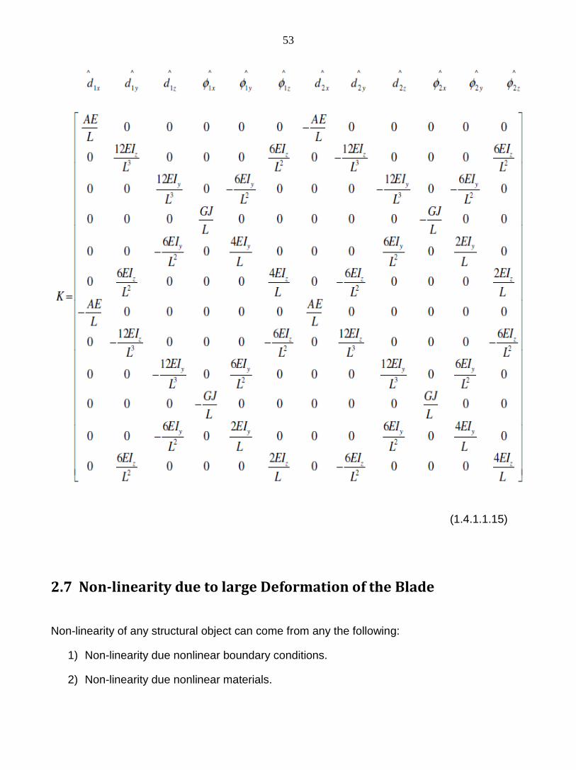
53

(1.4.1.1.15)

2.7 Non-linearity due to large Deformation of the Blade

Non-linearity of any structural object can come from any the following:

1) Non-linearity due nonlinear boundary conditions.

2) Non-linearity due nonlinear materials.

54

3) Non-linearity due nonlinear large deformations. In the present research, the author only considering the nonlinearity due the large

deformation of the blade (displacement exceed 10% of the length of the blade) where the high

order terms of the strain are kept through the derivation of the components of the total strain

energy due the application of all the aerodynamic loadings and their couplings.

This lead to have two additional nonlinear stiffness matrices in the nonlinear dynamic

equation of motion that can be solved for the the six degrees of freedom of displacements at

any x along the length of the blade using the nonlinear Newmark scheme.

2.8 Research Tasks and Plan

2.8.1 Lagrangian Beam Formulation Using the following Lagrangian equations of motion approach:

1) Assuming that deformation is large (where higher order terms of strain are kept through

derivation) and considering all the extensional, torsional and flexural loadings acting on

the blade with their couplings, variable airfoil cross sections with warping effects, shear

deflection, rotary inertia and with blade’s pretwist, the total strain energy, total kinetic

energy and the partial derivatives of the external work external work due to the

aerodynamic loading acting on the blade can be calculated and then substituted in the

Lagrange equations of motion.

2) The “assumed modes method” is used, in which displacements are assumed to be an

expansion of products of time-step dependent constants and polynomial functions of x

(where x is the coordinate along the length of the blade) that satisfy the boundary

55

conditions at the fixed end where x=0 (hub of the blade) and at the free end where x=L

(tip of the blade).

3) Then mass matrix, linear and non linear stiffness matrices and the load vector R of the

dynamic equations of motion are deduced from the Lagrange equations of motion. The

steps of the linear and nonlinear Newmark implicit iteration schemes used for solving

the linear and nonlinear dynamic equations of motion respectively were explained in

detail.

4) To modify the above formulation for the small linear deformation, all what should be

done is to eleminate the higher order terms of the strain that we kept for the large

deformation ( or simply assume the nonlinear stiffness matrices are not exist)

5) Creating a MATLAB code that contain the mathematical formulations that mentioned

above for the linear and nonlinear deformations.

2.8.2 Model Validation

2.8.2.1 Experimental Testing

There will be no experimental testing will be conducted through this present research period

on any wind turbine blade prototype or on a real working wind turbine in the field due to the

difficulty to do that. So to verify my MATLAB code (that contain all the mathematical

formulation of the present research) displacement results after solving for all the unknown

displacements , and in the directions of x, y and z axes respectively, the bending

rotations and about the y and z axes respectively and the torsional rotation about the x

56

axis (using the linear and nonlinear Newmark implicit iteration schemes), the author will

perform the following:

Confirming that the linear case displacement result plots are agree with the work of

Younsi et al.

And confirming that the nonlinear case displacement result plots are agree with the Ls-

Dyna code.

2.8.2.2 Blade Analysis Using Hypermesh and Ls-dyna Consider the 3D blade Fig. 2.8.2.2.1 as an infinite number of stations that each of these

stations has a ‘local radius’, which is the distance of the station from the centre of the rotor.

Fig. 2.8.2.2.1: The Blade stations [11]

Given the local radius, chord width and blade angle at some given number of airfoil stations,

we can construct the shape of the whole blade.

where,

57

chord line: is the longest line within the blade section, and it joins the leading edge to the

trailing edge.

blade pretwist angle (beta): is the angle between the chord line and the plane in which the

rotor spins.

Essential steps to build the given blade Ls-dyna mo del in Hypermesh

Hypermesh, versions10 was used as the finite element preprocessor to model a pretwisted

14 m length wind turbine blade(of linearly decreasing NACA-4415 airfoil type from hub to tip)

and then solve for the blade deformation using Ls-Dyna solver. The following are the essential

steps that used to build the given blade Ls-dyna model in Hypermesh.

1st phase steps: creating the blade model

1) Create a Geom component.

2) Make Geom current and construct all the 1D beam elements using nodes and then lines to

connect the nodes ( 14 1-D beams (total 15 nodes), each beam is 1 m length).

3) Solver Browser then right click ---> create ---> *MAT ---> *MAT _Elastic ---> Create *Mat_

Elastic ( enter the Young’s Modulus E and the poisson ratio of the material).

4) Create properties for each beam section i.e. 14 properties, by entering the associated area

for each beam section as the average of the airfoil areas at the 2 nodes of that beam element

section under consideration---> using a special macro---> enter the coordinates of the average

airfoil as copied from an excel sheet ---> nodes of the airfoil geometry will show on the screen -

--> Go to Geom ---> connect the coordinates of the airfoil geometry--->1D---> Hyperbeam to

create that beam section property). Also using Hyperbeam, any airfoil beam section can be

twisted as shown in the below Fig. 2.8.2.2.1.

58

Fig. 2.8.2.2.2: Airfoil geometrical properties using Hypermesh.

5) Create 14 different 1D_beam sections that all share same material but each has its own

property that created at previous step 4.

6) Meshing: Make the 1st beam element component current then 1D ---> line mesh, then

select the associated property then select the the geometry of the 1st beam then Mesh.

59

7) Create a constraint collector.

8) Make constraint current and select left node and apply constraints at the hub of the blade

(where x=o). Since each 1D_beam section (that created in step 5) has different average airfoil

area, then all the 14 1-D beam elements will change to a 3-D blade as shown in Fig. 2.8.2.2.3.

Fig. 2.8.2.2.3: Changing 1D beams to a 3D blade using Hypermesh.

2nd phase steps: creating the aerodynamic load curv es

1. In the Solver Browser right click and select Create>Set>*Set_Node_List.

2. Name it Node1.

3. Select the first node to be loaded and create the set.

4. Repeat for each node to be loaded. Until you have a Node_Set for each of the nodes.

5. Create your curves for each of the loads you want, X,Y,Z and Rotational X,Y,Z ( view --->

Solver Browser --> *Define ---> create ---> *Define_Curve --> New --> enter X (time) and Y

( load). Then load curves data will looks like Fig. 2.8.2.2.4.

60

Fig. 2.8.2.2.4: The load curves data.

6. In the Solver Browser right click and select Create>Load>*Load_Node_Set.

7. Name it Load1.

8. When the card editor opens click NSID and pick the first node set.

9. Click DOFX and pick 1 (for the x component).

10. Click LCID and pick the curve for the X Load for the first node.

11. Repeat this procedure for the same node_set and pick DOFX 2 (Y Translational) and pick

the LCID for the Y translational load curve.

12. Do this procedure for each node and every DOFX (1,2,3 are X,Y,Z translational and 5,6,7

are X,Y,Z rotational) so that every node has all load curves associated with it.

The final blade model cards are shown in Fig. 2.8.2.2.5.

61

Fig. 2.8.2.2.5: The final blade Ls-Dyna model.

And the final blade model with all the added aerodynamic loadings Fx, Fy, Fz, Mx, My and Mz

at each of the 15 nodes, starting at node1 (where x=0) and ending at node1 (where x=L) are

shown in Fig. 2.8.2.2.6.

62

Fig. 2.8.2.2.6: All stations loadings.

The blade solution of the present research formulation for the linear small deformation case

using the MATLAB code is compared with the same blade solution for the displacements and

rotations plots (six degrees of freedom) at the blade tip with Younsi et al work.

While the blade solution of the present research formulation for the nonlinear large deformation

case using the MATLAB code is compared with the same blade solution for the displacements

and rotations plots (six degrees of freedom) at the blade tip with Ls-Dyna work.

It should be also noted that many other commercial codes have been tried throughout the

present research to generate the geometrical blade properties for some given blade airfoil

stations that linearly decrease from hub to tip as shown in Fig. 1.8.2.2. For example, the new

commercial code VABS (Variational Asymptotical Beam Sectional Analysis) is one of the

codes that can be used to model the wind turbine blade structure for which one dimension is

much larger than the other even if the blade is made of composite materials and have a

63

complex internal structures. Another commercial code is NuMad, one of set of codes created

by NREL that able to create a 3D blade structure from the 2D airfoils. NuMad is a stand-alone,

GUI pre-processor for ANSYS finite element analysis software developed by Daniel Laird at

Sandia National Laboratories. Some other codes like Concord and X-FOIL are used to create

the 2D airfoils from their known coordinates. It should be noted that composite material work

is not the concentration of the present research since that was done before.

2.9 Torsion of Arbitrary Cross-sections

2.9.1 Saint-Venant’s Torsion Theory

It should be noted that for any non circular cross-sections, plane cross-sections will not

remain plane after any torsional deformation and therefore warping of the cross-sections will

occur. This problem of torsion and warping need to resolved in order to predict to a high

accuracy the stress distribution and the deformation of a shaft of any arbitrary cross-sections.

The problem of a cylindrical shaft under torsion was analyzed by Barre de Saint-Venant [12],

who utilized the semi-inverse method (which rely on guessing a part of the solution, then trying

to determine the rest of the solution in a rational way where all the differential equations and

boundary conditions should be satisfied.

Consider a cylindrical shaft under torsion, with the x-axis along its length and with the ends at

x=0 and x=L respectively.

The shear stresses in the cross-sections that perpendicular to the x-axis are:

(2.9.1.1)

where is the given radius vector measured from the central x-axis of the shaft.

J

Tr=τ

r

64

The displacements in the x, y and z directions on the shaft are:

and (2.9.1.2)

where is some function of y and z, called warping function, and is the angle of twist

per unit of length of the shaft and is assumed to be very small (<<1).

The differential equations of equilibrium are:

(2.9.1.3)

where,

ρ : is the density of the substance.

,Xρ : are the body forces (X, Y and Z are the projections on the coordinate axes of the

mass forces (i.e. gravity) acting on each part of the body, relative to the mass of that part.

Relying on the function to satisfy the above differential equilibrium equations and

assuming that the body forces are negligible. The B.C.s on the lateral surface of the shaft are:

=0

(2.9.1.4)

and the B.C.s at the ends x=0 and x=L :

and and are equipollent to the torque (2.9.1.5)

,xzu φ−= v xyφ= ),( zyw φψ=

),( zyψ φ

,Yρ Zρ

),( zyψ

+yyylσ zyzlσ

+yzylσ 0=zzzlσ

+yxylσ 0=zxzlσ

xyσ xzσ T0=xxσ

65

Consider as the direction cosine constants for the lateral surface and ( as the

direction cosine constant for the direction along the shaft length . From Eqn 2.9.1.2 , we can

get the stresses values by using Hooke’s law.

, and

(2.9.1.6)

A substitution of these values into Eqns 2.9.1.3 shows that the equilibrium equations is

satisfied if satisfied Eqn 2.9.1.7 within the cross-section of the cylinder :

(2.9.1.7)

To satisfy the B.C.s, Eqn 2.9.1.4, we should maintain:

on , (2.9.1.8)

where is the boundary of the cross-section of the region R that shown in Fig. 2.9.1.1

.

Fig. 2.9.1.1: An arbitrary cross-section under torsion (adapted from [12]).

but

Therefore the B.C.(s) of Eqn (2.9.1.9) can be written as:

,yl zl )0=xl

),( yz

Gzx +∂∂

=ψ

φσ )( zz

Gxy −∂∂

=ψ

φσ =yzσ =yyσ =zzσ 0=xxσ

),( zyψ

+∂∂

2

2

y

ψ02

2

=∂∂

z

ψ

+−∂∂

),cos()( ylzy

ψ0),cos()( =+

∂∂

zlyz

ψC

C

+∂∂

),cos( lyy

ψ≡

∂∂

),cos( lzz

ψl∂

∂ψ

66

on (2.9.1.9)

The B.C.(s) of Eqn 2.9.1.6

are satisfied if:

and (2.9.1.10)

(2.9.1.11)

We can verify that Eqns. 2.9.1.10 are satisfied if satisfies Eqn 2.9.1.7 and Eqn 2.9.1.9

because:

since satisfies Eqn. 2.9.1.7. By applying the Gauss theorem to the final integral, it

becomes as a line integral on the boundary :

which vanishes on account of Eqn 2.9.1.9. Similarly, the second Eqn of Eqns. 2.9.1.10 must

be satisfied. Finally, the last condition of Eqn. 2.9.1.11 is :

(2.9.1.12)

but (2.9.1.13)

which implies,

(2.9.1.14)

where,

: is the angle of twist at a specific location x along the shaft

: is a proportionality constant or torsional rigidity of the shaft

: is the shear modulus of the shaft

J : is the polar moment of inertia of the shaft cross-section if it is circular.

−=∂

∂),cos( lyz

l

ψ),cos( lzy .C

,0=∫∫ dydzxy

R

σ ,0=∫∫ dydzxz

R

σ

Tdydzzy xyxz

R

=−∫∫ )( σσ

),( zyψ

=∫∫ dydzxy

R

σ dydzzy

GR

)( −∂∂

∫∫ψ

φ [ ]+−∂∂

∂∂

= ∫∫ )( zy

yy

GR

ψφ [ ] ,)( dydzy

zy

z +

∂∂

∂∂ ψ

),( zyψ

C

[ ]dslzylyzl

yGC

),cos(),cos( +−∂

∂∫

ψφ

T φ= dydzy

zz

yzyGR

)( 22

∂∂

−∂

∂++∫∫

ψψ

dydzy

zz

yzyJR

)( 22

∂∂

−∂∂

++= ∫∫ψψ

GJ

G

67

2.9.2 Prandtl Stress Function Theory Prandtl [12] proposed an approach to calculate the warping in which he considers the stress

components as the principal unknowns. Assuming that only and differ from zero, then

all the equations of equilibrium Eqn 2.9.1.3 are satisfied if

(2.9.2.1)

Also Prandtl [12] observes that this equation is identically satisfied if and are derived

from a stress function in such a way that:

and (2.9.2.2)

This stress function can be an arbitrary function as long as the stress system Eqn

2.9.2.2 satisfy the boundary conditions Eqn 2.9.1.4 and Eqn 2.9.2.1 and the compatibility

conditions.

From Eqn 2.9.2.1, we can figure out that the compatibility requires that (in absence of body

forces) the following:

and

where, denotes , hence,

and (2.9.2.3)

(2.9.2.4) Of the boundary conditions Eqn 2.9.1.4 only the last equation is not identically satisfied but

from Fig. 2.9.1.1, we note that:

and (2.9.2.5)

We can write the last equation of Eqn 2.9.1.4 as :

,yxσ zxσ

+∂

∂

yyxσ

0=∂

∂zzxσ

,yxσ zxσ

),( zyϕ

=yxσ ,z∂

∂ϕ−=zxσ

y∂∂ϕ

),( zyϕ

,02 =∇ yxσ ,02 =∇ zxσ 2∇ +∂

∂2

2

(y

)2

2

z∂∂

y∂

∂ 2∇ ,0=ϕz∂

∂ 2∇ 0=ϕ

2∇ .const=ϕ

),cos(ds

dzyll y ==

ds

dyzll z −== ),cos(

68

on (2.9.2.6)

Hence must be constant along the boundary curve For a simply connected region,

it is general enough to set :

on (2.9.2.7)

It remains to examine the boundary conditions Eqn 2.9.1.5. The first,

follows the

starting assumption. The other conditions are stated in Eqns 2.9.1.10 and Eqn 2.9.1.11.

but , by Gauss’ theorem, this is and it vanishes on account

of Eqn 2.9.2.7.

Similarly, the resultant force in z-direction vanishes. Thus Eqn. 2.9.1.10 are satisfied.

Finally, Eqn 2.9.1.11 requires that:

which can be transformed by Gauss’ theorem as follows:

(2.9.2.8)

If R is simply connected region, the line integral vanishes by the boundary conditions Eqn

2.9.2.7, implies: (2.9.2.9)

Thus, all differential equations and boundary conditions concerning stresses are satisfied if

obeys Eqn 2.9.2.6, Eqn 2.9.2.7 and Eqn 2.9.2.8. But there remains an indeterminante

constant in Eqn 2.9.2.6. This constant has to be determined by boundary conditions on

displacements. From Eqn 2.9.1.2 and Eqn 2.9.1.6, we get:

z∂∂ϕ

+∂∂s

z

y∂∂ϕ

=∂∂s

y,0=

∂∂

s

ϕ.C

),( zyϕ .C

,0=ϕ .C

,0=xxσ

=∫∫ dydzxy

R

σ ∫∫R z∂

∂ϕdydz ,dsl z

C

ϕ∫

yyT

R ∂

∂−= ∫∫

ϕ( dydz

zz )

∂

∂+

ϕ

+∂∂

−= ∫∫ )( ϕyy

TR

ϕϕ 2)( −∂

∂z

zdydz

∫−=C

),cos(),cos( zlzyly ϕϕ + dsR∫∫+ dydzϕ2

T dydzR

ϕ∫∫= 2

ϕ

69

and

(2.9.2.10)

Differentiating with respect to z and y, respectively, and subtracting we get:

(2.9.2.11)

Hence, a substitution from (2.9.2.7) gives

(2.9.2.12)

In this way, the problem of torsion is to the solution of the poisson Eqn 2.9.2.12 with boundary

condition Eqn 2.9.2.7.

Elliptical Cross-section Let us apply the Prandtl approach [12] to calculate the warping of an elliptical cross section

where (2.9.2.13)

Then Eqn 2.9.2.12 and Eqn 2.9.2.7 are satisfied by having the stress function:

(2.9.2.14)

Eqn 2.9.2.8 gives the relation between the torque and the rate of twist !

(2.9.2.15)

The stresses are given by Eqn 2.9.2.2. Note the following curves have an interesting meaning:

The slope dz/dy of the tangent to such a curve is determined by the formula:

=∂

∂

y

wz

Gxy α

σ+ =

∂

∂

z

wy

Gxz α

σ−

zGxy

∂

∂σ(

1α

σ2) −=

∂

∂−

yxz

+∂

∂2

2

y

ϕα

ϕG

z2

2

2

−=∂

∂

+2

2

a

y01

2

2

=−b

z

++

−=2

2

22

22

()( a

y

ba

Gba αϕ )1

2

2

−b

z

Gba

baT

)( 22

33

+=

πdx

dφ

),( constzy =ϕ

70

(2.9.2.16)

Hence, according to Eqn 2.9.2.2, we have

and , which implies: .

The magnitude of shearing stress is:

" [ (2.9.2.17)

The maximum shearing stress is :

"

(2.9.2.18)

Now the warping (out of plane displacements) function for a constant elliptic cross-

section can easily be shown to be :

= #$% (2.9.2.19)

where # &'()'&'*)' is a constant depends on the two diameters + and , of the ellipse.

So as mentioned earlier in section 2.9.1, shafts or cylinders of a non-circular cross-section

undergo warping when subjected to pure torsion. An example is the warping that occurs in the

shafts with elliptical cross sections i.e. Eqn 2.9.2.19.

For the present research, warping will be calculated at many selected given stations from hub

to tip of the given wind turbine blade (that has different airfoil dimentions at different cross

sections) where at each selected station there is only a one calculated value of warping that is

different from the next station. Therefore, warping in the present research is considered to be

dependent on x coordinate only and is independent of the y and z coordinates which is

different from the above mentioned constant elliptic cross-section case.

+∂

∂

y

ϕz∂

∂ϕ0=

∂

∂

y

z

=yxσ ,z∂

∂ϕ−=zxσ

y∂∂ϕ

xy

xz

y

z

σσ

=∂∂

(= +2xyσ =2

12 )xzσ +

∂

∂ 2)(y

ϕ2

12 ])(

z∂

∂ϕ

2Gα22

2

ba

ba

+

),( zyψ

=ψ zyba

ba22

22

+

−−

71

2.9.3 Cross-section Geometrical Properties

2.9.3.1 Torsional Rigidity Calculation

The analytical calculation of the exact values of the “torsional rigidity” for cylindrical bars is

limited to a few number of cross-sections. Exact solutions for the ellipse, circle and equilateral

triangle are listed in [13] while the approximations for rectangular cross-sections are available

in [14]. The approximated solution for many cross-sections such as trapezoids, triangle,

semicircles, are listed in handbooks such Roark [15]. A good approach to approximate the

torsional rigidity of any cylindrical solid cross-section is detailed in [15, 16]. Some cross

sections can be considered as a combination of an ellipse, rectangle and triangle, etc.

There are many softwares that can be used to calculate the geometrical properties for any

cross section including warping, moment of inertias and torsional rigidity [16] but for my work I

used the Hypermesh version 10 to calculate such properties that needed for my analysis.

2.9.3.2 Second Moment of Inertia

There are three types of moment of inertia: The second moment of inertia, the product

moment of inertia and the polar moment of inertia. Consider a beam with a cross-sectional

area A (that has a plane region of a particular shape which is perpendicular to the beam's axis).

And consider λ to be a straight line in the plane (which is by definition, perpendicular to the

axis of the beam). The “second moment of area” of the region A about the line λ is:

(2.9.3.2.1) where dA is the elemental area; and n is the perpendicular distance from the element dA to the

line λ

72

If the line λ is the x axis and the bending force is parallel to the y axis, the second moment of

area can be computed as:

(2.9.3.2.2)

To calculate the bending stresses, the above equation can only be used when cross-sections

are symmetrical about the x-axis. But if cross-sections are not symmetrical, the second

moment of area about both the x-axis and y-axis and the product moment of area, Ixy,

(explained in the next section) are required.

2.9.3.3 Product Moment of Inertia

The scalar of the “second moment of area” for a beam about a certain axis, describes the

beam's resistance to bending along that axis. Some beams will deflect in a direction other

than the direction they are loaded. Consider, for example, a leaf spring running along the x

axis and directed such that its surface normal is in the (0,1,1) vector direction. If we push

downward on it in the (0, 0, −1) vector direction, we get a bending moment in the (0,1,0) vector

direction. However, even that the spring is moving downward, it is primarily deflecting in the (0,

−1, −1) vector direction. This behavior should be captured by the “product moment of area”.

The product moment of area is:

(2.9.3.3.1)

where,

x: is the perpendicular distance from y axis to the element dA.

y: is the perpendicular distance from x axis to the element dA.

2.9.3.4 Polar Moment of Inertia

Polar moment of inertia is defined as the quantity that used to predict an object's ability to

resist torsion, in objects with an invariant circular cross

used to calculate the angular displacement of an object when it is subjected to a

analogous to the area moment of inertia that predicts an object's ability to resist bending. The

larger the polar moment of inertia, means the less the beam can twist, when subjected to a

given torque. It should be noted that “polar moment

“moment of inertia”, which characterizes an object's angular acceleration due to a torque.

Limitations

The “polar moment of inertia” can not be utilized to analyze any non

shaft. For non-circular cross-sections shafts, the “torsional constant” should be calculated

instead of the “polar moment of inertia”. In objects with significant cross

(along the axis of the applied torque), which cannot be analyzed in segments, a mo

approach should be used. However the “polar moment of inertia” can be utilized to compute

the “moment of inertia” of an object with arbitrary cross

Fig. 2.9.3.4 A schematic of Fig. 2.9.3.4.1 show how arbitrary shape about an axis o.

73

Polar Moment of Inertia

is defined as the quantity that used to predict an object's ability to

resist torsion, in objects with an invariant circular cross-section and insignificant warping.

used to calculate the angular displacement of an object when it is subjected to a



given torque. It should be noted that “polar moment of inertia” should not be confused with


The “polar moment of inertia” can not be utilized to analyze any non-

sections shafts, the “torsional constant” should be calculated

instead of the “polar moment of inertia”. In objects with significant cross

(along the axis of the applied torque), which cannot be analyzed in segments, a mo


the “moment of inertia” of an object with arbitrary cross-section.

2.9.3.4.1: The polar moment of inertia.

show how the “polar moment of inertia” is calculated for an

.

is defined as the quantity that used to predict an object's ability to

ion and insignificant warping. It is

used to calculate the angular displacement of an object when it is subjected to a torque. It is



of inertia” should not be confused with


-circular cross-section

sections shafts, the “torsional constant” should be calculated

instead of the “polar moment of inertia”. In objects with significant cross-sectional variation

(along the axis of the applied torque), which cannot be analyzed in segments, a more careful


is calculated for an

74

(2.9.3.4.1)

where Jz is the “polar moment of inertia” about the axis z; and ρ is the radial distance to the

element dA from the axis z.

For a circular section with radius r:

(2.9.3.4.2)

For a rectangular section with sides b and h:

(2.9.3.4.3)

The SI unit for the “polar moment of inertia” is the same as the “area moment of inertia” i.e. m4.

Conversion from Area Moment of Inertia

Using the perpendicular axis theorem, the polar moment of inertia Jz is related to the area

moments of inertia about the other two mutually perpendicular axes: Jz = Ix + Iy . The “polar

moment of inertia” Jz appears in the formulae describes torsional stress and angular

displacement.

Torsional stress

(2.9.3.4.4)

where T is the torque; r is the distance from the center; and J z is the polar moment of inertia.

In a circular shaft, the shear stress is maximum at the surface of the shaft where the torque is

maximum:

(2.9.3.4.5)

75

Chapter 3

Total Strain Energy, Total Kinetic Energy, Aerodynamic loadings &

External Work

3.1 Introduction

Wind turbine blades similar to helicopter rotor blades [17] have the structure of pre-twisted

beams that react due to extension, torsion, flexure and the coupling interactions among all

these loads. A number of approximate theories used for the pre-twisted beam have been

developed by different researchers to analyze its complex geometry.

For example, the potential and kinetic energy relationships were given by Carnegie [18] for a

pre-twisted cantilever blade using the standard variational approach to deduce the equations

of motion and allowing for torsion, bending, rotary inertia and deflections due to shear without

any warping effect. Yardimoglu and Yildirim [19] derived the strain energy and kinetic energy

for pretwisted Timoshenko beam undergoing bending-bending load coupling. More recently,

Ozgumus and Kaya derived [20, 21] the strain energy and kinetic energy to obtain the

equations of motion for a rotating beam considering bending-torsional coupling considering the

effect of the centrifugal force and the effect of shear as in a Timoshenku beam. And Liu,

Friend and Yeo [22], derived the strain energy and kinetic energy considering axial-torsional

coupling vibration for a pretwisted beam that has an elliptic cross section. Then they obtained

the equations of motion using Hamilton’s principle assuming an elliptical cross section warping.

The calculation of warping for an eliplitical cross section is elementary and is easy to calculate.

In this chapter, the total strain and total kinetic energy were derived for both the linear small

deformation case and the nonlinear large deformation case.

76

Also the pitch moment, thrust, centrifugal forces (that allow us to obtain the external work

acting on the blade), boundary conditions and damping on the blade will be discussed. It

should be noted that the six unknown displacements at any x along the blade’s length direction

were assumed to be expanded a series of products of time dependent constants and

polynomials expansion and then computed by solving the dynamic equations of motion.

3.2 Dynamic Equations of Motion Consider the blade shown in Fig. 3.2.1 as a Timoshenko beam with a pretwisted angle .

Fig. 3.2.1: Pre-twisted asymmetrical blade structure coordinate systems. The blade has at any x along the lengthwise three displacements u, v and w in the directions

of x, y and z axes respectively, bending rotations and about the y and z axes respectively

and torsional rotation about the x axis. Also we are considering as the airfoil cross

sectional warping.

β

1θ 2θ

φ ψ

77

By applying the following Lagrange equations [23] to the blade of Fig. 3.2.1, we will obtain all

the equations of motion:

0)( .. =

∂

∂−

∂

∂+

∂

∂+

∂

∂+

∂

∂−

∂

∂••

m

ext

mm

sCB

m

Total

mm q

W

q

F

q

U

q

U

q

T

q

T

dt

d (3.2.1)

where,

-.: is equal to +., ,., /., 0., 1. 23 4.

: is the total Kinetic energy

5678&9: is the total strain energy

:;8: is the external work on the blade due to the applied aerodynamic pressure

<: is the applied nonconservative damping force if blade assumed to be of viscous type [61].

where has a different value for each term of the mode expansion. Simple calculation give:

The damping coefficient is related to modal damping ratio, that can be evaluated from

experiments, by where is the natural circular frequency

of mode and is the modal mass of this mode, given by:

In the present research, the author considers only the material damping and neglects the

viscous damping i.e. neglecting the term 0=∂

∂•

mq

F, which results in reducing one term of the

equations 3.2.1 to become:

78

0)( .. =∂

∂−

∂

∂+

∂

∂+

∂

∂−

∂

∂•

m

ext

m

sCB

m

Total

mm q

W

q

U

q

U

q

T

q

T

dt

d (3.2.2)

3.3 Computation of the Total Strain Energy

By adding all the different derived strain energies from Appendix A i.e. equations (A.1), (A.2)

and (A.3), we get the total strain energy [9, 13, 18, 20-22, 24-26]:

=TotalU ( 21θ ′ + 2 + 2

2θ ′ ) + + dx + PL

∫02

1 [ - 2

'v + ))(/( xAI p ] dx + PL

∫02

1 [ - 2 'w + ))(/( xAI p ] dx + E

2

1 dxAw

L4

0

'4

1∫ +

dxwIE p

L22

0

''2

1

2

1φ∫ + + + 2

xxε + 2 G ( 2xyε +

2xzε )

2φ ′′ (3.3)

where,

[ + + + 2)(x

u

∂∂

+ 2)(x∂

∂ψθ + + 2)( ψ

θx∂

∂+

+ + ] where, 2

121

2 zyr +=

(3.3-a)

=xyε θ ][ 1z− and =xzε ][ 1yθ (3.3-b)

3.4 Computation of the Total Kinetic Energy

By adding all the different derived kinetic energies [9, 13, 18, 20, 22, 24-26] from Appendix B

i.e. equations (B.1.2), (B.2) and (B.3), we got the total strain energy as:

EL

∫02

1yyI yzI '1θ '2θ zzI )'(( 1θ−wkGA 2 )'( 2θ−v 2 2v′ αy

'φ 2φ′ 2w′ αz 'φ 2φ ′

[∫L

0 1K '1θ φ′ 2K '2θ φ′ ] dx EdydzA

L

21

0∫∫∫

dx p

L

EI2

1

0∫+ dx

=xxεx

u

∂∂

x∂

∂ψθ ψ

θ

x∂

∂

2

1

2

1

x

u

∂∂

x∂

∂ψθ

2

1

x∂

∂ψθ ψ

θ

x∂

∂

x

u

∂∂

ψθ

x∂

∂

2

12r θ 2

2

1

2

1

79

=T +•

)(2

xAu )(xA + 2)(x∂

∂•

φ)(xA + ]dxxI p

2

)(•

φ

422222

2222222

22

0

)(4

1)()()()(

2

1φφθφθρ xAyxAzxAyxAzx

L

Ω+Ω−Ω−Ω+ ∫ 22 )( uxAΩ+•

Ω+ 222 )(2 θφxAy 2

2 )(2•

Ω− θφxAz

+Ω+•

232 )( θφxAz )(2 xAz 2

2

•

θ 22

22 )(•

− θφxAz•

Ω+ φθ22 )(2 xAy )(2 2 xAzΩ+

••

Ω− φφθφθ 22

22 )(xAy 2zΩ−

)(xA +•

φφθ 22

••

φθφθ 222 )(2 xAy

••

− φθφθ 222 )(2 xAz )(2 xAy+

22

2

)(••

+ φφ xAz dxxAy2

22

2 )(•

+ φθ

[ ]dxywzvxmL

22

0

)()()(2

1 ••••

++++ ∫ φφ αα zz

L

Ix)(2

1

0

ρ∫+ yyIx)(ρ+ dx

[ 2

0

2

)''()(2

φαzvxmL

+Ω

− ∫ ++ '(w 2)'φαy ]xdx +

(3.4)

3.5 Displacement Expansion

The author assumed a summation of a product of time dependent constants and polynomials

expansion for the three displacements =, , and the three rotations at any x along the

blade length as shown below in order to solve for them using the Assumed Modes Method:

similarly,

and

(3.5)

where the polynomial functions and and are the

time dependent constants that need to be solved using the equations of motion and Newmark

non-linear iteration scheme.

[)(2

1

0

xL

ρ∫•

u2 )(

•

∂∂x

φ ψ2ψ

22 )(

••

′+ φθ αz2

1 )( φθ αy −′+••

[g

zzxI zzL 2

2

0

))((

2

1•• ′+′+

∫φφθρ αα

] dxg

yyxI yy2

1 ))((•• ′+′+

+φφθρ αα

φθθ ,, 21

),()(1

xtau nn

N

n

φ∑=

=

),()(1

xtbv nn

N

n

φ∑=

= ),()(1

xtcw nn

N

n

φ∑=

= ),()(1

1 xtd nn

N

n

φθ ∑=

= )(1

2 ten

N

n

φθ ∑=

= ),(xnφ

)()(1

xtf nn

N

n

φφ ∑=

=

1)/()( += nn Lxxφ )(),(),(),(),( tetdtctbta nnnnn )(tfn

80

3.6 Thrusts, torques, centrifugal forces and pitch moments True distributions of the aerodynamic loadings that needed for the structural analysis of the

wind turbine blades, are difficult to predict and usually require some flow codes such as CFD

to determine their accurate magnitude. In this section I am providing a simple model for the

estimate of blade forces suitable for use in structural analysis. Thrust forces are directed in the

axial direction (i.e., following the blade shaft axis). Torque forces are tangent to the radius arc.

Centrifugal forces are normal to the axis. As noted earlier that according to the BEM theory

[27], air loads on a section airfoil of the blade are proportional to the dynamic pressure at only

that section.

The premise of the simplified model is that a) the forces can be modeled by a set of point

loads rather than distributed pressures, and b) the magnitudes of these point loads can be

estimated using the below load formulaes, c) An interpolation scheme needed to have all

computed forces and moments as a function of the blade lengthwise x. Fig. 3.6.1 below,

illustrates how the three principal forces - thrust, torque and centrifugal- are applied as point

loads acting on a radial span of the blade.

The aerodynamic forces (lift, drag and pitching moment) as shown in Fig. 3.6.1 are directly

linked to the type of flow, relative wind velocities and the wind attack angles to the airfoil

sections.

Lift: L = ρ >;9 / 9

Drag: D = ρ >;9 /

Pitch Moment: ?@ = ρ >;9 / . (3.6.1)

The simplified model is stating that (a) the forces can be modeled by a set of station loads

rather than distributed loads, and (b) then the magnitudes of these station loads can be

81

predicted using the below listed load formulas, (c) then an interpolation scheme will interpolate

all computed station loads (forces and moments) as a function of the blade lengthwise x.

Fig. 3.6.1: The lift and drag forces.

Fig. 3.6.2 below, illustrates how the three principal forces - thrust, torque and centrifugal- are

applied as point loads acting on a radial span of the blade. Thrust forces are always axial in

their direction (i.e., following the blade shaft axis). Torque forces will be tangent to the radius

arc and centrifugal forces are normal to the axis.

Then all the forces and moments acting at the selected airfoil stations along the blade can be

calculated from the following formulaes [28-30]:

Centrifugal force: Fx = m 3 Ω

Torque force: Fy = L sin − D cos

Thrust force: Fz = L cos + D sin

Moment in x-direction: Mx = ?@ + Fy + Fz (3.6.2)

αz αy

82

Fig. 3.6.2: The aerodynamic loads (adapted from [27]).

where,

9 , and . : are the lift, drag and pitch moment coefficients respectively

φ : is flow angle of the airfoil section

: is the density of the air

/ : is the chord length of the airfoil section

m : is the mass of the airfoil section

>;9 (or :) : is the wind relative speed

Ω : is angular speed of rotor

3 : is the distance from root of the blade to the airfoil section

and : are the distance between centre-of-flexure and centroid in y and z direction

respectively for a specific airfoil section

3.7 External Work The work done by external forces [23, 27, 31] on the blade is:

(3.7.1)

αy αz

dxxMxMxMwxFvxFuxFW zyxzyx

L

ext ])()()()()()([ 21

0

θθφ +++++= ∫

83

where,

, and : are the interpolated functions at all stations of the forces at each time

step acting in the direction of and axes respectively.

, and are the interpolated functions at all stations of the moments at

each time step acting in the direction of and axes respectively.

similarly,

(3.7.2)

(3.7.3)

(3.7.4)

(3.7.5)

(3.7.6)

3.8 Boundary Conditions

The blade strain energy due to the boundary conditions at x=0 and x=L:

)(xFx )(xFy )(xFz

yx, z

)(xM x )(xM y )(xM z

yx, z

=∂

∂

m

ext

a

W)(

0

xFa

x

L

m

∑∫∂

∂),()(

1

xta nn

N

n

φ∑=

dx )()(0

xxF mx

L

φ∫= dx

=∂

∂

m

ext

b

W)()(

0

xxF my

L

φ∫ dx

=∂

∂

m

ext

c

W)()(

0

xxF mz

L

φ∫ dx

=∂

∂

m

ext

d

W)()(

0

xxM my

L

φ∫ dx

=∂

∂

m

ext

e

W)()(

0

xxM mz

L

φ∫ dx

=∂

∂

m

ext

f

W)()(

0

xxM mx

L

φ∫ dx

2..1.... CBCBsCB UUU +=

84

where ( , , , , , ) and ( , , , , , , ) are the linear and

rotational spring stiffnesses at and respectively.

( + ) +

Considering the polynomials as mentioned in section 3.5, implies:

and , implies:

(3.8)

Similarly, for , , , and

Since the blade has a fixed end at x=0 and a free end at x=L, we can set up the following:

, , and , , to large number and , , and , , to zero or

very small number.

)(2

1)(

2

1)(

2

1)(

2

1)(

2

1)(

2

1

)0(2

1)0(

2

1)0(

2

1)0(

2

1)0(

2

1)0(

2

1

22

21

2222

220

210

20

20

20

20

21

21

LKLKLKLwkLvkLuk

KKKwkvkuk

llllwlvul

wvu

θθφ

θθφ

θθφ

θθφ

++++++

+++++=

uk0 vk0 wk0 ulk lvk lwk φ0K10θK 20θK φlK

1θlK 2θlK

0=x Lx =

=∂

∂

m

sCB

a

U ..

ma∂

∂)0(

2

1 20 uk u )(

2

1 2 Luk ul = )0(0 uk u

ma∂

∂)0(u )(Luk ul

ma∂

∂)(Lu

1)/()( += nn Lxxφ

0)0( =u =)(Lu n

N

n

a∑=1

m

sCB

a

U

∂

∂ .. = k ul n

N

n

a∑=1

m

sCB

b

U

∂

∂ ..

m

sCB

c

U

∂

∂ ..

m

sCB

d

U

∂

∂ ..

m

sCB

e

U

∂

∂ ..

m

sCB

f

U

∂

∂ ..

uk0 vk0 wk0 φ0K10θK 20θK ulk lvk lwk φlK

1θlK 2θlK

85

Chapter 4

Obtaining the Lagrange Equations of Motion

4.1 Introduction A carefully selected sample of the pretwisted beam or wind turbine blade literature is

analyzed, such as the exact solutions of Timoshenko’s equation for simply supported uniform

beams as given by Anderson [32], and the general equations of motion of a pre-twisted

cantilever blade derived by Carnegie [33]. Carnegie [18] extended the study of the general

equations of motion of a pre-twisted cantilever blade allowing for torsion, bending, rotary inertia

and deflections due to shear but he did not include the warping effect. Dawson et al. [34]

found the natural frequencies of pre-twisted cantilever beams of uniform rectangular cross-

section allowing for shear deformation and rotary inertia by the numerical integration of a set of

first-order simultaneous differential equations. Carnegie and Thomas [35] investigated the

effects of shear deformation and rotary inertia on the frequencies of flexural vibration of pre-

twisted uniform and tapered cantilever beams by using the finite-difference method. The semi-

inverse method was proposed by Saint Venant for solving the elastic deformation of prismatic

rods under resultant end loadings. This was referenced and utilized by Dawson, Ghosh, and

Carnegie [34], Xu, Zhong and Zhang [12], and Sokolnikoff [13]. The strain energy of bending-

torsional and their coupling were investigated by Kima, Fub and Kimc [36] and was modified to

include the shear effect of a Timoshenku beam by Kaya and Ozgumus [20]. Banerjee [37, 38]

had an approach for the Bernoulli and another one for the Timoshenko symmetric beam where

bending was uncoupled from torsion and/or axial loading. Banerjee and Williams [39]

published some work about coupled torsional–bending for asymmetrical Timoshenko beam

where the elastic mass axis is different from the centroid axis. Subrahmanyam, Kulkarni and

Rao worked on coupled bending-bending vibrations of pretwisted cantilever blade [40, 41], and

86

also they worked on coupled bending-torsion vibrations of rotating blades of asymmetric

aerofoil cross section with allowance for shear deflection and rotary inertia by use of the

Reissner method [24].

The equations of motion for thin-walled beam with non-symmetric cross-section subjected to

linearly variable axial force were derived by Kim, Fub and Kim [36]. Also one of these early

approximate approaches was Chu’s helical fiber assumption [42], where stresses are initially

determined along and perpendicular to helical fibers of the beam’s pretwist. Even though Chu’s

predictions matched experimental results for thin-walled beams, it was nevertheless a flawed

theory that predicted axial–torsional coupling where warping wasn’t present i.e. for the case of

beams with circular cross-sections. Similar approahes include the works of Rosen [43, 44],

Hodges [45], Krenk [46] on static axial–torsional coupling and Tsuiji [47] on the dynamic

response. In recent years, warping function-based beam theories that based on semi inverse

and variational methods appear to have become widely accepted. The semi-inverse method

was proposed by Saint Venant for solving the elastic deformation of prismatic rods under

resultant force and moment end loads [12, 13, 34].

More recently, Liu, James and Yeo [22], investigated the coupled axial–torsional vibration of

pretwisted beams of elliptic cross section. The equations of motion governing the extension,

torsion, and cross-sectional warping of pretwisted beams were derived from Hamilton’s

principle.

The calculation of warping for an eliplitical cross section is elementary and is easy to calculate.

Younsi et al. [28] used a finite element approach based on a variational formulation of the

theory of beams to calculate the blade tip vertical displacement for a 14m untwisted blade of a

variable NACA 4415 type airfoil. Younsi et al. interpolated the forces and moments for a given

wind velocity and attack angle, for all points of the lift line along the blade using a parametric

method based on Bézier surfaces.

87

In the present research, the author study the linear deformation of a wind turbine blade of the

same characteristics of the blade that was considered by Younsi et al. [28] (i.e. 14m untwisted

blade of a variable NACA 4415 type airfoil) assuming the effect of all the extensional, torsional

and flexural loadings with all their couplings, shear deflection, rotary inertia, warping of the

airfoil cross-section that varies linearly from hub to tip. The strain and kinetic energies were

derived to obtain the dynamic equations of motion that were solved to compute the

displacemts and rotations at many stations along the blade length using the linear Newmark

iteration scheme that will be discussed in more detail in section 6.4 .

Then the author extend his work to include the nonlinear large deformation case which

creates two additional nonlinear stiffness matrices. Also the blade’s pretwist is included. Then

the nonlinear dynamic equations of motion are solved for the three unknown displacements in

the directions of x, y and z axes and the three unknown rotations about the x, y and z axes at

the required stations along the lengthwise of the given blade using the nonlinear Newmark

iteration scheme that will be discussed in more detail in section 6.6 .

4.2 Derivation of the Lagrange Equations of Motion Using Eq. (3.2.2) for -. +. :

0)( .. =∂

∂−

∂

∂+

∂

∂+

∂

∂−

∂

∂•

m

ext

m

sCB

m

Total

mm a

W

a

U

a

U

a

T

a

T

dt

d

Substituting for dxxxFa

Wmx

L

m

ext )()(0

φ∫=∂

∂,

0.. =∂

∂

m

sCB

a

U

(since given polynomial functions

that discussed in section 2.3 satisfy the B.C.s), m

Total

a

U

∂∂

, and

(that was derived in Appendix C and D), implies,

1)/()( += nn Lxxφ

∂

∂• )(

ma

T

dt

d

∂

∂

ma

T

88

=∂

∂−

∂

∂+

∂

∂+

∂

∂−

∂

∂•

m

ext

m

sCB

m

Total

mm a

W

a

U

a

U

a

T

a

T

dt

d ..)( −

+

+ +

+

+ +

+ +

+ +

+

+

+

(4.2-a)

Amn

N

n

s∑=

=1

ρ••

na + ρ ∑=

N

n 1mnDs

1′

••

nfN

n∑

=

Ω1

2ρ nAmnas + E

∑=

N

n 1AmnS na ∑

=

+N

n

E1

mnDS5 nf ∑

=

+N

n

E1

mnDS1

' nf 2

1+ E ∑∑

==

K

k

N

n 11AmnkS knaa

2

1+ E ∑∑

==

K

k

N

n 11mnkDS

6

kn ff E ∑∑==

K

k

N

n 11mnkDS

5 knaf2

1+ E ∑∑

==

K

k

N

n 11mnkDS

2'' kn ff + E ∑∑

==

K

k

N

n 11mnkDS

9' kn ff + E

∑∑==

K

k

N

n 11mnkDS

1' knaf

2

1+ E ∑∑

==

K

k

N

n 11mnkI p

S kn ff + E ∑∑==

K

k

N

n 11AmnkS knaa E ∑∑

==

K

k

N

n 11mnkDS

5 knaf E

∑=

N

n 1∑

=

K

k 1mnkDS

1' knaf

2

1+ E ∑∑

==

LK

lk

N

n

,

1,1AmnklS lkn aaa

2

1+ E ∑∑

==

LK

lk

N

n

,

1,1mnklDS

6 lkn aff E ∑∑==

LK

lk

N

n

,

1,1

mnklDS5 lkn aaf

2

1+ E ∑∑

==

LK

lk

N

n

,

1,1mnklDS

2'' lkn aff E ∑∑

==

LK

lk

N

n

,

1,1mnklDS

9' lkn aff E ∑∑

==

LK

lk

N

n

,

1,1mnklDS

1'

lkn aaf2

1+ E ∑∑

==

LK

lk

N

n

,

1,1mnklI p

S lkn aff E ∑∑==

K

k

N

n 11mnkDS

5 knaf E ∑∑==

K

k

N

n 11mnkDS

6 kn ff + E

∑∑==

K

k

N

n 11mnkDS

9' kn ff

21

+ E ∑∑==

LK

lk

N

n

,

1,1mnklDS

5 lkn aaf21

+ E ∑∑==

LK

lk

N

n

,

1,1mnklDS

7 lkn fff + E ∑∑==

LK

lk

N

n

,

1,1

mnklDS6 lkn aff

21

+ E ∑∑==

LK

lk

N

n

,

1,1mnklDS

10'' lkn fff E ∑∑

==

LK

lk

N

n

,

1,1mnklDS

22' lkn fff E ∑∑

==

LK

lk

N

n

,

1,1mnklDS

9'

lkn aff21

+ E ∑∑==

LK

lk

N

n

,

1,1mnklDS

12 lkn fff + E ∑∑==

K

k

N

n 11mnkDS

1' knaf + E ∑∑

==

K

k

N

n 11mnkDS

9' kn ff + E

∑∑==

K

k

N

n 11mnkDS

2'' kn ff

21

+ E ∑∑==

LK

lk

N

n

,

1,1mnklDS

1' lkn aaf

21

+ E ∑∑==

LK

lk

N

n

,

1,1mnklDS


==

LK

lk

N

n

,

1,1

mnklDS9

' lkn aff21

+ E ∑∑==

LK

lk

N

n

,

1,1mnklDS

3''' lkn fff E ∑∑

==

LK

lk

N

n

,

1,1mnklDS


==

LK

lk

N

n

,

1,1mnklDS

2''

lkn aff21

+ E ∑∑==

LK

lk

N

n

,

1,1mnklDS

28' lkn fff )()(

0

xxF mx

L

φ∫− 0=dx

89

Similarly, by using Eqn (3.2.2) for -. ,., /., 0., 1., and 4., we obtain the following

equations (4.2-b), (4.2-c), (4.2-d), (4.2-e) and (4.2-f) respectively:

=∂

∂−

∂

∂+

∂

∂+

∂

∂−

∂

∂•

m

ext

m

sCB

m

Total

mm b

W

b

U

b

U

b

T

b

T

dt

d ..)( + +

+

(4.2-b)

=∂

∂−

∂

∂+

∂

∂+

∂

∂−

∂

∂•

m

ext

m

sCB

m

Total

mm c

W

c

U

c

U

c

T

c

T

dt

d ..)( + +

+

(4.2-c)

=∂

∂−

∂

∂+

∂

∂+

∂

∂−

∂

∂•

m

ext

m

sCB

m

Total

mm d

W

d

U

d

U

d

T

d

T

dt

d ..)(g

ρ− ∑

=

N

n 1mnI y

s

g

ρ− ∑

=

N

n 1

mnIy ys

α'

g

ρ− ∑

=

N

n 1mnIy y

s 'α+ +

(4.2-d)

=∂

∂−

∂

∂+

∂

∂+

∂

∂−

∂

∂•

m

ext

m

sCB

m

Total

mm e

W

e

U

e

U

e

T

e

T

dt

d ..)(

••

=

••

=∑∑ + nAmnz

N

nnAmn

N

n

fsbsα

ρρ11

nxAmn

N

n

bSρ∑=

Ω−1

2

nAmnxz

N

n

fSα

ρ∑=

Ω1

2 kG ∑=

N

n 1AmnS nb kG− ∑

=

N

n 1Amns' ne + ∑

=

N

n 1PmnS nb − ∑

=

N

n 1mnPyS

α nf

0)()(0

=− ∫ dxxxF my

L

φ

••

=

••

=∑∑ + nAmny

N

nnAmn

N

n

fscsα

ρρ11

ρΩ2nxAmn

N

n

cS∑=1

nAmnxy

N

n

fSα

ρ∑=

Ω1

2 kG ∑=

N

n 1AmnS nc kG− ∑

=

N

n 1Amns' nd + ∑

=

N

n 1PmnS nc − ∑

=

N

n 1mnPzS

α nf 21

+ E

∑∑==

LK

lk

N

n

,

1,1lknAmnkl cccS

21

+ E ∑∑==

LK

lk

N

n

,

1,1lknmnklI ffcS

p0)()(

0

=− ∫ dxxxF mz

L

φ

••

=

••

=∑∑ + nmnyI

N

nnmnI

N

n

fsdsyy α

ρρ '11

nd

•

nf•

nf E ∑=

N

n 1mnI y

S nd E ∑=

N

n 1mnI yz

S ne kG− ∑=

N

n 1Amns' nc kG+ ∑

=

N

n 1Amns

nd + ∑=

N

n 1mnKS

1 nf )()(0

xxM my

L

φ∫− 0=dx

•

=∑Ω− nmnI

N

n

fsz

1

ρ•

=∑Ω− nmnI

N

n

fsy

1

ρLK

lk

N

n ==∑∑Ω+

,

1,1

ρ mnklIsy

lkn fff•

lknmnklI

LK

lk

N

n

fffsy

•

==∑∑Ω+

,

1,1

ρ•

==∑∑Ω+ lknmnklI

LK

lk

N

n

fffsy

,

1,1

ρ••

=∑+ nmnI

N

n

esy

1

ρ==

∑∑−LK

lk

N

n

,

1,1

ρ mnklIsy

90

− + −

− + +

+ − − −

+ +

=0 (4.2-e)

=∂

∂−

∂

∂+

∂

∂+

∂

∂−

∂

∂•

m

ext

m

sCB

m

Total

mm f

W

f

U

f

U

f

T

f

T

dt

d ..)(

••

lkn eff••

==∑∑− lknmnklI

LK

lk

N

n

effsy

,

1,1

ρ••


LK

lk

N

n

effsy

,

1,1

ρ••

==∑∑+ lknmnklI

LK

lk

N

n

ffesz

,

1,1

ρ==

∑∑+LK

lk

N

n

,

1,1

ρ

••

lknmnklI ffesz

••

==∑∑+ lknmnklI

LK

lk

N

n

ffesz

,

1,1

ρ==

∑∑−LK

lk

N

n

,

1,1

ρ••

lknmnklI ffesy

==∑∑− mnklI

LK

lk

N

n

sy

,

1,1

ρ••

lkn ffe==

∑∑−LK

lk

N

n

,

1,1

ρ

••

lknmnklI ffesy

••

=∑+ nmnI

N

n

esz

1

ρ••

=∑+ nmnzI

N

n

fsz α

ρ '1

nmnI

N

n

esy∑

=

Ω1

2ρN

n∑

=

Ω1

2ρLK

lk∑

=

,

1,mnklI fs

y lkn effN

n∑

=

Ω+1

ρ

mnI zs

•

nf•

=∑Ω nmnI

N

n

fsy

1

ρ•

==∑∑Ω lknmnklI

LK

lk

N

n

fffsz

,

1,121

ρ ρΩ2

1

=∑

N

n 1

•

=∑ lknmnklI

LK

lk

fffsy

,

1, ==∑∑−

LK

lk

N

n

,

1,1

ρ

••

lknmnklI fefsz

ρ••

==∑∑ lknmnklI

LK

lk

N

n

fefsy

,

1,1 ==∑∑ mnklI

LK

lk

N

n

sz

,

1,1

ρ ne•

kf•

lfg

ρmnI

N

nz

s∑=1

neg

ρ

••

′==

∑∑ knmnkzzI

K

k

N

n

ffsz αα

'11

E ∑=

N

n 1mnI z

S ne E ∑=

N

n 1mnI yz

S nd kG− ∑=

N

n 1Amns' nb kG+ ∑

=

N

n 1Amns ne + ∑

=

N

n 1

mnKS2 nf )()(

0

xxM mz

L

φ∫− dx

••

=∑ nmnD

N

n

as1

'1

ρ••

=∑+ nmnD

N

n

fS2

1

ρ••

=∑+ nmnI

N

n

fsp

1

ρ=

∑Ω+N

n 1

ρ

•

nmnI esz

•

=∑Ω+ nmnI

N

n

esy

1

ρ lknmnklI

LK

lk

N

n

ffesz

•

==∑∑Ω−

,

1,1

LK

lk

N

n ==∑∑Ω−

,

1,1lknmnklI ffes

z

• N

n=∑Ω−

1

LK

lk =∑

,

1,

•

lknmnklI ffesz

lknmnklI

LK

lk

N

n

ffesy

•

==∑∑Ω−

,

1,12

1ρ

LK

lk

N

n ==∑∑Ω−

,

1,12

1ρ lknmnklI ffes

y

•

==∑∑Ω−

LK

lk

N

n

,

1,12

1ρ mnklIs

y

•

lkn ffe==

∑∑+LK

lk

N

n

,

1,1

ρ

••

lknmnklI efesz

••

==∑∑+ lknmnklI

LK

lk

N

n

efesz

,

1,1

ρ••

==∑∑+ lknmnklI

LK

lk

N

n

efesz

,

1,1

ρ==

∑∑− mnklI

LK

lk

N

n

sy

,

1,1

ρ••

lkn efe==

∑∑−LK

lk

N

n

,

1,1

ρ

••

lknmnklI efesy

==∑∑−

LK

lk

N

n

,

1,1

ρ••

lknmnklI efesy

••

=∑+ nmnI

N

n

fsz

1

ρ••

=∑+ nmnI

N

n

fsy

1

ρ==

∑∑+LK

lk

N

n

,

1,1

ρ mnklIsz

••

lkn fee

==∑∑+ mnklI

LK

lk

N

n

sz

,

1,1

ρ••

lkn fee••

==∑∑+ lknmnklI

LK

lk

N

n

feesz

,

1,1

ρ••

=∑+ nmnMz

N

n

bsα

1

••

=∑+ nmnMz

N

n

fs 2

1α

=∑+ mnMy

N

n

sα

1

••

nc

91

+ + −

− + − + +

+ − +

mnxMz

N

n

Sα∑

=

Ω+1

2nb nmnxMz

N

n

fS 2

1

2

α∑

=

Ω+ nmnxMy

N

n

cSα∑

=

Ω+1

2nmnxMy

N

n

fS 2

1

2

α∑

=

Ω+

+

••

=∑+ nmnMy

N

n

fs 2

1α

••

=∑+ nmnzI

N

n

esz α

ρ '1 =

∑+mnzI

N

n

Sz

2

1α

ρ••

nf••

=∑+ nmnyI

N

n

dsy α

ρ '1

••

=∑+ nmnyI

N

n

fSy

2

1α

ρ=

∑+N

ng

ρ

1

•

nmnzI esz α

'•

′=

∑+ nmnzI

N

n

esg z α

ρ

1

••

=∑+ nmnzI

N

n

fSg z

2

1α

ρ ••

′=

∑+ nmnzI

N

n

fsg z

2

1 α

ρ •

=∑+ nmnyI

N

n

dsg y α

ρ'

1

•

′=

∑+ nmnyI

N

n

dsg y α

ρ

1

••

=∑+ nmnyI

N

n

fSg y

2

1α

ρ ••

′=

∑+ nmnyI

N

n

fsg y

2

1 α

ρΩ2ρ nmnI

N

n

fsz∑

=1lknmnklI

LK

lk

N

n

feesy∑∑

==

Ω,

1,1

2ρLK

lk

N

n∑∑

==

Ω,

1,1

2

2

1ρ

lknmnklI fffsz

•

=∑Ω nmnI

N

n

esz

1

ρ Ωρ•

=∑ nmnI

N

n

esy

1

•


LK

lk

N

n

effsy

,

1,12

3ρ

==∑∑ mnklI

LK

lk

N

n

sy

,

1,1

ρ••

lkn eef

mnklI

LK

lk

N

nz

s∑∑==

Ω,

1,1

ρ lkn ffe•

lknmnklI

LK

lk

N

n

ffesy

•

==∑∑Ω

,

1,1

ρ••

==∑∑ lknmnklI

LK

lk

N

n

feesz

,

1,1

ρ==

∑∑ mnklI

LK

lk

N

n

sy

,

1,1

ρ•

kn ee•

lf

− ∑=

N

n 1mnPyS

α nb ∑=

+N

n 1

2

mnAPI pS )/( nf ∑

=

−N

n 1mnPzS

α nc mnklI

LK

lk

N

np

SE ∑∑==

,

1,12

1lkn fcc ∑

=

+N

n 1mnKS

1 nd ∑=

+N

n 1mnKS

2 ne + E ∑=

N

n 1mnDS

5

na + E ∑=

N

n 1mnDS

6 nf + E ∑=

N

n 1mnDS

9' nf 2

1+ E ∑∑

==

K

k

N

n 11mnkDS

5 knaa21

+ E ∑∑==

K

k

N

n 11mnkDS

7 kn ff +

E ∑∑==

K

k

N

n 11mnkDS

6 kn fa21

+ E ∑∑==

K

k

N

n 11mnkDS

10'' kn ff + E ∑∑

==

K

k

N

n 11mnkDS

22' kn ff + E ∑∑

==

K

k

N

n 11mnkDS

9'

kn fa21

+ E ∑−=

N

n 4∑

−=

K

k 4mnkDS

12 kn ff + E ∑=

N

n 1mnDS

1' na + E ∑

=

N

n 1mnDS

9' nf + E ∑

=

N

n 1mnDS

2'' nf 2

1+

E ∑∑==

K

k

N

n 11mnkDS

1' knaa

21

+ E ∑∑==

K

k

N

n 11mnkDS

22' kn ff + E ∑∑

==

K

k

N

n 11mnkDS

9' kn fa

21

+ E ∑∑==

K

k

N

n 11

mnkDS3

''' kn ff + E ∑∑==

K

k

N

n 11mnkDS

10'' kn ff + E ∑∑

==

K

k

N

n 11mnkDS

2'' kn fa

21

+ E ∑∑==

K

k

N

n 11mnkDS

28' kn ff

+ E ∑∑==

K

k

N

n 11mnkDS

6 kn fa + E ∑∑==

K

k

N

n 11mnkDS

7 kn ff + E ∑∑==

K

k

N

n 11mnkDS

22' kn ff

21

+ E ∑∑==

LK

lk

N

n

,

1,1

mnklDS6 lkn faa

21

+ E ∑∑==

LK

lk

N

n

,

1,1mnklDS

8 lkn fff + E ∑∑==

LK

lk

N

n

,

1,1mnklDS

7 lkn ffa21

+ E ∑∑==

LK

lk

N

n

,

1,1mnklDS

23''

92

lkn fff + E ∑∑==

LK

lk

N

n

,

1,1mnklDS

24' lkn fff + E ∑∑

==

LK

lk

N

n

,

1,1mnklDS

22' lkn ffa

21

+ E ∑∑==

LK

lk

N

n

,

1,1mnklDS

30 lkn fff

+ E ∑∑==

K

k

N

n 11mnkDS

5 knaa + E ∑∑==

K

k

N

n 11mnkDS

6 kn fa + E ∑∑==

K

k

N

n 11mnkDS

9' kn fa

21

+ E ∑∑==

LK

lk

N

n

,

1,1

mnklDS5 lkn aaa

21

+ E ∑∑==

LK

lk

N

n

,

1,1mnklDS

7 lkn ffa + E ∑∑==

LK

lk

N

n

,

1,1mnklDS

6 lkn faa21

+ E ∑∑==

LK

lk

N

n

,

1,1mnklDS

10''

lkn ffa + E ∑∑==

LK

lk

N

n

,

1,1mnklDS

22' lkn ffa + E ∑∑

==

LK

lk

N

n

,

1,1mnklDS

9' lkn faa

21

+ E ∑∑==

LK

lk

N

n

,

1,1mnklDS

12 lkn ffa +

E ∑∑==

K

k

N

n 11mnkDS

2 kn fa + E ∑∑==

K

k

N

n 11mnkDS

10'' kn ff + E ∑∑

==

K

k

N

n 11mnkDS

3''' kn ff

21

+ E ∑∑==

LK

lk

N

n

,

1,1mnklDS

2''

lkn faa21

+ E ∑∑==

LK

lk

N

n

,

1,1mnklDS

23'' lkn fff + E ∑∑

==

LK

lk

N

n

,

1,1mnklDS

10'' lkn ffa

21

+ E ∑∑==

LK

lk

N

n

,

1,1mnklDS

4''''


LK

lk

N

n

,

1,1mnklDS

25''' lkn fff + E ∑∑

==

LK

lk

N

n

,

1,1mnklDS

3''' lkn ffa

21

+ E ∑∑==

LK

lk

N

n

,

1,1mnklDS

29'' lkn fff

+ E ∑∑==

K

k

N

n 11mnkDS

9' kn fa + E ∑∑

==

K

k

N

n 11mnkDS

22' kn ff + E ∑∑

==

K

k

N

n 11mnkDS

10'' kn ff

21

+ E ∑∑==

LK

lk

N

n

,

1,1mnklDS

9'

lkn faa21

+ E ∑∑==

LK

lk

N

n

,

1,1mnklDS

24' lkn fff + E ∑∑

==

LK

lk

N

n

,

1,1mnklDS

22' lkn ffa

21

+ E ∑∑==

LK

lk

N

n

,

1,1mnklDS

25'''


LK

lk

N

n

,

1,1mnklDS

23'' lkn fff + E ∑∑

==

LK

lk

N

n

,

1,1mnklDS

10'' lkn ffa

21

+ E ∑∑==

LK

lk

N

n

,

1,1mnklDS

11' lkn fff

+ E ∑∑==

K

k

N

n 11mnkDS

9' kn fa + E ∑∑

==

K

k

N

n 11mnkDS

22' kn ff + E ∑∑

==

K

k

N

n 11mnkDS

10'' kn ff

21

+ E ∑∑==

LK

lk

N

n

,

1,1mnklDS

9'

lkn faa21

+ E ∑∑==

LK

lk

N

n

,

1,1mnklDS

24' lkn fff + E ∑∑

==

LK

lk

N

n

,

1,1mnklDS

22' lkn ffa

21

+ E ∑∑==

LK

lk

N

n

,

1,1mnklDS

25'''


LK

lk

N

n

,

1,1mnklDS

23'' lkn fff + E ∑∑

==

LK

lk

N

n

,

1,1mnklDS

10'' lkn ffa

21

+ E ∑∑==

LK

lk

N

n

,

1,1mnklDS

11' lkn fff

+ E ∑∑==

K

k

N

n 11mnkDS

1' knaa + E ∑∑

==

K

k

N

n 11mnkDS

9' kn fa + E ∑

=

N

n 1∑

=

K

k 1mnkDS

2'' kn fa

21

+ E ∑∑==

LK

lk

N

n

,

1,1mnklDS

1'

93

(4.2-f)

lkn aaa21

+ E ∑∑==

LK

lk

N

n

,

1,1mnklDS

22' lkn ffa + E ∑

=

N

n 1∑

=

LK

lk

,

1,mnklDS

9' lkn faa

21

+ E ∑∑==

LK

lk

N

n

,

1,1mnklDS

3''' lkn ffa

+ E ∑∑==

LK

lk

N

n

,

1,1mnklDS

10'' lkn ffa + E ∑

=

N

n 1∑

=

LK

lk

,

1,mnklDS

2'' lkn faa

21

+ E ∑∑==

LK

lk

N

n

,

1,1mnklDS

28' lkn ffa + E

∑∑==

K

k

N

n 11mnkI p

S kn fa + E ∑=

N

n 1∑

=

K

k 1mnkDS

12 kn ff + E ∑∑==

K

k

N

n 11mnkDS

28' kn ff

21

+ E ∑∑==

LK

lk

N

n

,

1,1mnklI p

S lkn faa

21

+ E ∑=

N

n 1∑

=

LK

lk

,

1,mnklDS

30 lkn fff + E ∑∑==

LK

lk

N

n

,

1,1mnklDS

12 lkn ffa21

+ E ∑∑==

LK

lk

N

n

,

1,1mnklDS

29'' lkn fff + E

∑=

N

n 1∑

=

LK

lk

,

1,mnklDS

11' lkn fff + E ∑∑

==

LK

lk

N

n

,

1,1mnklDS

28' lkn ffa

21

+ E ∑∑==

LK

lk

N

n

,

1,1mnklDS

27 lkn fff ∑=

+N

n

G1

mnI pS

nf + E ∑=

N

n 1mnI p

S '' nf 0)()(0

=− ∫ dxxxM mx

L

φ

94

Chapter 5

Arranging the Mass, Linear & Non-linear Stiffness Matrices

5.1 Introduction In next section 5.2, all the linear matrices ( mass and stiffness matrices) are deduced from

the previous section derived lagrangian equations (4.2-a) to (4.2-f). These linear matrices can

be used to solve the linear dynamic equations of motion (Eqn 6.1.1a) for the six degrees of

freedom of displacement at any x along the blade length(three displacements in the directions

of x, y and z axes and the three rotations about the x, y and z axes).

In section 5.3, all the nonlinear stiffness matrices in addition to the linear matrices ( mass and

stiffness matrices) are also deduced from the previous section derived lagrangian equations

(4.2-a) to (4.2-f). These linear and nonlinear matrices can be used to solve the nonlinear

dynamic equations of motion (Eqn 6.1.1b) again for the six degrees of freedom of

displacement at any x along the blade length. The solution procedure for both linear and

nonlinear cases will explained in detail in next chapter.

5.2 Arranging the Linear Mass and Stiffness Matrices These are the terms from Eq. (4.2-a) to Eq. (4.2-f) from section 4.2 that contribute to [K]L :

− + from Eq. (4.2-a)

+ +

from Eq. (4.2-b)

nAmn

N

n

as∑=

Ω1

2ρ E ∑=

N

n 1AmnS na ∑

=

+N

n

E1

mnDS5 nf ∑

=

+N

n

E1

mnDS1

' nf

nxAmn

N

n

bSρ∑=

Ω−1

2nAmnxz

N

n

fSα

ρ∑=

Ω1

2 kG ∑=

N

n 1AmnS nb kG− ∑

=

N

n 1Amns' ne + ∑

=

N

n 1PmnS nb − ∑

=

N

n 1mnPyS

α nf

95

+ +

from Eq. (4.2-c)

g

ρ− ∑

=

N

n 1mnI y

s + +

from Eq. (4.2-d)

− − + +

from Eq. (4.2-e)

nmnxMz

N

n

bSα∑

=

Ω+1

2

nmnxMz

N

n

fS 2

1

2

α∑

=

Ω+

nmnxMy

N

n

cSα∑

=

Ω+1

2

nmnxMy

N

n

fS 2

1

2

α∑

=

Ω+

from Eq. (4.2-f)

And the blocks of the linear stiffness matrix are obtained as follows:

(5.2.1)

where,

ρΩ2nxAmn

N

n

cS∑=1

nAmnxy

N

n

fSα

ρ∑=

Ω1

2 kG ∑=

N

n 1AmnS nc kG− ∑

=

N

n 1Amns' nd + ∑

=

N

n 1PmnS nc − ∑

=

N

n 1mnPzS

α nf

nd E ∑=

N

n 1mnI y

S nd E ∑=

N

n 1mnI yz

S ne kG− ∑=

N

n 1Amns' nc kG+ ∑

=

N

n 1Amns nd + ∑

=

N

n 1mnKS

1 nf

nmnI

N

n

esy∑

=

Ω1

2ρg

ρmnI

N

nz

s∑=1

ne E ∑=

N

n 1mnI z

S ne E ∑=

N

n 1mnI yz

S nd kG− ∑=

N

n 1Amns' nb kG+ ∑

=

N

n 1

Amns ne + ∑=

N

n 1mnKS

2 nf

Ω2ρ nmnI

N

n

fsz∑

=1

− ∑=

N

n 1mnPyS

α nb ∑=

+N

n 1

2 mnAPI pS )/( nf ∑

=

−N

n 1mnPzS

α nc ∑=

+N

n 1mnKS

1 nd ∑=

+N

n 1mnKS

2 ne + E ∑=

N

n 1mnDS

5 na +

E ∑=

N

n 1mnDS

6 nf + E ∑=

N

n 1mnDS

9' nf + E ∑

=

N

n 1mnDS

1' na + E ∑

=

N

n 1mnDS

9' nf + E ∑

=

N

n 1mnDS

2'' nf ∑

=

+N

n

G1

mnI pS nf + E ∑

=

N

n 1mnI p

S '' nf

LK ][

=

666564636261

565554535251

464544434241

363534333231

262524232221

161514131211

][

KKKKKK

KKKKKK

KKKKKK

KKKKKK

KKKKKK

KKKKKK

K L

96

11K − [ ]

, + ][2xAmnSρΩ+ , ,

][2AmnxzS

αρΩ+ , +

][2

xAmnSρΩ+ ,

, − ][2AmnxyS

αρΩ+ ,

, , , ,

, , +Ω− ][2

mnI ysρ

,

, [ − [ ] ][2mnxMzS

αΩ+

−

][2mnxMyS

αΩ+ ,

, , 2

][2mnI z

sΩ+ ρ ][ 22

mnxMzS

αΩ+

][ 22

mnxMyS

αΩ+ +

These are the terms from Eq. (4.2-a) to Eq. (4.2-f) from section 4.2 that contribute to [M]L :

from Eq. (4.2-a)

from Eq. (4.2-b)

from Eq. (4.2-c)

from Eq. (4.2-d)

from Eq. (4.2-e)

E= [ AmnS ] ∑Ω2ρ [ Amns ] , ,012 =K ,013 =K ,014 =K ,015 =K 16K E= [ [ mnDS5

] + mnDS1

'

] ,021 =K =22K kG [ AmnS ] [ PmnS ] ,023 =K ,024 =K =25K kG− [ Amns' ]

=26K − [ mnPySα

] ,031 =K ,032 =K =33K kG [ AmnS ] [ PmnS ]

=34K kG− [ Amns' ] ,035 =K =36K [ mnPzSα

] ,041 =K ,042 =K 43K = kG−

[ Amns' ] 44K = E [ mnI yS ] kG+ [ Amns ]

g

ρ− [ mnI y

s ] 45K = E [ mnI yzS ] 46K = [ mnKS

1] ,051 =K

52K = kG− [ Amns' ] ,053 =K 54K = E [ mnI yzS ] 55K = E [ mnI z

S ] kG+ [ Amns ]

g

ρ− [ mnI z

s ] 56K = [ mnKS2

] 61K = E [ [ mnDS5

] + mnDS1

' ]] , 62K = mnPySα

,63K = [ mnPzS

α] 64K = [ mnKS

1] 65K = [ mnKS

2] 66K = [ mnAPI p

S )/( ]

E+ [ [ mnDS6

] + [ mnDS9

' ] + [ mnDS9

' ] + [ mnDS2

'' ] + [ mnI pS '' ]]

G [ mnI pS ]

Amn

N

n

s∑=

=1

ρ••

na + ρ ∑=

N

n 1mnDs

1′

••

nf

••

=

••

=∑∑ + nAmnz

N

nnAmn

N

n

fsbsα

ρρ11

••

=

••

=∑∑ + nAmny

N

nnAmn

N

n

fscsα

ρρ11

••

=

••

=∑∑ + nmnyI

N

nnmnI

N

n

fsdsyy α

ρρ '11

••

=∑ nmnI

N

n

esy

1

ρ••

=∑+ nmnI

N

n

esz

1

ρ••

=∑+ nmnzI

N

n

fsz α

ρ '1

97

( )

from Eq. (4.2-f)

And the blocks of the mass matrix are obtained as follows:

(5.2.2)

where,

][11 AmnsM ρ= , , ][ Amnsρ ,

][ Amnzsα

ρ , ][ Amnsρ ,

][ Amnysα

ρ , ][ mnI ysρ , ρ ,

ρ ][ mnI zs ][ mnI y

sρ+ , ρ ,

][ mnMzsα

, ][ mnMysα

, ]['64 mnyI ysM

αρ= , =65M ][' mnzI z

sα

ρ ,

][ mnI zs ++ ][ mnI y

s

][ 2mnMys

α+ ][ 2mnMz

sα

+

••

=∑ nmnD

N

n

as1

'1

ρ••

=∑+ nmnD

N

n

fS2

1

ρ••

=∑+ nmnI

N

n

fsp

1

ρ••

=∑+ nmnI

N

n

fsz

1

ρ••

=∑+ nmnI

N

n

fsy

1

ρ••

=∑+ nmnMz

N

n

bsα

1

+

••

=∑ nmnMz

N

n

fs 2

1α

••

=∑+ nmnMy

N

n

csα

1

••

=∑+ nmnMy

N

n

fs 2

1α

••

=∑+ nmnzI

N

n

esz α

ρ '1

••

=∑+ nmnzI

N

n

fSz

2

1α

ρ=

∑+ mnyI

N

n

sy α

ρ '1

••

nd

••

=∑+ nmnyI

N

n

fSy

2

1α

ρ +g

ρ ••

=∑ nmnzI

N

n

fSz

2

1α

+••

′=

∑ nmnzI

N

n

fsz

2

1 α

+••

=∑ nmnyI

N

n

fSy

2

1α

+••

′=

∑ nmnyI

N

n

fsy

2

1 α

LM ][

=

666564636261

565554535251

464544434241

363534333231

262524232221

161514131211

][

MMMMMM

MMMMMM

MMMMMM

MMMMMM

MMMMMM

MMMMMM

M L

,012 =M ,013 =M ,014 =M ,015 =M 16M = ρ [ mnDs1

' ] ,021 =M =22M

,023 =M ,024 =M ,025 =M 026 =M ,031 =M ,032 =M =33M ,034 =M

,035 =M36 =M ,041 =M ,042 =M ,043 =M

44M = ,045 =M =46M ]'[αyI y

s

,051 =M ,052 =M ,053 =M ,054 =M 55M = =56M ]'[αzI z

s =61M ρ [ mnDs1

' ]

, 062 =M 63 =M [ρ=66M [ mnDS2

] + [ mnI ps ]

+ ][ 2αyI y

S + ]][ 2αzI z

S [g

ρ+ [

mnzI zS 2

α] + [

mnzI zs 2'α

] + [mnyI y

S 2α

] + [mnyI y

s 2'α] ]

98

The damping matrix was computed as was done by Younsi et al. [28] :

BBCDE αBMDE G βBKDE

, where the constants are given as [48] :

α 0.01498 and β 0.10405 .

5.3 Arranging the Non-linear Stiffness Matrices These are the terms from Eq. (4.2-a) to Eq. (4.2-f) from section 4.2 that contribute to the first

nonlinear stiffness matrix [K]NL1 :

+

+ + + + +

from Eq. (4.2-a)

from Eq. (4.2-e)

E

2

1E ∑∑

==

K

k

N

n 11AmnkS knaa

2

1+ E ∑∑

==

K

k

N

n 11mnkDS

6 kn ff E ∑∑==

K

k

N

n 11mnkDS

5 knaf2

1+ E ∑∑

==

K

k

N

n 11mnkDS

2'' kn ff

E ∑∑==

K

k

N

n 11mnkDS

9' kn ff + E ∑∑

==

K

k

N

n 11mnkDS

1' knaf

2

1+ E ∑∑

==

K

k

N

n 11mnkI p

S kn ff + E ∑∑==

K

k

N

n 11AmnkS knaa

E ∑∑==

K

k

N

n 11mnkDS

5 knaf E ∑∑==

K

k

N

n 11mnkDS

1' knaf E ∑∑

==

K

k

N

n 11mnkDS

5 knaf E ∑∑==

K

k

N

n 11mnkDS

6 kn ff

E ∑∑==

K

k

N

n 11mnkDS

9' kn ff + E ∑∑

==

K

k

N

n 11mnkDS

1' knaf + E ∑∑

==

K

k

N

n 11mnkDS

9' kn ff + E ∑∑

==

K

k

N

n 11mnkDS

2'' kn ff

−g

ρ ••

′==

∑∑ knmnkzzI

K

k

N

n

ffsz αα

'11

21

+ E ∑∑==

K

k

N

n 11mnkDS

5 knaa21

+ E ∑∑==

K

k

N

n 11mnkDS

7 kn ff + E ∑∑==

K

k

N

n 11mnkDS

6 kn fa21

+ E ∑∑==

K

k

N

n 11mnkDS

10''

kn ff + E ∑∑==

K

k

N

n 11mnkDS

22' kn ff + E ∑∑

==

K

k

N

n 11mnkDS

9' kn fa

21

+ E ∑∑==

K

k

N

n 11mnkDS

12 kn ff21

+ E ∑∑==

K

k

N

n 11

mnkDS1

' knaa21

+ E ∑∑==

K

k

N

n 11mnkDS

22' kn ff + E ∑∑

==

K

k

N

n 11mnkDS

9' kn fa

21

+ E ∑∑==

K

k

N

n 11mnkDS

3''' kn ff +

99

+

+

+

from Eq. (4.2-f)

And the blocks of the nonlinear stiffness matrix are obtained as follows:

(5.2.3)

where,

,01

12 =NLK ,0113 =NLK ,01

14 =NLK ,0115 =NLK =1

16NLK 3

+ 6 + 6 + 6 3

∑∑==

K

k

N

n 11mnkDS

10'' kn ff + E ∑∑

==

K

k

N

n 11mnkDS

2'' kn fa

21

+ E ∑∑==

K

k

N

n 11mnkDS

28' kn ff + E ∑∑

==

K

k

N

n 11mnkDS

6 kn fa

E ∑∑==

K

k

N

n 11mnkDS

7 kn ff + E ∑∑==

K

k

N

n 11mnkDS

22' kn ff + E ∑∑

==

K

k

N

n 11mnkDS

5 knaa + E ∑∑==

K

k

N

n 11mnkDS

6 kn fa

E ∑∑==

K

k

N

n 11mnkDS

9' kn fa + E ∑∑

==

K

k

N

n 11mnkDS

2 kn fa + E ∑∑==

K

k

N

n 11mnkDS

10'' kn ff + E ∑∑

==

K

k

N

n 11mnkDS

3'''

kn ff + E ∑∑==

K

k

N

n 11mnkDS

9' kn fa + E ∑∑

==

K

k

N

n 11mnkDS

22' kn ff + E ∑∑

==

K

k

N

n 11mnkDS

10'' kn ff + E ∑∑

==

K

k

N

n 11

mnkDS9

' kn fa + E ∑∑==

K

k

N

n 11mnkDS

22' kn ff + E ∑∑

==

K

k

N

n 11mnkDS

10'' kn ff + E ∑∑

==

K

k

N

n 11mnkDS

1' knaa E

∑∑==

K

k

N

n 11mnkDS

9' kn fa + E ∑∑

==

K

k

N

n 11mnkDS

2'' kn fa + E ∑∑

==

K

k

N

n 11mnkI p

S kn fa + E ∑∑==

K

k

N

n 11mnkDS

12 kn ff

+ E ∑∑==

K

k

N

n 11mnkDS

28' kn ff

1][ NLK

=

166

165

164

163

162

161

156

155

154

153

152

151

146

145

144

143

142

141

136

135

134

133

132

131

126

125

124

123

122

121

116

115

114

113

112

111

1][

NLNLNLNLNLNL

NLNLNLNLNLNL

NLNLNLNLNLNL

NLNLNLNLNLNL

NLNLNLNLNLNL

NLNLNLNLNLNL

NL

KKKKKK

KKKKKK

KKKKKK

KKKKKK

KKKKKK

KKKKKK

K

=111NLK E

23 ∑

=

K

k 1[ AmnkS ] ka , E

21

[ ∑=

K

k 1

[ mnkDS6

]

kf ∑=

K

k 1[ mnkDS

5] ka ∑

=

K

k 1[ mnkDS

9' ] kf ∑

=

K

k 1[ mnkDS

1' ] ka + ∑

=

K

k 1[ mnkI p

S ] kf + ∑=

K

k 1

100

,0121 =NLK ,01

22 =NLK ,0123 =NLK ,01

24 =NLK ,0125 =NLK ,01

26 =NLK ,0131 =NLK

,0132 =NLK ,01

33 =NLK ,0134 =NLK ,01

35 =NLK ,0136 =NLK ,01

41 =NLK ,0142 =NLK ,01

43 =NLK ,0144 =NLK ,01

45 =NLK

,0146 =NLK ,01

51 =NLK ,0152 =NLK ,01

53 =NLK ,0154 =NLK ,01

55 =NLK ,0156 =NLK =1

61NLK

3 3 + 3 2

,0162 =NLK ,01

63 =NLK ,0164 =NLK

,0165 =NLK =1

66NLK 3

3

These are the terms from Eq. (4.2-a) to Eq. (4.2-f) from section 4.2 that contribute to the second nonlinear stiffness matrix [K]NL2 :

+

+

+

+ +

+

[mnkDS

2'' ] ]kf

,

E [23 ∑

=

K

k 1

[mnkDS

5

]

ka + ∑=

K

k 1

[mnkDS

6

]kf + ∑

=

K

k 1

[mnkDS

9' ]

kf 23 ∑

=

K

k 1

[mnkDS

1' ]

ka + ∑=

K

k 1

[mnkDS

9' ]

kf +

∑=

K

k 1

[mnkDS

2'' ]

kf + ∑=

K

k 1

[mnkDS

2

]kf + ∑

=

K

k 1

[mnkI p

S ]kf

] ,

E [23 ∑

=

K

k 1

[mnkDS

7

] kf23

+ ∑=

K

k 1

[mnkDS

10'' ] kf + ∑

=

K

k 1

[mnkDS

22' ] kf

23

+ ∑=

K

k 1

[

mnkDS12

] kf23

+ ∑=

K

k 1

[mnkDS

22' ] kf

23

+ ∑=

K

k 1

[mnkDS

3''' ] kf + ∑

=

K

k 1

[mnkDS

10'' ] kf

21

+ ∑=

K

k 1

[mnkDS

28'

] kf + ∑=

K

k 1

[mnkDS

28' ] kf ]

2

1+ E ∑∑

==

LK

lk

N

n

,

1,1AmnklS lkn aaa

2

1+ E ∑∑

==

LK

lk

N

n

,

1,1mnklDS

6 lkn aff E ∑∑==

LK

lk

N

n

,

1,1mnklDS

5 lkn aaf2

1+ E

∑∑==

LK

lk

N

n

,

1,1mnklDS

2'' lkn aff E ∑∑

==

LK

lk

N

n

,

1,1mnklDS

9' lkn aff E ∑∑

==

LK

lk

N

n

,

1,1mnklDS

1' lkn aaf

2

1+ E ∑∑

==

LK

lk

N

n

,

1,1

mnklI pS lkn aff

21

+ E ∑∑==

LK

lk

N

n

,

1,1mnklDS

5 lkn aaf21

+ E ∑∑==

LK

lk

N

n

,

1,1mnklDS

7 lkn fff + E ∑∑==

LK

lk

N

n

,

1,1mnklDS

6

lkn aff21

+ E ∑∑==

LK

lk

N

n

,

1,1mnklDS


==

LK

lk

N

n

,

1,1mnklDS


==

LK

lk

N

n

,

1,1mnklDS

9' lkn aff

21

+ E ∑∑==

LK

lk

N

n

,

1,1mnklDS

12 lkn fff21

+ E ∑∑==

LK

lk

N

n

,

1,1mnklDS

1' lkn aaf

21

+ E ∑∑==

LK

lk

N

n

,

1,1mnklDS

22' lkn fff

101

+

+

from Eq. (4.2-a)

from Eq. (4.2-c)

+ + +

− + −

from Eq. (4.2-e)

+ − −

E ∑∑==

LK

lk

N

n

,

1,1mnklDS

9' lkn aff

21

+ E ∑∑==

LK

lk

N

n

,

1,1mnklDS

3''' lkn fff E ∑∑

==

LK

lk

N

n

,

1,1mnklDS

10'' lkn fff E

∑∑==

LK

lk

N

n

,

1,1mnklDS

2'' lkn aff

21

+ E ∑∑==

LK

lk

N

n

,

1,1mnklDS

28' lkn fff

2

1 E ∑∑==

LK

lk

N

n

,

1,1lknAmnkl cccS

21

+ E ∑∑==

LK

lk

N

n

,

1,1lknmnklI ffcS

p

lknmnklI

LK

lk

N

n

fffsy

•

==∑∑Ω+

,

1,1

ρ lknmnklI

LK

lk

N

n

fffsy

•

==∑∑Ω+

,

1,1

ρ•


LK

lk

N

n

fffsy

,

1,1

ρ==

∑∑−LK

lk

N

n

,

1,1

ρ

••

lknmnklI effsy

••


LK

lk

N

n

effsy

,

1,1

ρ••


LK

lk

N

n

effsy

,

1,1

ρ••

==∑∑+ lknmnklI

LK

lk

N

n

ffesz

,

1,1

ρ ∑+ ρ

••

==∑∑ lknmnklI

LK

lk

N

n

ffesz

,

1,1

••

==∑∑+ lknmnklI

LK

lk

N

n

ffesz

,

1,1

ρ••


LK

lk

N

n

ffesy

,

1,1

ρ==

∑∑−LK

lk

N

n

,

1,1

ρ mnklIsy

••

lkn ffe

••


LK

lk

N

n

ffesy

,

1,1

ρ lknmnklI

LK

lk

N

n

effsy∑∑

==

Ω,

1,1

2ρ==

∑∑ΩLK

lk

N

n

,

1,121

ρ•

lknmnklI fffsz

ρΩ21

==∑∑

LK

lk

N

n

,

1,1

•

lknmnklI fffsy

••

==∑∑ lknmnklI

LK

lk

N

n

fefsz

,

1,1

ρ==

∑∑−LK

lk

N

n

,

1,1

ρ••

lknmnklI fefsy

==∑∑

LK

lk

N

n

,

1,1

ρ mnklIsz

••

lkn ffe

lknmnklI

LK

lk

N

n

ffesz

•

==∑∑Ω−

,

1,1lknmnklI

LK

lk

N

n

ffesz

•

==∑∑Ω−

,

1,1

•

==∑∑Ω− lknmnklI

LK

lk

N

n

ffesz

,

1,1

LK

lk

N

n ==∑∑Ω−

,

1,12

1ρ

lknmnklI ffesy

•

lknmnklI

LK

lk

N

n

ffesy

•

==∑∑Ω−

,

1,12

1ρ

•


LK

lk

N

n

ffesy

,

1,12

1ρ

==∑∑+

LK

lk

N

n

,

1,1

ρmnklIs

z

••

lkn efe

==∑∑+

LK

lk

N

n

,

1,1

ρ••

lknmnklI efesz

==∑∑+

LK

lk

N

n

,

1,1

ρ••

lknmnklI efesz

==∑∑−

LK

lk

N

n

,

1,1

ρ••

lknmnklI efesy

=∑−N

n 1

ρ=

∑LK

lk

,

1,

••

lknmnklI efesy

==∑∑−

LK

lk

N

n

,

1,1

ρ••

lknmnklI efesy

==∑∑+

LK

lk

N

n

,

1,1

ρ••

lknmnklI feesz

==∑∑+

LK

lk

N

n

,

1,1

ρ nmnklI esz

••

lk fe

==∑∑+

LK

lk

N

n

,

1,1

ρ••

lknmnklI feesz lknmnklI

LK

lk

N

n

feesy∑∑

==

Ω,

1,1

2ρ knmnklI

LK

lk

N

n

fffsz∑∑

==

Ω,

1,1

2

2

1ρ lf 2

3

==∑∑Ω

LK

lk

N

n

,

1,1

ρ

102

+ + +

− + +

•

lknmnklI effsy

••

==∑∑ lknmnklI

LK

lk

N

n

eefsy

,

1,1

ρ mnklI

LK

lk

N

nz

s∑∑==

Ω,

1,1

ρ lkn ffe•

ΩρN

n=∑

1

LK

lk =∑

,

1,lknmnklI ffes

y

•

••

==∑∑ lknmnklI

LK

lk

N

n

feesz

,

1,1

ρ••

==∑∑ lknmnklI

LK

lk

N

n

feesy

,

1,1

ρ mnklI

LK

lk

N

np

SE ∑∑==

,

1,12

1lkn fcc

21

+ E ∑∑==

LK

lk

N

n

,

1,1mnklDS

6

lkn faa21

+ E ∑∑==

LK

lk

N

n

,

1,1mnklDS

8 lkn fff + E ∑∑==

LK

lk

N

n

,

1,1mnklDS

7 lkn ffa21

+ E ∑∑==

LK

lk

N

n

,

1,1mnklDS

23'' lkn fff +

E ∑∑==

LK

lk

N

n

,

1,1mnklDS

24' lkn fff + E ∑∑

==

LK

lk

N

n

,

1,1mnklDS

22' lkn ffa

21

+ E ∑∑==

LK

lk

N

n

,

1,1mnklDS

30 lkn fff21

+ E

∑∑==

LK

lk

N

n

,

1,1mnklDS

5 lkn aaa21

+ E ∑∑==

LK

lk

N

n

,

1,1mnklDS

7 lkn ffa + E ∑∑==

LK

lk

N

n

,

1,1mnklDS

6 lkn faa21

+ E ∑∑==

LK

lk

N

n

,

1,1

mnklDS10

'' lkn ffa + E ∑∑==

LK

lk

N

n

,

1,1mnklDS

22' lkn ffa + E ∑

=

N

n 1∑

=

LK

lk

,

1,mnklDS

9' lkn faa

21

+ E ∑∑==

LK

lk

N

n

,

1,1mnklDS

12

lkn ffa21

+ E ∑∑==

LK

lk

N

n

,

1,1mnklDS

2'' lkn faa

21

+ E ∑=

N

n 1∑

=

LK

lk

,

1,mnklDS

23'' lkn fff + E ∑∑

==

LK

lk

N

n

,

1,1mnklDS

10'' lkn ffa

21

+ E ∑∑==

LK

lk

N

n

,

1,1mnklDS

4'''' lkn fff + E ∑

=

N

n 1∑

=

LK

lk

,

1,mnklDS

25''' lkn fff + E ∑∑

==

LK

lk

N

n

,

1,1mnklDS

3''' lkn ffa

21

+ E

∑∑==

LK

lk

N

n

,

1,1mnklDS

29'' lkn fff

21

+ E ∑=

N

n 1∑

=

LK

lk

,

1,mnklDS

9' lkn faa

21

+ E ∑∑==

LK

lk

N

n

,

1,1mnklDS

24' lkn fff + E ∑∑

==

LK

lk

N

n

,

1,1

mnklDS22

' lkn ffa21

+ E ∑=

N

n 1∑

=

LK

lk

,

1,mnklDS

25''' lkn fff + E ∑∑

==

LK

lk

N

n

,

1,1mnklDS

23'' lkn fff + E ∑∑

==

LK

lk

N

n

,

1,1mnklDS

10''

lkn ffa21

+ E ∑=

N

n 1∑

=

LK

lk

,

1,mnklDS

11' lkn fff

21

+ E ∑∑==

LK

lk

N

n

,

1,1mnklDS

9' lkn faa

21

+ E ∑∑==

LK

lk

N

n

,

1,1mnklDS

24' lkn fff +

E ∑=

N

n 1∑

=

LK

lk

,

1,mnklDS

22' lkn ffa

21

+ E ∑∑==

LK

lk

N

n

,

1,1mnklDS

25''' lkn fff + E ∑∑

==

LK

lk

N

n

,

1,1mnklDS

23'' lkn fff + E ∑

=

N

n 1

∑=

LK

lk

,

1,mnklDS

10'' na k ff lf 2

1+ E ∑∑

==

LK

lk

N

n

,

1,1mnklDS

11' lkn fff

21

+ E ∑∑==

LK

lk

N

n

,

1,1mnklDS

1' lkn aaa

21

+ E ∑=

N

n 1∑

=

LK

lk

,

1,

mnklDS22

' kn ffa lf + E ∑∑==

LK

lk

N

n

,

1,1mnklDS

9' lkn faa

21

+ E ∑∑==

LK

lk

N

n

,

1,1mnklDS

3''' lkn ffa + E ∑∑

==

LK

lk

N

n

,

1,1mnklDS

10''

103

from Eq. (4.2-f)

And the blocks of the nonlinear stiffness matrix are obtained as follows:

(5.2.4)

where,

,

+ + + 3 +

+ +

+

+

+

+

lkcc

,

lkn ffa + E ∑∑==

LK

lk

N

n

,

1,1mnklDS

2'' lkn faa

21

+ E ∑∑==

LK

lk

N

n

,

1,1mnklDS

28' lkn ffa

21

+ E ∑∑==

LK

lk

N

n

,

1,1mnklI p

S lkn faa21

+

E ∑∑==

LK

lk

N

n

,

1,1mnklDS

30 lkn fff + E ∑∑==

LK

lk

N

n

,

1,1mnklDS

12 lkn ffa21

+ E ∑∑==

LK

lk

N

n

,

1,1mnklDS

29'' lkn fff + E ∑∑

==

LK

lk

N

n

,

1,1

mnklDS11

' lkn fff + E ∑∑==

LK

lk

N

n

,

1,1mnklDS

28' lkn ffa

21

+ E ∑∑==

LK

lk

N

n

,

1,1mnklDS

27 lkn fff

2][ NLK

=

266

265

264

263

262

261

256

255

254

253

252

251

246

245

244

243

242

241

236

235

234

233

232

231

226

225

224

223

222

221

216

215

214

213

212

211

2][

NLNLNLNLNLNL

NLNLNLNLNLNL

NLNLNLNLNLNL

NLNLNLNLNLNL

NLNLNLNLNLNL

NLNLNLNLNLNL

NL

KKKKKK

KKKKKK

KKKKKK

KKKKKK

KKKKKK

KKKKKK

K

=211NLK E

21 ∑

=

LK

lk

,

1,

[ AmnklS ] lkaa ,0212 =NLK ,02

13 =NLK ,0214 =NLK ,02

15 =NLK =216NLK E [

23 ∑

=

LK

lk

,

1,

[

mnklDS6

] lkaf23 ∑

=

LK

lk

,

1,

[ mnklDS5

] lkaa23 ∑

=

LK

lk

,

1,

[ mnklDS2

'' ] lkaf ∑=

LK

lk

,

1,

[ mnklDS9

' ] lkaf23 ∑

=

LK

lk

,

1,

[

mnklDS1

' ] lkaa2

1∑

=

LK

lk

,

1,

[ mnklI pS ] lkaf

2

1∑

=

LK

lk

,

1,

[ mnklDS7

] lk ff23

+ ∑=

LK

lk

,

1,

[ mnklDS10

'' ] lk ff23

∑=

LK

lk

,

1,

[ mnklDS22

' ] lk ff2

1∑

=

LK

lk

,

1,

[ mnklDS12

] lk ff2

1∑

=

LK

lk

,

1,

[ mnklDS3

''' ] lk ff2

1∑

=

LK

lk

,

1,

[ mnklDS28

' ]

lk ff ] , ,0221 =NLK ,02

22 =NLK ,0223 =NLK ,02

24 =NLK ,0225 =NLK ,02

26 =NLK ,0231 =NLK ,02

32 =NLK 233 =NLK

2

1 E ∑=

LK

lk

,

1,

[ AmnklS ]21

+ E ∑=

LK

lk

,

1,

[ mnklISp

]lk ff ,02

34 =NLK ,0235 =NLK ,02

36 =NLK ,0241 =NLK

104

[ ∑=

LK

lk

,

1,

ρ ][ mnklI zs

••

lk ff ∑=

+LK

lk

,

1,

][ mnklI zs

••

lk ff ∑=

−LK

lk

,

1,

][ mnklI ys

••

lk ff ∑=

−LK

lk

,

1,

][ mnklI ys

••

lk ff ∑=

−LK

lk

,

1,

][ mnklI zs ]

••

lk ff ρΩ3 ∑=

LK

lk

,

1,

][ mnklI ys

•

lk ff ∑

=

−LK

lk

,

1,

2ρ ][ mnklI ys

••

lk fe ∑=

−LK

lk

,

1,

ρ ][ mnklI ys lk fe

••

ρ2Ω+

∑=

LK

lk

,

1,

][ mnklI ys lk fe ρΩ+

2

1∑

=

LK

lk

,

1,

][ mnklI ys

•

lk ff ρΩ+2

1∑

=

LK

lk

,

1,

][ mnklI zs

•

lk ff [ ∑=

LK

lk

,

1,

[

[,

1,∑

=

LK

lk [

,

1,∑

=

LK

lk

[,

1,∑

=

LK

lk

∑=

LK

lk

,

1,

[

[,

1,∑

=

LK

lk ∑

=

LK

lk

,

1, ∑

=

LK

lk

,

1, 3 [

,

1,∑

=

LK

lk

[

,

1,∑

=

LK

lk [

,

1,∑

=

LK

lk ∑

=

LK

lk

,

1, [

,

1,∑

=

LK

lk

∑=

LK

lk

,

1, ∑

=

LK

lk

,

1, ∑

=

LK

lk

,

1,

E2

1∑

=

LK

lk

,

1,

][ mnklI pS lk fc ∑

=

Ω−LK

lk

,

1,

2 ][ mnklI zs

•

lk ff Ω− ∑=

LK

lk

,

1,

ρ ][ mnklI ys

•

lk ff

∑=

+LK

lk

,

1,

ρ ][ mnklI zs

••

lk fe ∑=

+LK

lk

,

1,

ρ ][ mnklI zs lk fe

••

∑=

+LK

lk

,

1,

2ρ ][ mnklI zs

••

lk fe ∑=

+LK

lk

,

1,

ρ ][ mnklI zs

••

lk fe ∑=

Ω+LK

lk

,

1,

2ρ

][ mnklI ys lk fe ∑

=

−LK

lk

,

1,

ρ ][ mnklI ys lk fe

••

∑=

Ω+LK

lk

,

1,

ρ ][ mnklI zs

•

lk ff ∑=

Ω+LK

lk

,

1,

ρ ][ mnklI ys

•

lk ff ∑=

−LK

lk

,

1,

ρ ][ mnklI zs

••

lk fe

∑=

Ω−=LK

lk

NLK,

1,

266 ][ mnklI z

s lk fe•

∑=

Ω−LK

lk

,

1,2

1ρ ][ mnklI y

s lk fe•

ρ+ ∑=

LK

lk

,

1,

][ mnklI zs

••

lk ee ∑=

Ω−LK

lk

,

1,

2

2

1ρ ][ mnklI z

s lk ff

[2

3 ,

1,∑

=

Ω−LK

lk

ρ ]mnklI ys lk fe

•

+ [ [,

1,∑

=

LK

lk [

,

1,∑

=

LK

lk [

,

1,∑

=

LK

lk

[,

1,∑

=

LK

lk

[,

1,∑

=

LK

lk

[,

1,∑

=

LK

lk ∑

=

LK

lk

,

1,

,0242 =NLK ,02

43 =NLK ,0244 =NLK ,02

45 =NLK ,0246 =NLK ,02

51 =NLK ,0252 =NLK ,02

53 =NLK ,0254 =NLK

255 =NLK

, 256 =NLK

, =261NLK E

23

mnklDS6

]

lk fa +23

mnklDS7

] lk ff + 3 mnklDS22

' ] lk ff21

+ mnklDS5

] lkaa23

+ mnklDS10

'' ]

lk ff +23

mnklDS9

' ] lk fa23

+ [ mnklDS12

] lk ff23

+ [ mnklDS2

'' ] lk fa + mnklDS10

'' ]

lk ff23

+ mnklDS3

''' ] lk ff23

+ mnklDS9

' ] lk fa23

+ [ mnklDS22

' ] lk ff21

+ mnklDS1

' ]

lkaa21

+ [ mnklDS28

' ] lk ff21

+ [ mnklI pS ] lk fa + [ mnklDS

28' ] lk ff ] , ,02

62 =NLK

263 =NLK , ,02

64 =NLK 0265 =NLK

,

E2

1mnklDS

8] lk ff

23

+ mnklDS23

'' ] lk ff23

+ mnklDS24

' ]

lk ff + mnklDS30

] lk ff23

+ mnklDS23

'' ] lk ff21

+ mnklDS4

'''' ] lk ff23

+ [ mnklDS25

''' ]

105

∑=

LK

lk

,

1,

[,

1,∑

=

LK

lk

[,

1,∑

=

LK

lk [

,

1,∑

=

LK

lk

[,

1,∑

=

LK

lk [

,

1,∑

=

LK

lk [

,

1,∑

=

LK

lk

lk ff21

+ [ mnklDS29

'' ] lk ff21

+ mnklDS25

''' ] lk ff23

+ mnklDS11

' ] lk ff21

+ mnklDS24

' ]

lk ff21

+ mnklDS11

' ] lk ff21

+ mnklDS29

'' ] lk ff21

+ mnklDS27

] lk ff ]

106

Chapter 6

Displacements Solution Using the Newmark Implicit Procedure

6.1 Introduction

Considering the expansion of the six unknown displacements as discussed in section 3.5:

and

where,

are the polynomials (function of x)

and are the time dependent constants

In order to solve for the six unknown displacements [48-53], we need to solve first one of the

below dynamic equations of motion (6.1.1a) or (6.1.1b) for :

using the linear or the non-linear Newmark procedure

respectively ( depeding if whether small or large deformation is considered).

tt

iLtiL

tiL RMCK =++

•••

δδδ ][][][ (6.1.1a)

(6.1.1b)

where,

LK][ , and are the linear matrices

are the non-linear matrices

is the aerodynamic load vector that can be obtained as follows:

),()(1

xtau nn

N

n

φ∑=

= ),()(1

xtbv nn

N

n

φ∑=

= ),()(1

xtcw nn

N

n

φ∑=

= ),()(1

1 xtd nn

N

n

φθ ∑=

= ),()(1

2 xte nn

N

n

φθ ∑=

=

)()(1

xtf nn

N

n

φφ ∑=

=

1)/()( += nn Lxxφ

)(),(),(),(),( tetdtctbta nnnnn )(tfn

Tnnnnnn

ti tftetdtctbta )](),(),(),(),(),([=δ

[ ] ttiL

tiL

ti

tiNL

tiNLL RMCKKK =++++

•••

−− δδδδδ ][][)(][)(][][ 1211

LC][ LM ][

,][ 1NLK 2][ NLK

tR

107

(6.1.2)

It should be noted that for the small deformation problems, the nonlinear matrices

are neglected from our calculations and they are only taken into consideration if we

have the large deformation case.

6.2 Implicit Dynamics versus Explicit Dynamics Schemes

In general, there are two types of schemes (or algorithms) that used to solve dynamics

problems: 1) implicit and 2) explicit. In explicit schemes the solution may be advanced without

storing a matrix to solve a system of equations, while in implicit scheme, a matrix is solved one

or more times per step to advance the solution. Implicit schemes are tend to be numerically

stable, permitting large time steps, but the cost per time step is high and storage requirements

tend to increase dramatically with the size of the finite element mesh, particularly in large

three-dimensional problems. On the other hand, explicit schemes tend to be inexpensive per

time step and require less storage than implicit schemes, but numerical stability requires that

small time steps be used. A survey of explicit methods, the step-by-step computational

=

∫

∫

∫

∫

∫

∫

dxxxM

dxxxM

dxxxM

dxxxF

dxxxF

dxxxF

R

mx

L

mz

L

my

L

mz

L

my

L

mx

L

t

)()(

)()(

)()(

)()(

)()(

)()(

0

0

0

0

0

0

φ

φ

φ

φ

φ

φ

,][ 1NLK

2][ NLK

108

procedure for the widely used central difference method and some developments of the

method are given in Part I [54]. Generally, implicit algorithms are most effective for structural

dynamics problems (in which the response is controlled by a relatively low frequency modes,

while explicit algorithms are very efficient for wave propagation problems ( in which

intermediate and high frequency structural modes are exist.

The method is implicit if the solution at time S G ∆S requires consideration of the equilibrium

condition at at time S G ∆S and the method requires the solution of a set of simultaneous

equations at each time step wherein the coefficient matrix is a combination of the mass,

damping and stiffness matrices. In large scale problems the solution to these equations may

be computationally expensive.

The three most commonly used implicit time integration methods for solving linear problems

are: Newmark, Houbolt and Wilson- methods. Additional development in implicit methods are

given in [55] and more reviews of mixed implicit-explicit finite element procedures are found in

[56] . Zienkiewicz et al. have given a set of single-step algorithms to solve dynamic problems

[57-62] . It should be noted that these available implicit algorithms are unconditional stabile

(for linear problems) which is a big advandage over the explicit algorithms.

6.3 The Linear Implicit Newmark Methods

As mentioned in section 6.2, the most important implicit time integration methods for linear

problems are: Newmark, Houbolt and Wilson- methods. The procedures (step by step) of

these methods for solving linear structural dynamics problems are little bit different from those

procedures required for solving nonlinear problems, even that both procedures share the same

basic techniques.

109

The most widely used family of implicit methods of direct time integration for solving semi-

discrete equations of motion is the Newmark’s family of methods [48, 63, 64].

The Newmark integration scheme can also be understood to be an extension of the linear

acceleration method.

The Newmark method is based on the following assumptions:

UV8*∆8 UV8 G ∆SBW1 X YZU[8 G YU[8*∆8D (6.3.1) and

U8*∆8 U8 G ∆SUV8 G W∆SZ BW X ZU[8GU[8*∆8D (6.3.2)

Where the parameters and Y determine the stability and accuracy of the algorithm. For

Y and

\ , the relations (6.3.1) and (6.3.2) correspond to the linear acceleration method

(which is also obtained using 1 in the Wilson- method). Newmark [64] originally

proposed as an unconditionally stable scheme the constant-average-aceleration method (also

called trapezoidal rule), in which case Y and

] as shown in Fig. 6.3.1.

Fig. 6.3.1: Newmark’s constant-average-acceleration scheme (adapted from [48]).

110

In addition to eqns (6.3.1) and (6.3.2), for solution of displacements, velocities and

accelerations at time S G ∆S, the equilibrium equations of motion are also considered at time

S G ∆S:

@U[8*∆8 G UV8*∆8 G #U8*∆8 8*∆8 (6.3.3)

Solving Eqn 6.3.2 for U[8*∆8 in terms of U8*∆8 and then substituting for U[8*∆8 in Eqn 6.3.1, we

obtain equations for U[8*∆8 and UV8*∆8 each in terms of the unknown displacements U8*∆8 only.

These two relations for U[8*∆8 and UV8*∆8 into eqn (6.3.3) to solve for U8*∆8 as shown in Eqn

6.3.4.

B# G Y∆S G 1

W∆SZ @DU8*∆8 8*∆8 G ^ Y∆S U8 G _Y

X 1` UV8 G ∆S _ Y2 X 1` U[8b

X@ c dW∆8Z' U8 G

d∆8 UV8 G e fd X 1g U[8h (6.3.4)

Then using (6.3.1) and (6.3.2), we can solve for U[8*∆8 and UV8*∆8.

The matrix # G fd∆8 G

dW∆8Z' @ in Eq. (6.3.4) is usually referred to as the ‘effective stiffness

matrix’ and is denoted by #i. Some assumption on the form of is necessary for damped

structural systems. If Rayleigh damping is assumed, then as given by [48]:

+@ G ,# (6.3.5)

where + and , are given Rayleigh constants.

The algorithm operates as follows: we start at t=0; initial conditions prescribe Uj and UVj (from

these and the equations of equilibrium at t=0 we find U[j, if U[j is not prescribed); then eqn

(6.3.4) is solved for U∆8; eqn (6.3.2) is solved for U[∆8 and eqn (6.3.1) is solved for UV∆8; then eqn

(6.3.4) yields U∆8 and so on.

Warburton [65] has suggested a direct approach in which the effective load vector depends

only on the displacements at S and S X ∆S , thus eliminating the necessity of additional

computation of velocity and acceleration components, UV and U[ , at time S . The recurrence

111

relation can be obtained as follows: use the equilibrium equations at times S X ∆S, S and S G ∆S

and Newmark’s basic assumptions, eqn (6.3.1) and eqn (6.3.2), at times S and S X ∆S. We

have seven equations with six unknowns U[8*∆8 , U[8 , U[8(∆8 , UV8*∆8 , UV8 and UV8(∆8 which can be

eliminated. For Y , it is given by the following set of simultaneous equations:

W@ G ∆8 G W∆SZ#ZU8*∆8 W∆SZW8*∆8 G W1 X 2Z8 G 8(∆8Z

GW2@ X W∆SZW1 X 2Z#ZU8 X W@ X ∆8 G W∆SZ#ZU8(∆8 (6.3.6)

The solution for U8*∆8 requires knowledge of U8 and U8(∆8 and therefore, a special starting

procedure is necessary. It is more common and more accurate to calculate U∆8/ by use of the

central difference scheme. The same relation in the form of a three point finite difference

formula has been given earlier by Chan et al. [66] in 1962, for Y and

] .

Zienkiewicz [67], Chaix and Leteux [68] derived the following general recurrence relation

between three successive displacements similar to eqn (6.3.6) involving parameters Y and :

W@ G Y ∆S G W∆SZ#ZU8*∆8 W∆SZ e8*∆8 G e G Y X 2g 8 G e

X Y G g 8(∆8g G W2@ X

W1 X 2YZ∆S X e G Y X 2g W∆SZ#Z U8 X W@ G WX1 G YZ∆S G e

X Y G g W∆SZ#Z U8(∆8

(6.3.7)

The Newmark method is unconditionally stable if Y l 0.5 and l Wf*Z'\ [69]. Positive

algorithms damping is introduced if Y m 0.5 and negative algorithmic damping leading

eventually to an unbounded response if n 0.5 . Thus in most applications Y 0.5 is used.

If Y 0.5 and 0, the Newmark fotmulae (6.3.1) and (6.3.2) reduce to the central difference

method, provided UV8*∆8/ UV8 G WZ∆SU[8 . Many stability issues of the method were

discussed by Gladwell and Thomas [70] and Hughes [71] . The discretization errors of the

method for numerical integration were analysed by Brown [72]. Stability and other properties

of well known members of the Newmark family of methods are summarized in Table 6.5.1.

112

6.4 The Linear Implicit Newmark Iteration Procedure Steps

The steps for the linear Newmark implicit iteration procedure [48, 52, 63] as shown in Chart 6.4.1 are detailed as follows: A. Initial calculations

1. Set initial conditions at S 0 for o8 , o8V and o[ 8

where, o8

2. Select the time step size ∆S and the parameters and Y and calculate integration constants:

Y l 0.50; l 0.25W0.5 G YZ ( =0.5 and =0.25 is a good choice)

+j=

β ∆q ' , += γ

β∆q , += β ∆q , +r=

β X 1 , +]=

γ β X 1 ,

+s=

∆q (

γ β X 2Z , +\= ∆t W1 X γZ , and +v= ∆t γ

3. Form the global stiffness and mass matrices, # and @, and then the damping matrix .

+@ G ,#; if Rayleigh or ratio damping is assumed

where, + and , are Rayleigh constants.

4. Form global effective stiffness matrix #i: #i # G +j@ G + Triangularize #i: #i w6.

5. Steps 3-5 may vary depending on the matrix solution method employed.

B. For each time step

1. Calculate effective load vector at S G ∆S :

x8*∆q 8*∆q G B@DW+jo8 G + oV 8G +r o[ 8) G BDW+o8 G +] oV 8G +s o[ 8) 2. Solve for the displacements at time G∆S :

w6o8*∆q x8*∆q

3. Calculate accelerations and velocities at time G∆S : o[8*∆q +jW o8*∆q X o8 ) X+ oV 8X+r o[ 8 oV 8*∆q oV 8G+\ o[ 8G+v o[8*∆q

Tnnnnnn tftetdtctbta )](),(),(),(),(),([

113

4. Iterate for next time step S G ∆S by going to step 1 of B.

Chart 6.4.1: Linear Newmark procedure flow chart.

6.5 Stability Conditions for the Newmark Methods

A summary of the stability conditions for the Newmark method [69-71, 73-75] are given as

114

follows: Unconditional :

2 l Y l 0.50 (6.5.1)

Conditional : Y l 0.50 (6.5.2) n Y/2 (6.5.3) y ∆S l Ω>|8 (6.5.4)

Ω>|8 ef ( ~'g*B ' –d * 'ef ( ~'g' D.

e' ( dg (6.5.5)

Where y is the undamped frequency of vibration and W&

G )Z is the damping ratio. Note

that if Y

viscous damping has no effect on stability. It should be noted that when Y m

the effect of viscous damping is to increase the critical time step of conditionally stable Newmark methods. In the case of Rayleigh damping is determined by y. The explicit central difference mehod generally results in considerable savings in computing cost when compared with the linear acceleration and Fox-Goodwin methods. The average acceleration method is one of he most effective and popular implicit techniques used for structural dynamics problems. Because the higher modes of semi-discrete structural dynamic equations are artefacts of the (finite element) discretization process and not representative of the behavior of the governing partial differential equations of motion, it is generally viewed as desirable. And often is considered absolutely necessary, to have some form of algorithmic damping present to remove the participation of the high-frequency modal components. At the same time it is

115

required to maintain good accuracy in the important lower modes. In the Newmark method, Y m

is necessary to introduce high frequency dissipation. Unfortunately this adversely affects accuracy in the lower modes.

Table 6.5.1: Properties of the members of the Newmark family of methods [63].

* Strictly speaking, @ and tobe diagonal for the central difference method to be explicit.

** Stability is based on the undamped case in which the damping ratio 0. *** Fourth order accuracy is achieved for the Fox-Goodwin method if 0.

**** Second order accuracy is achieved if and only if 1/2 .

6.6 The Non-linear Implicit Newmark Iteration Procedure Steps

The steps for the non-linear Newmark implicit iteration procedure [48, 52, 63] as shown in Chart 6.6.1 are as follows:

1. Set initial conditions at S 0 for o8 , o8V and o[ 8 where o8

2. Select time step size ∆t, the Newmark parameters β=0.25 and γ=0.5 and calculate the following constants: +j=

∆q ' , +=

∆q , +=

∆q , +r=

X 1 , +]=

X 1 , +s=

∆q (

X 2Z ,

+\= ∆t γ , and +v= ∆t W1 X γZ

Tnnnnnn tftetdtctbta )](),(),(),(),(),([

116

3. Form the linear matrices , and and the non-linear matrices B#D 8 and

B#D 8 .

4. Form the effective stiffness matrix:

#i B#DS G +jB@D G +BD , where

B#D8 B#D G B#D 8 G B#D 8 , and B#D and

B#D are the non-linear stifness matrices. Note that initially B#D 8 B#D 8 0.

5. Form the effective load vector:

x8*∆q 8*∆q G B@DW+ oV 8G +r o[ 8) G BDW+] oV 8G +s o[ 8) – B#D8 o8

6. Solve for the displacement increments deltao=#i(x8*∆q

7. Iterate for dynamic equilibrium: a) For i=i+1

b) Evaluate the (i-1)th approximation to the acceleration, velocities and displacements:

o[8*∆q|( +jdeltao|( X+ oV 8X+r o[ 8 oV8*∆q|( +deltao|( X+] oV 8X+s o[ 8 o8*∆q|( deltao|( G o8

c) Evaluate the updated (i-1)th residual force 8*∆q|( 8*∆q X W B@Do[8*∆q|( G BD8 oV8*∆q|( GB#D8 o8*∆q|( ) d) Solve for the ith corrected displacement increments #i8 ∆o 8*∆q|( e) Evaluate the corrected displacement increments deltao| deltao|( G ∆o

f) Check for convergence of the iteration process: +,W ∆oi ZabsW oSGdeltao Z ≤ tolerance factor

If ‘No’ , return to step 7a, otherwise continue

8. Return to step 4 to process the next time step.

LK ][ LM ][ LC][

117

Chart 6.6.1: Non-linear Newmark procedure flow chart.

118

Chapter7

The Selected Blade Design

7.1 Introduction

The design of wind turbine blades requires a set of input data that describing the geometrical

and structural characteristics of the blade, such as blade length, thickness distribution, chord

length distribution, blade twist, root connection, etc. The radius of the rotor, i.e. the length of

the rotor's blade, can be determined from the rotor's area which depends in it's value on the

rated power of the wind turbine.

The rated power can be calculated from the equation:

(7.1.1)

For example if we have a rated power 150 KW that defined at one value of wind speed

and power coefficient. These two values can be chosen by experience and will directly

influence the size of the wind turbine rotor, i.e. the diameter. However, experience has shown

that most machines have a rated speed around 10m/s and for small fast running

machines lower values can be realized. Hence, for this design, = 9.5 m/s is selected.

The maximum power coefficient attained for an ideal wind turbine is =16/27 =59%,

but from manufacturer data and test results of Ta'ani et al. [76], most machines of this size

operate at = 40%., which is chosen for this design. Also for this design, the air density is

selected as =1.25 kg/m.

ratpratrat ACVP ,35.0 ρ=

Prat =

ratV

ratV

max,pC

pC

ρ

119

7.2 Rotor Specifications and Dimensions With the parameters selection of previous section 7.1, the only remaining unknown is the

rotor's area that can be calculated from Eqn 5.1 as: 699.75 m2, and

the diameter of the rotor will be 29.86 m. The wind turbine rotor consists of

two main components, hub and blade, as shown in Fig.4.5.1.1. The hub can be rigid in the

case of fixed pitch, or can have rotating flanges for variable pitch machines. The hub and

flange, including axle assembly, is assigned a radius of 0.93 m, where the blade length is

taken to be 14m as shown in Fig. 7.2.1.

Fig. 7.2.1: Three blade rotor assembly (adapted from [27]).

If we zoom in on Fig. 7.2.1, each of the the three blades will look like the blade shown in Fig.

7.2.2. The blade construction looks like that was given by Habalia and Saleh [27] but our

present blade is bigger and longer.

,3 20000)5.0/( CVPA ratpratrat == ρ

Ad )/4( 5.0 == π

Fig. 7

7.3 Angle of Attack The angle of attack ( ) for wind turbine blade

profile’s chord line and direction of the airflow wind (i.e. relative velocity) is calculated by this

expression which is completely different from that related to

where,

(flow angle) is the angle between the relative velocity and the rotor plane

(twist angle) is the angle measured relative to the tip chord of the blade

(pitch angle) is the angle between the tip chord and the rotor plane

α

)( pθβφα +−=

φ

β

pθ

120

Fig. 7 .2.2: Blade shape and dimensions.

for wind turbine blade station (or airfoil) is the angle between the


expression which is completely different from that related to the helicopter



(pitch angle) is the angle between the tip chord and the rotor plane

is the angle between the


helicopter [77, 78]:



121

Fig. 7.3.1: Flow around an airfoil section.

The angle of attack ( ) for a wind turbine may be determined by the coefficient of lift and

drag. The design angle should be the angle where the lift is the biggest, and the drag is the

smallest. A rotor blade will stop providing enough lift once the wind hits at a steeper . The

rotor blades must therefore be twisted to achieve an optimal throughout the length of the

blade. Assume that the tip pitch angle is zero, then will be equal to . Note that the

Lift diminishes and drag increases at over 15 degrees [79]. Therefore the twisting angle

should be chosen in a way to optimize in such a way to be high but not exceeding the stall

angle. Considering W, the induced velocity constant we can easily find from Fig. 7.3.1 that if

the rotational speed grow, will reduce the flow angle where the blade needs to be

twisted to keep optimized.

α

α

α

pθ α βφ −

α

α

rω φ

α

122

Fig. 7.3.2: Velocity and forces at a blade element at radius r [27]

From the velocity triangle in Fig. 7.3.2 and as explained by [27, 80], the twist angle is large

near near the root, where the rotational speed( is low and small at the tip where the

rotational speed is high. This situation suggests a match between the twist and rotational

speed, since the relative wind velocity is

The procedure is to either:

1) fixing and searching for the optimum twist or

2) fixing and searching for the optimum

The choice number one is better because it is easier for designing the gear and the generator.

Blade rotational speed was chosen to be 75 rpm. As a first estimate of the twist, we use the

equation for twist of the zero lift line:

(7.3.1)

where is the angle of attack at the blade’s tip and is a constant such that > 0.

can be calculated from the velocity triangle shown in Fig. 7.3.2 as follows:

β

)Ω= rVt

W

rUW Ω+=

Ω β

β Ω

tα k k

tα

123

Knowing that the angular velocity rad/sec we obtain for example the

rotational tip speed Just for an example, taking a mean free stream wind

speed of which is usually taken as a design wind speed [27], then from Fig. 7.3.2,

we get

Implies, that is applicable at tip blade station only.

Consequently, we may have different blade’s twist angle and different blade’s flow angle

value at each station of the blade since the value of r ( the distance to the station under

consideration) is different. This means that will be different for each station of the blade

under consideration.

7.4 Airfoil Profile Properties The rotor blade aerodynamical design is a key element in determining the efficiency of the

wind turbine. It is crucial sometimes in a optimum rotor blade design to select one or more 2D

airfoil sections to form a smooth blade profile. A typical blade cross-sectional airfoil geometry

is shown in Fig. 7.4.1.

Fig. 7.4.1: Airfoil geometry [81].

Ω 8575.760/75*2 s == π

./27.39 smRVt =Ω=

,/7 smU =

.1.10)2.39/7(tan)/(tan 011 === −−tVUφ

α β−= 1.10

α

124

where,

1: zero lift line

2: leading edge

3: nose circle

4: camber

5: thickness

6: upper surface

7: trailing edge

8: main camber line

9: lower surface

7.4.1 NACA4415 Airfoil Profile Properties

Below Table 7.4.1.1 show the NACA-4415 airfoil coordinates [82-84] where the size of the

airfoil shape depends directly on the size of its chord.

Upper Lower

Surface Surface

x/c y/c x/c y/c

0 0 0 0

1.25 3.07 1.25 -1.79

2.5 4.17 2.5 -2.48

5 5.74 5 -3.27

7.5 6.91 7.5 -3.71

10 7.84 10 -3.98

15 9.27 15 -4.18

20 10.25 20 -4.15

25 10.92 25 -3.98

30 11.25 30 -3.75

40 11.25 40 -3.25

50

60

70

80

90

95

100

Table 7.4 .1

By plotting these coordinates, we can obtain the geometrical shape of the NACA4

as shown in Fig. 7.4.1.1

Fig. 7.4.1.1: Geometrical shape of The NACA4415 Wind Tunnel Profile Coefficients Cl, Cd and Cm

Reynolds number of around 1,000,000

-10

0

10

20

-20 0 20

y/c

125

50 10.53 50 -2.72

60 9.3 60 -2.14

70 7.63 70 -1.55

80 5.55 80 -1.03

90 3.08 90 -0.57

95 1.67 95 -0.36

100 0 100 0

.1.1: NACA-4415 airfoil coordinates [82-84]

coordinates, we can obtain the geometrical shape of the NACA4

hape of NACA-4415 airfoil (plotted using Table 7.4.1.1 data)

Wind Tunnel Profile Coefficients Cl, Cd and Cm w.r.t. the angle of attack

Reynolds number of around 1,000,000 [83] are shown in Table 7.4.1.2.

40 60 80

x/c

].

coordinates, we can obtain the geometrical shape of the NACA4415 airfoil

Table 7.4.1.1 data).

w.r.t. the angle of attack at a

100 120

126

Table 7.4.1.2: Cl, Cd and Cm w.r.t. angle of attack for NACA-4415 airfoil (adapted from [83]).

Chart 7.4.1.1, Chart 7.4.1.2 and Chart 7.4.1.3 show Cl, Cd and Cm versus angle of

attack respectively for the NACA4415 airfoil.

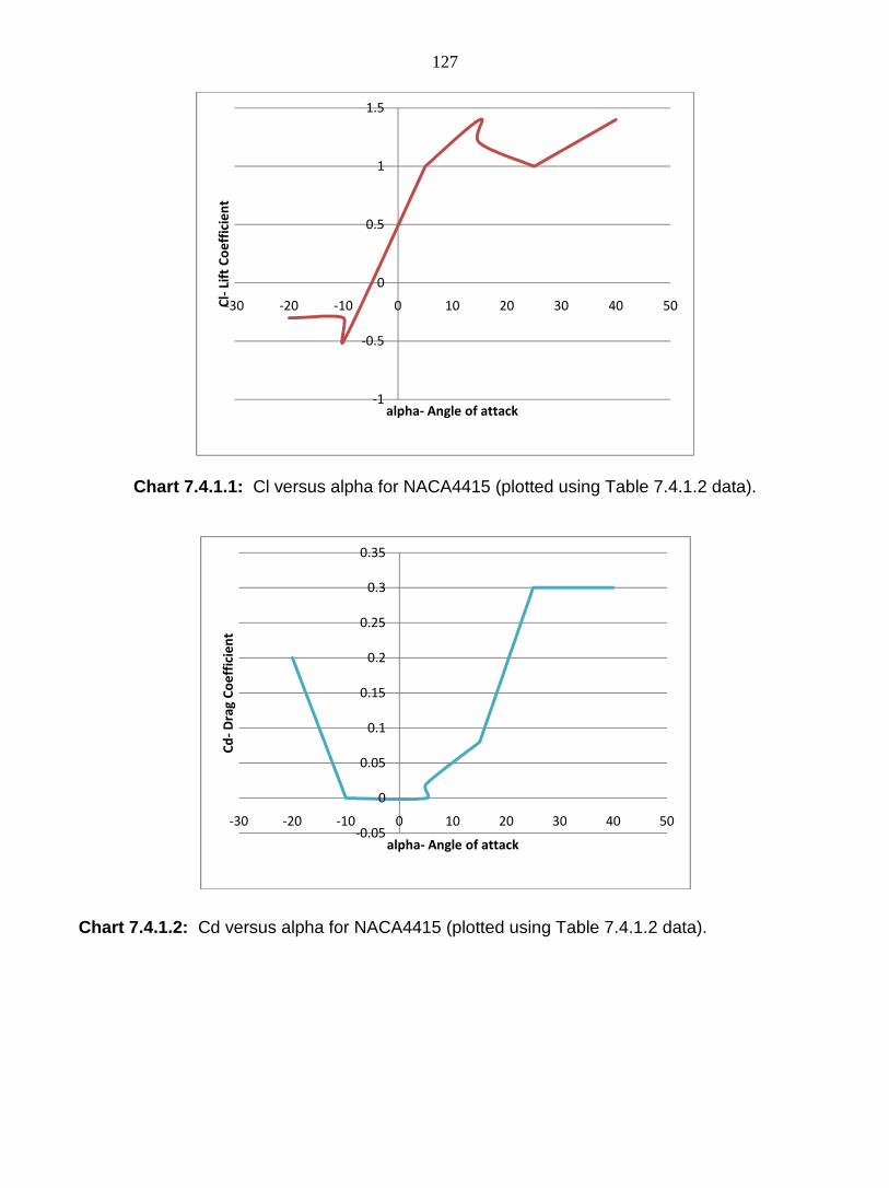
127

Chart 7.4.1.1: Cl versus alpha for NACA4415 (plotted using Table 7.4.1.2 data).

Chart 7.4.1.2: Cd versus alpha for NACA4415 (plotted using Table 7.4.1.2 data).

-1

-0.5

0

0.5

1

1.5

-30 -20 -10 0 10 20 30 40 50Cl-

Lift

Co

eff

icie

nt

alpha- Angle of attack

-0.05

0

0.05

0.1

0.15

0.2

0.25

0.3

0.35

-30 -20 -10 0 10 20 30 40 50

Cd

-D

rag

Co

eff

icie

nt


128

Chart 7.4.1.3: Cm versus alpha for NACA4415 (plotted using Table 7.4.1.2 data).

7.4.2 S809 Airfoil Profile Properties Below Table 7.4.2.1 show the S809 airfoil coordinates [33, 85] where the size of the airfoil

shape depends directly on the size of its chord.

Upper

Surface

Lower

Surface

x/c y/c x/c y/c

0.00037 0.00275 0.0014 -0.00498

0.00575 0.01166 0.00933 -0.01272

0.01626 0.02133 0.02321 -0.02162

0.03158 0.03136 0.04223 -0.03144

0.05147 0.04143 0.06579 -0.04199

0.07568 0.05132 0.09325 -0.05301

0.1039 0.06082 0.12397 -0.06408

0.1358 0.06972 0.15752 -0.07467

0.17103 0.07786 0.19362 -0.08447

0.2092 0.08505 0.23175 -0.09326

0.24987 0.09113 0.27129 -0.1006

-0.4

-0.35

-0.3

-0.25

-0.2

-0.15

-0.1

-0.05

0

0.05

-30 -20 -10 0 10 20 30 40 50

Cm

-P

itch

Mo

me

nt

Co

eff

icie

nt


0.29259

0.33689

0.38223

0.42809

0.47384

0.52005

0.56801

0.61747

0.66718

0.71606

0.76314

0.80756

0.84854

0.88537

0.91763

0.94523

0.96799

0.98528

0.99623

1

Table 7.4.2.1: By plotting these coordinates, we can obtain the geometrical shape of the

shown in Fig. 7.4.2.1

Fig. 7.4.2.1: Geometrical shape of S809 a

-0.2

0

0.2

0.4

0.6

0.8

1

1.2

0

y/c

129

0.09594 0.31188 -0.10589

0.09933 0.35328 -0.10866

0.10109 0.39541 -0.10842

0.10101 0.43832 -0.10484

0.09843 0.48234 -0.09756

0.09237 0.52837 -0.08697

0.08356 0.57663 -0.07442

0.07379 0.62649 -0.06112

0.06403 0.6771 -0.04792

0.05462 0.72752 -0.03558

0.04578 0.77668 -0.02466

0.03761 0.82348 -0.01559

0.03017 0.86677 -0.00859

0.02335 0.90545 -0.0037

0.01694 0.93852 -0.00075

0.01101 0.96509 0.00054

0.006 0.98446 0.00065

0.00245 0.99612 0.00024

0.00054 1 0

0 0 0

Coordinates of S809 airfoil profile [33, 35,

By plotting these coordinates, we can obtain the geometrical shape of the

eometrical shape of S809 airfoil (plotted using Table 7.4.2.1data)

0.2 0.4 0.6 0.8 1 1.2

x/c

0.10589

0.10866

0.10842

0.10484

0.09756

0.08697

0.07442

0.06112

0.04792

0.03558

0.02466

0.01559

0.00859

0.00075

, 85].

By plotting these coordinates, we can obtain the geometrical shape of the S809 airfoil as

Table 7.4.2.1data).

1.2

130

The S809 Wind Tunnel Profile Coefficients Cl, Cd and Cm w.r.t. the angle of attack shown in

Table 7.4.2.2. This relations were obtained at the Delft University of Technology Low Speed

Laboratory low-turbulence wind tunnel with a Reynolds number of 1,000,000 ,Somers [85, 86].

Angle of

Attack Cl Cd Cm

-1.04 0.019 0.0095 -0.0408

-0.01 0.139 0.0094 -0.0435

1.02 0.258 0.0096 -0.0462

2.05 0.378 0.0099 -0.0487

3.07 0.497 0.01 -0.0514

4.1 0.617 0.01 -0.0538

5.13 0.736 0.0097 -0.056

6.16 0.851 0.0095 -0.0571

7.18 0.913 0.0127 -0.0506

8.2 0.952 0.0169 -0.0439

9.21 0.973 0.0247 -0.0374

10.2 0.952 0.0375 -0.0397

11.21 0.947 0.0725 -0.0345

12.23 1.007 0.0636 -0.042

13.22 1.031 0.0703 -0.042

14.23 1.055 0.0828 -0.0419

15.23 1.062 0.1081 -0.0418

16.22 1.043 0.1425 -0.0452

17.21 0.969 0.1853 -0.0458

18.19 0.938 0.1853 -0.0544

19.18 0.929 0.1853 -0.0658

20.16 0.923 0.1853 -0.0783

Table 7.4.2.2: Cl, Cd and Cm w.r.t. angle of attack for S809 airfoil [33, 35, 85].

Using the linear interpolation and extrapolation techniques, we can extend the values of

coefficients Cl, Cd and Cm w.r.t. alpha of Table 7.4.2.2 to include all the required coefficients

for other required angle of attack values as shown.

131

Linear interpolation

(7.4.2.1) ` Linear extrapolation

(7.4.2.2)

Plotting the corresponding Cl w.r.t alpha, Cd w.r.t. alpha and Cm w.r.t. alpha, for the S809,

we obtain chart 7.4.2.1, chart 7.4.2.2 and chart 7.4.2.3 respectively.

Chart 7.4.2.1: Cl versus alpha for S809 (plotted using Table 7.4.2.2 data).

0

0.2

0.4

0.6

0.8

1

1.2

-5 0 5 10 15 20 25

Cl-

Lift

Co

eff

icie

nt


132

Chart 7.4.2.2: Cd versus alpha for S809 (plotted using Table 7.4.2.2 data).

Chart 7.4.2.3: Cm versus alpha for S809 (plotted using Table 7.4.2.2 data).

0.005

0.025

0.045

0.065

0.085

0.105

0.125

0.145

0.165

0.185

-5 0 5 10 15 20 25

Cd

-D

rag

Co

eff

icie

nt


-0.08

-0.07

-0.06

-0.05

-0.04

-0.03

-5 0 5 10 15 20 25

Cm

-P

itch

Mo

me

nt

Co

eff

icie

nt


133

By interpolating or by looking precisely at these charts we can easily obtain the associated

values of Cl, Cd and Cm at each station of the our blade by only knowing the angle of attack.

And by knowing the values of Cl, Cd and Cm, and some other necessary blade properties, I

will able obtain the aerodynamic loading as Fx, Fy, Fz, Mx, My and Mz.

The angle of attack definition and its relation to other important angles will be discussed in

next section because understanding this is so important for the blade aerodynamic loading

calculation.

7.5 Blade Different Airfoil Geometrical Properties

Considering the present blade of 14m length, as shown in Fig 7.5.1, where the blade is

divided into 15 stations. Each of two consecutive stations is separated by 1m.

Fig. 7.5.1: Blade different airfoil profiles.

The blade profile at each of these stations is shown in Table 7.5.1, where the NACA4415

airfoil profile was considered for all stations that linearly increasing in cross section from station

134

1 to station 2 and linearly decreasing in cross section from station 2 to station15 (at tip of the

blade).

Station(m)

Chord(m) Thickness(m)

Profile

Airfoil station Twist angle

x-location(m) (degree)

1 0 0.542 0.11382 14 NACA4415

2 1 1.467035 0.30807735 13 NACA4415

3 2 1.401105 0.29423205 12 NACA4415

4 3 1.35518 0.2845878 11 NACA4415

5 4 1.269245 0.26654145 10 NACA4415

6 5 1.2033 0.252693 9 NACA4415

7 6 1.137385 0.23885085 8 NACA4415

8 7 1.071455 0.22500555 7 NACA4415

9 8 1.005525 0.21116025 6 NACA4415

10 9 0.939595 0.19731495 5 NACA4415

11 10 0.873665 0.18346965 4 NACA4415

12 11 0.807735 0.16962435 3 NACA4415

13 12 0.741805 0.15577905 2 NACA4415

14 13 0.675875 0.14193375 1 NACA4415

15 14 0.675875 0.14193375 0 NACA4415

Table 7.5.1: Blade stations airfoil profile properties.

By knowing or by computing the angle of attack ( ) at each station by using , as

was discussed in section 7.3, then we can select the associated Cl, Cd and Cm coefficients at

each station of the blade by using the charts 7.4.1.1, 7.4.1.2 and 7.4.1.3. Some authors

assume that change in relation with the blade azimuth angle as shown in Fig. 7.5.2 [87]

where inboard alpha is higher than the outboard alpha and alpha incrementaly decreases from

azimuth angle zero to azimuth angle 180 and then incremently increases from azimuth angle

180 degrees to azimuth angle 360 degrees to go back to the same value that it was at zero

degree .

α α βφ −=

α

135

Fig. 7.5.2: Angle of attack versus Azimuth angle [87]. Other authors might model the wind gust as a sinusoidal change of the angle of attack ( )

where it changes as a function of time, for example, = 15 + 10 sin 6t as was given by

references [28, 88] which is in agreement of the present author’s assumption.

Consider the blade rotational speed 8|, wind flow angle , blade relative speed >;9| as given in Eqns 7.5.1, 7.5.2 and 7.5.3 respectively.

8| Ω U| (7.5.1)

atan WU/8|Z (7.5.2)

>;9| 5 G 8|j.s (7.5.3)

where , Ω and U are defined as given in Table 7.5.2.

Air density (rho) kg/m3 1.25

rpm 43

Angular speed (omega) = 2 rpm/60 4.5029

Mean free stream wind speed U- m/s 25

Table 7.5.2: Wind properties.

α

α

ρ

Ω π

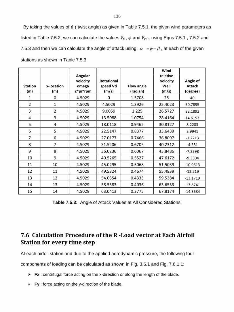
136

By taking the values of ( twist angle) as given in Table 7.5.1, the given wind parameters as

listed in Table 7.5.2, we can calculate the values 8|, and >;9| using Eqns 7.5.1 , 7.5.2 and

7.5.3 and then we can calculate the angle of attack using, , at each of the given

stations as shown in Table 7.5.3.

Station

(m)

Angular

velocity

omega

2*pi*rpm

Rotational

speed Vti

(m/s)

Wind

relative

velocity

Vreli

(m/s)

x-location

(m)

Flow angle

(radian)

Angle of

Attack

(degree)

1 0 4.5029 0 1.5708 25 40

2 1 4.5029 4.5029 1.3926 25.4023 30.7895

3 2 4.5029 9.0059 1.225 26.5727 22.1892

4 3 4.5029 13.5088 1.0754 28.4164 14.6153

5 4 4.5029 18.0118 0.9465 30.8127 8.2283

6 5 4.5029 22.5147 0.8377 33.6439 2.9941

7 6 4.5029 27.0177 0.7466 36.8097 -1.2213

8 7 4.5029 31.5206 0.6705 40.2312 -4.581

9 8 4.5029 36.0236 0.6067 43.8486 -7.2398

10 9 4.5029 40.5265 0.5527 47.6172 -9.3304

11 10 4.5029 45.0295 0.5068 51.5039 -10.9613

12 11 4.5029 49.5324 0.4674 55.4839 -12.219

13 12 4.5029 54.0354 0.4333 59.5384 -13.1719

14 13 4.5029 58.5383 0.4036 63.6533 -13.8741

15 14 4.5029 63.0413 0.3775 67.8174 -14.3684

Table 7.5.3: Angle of Attack Values at All Considered Stations.

7.6 Calculation Procedure of the R -Load vector at Each Airfoil

Station for every time step At each airfoil station and due to the applied aerodynamic pressure, the following four

components of loading can be calculated as shown in Fig. 3.6.1 and Fig. 7.6.1.1:

Fx : centrifugal force acting on the x-direction or along the length of the blade.

Fy : force acting on the y-direction of the blade.

α βφ −=

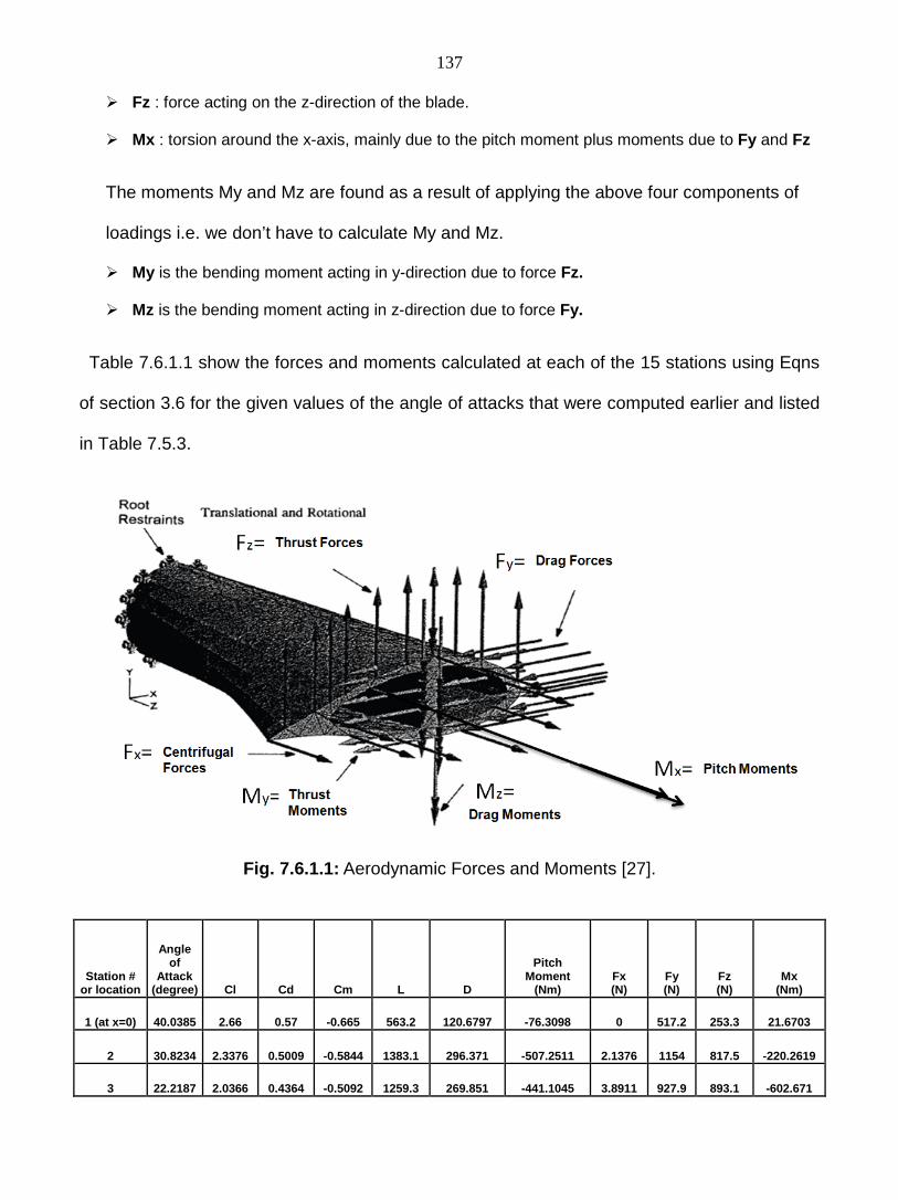
137

Fz : force acting on the z-direction of the blade.

Mx : torsion around the x-axis, mainly due to the pitch moment plus moments due to Fy and Fz

The moments My and Mz are found as a result of applying the above four components of

loadings i.e. we don’t have to calculate My and Mz.

My is the bending moment acting in y-direction due to force Fz.

Mz is the bending moment acting in z-direction due to force Fy.

Table 7.6.1.1 show the forces and moments calculated at each of the 15 stations using Eqns

of section 3.6 for the given values of the angle of attacks that were computed earlier and listed

in Table 7.5.3.

Fig. 7.6.1.1: Aerodynamic Forces and Moments [27].

Station # or location

Angle of

Attack (degree) Cl Cd Cm L D

Pitch Moment

(Nm) Fx (N)

Fy (N)

Fz (N)

Mx (Nm)

1 (at x=0) 40.0385 2.66 0.57 -0.665 563.2 120.6797 -76.3098 0 517.2 253.3 21.6703

2 30.8234 2.3376 0.5009 -0.5844 1383.1 296.371 -507.2511 2.1376 1154 817.5 -220.2619

3 22.2187 2.0366 0.4364 -0.5092 1259.3 269.851 -441.1045 3.8911 927.9 893.1 -602.671

138

4 14.6409 1.7715 0.3796 -0.4429 1193.7 255.7982 -398.4579 5.2877 760.3 955.2 -109.8173

5 8.2507 1.548 0.3317 -0.387 1165.9 249.8318 -369.9474 6.3544 634.2 1009.7 -84.6115

6 3.0139 1.3732 0.3 -0.3332 1169 255.3842 -341.3525 7.1184 537.1 1069.2 -58.5652

7 -1.2037 1.2608 0.3 -0.263 1214.4 288.9575 -288.0977 7.6067 455.3 1162.3 -0.9592

8 -4.565 1.1712 0.3 -0.207 1269.4 325.1634 -240.3757 7.8466 384.2 1252.8 48.3634

9 -7.2252 1.1003 0.3 -0.1627 1329.5 362.4979 -197.6454 7.8651 321.9 1339.9 89.7716

10 -9.3169 1.0445 0.3 -0.1278 1390.8 399.4572 -159.9229 7.6892 267.3 1422.1 123.0573

11 -10.949 1.001 0.3 -0.1006 1450 434.5373 -127.3623 7.3462 220 1497.6 147.8931

12 -12.207 1.0244 0.2732 -0.0927 1592 424.5552 -116.3497 6.8631 253.5 1628 159.6402

13 -13.16 1.0434 0.2522 -0.087 1714.9 414.5148 -106.0269 6.267 283.3 1741.4 164.2314

14 -13.863 1.0575 0.2368 -0.0828 1809.9 405.2416 -95.7305 5.585 306.3 1829.3 161.8792

15 (at x=L) -14.358 1.0674 0.2259 -0.0798 1871.4 39 6.0582 -85.3276 4.8443 321.7 1885.6 153.0529

Table 7.6.1.1: Aerodynamic forces and moments at different stations in and about x,y and z

directions. This will enable us to calculate all the interpolated force functions that represent all the station

forces , and and to calculate all the interpolated moment function of all the

station moments as a function of x ( the coordinate along the blade length) using the

MATLAB code of the present research.

The aerodynamic load vector tR ( i.e. the right side of the dynamic equations of motion) can

be computed using the following Eqn 7.6.1.

)(xFx )(xFy )(xFz

)(xM x

139

=

==

∫

∫

∫

∫

∫

∫

∫

∫

∫

∫

∫

∫

∫

∫

∫

∫

∫

∫

L

x

L

x

L

z

L

z

L

y

L

y

L

z

L

z

L

y

L

y

L

x

L

x

L

mx

L

mz

L

my

L

mz

L

my

L

mx

t

dxxxM

dxxxM

dxxxM

dxxxM

dxxxM

dxxxM

dxxxF

dxxxF

dxxxF

dxxxF

dxxxF

dxxxF

dxxxM

dxxxM

dxxxM

dxxxF

dxxxF

dxxxF

RtimeloadR

0

2

0

1

0

2

0

1

0

2

0

1

0

2

0

1

0

2

0

1

0

2

0

1

0

0

0

0

0

0

)()(

)()(

)()(

)()(

)()(

)()(

)()(

)()(

)()(

)()(

)()(

)()(

)()(

)()(

)()(

)()(

)()(

)()(

)(_

φ

φ

φ

φ

φ

φ

φ

φ

φ

φ

φ

φ

φ

φ

φ

φ

φ

φ

(7.6.1) Specifying , for example, that m= 1 to M=2, implies that 2

1 )/()( Lxx =φ and 32 )/()( Lxx =φ

since the given polynomial expansion is 1)/()( += mm Lxxφ as was discussed in section 3.5.

It should be noted that all the above steps of the calculation of the load vector tR have to be

repeated for each of the given time steps since tR is a function of the angle of attack ( which is

function of the given time steps) at the given blade stations.

140

Chapter 8

Implementation and Numerical Results

8.1 Introduction

Consider that the present blade for both examples of the next two sections 8.2.1 and 8.2.2

share the following assumptions:

The blade has a 14 m length and a Young’s modulus of 17 GPa.

The blade is clamped at one end (cantilever) and submitted to non-uniformly distributed

aerodynamic forces (described above), to centrifugal forces and gravitational forces moving

with an angular velocity Ω of 4.5029 rad/s.

Wind turbine rotor is in upwind configuration.

The blade airfoil section is of NACA4415 type and is wise-piece variable along the

radius.

The nacelle is adjustable with a yaw angle that varies so as to always align the

wind velocity normal to the rotation plan of the blade, so that the yaw error can be

neglected.

The connection between the blade and the hub is rigid.

The deformation is large.

The analysis of the blade’s response concerns the study of the behavior of the blade

submitted to a gust of wind of 25 m/s speed during 3 s. The direction of the gust is

considered parallel to the axis of the hub (rotor).

The wind’s attack angle to the blade varies as a function of time, according to α = 15 + 10

sin 6t . This assumption means that the variation of the gust excitation is modeled by the

variation of the attack angle.

141

It should be noted that the blade share the same geometry of NACA4415 as the blade for the

linear case example ( section 8.2.1 ) that was studied by Younsi et al. [28].

But for the nonlinear example case ( section 8.2.2 ), the blade is different from that given by

Younsi et al. [28] by the following differences:

The nonlinear blade example has a pretwisted geometry as mentioned above.

The nonlinear blade example has a lower material density.

The nonlinear blade example considers the large deformation case while Younsi et

al. [28] considered only the small deformation case.

8.2 Numerical Application and Results

8.2.1 Linear Small Deformation Case Example

Consider an untwisted 14 m length blade of a Young’s modulus of 17 GPa and a material

density of 600 Kg/m3, as listed in the below Table 8.2.1.1, that behave in a linear small

deformation.

Table 8.2.1.1: Blade properties for the linear example.

It should be noted again that we are considering the same problem that was solved by Younsi

et al. [28] so that we can compare our solution by their solution. The application concerns the

study of the behavior of the blade submitted to a gust of wind of 25 m/s speed during 3

seconds. Fig. 8.2.1.1 shows the main dimensions of the blade, the line of the centers of

gravity as well as the line of aerodynamic centers.

142

Fig. 8.2.1.1: Blade geometry and neutral axis line as given by Younsi et al. [28] The aerodynamic forces Fx, Fy and Fz and the aerodynamic moments Mx, My and Mz were

calculated at all the given 15 stations (or nodes) using the formulas listed in section 3.6 and

section 7.6 and input to the Ls-Dyna model using Hypermesh as shown in Fig. 8.2.1.2.

Fig. 8.2.1.2: Forces and Moments at all the given 15 Stations.

While for the MATLAB code (present research code), all these aerodynamic forces and

moments were interpolated to have them as function of x ( the coordinate along the length of

the blade) and this process have to be repeated for each of the given time steps in order to

obtain the R-load vector per Eqn 7.6.1 (as was explained in section 7.6). By having all the

derived linear mass, dynamic and stiffness matrices (that derived in section 5.2) and the

143

calculated R-load vector at each time step, the author was able to solve the dynamic equation

of motion( Eqn 6.1.1a) using the MATLAB code and the linear Newmark iteration scheme (that

was explained in section 6.4) for the vibration response at all the given blade stations. Below

in Fig. 8.2.1.2, the displacements and rotations at the blade’s tip are shown:

Fig. 8.2.1.2: Blade tip linear displacements and rotations. (a) Displacement in x-direction; (b) Displacement in y-direction;

(c) Displacement in z-direction; (d) Rotation about y-direction; (e) Rotation about z-direction; and (f) Rotation about x-direction

Fig. 8.2.1.3 shows a two-plot comparison of the blade’s tip displacement in the vertical

flapwise direction between the present work and that of Younsi et al. [28] for the same blade

problem. In Fig. 8.2.1.3 (a), the peak and stabilized displacements are 1.75m and 1.021 m

144

respectively while the peak and stabilized displacements values in Fig. 8.2.1.3 (b) are 1.68 m

and 0.92 m. We observe that both plots have the same kind of trend but the current study has

lower peak and steady state displacements. Current work not only shows an agreement with

the hypothesis of the linearity of the solution introduced by Younsi et al. but also has lower

displacement values. This is due to the fact of the inclusion of all the loadings and their

couplings and the blade’s cross-sectional warping. Note that the vertical direction is along the

z-axis in this work while it is along the y-axis in the work of Younsi et al. [28] .

Fig. 8.2.1.3: Comparison of (a) Younsi et el. published work [28].

(b) present work.

8.2.2 Non-linear Large Deformation Case Example

Consider a pretwisted 14 m length blade of a Young’s modulus of 17 GPa and a material

density of 500 Kg/m3, as listed in the below Table 8.2.2.1, that behave in a nonlinear large

deformation.

145

Table 8.2.2.1: Blade properties for the non-linear example.

The present blade is modeled as a combination of 14 beams (each of 1m length) separated

by 15 main nodes or stations. The pre-twist angles for these 15 stations as going from the hub

to the tip of the blade are respectively equal to 14,13,12,11,10,9,8,7,6,5,4,3,2,1 and 0.

It should be noted that the pretwist of the present blade change the values of the geometrical

properties at each of the given blade stations from those calculated by Younsi et al. [28].

The aerodynamic forces and moments were calculated and then interpolated as a function of

the lengthwise x of the blade using the same method of the linear example of previous section

8.2.1. By having all the linear mass, dynamic and stiffness matrices (that derived in section

5.2) and the nonlinear stiffness matrices (that derived in section 5.3) and the calculated R-load

vector at each time step, the author was able to solve the nonlinear dynamic equation of

motion (6.1.1b) using the MATLAB code and the nonlinear Newmark iteration scheme (that

was explained in section 6.6) for the vibration response at all the given blade stations. The

displacements and rotations were computed at all the 15 blade stations. (where node# 15 as

mentioned earlier is the location of the blade’s tip).

The obtained solution was compared by the the same blade’s response solution using the ls-

Dyna code that was built using the same blade’s material and geometrical properties with the

same applied loading across the blade that considered for the Matlab code.

Fig. 8.2.2.1, Fig. 8.2.2.2 and Fig. 8.2.2.3 show the displacements at the blade’s in x, y and z-

directions respectively, using the current study Matlab code and the ls-dyna code. And Fig.

8.2.2.4, Fig. 8.2.2.5 and Fig. 8.2.2.6 show the rotational displacement at the blade’s tip about

the x, y and z directions respectively, using the Matlab code and the ls-Dyna code.

146

Fig. 8.2.2.1: Nonlinear plots comparison for tip displacement in x-direction.

(a) Displacement in x-direction using present work; (b) Displacement in x-direction using Ls-Dyna.

Fig. 8.2.2.2: Nonlinear plots comparison for tip displacement in y-direction.

(a) Displacement in y-direction using present work; (b) Displacement in y-direction using Ls-Dyna.

147

Fig. 8.2.2.3: Nonlinear plots comparison for tip displacement in z-direction.

(a) Displacement in z-direction using present work; (b) Displacement in z-direction using Ls-Dyna.

Fig. 8.2.2.4: Nonlinear plots comparison for tip rot. displ. about x-direction.

(a) Rotational displacement about x-direction using present work; (b) Rotational displacement about x-direction using Ls-Dyna.

148

Fig. 8.2.2.5: Nonlinear plots comparison for tip rot. displ. about y-direction.

(a) Rotational displacement about y-direction using present work; (b) Rotational displacement about y-direction using Ls-Dyna.

Fig. 8.2.2.6: Nonlinear plots comparison for tip rot. displ. about z-direction.

(a) Rotational displacement about z-direction using present work; (b) Rotational displacement about z-direction using Ls-Dyna.

149

Chapter 9

Conclusion and Related Future Work

9.1 Conclusion For the linear example case, the present study plot of the displacement in the vertical

direction at the blade’s tip agrees agrees as far as trend with the plot of the same displacement

that were given by Younsi et al. study [28] even that both plots has different peak values. The

advantage of the present study method on Younsi et al. study [28] is the accuracy of the

obtained displacements and rotations solution due to the inclusion of the cross-sectional

warping of the blade and the consideration of all the aerodynamic loads and all the possible

load couplings that acting on the blade. The other advantage is the capability of the present

research method of solving the displacements and rotations for any pretwisted blade while

Younsi et al. [28] study was limited to the untwisted blade case. It is observed that there is a

delay of about 3 seconds before the rapid increase in deflection in Fig. 8.2.1.3 (a) compared to

Fig. 8.2.1.3 (b). This delay is due to the additional aerodynamic interactions that caused by

the CFD code by which Younsi et al. study [28] performed the aerodynamic load prediction.

For the nonlinear example case, the nonlinear large deformation mathematical model for the

present 14 m pretwisted wind turbine blade lead to have a set of higher order terms that

contribute to the formation of two additional non-linear stiffness matrices.

We observe in Fig. 8.2.2.3 (a) and Fig. 8.2.2.3 (b) that the steady state blade’s tip nonlinear

displacement in the vertical z-direction for both codes (the present study Matlab code and the

Ls-Dyna code), is about 4m which is about 28% of the 14 m (length of the blade). This is in

agreement with the hypothesis introduced by Younsi et al. [28] that displacement is considered

to be nonlinear if exceeds 10% of the length of the blade.

150

We also observe that even we have a similar trend of all the displacement and rotation plots

for both codes solutions as shown in Fig. 8.2.2.1 to Fig. 8.2.2.6, the peak and/or the steady

state values are vary in many of these plots. For example, in Fig. 8.2.2.3 (a), the peak

displacement using the present study Matlab code is 6.2 m while in Fig. 8.2.2.3 (b), the peak

displacement using the ls-dyna is 7.3 m. This variation is normal and it is due to the inclusion

of the following additional factors in the author’s present research mathematical model (Matlab

code) that are not included in the Ls-Dyna code:

The additional aerodynamic load couplings.

The two additional nonlinear stiffness matrices of the dynamic equations of motion due to

the nonlinear large deformation assumption.

The following are number of contributions for the present research:

A new simple method that based on the airfoil wind tunnel aerodynamic parameters

collected data (not based on CFD or the Bezier interpolation scheme) to calculate the R

load vector.

The mathematical formulation of this present research is capable of generating the

displacements, velocities and acceleration at any point on the blade for small or large

displacement for any duration of the aerodynamic loadings ( for example, it can run for

days) while Ls-dyna and similar current commercial softwares has a limited input data

storage and the aerodynamic load data has to be entered manually.

The present research MATLAB code is the only current code the is able to update the

angle of attack by the value of the twisting rotation phi about the x-axis ( along the

length of the blade).

calculation of the geometrical properties of any given blade airfoil profiles using a new

created macro to be used within Hypermesh.

151

The inclusion of warping and all the possible aerodynamic loadings and their couplings

beside the rotary inertia, shear deflection.

No need to send my files to the Grid or to Gigastar in order to solve as happening in

case of current dynamic codes.

9.2 Related Future Work My plan is to extend the present wind turbine blade research to include the following

improvement to my present research MATLAB code:

Add the capability to solve blades with plastic and composite materials.

Improve the code to be able to compute the natural frequencies and plot the mode

shapes for any given blade inputs.

To be able to identify the rpm(s) of the blade that the blade designer need to avoid in

order to avoid any possible excitation of the blade natural frequency.

152

APPENDIX A: DERIVATION OF THE DIFFERENT STRAIN ENERGIES

A. 1. Axial-Torsional Strain Energy Including Warping Effect Two common assumptions are made for the coupled extension-torsion problem: first, that

deformation parallel to the cross-sections is negligible, and second, that axial deformation

consists of bulk displacement u and cross sectional warping.

Airfoil warping in wind turbine blade application is assumed to be constant throughout the

cross section (or station) and vary in value between the different stations i.e. W, $, %Z WZ

only.

To derive the axial-torsional strain energy for the pre-twisted Timoshenko beam of Fig. 3, we

have to start with the Green’s strain-displacement relation in order to express the strain energy

in terms of large displacement fields [22]:

This implies that the resulting strain components are:

+ [ + 22θr ] where

but = + + where = , and 21

21

2 zyr +=

where , as stated earlier, is the angle of elastic rotation additional to the pre-twist angle .

This implies that:

= + +

Substituting for in xzxyxx andεεε ,

=xxε + + + [ 2)(x

u

∂∂

+ 22θr ]

( )jij

i

i

jij x

u

x

u

x

u

x

u

∂

∂

∂

∂+

∂

∂+

∂

∂= ααε

x

uxx ∂

∂=ε

2

1)(

x

u

∂

∂2

x

u

∂

∂xxε

x∂

∂ψθ ψ

θ

x∂

∂xxε

x

u

∂∂

x∂

∂=

φθ

φ β

x

u

∂

∂

x

u

∂∂

x∂

∂ψθ ψ

θ

x∂

∂

x

u

∂

∂

x

u

∂∂

x∂

∂ψθ ψ

θ

x∂

∂

2

1

153

It should be noted that keeping the following high order terms:

[ 2)(x

u

∂∂

+ 22θr ]

in the below derivation is an important contribution of the present work.

Expanding, implies:

=xxε + + + 2)(x

u

∂∂

+ 2)(x∂

∂ψθ

+ + 2)( ψ

θx∂

∂ +

+ + 22θr

Since warping is a function of x only implies: 0=∂∂

=∂∂

zy

ψψ, which implies,

[ 1+ ]1z− = θ ][ 1z−

[ 1+ ]1y+ = ][ 1yθ

2

1 2θ [ ] = 0, 2

1 2θ [ ] = 0 and2

1 2θ [ ] =0

The result is the axial-torsional strain energy which is in agreement with [22, 36] :

2

xxε + 2 G ( 2xyε +

2xzε ) 2φ ′′ (A.1)

A. 2. Bending-Bending-Shear Coupling Strain Energy The strain energy due the blade’s bending about the y and z directions and their couplings

2

1

x

u

∂∂

x∂

∂ψθ ψ

θ

x∂

∂

2

1

2

1

x

u

∂∂

x∂

∂ψθ

2

1

x

u

∂∂

ψθx∂

∂

x∂

∂ψθ ψ

θ

x∂

∂

2

1

=xyε2

1θ (

y∂

∂ψ

x

u

∂

∂)

2

1

=xzε2

1θ (

z∂

∂ψ

x

u

∂

∂)

2

1

=yyεy∂

∂ψ2 =yzε

y∂

∂ψ

z∂

∂ψ=zzε

z∂

∂ψ2

torsionalaxialU − EdydzA

L

2

1

0∫∫∫= dx p

L

EI2

1

0∫+ dx

154

including the effect of deflection due to transverse shear in two planes i.e. the case of

Timoshenko beam [18, 21, 40] is:

= ( 21θ ′ + 2 + 2

2θ ′ ) + + dx

(A.2) where,

W ′ Z : means derivative w.r.t. x

k : is the shear correction factor

kGA: is the shear rigidity

: are the second moment of area of the cross-section through the centroid about the

and axes respectively as shown in Fig. 3.2.1.

: is the product moment of area of the cross-section about the and axes as

shown in Fig. 3.2.1.

A. 3. Bending-Torsional Coupling Strain Energy

The blade structure will undergo torsional deformation as it flexes because of its asymmetrical

airfoil cross-section where the shear centres axis and the centroid centres axis are not

coincident [21, 39] :

=−torsionbendingU PL

∫02

1 [ - 2 'v + )/( AI p ] dx + P

L

∫02

1 [ - 2 'w + )/( AI p ] dx

+ dxAwEL

4

0

'4

1

2

1∫ + dxwIE p

L22

0

''2

1

2

1φ∫ + + (A.3)

where P is the axial force.

shearbendingU − EL

∫02

1yyI yzI '1θ '2θ zzI )'(( 1θ−wkGA 2 )'( 2θ−v 2

,yyI zzI 1y

1y 1z 1z

yzI 1y 1y 1z 1z

2v′ αy 'φ 2φ ′ 2w′ αz 'φ 2φ ′

[∫L

0 1K '1θ φ′ 2K '2θ φ′ ] dx

155

Appendix B: DERIVATION OF THE DIFFERENT KINETIC ENERGIES

B. 1. Kinetic Energy due to Axial-Torsional Effect To express the axial-torsional kinetic energy in terms of the displacement field, the velocity

vector of each point in the beam is given by:

zyx ezyezyeu ˆ)sincos(ˆ)cossin(ˆ)( φφφφφφψθ −+−−++=••••

[ ]φφφφψθ eereu rx ˆ)(cosˆ)(sinˆ)( +−++=•••

(B.1)

where x∂

∂=

φθ

and dot means derivative w.r.t. time.

The cartesian unit vectors are transformed to cylindrical unit vectors ,

where and .

The kinetic energy due to axial torsional coupling effects is given by

(B. 1.1)

Substituting of from Eq. (B. 1) into Eq. (B.1.1) results in the following equation [22] :

where, 21

21

2 zyr += , which implies,

=1T +•

)(2

xAu )(xA + 2)(x∂

∂•

φ)(xA + ]dxxI p

2

)(•

φ (B.1.2)

•

R

=•

R =•

u +•

xeu ˆ)( +•

yev ˆ)( zew ˆ)(•

( ,ˆye )ˆze ( ,ˆre )φe

=re +yeyr

ˆ(1

)ˆzez =φe +− yezr

ˆ(1

)ˆzey

dVRTV

2

1 2

1 •

∫∫∫= ρ

•

R

[)(2

11 xT

V

ρ∫∫∫= +• 2

u•

u2 +•

ψθ +•

22

ψθ ] dVr2

2•

φ

[)(2

1

0

xL

ρ∫•

u2 )(

•

∂∂

x

φψ

2ψ

156

B. 2. Kinetic Energy due to Bending-Torsion including Centrifugal

Effect The kinetic energy due to bending-bending-torsional coupling including centrifugal effect by

keeping the important higher order terms up to 4th order is [18, 21, 24, 89] :

=2T 422222

2222222

22

0

)(4

1)()()()(

2

1φφθφθρ xAyxAzxAyxAzx

L

Ω+Ω−Ω−Ω∫ 22 )( uxAΩ+

•

Ω+ 222 )(2 θφxAy 2

2 )(2•

Ω− θφxAz +Ω+•

232 )( θφxAz )(2 xAz 2

2

•

θ 22

22 )(•

− θφxAz•

Ω+ φθ22 )(2 xAy

)(2 2 xAzΩ+••

Ω− φφθφθ 22

22 )(xAy 2zΩ− )(xA +

•

φφθ 22

••

φθφθ 222 )(2 xAy

••

− φθφθ 222 )(2 xAz )(2 xAy+

22

2

)(••

+ φφ xAz dxxAy2

22

2 )(•

+ φθ [ ]dxywzvxmL

22

0

)()()(2

1 ••••

++++ ∫ φφ αα zz

L

Ix)(2

1

0

ρ∫+

yyIx)(ρ+ dx [ 2

0

2

)''()(2

φαzvxmL

+Ω

− ∫ ++ '(w 2)'φαy ]xdx (B.2)

where Ω and Ω is the rotational speed and the angular velocity of the blade respectively.

B. 3. Kinetic Energy due to Rotary Inertia Effect The kinetic energy due to rotary inertia effect as given by Carnegie [18] is:

3T

(B.3)

22 )(

••

′+ φθ αz 21 )( φθ αy −′+

••

[g

zzxI zzL 2

2

0

))((

2

1•• ′+′+

= ∫φφθρ αα ] dx

g

yyxI yy2

1 ))((•• ′+′+

+φφθρ αα

157

APPENDIX C: DERIVATION OF m

Total

q

U

∂∂

Considering the total strain energy Eq. (2) shown in section 2.1, implies:

Substituting for,

, and ,

implies,

+ + + ( + ( ) + +

( ) + + +

[ 1+ + +

]1z−

[ 1+ + +

]1y+

Expanding and substituting the associated values of D’s that listed in TABLE A, results in:

+ + + (

+ + + +

+ + ( +

+ + +

dydzdxa

Gdydzdxa

Gdydzdxa

Ea

U

m

xzxz

A

L

m

xyxy

A

L

m

xxxx

A

L

m

Total

∂∂

+∂

∂+

∂∂

=∂

∂∫∫∫∫∫∫∫∫∫

εε

εε

εε

000

44

=∂∂

m

xx

a

ε+mxφ(

x

u

∂∂

+mxφx∂

∂ψθ +mxφ ψ

θ

x∂

∂)mxφ 0

2

1=

∂∂

=∂

∂mx

m

xy

yaφ

ψθ

ε0

2

1=

∂∂

=∂∂

mxm

xz

zaφ

ψθ

ε

∫∫∫=∂

∂

A

L

m

Total Ea

U

0

[x

u

∂∂

x∂

∂ψθ ψ

θ

x∂

∂

2

1)

x

u

∂∂ 2

2

1

x∂

∂ψθ 2

x

u

∂∂

x∂

∂ψθ

2

1

ψθx∂

∂ 2

x∂

∂ψθ ψ

θ

x∂

∂

x

u

∂∂

ψθ

x∂

∂

2

12r θ 2 ] +mxφ(

x

u

∂∂

+mxφx∂

∂ψθ +mxφ ψ

θ

x∂

∂

)mxφ dydzdx ∫∫∫+A

L

G0

42

1θ (

y∂

∂ψ(

x

u

∂∂

x∂

∂ψθ ψ

θ

x∂

∂) ) dydzdx0

∫∫∫+A

L

G0

42

1θ (

z∂

∂ψ(

x

u

∂∂

x∂

∂ψθ ψ

θ

x∂

∂) ) dydzdx0

=∂

∂

m

Total

a

UE [ ∫

L

0 x

u

∂∂

mxφ )(xA dx ∫L

0mxθφ )(5 xD dx ∫

L

0mxx

φθ

∂∂

)(1 xD dx2

1∫L

0

)x

u

∂

∂ 2mxφ

)(xA dx2

1∫L

0mxφθ 2 )(6 xD dx ∫

L

0 x

u

∂∂

mxθφ )(5 xD dx ∫L

02

1mxx

φθ 2)(

∂∂

)(2 xD dx ∫L

0mxx

φθ

θ∂∂

)(9 xD dx ∫L

0mxxx

uφ

θ∂∂

∂∂

)(1 xD dx2

1∫L

0

θ 2mxφ )(xI p dx + ∫

L

0

)x

u

∂∂ 2

mxφ )(xA dx ∫L

0 x

u

∂∂


0mxxx

uφ

θ∂∂

∂∂

)(1 xD dx2

1∫L

0

3)(x

u

∂∂

mxφ )(xA dx2

1∫L

0 x

u

∂∂

mxφθ 2 )(6 xD dx

158

+ ( +

+ + (

+ + + +

+ ( + +

+ + + +

+ + + +

( + +

+

+ +

+

Substituting for the displacements and their derivative expressions, implies,

=∂

∂

m

Total

a

U∑

=

N

n 1

)(xA )(xnxφ dxxmx )(φ + ∑=

N

n 1

)(5 xD )(xnxφ dxxmx )(φ + ∑=

N

n 1

)(1 xD

)(xnxxφ dxxmx )(φ ∑∑==

K

k

N

n 11

)(xA )(xnxφ )(xkxφ dxxmx )(φ ∑∑==

K

k

N

n 11

)(6 xD )(xnxφ

)(xkxφ dxxmx )(φ + ∑∑==

K

k

N

n 11

)(5 xD )(xnxφ )(xkxφ dxxmx )(φ ∑∑==

K

k

N

n 11

)(2 xD

)(xnxxφ )(xkxxφ dxxmx )(φ ∑∑==

K

k

N

n 11

)(9 xD )(xnxφ )(xkxxφ dxxmx )(φ + ∑∑==

K

k

N

n 11

)(1 xD )(xnxxφ )(xkxφ dxxmx )(φ ∑∑==

K

k

N

n 11

)(xI p )(xnxφ )(xkxφ dxxmx )(φ + ∑∑==

K

k

N

n 11

∫L

0

)x

u

∂

∂ 2mxθφ )(5 xD dx ∫

L

02

1

x

u

∂∂

mxxφ

θ 2)(∂∂

)(2 xD dx ∫L

0 x

u

∂∂

mxxφ

θθ

∂∂

)(9 xD dx ∫L

0

)x

u

∂

∂

2mxx

φθ

∂∂

)(1 xD dx2

1∫L

0

θ 2

x

u

∂∂

mxφ )(xI p dx ∫L

0 x

u

∂∂



L

0

mxxφ

θθ

∂∂

)(9 xD dx2

1∫L

0

)x

u

∂

∂ 2mxθφ )(5 xD dx

2

1∫L


L

0 x

u

∂∂

mxφθ 2 )(6 xD

dx2

1∫L

0mxx

φθ

θ 2)(∂∂

)(10 xD dx ∫L

0mxx

φθ

θ∂∂2 )(22 xD dx ∫

L

0 x

u

∂∂

mxxφ

θθ

∂∂

)(9 xD dx2

1∫L

0

mxφθ 3 )(12 xD dx ∫L

0 x

u

∂∂

mxxφ

θ∂∂

)(1 xD dx ∫L

0mxx

φθ

θ∂∂

)(9 xD dx ∫L

0mxx

φθ 2)(

∂∂

)(2 xD dx

2

1∫L

0

)x

u

∂∂ 2

mxxφ

θ∂∂

)(1 xD dx2

1∫L

0mxx

φθ

θ∂∂2 )(22 xD dx ∫

L

0 x

u

∂∂

mxxφ

θθ

∂∂

)(9 xD dx2

1∫L

0

mxxφ

θ 3)(∂∂

)(3 xD dx ∫L

0mxx

φθ

θ 2)(∂∂

)(10 xD dx ∫L

0 x

u

∂∂

mxxφ

θ 2)(∂∂

)(2 xD dx2

1∫L

0mxx

φθ

θ∂∂2

)(28 xD dx ]

E ∫L

0

na E ∫L

0

nf E ∫L

0

nf 21

+ E ∫L

0

knaa21

+ E ∫L

0

kn ff E ∫L

0

knaf21

+ E ∫L

0

kn ff + E ∫L

0

kn ff E ∫L

0

knaf21

+ E ∫L

0

kn ff E

159

)(xA )(xnxφ )(xkxφ dxxmx )(φ + ∑∑==

K

k

N

n 11

)(5 xD )(xnxφ )(xkxφ dxxmx )(φ + ∑∑==

K

k

N

n 11

)(1 xD )(xnxxφ )(xkxφ dxxmx )(φ ∑∑==

LK

lk

N

n

,

1,1

)(xA )(xnxφ )(xkxφ )(xlxφ dxxmx )(φ

∑∑==

LK

lk

N

n

,

1,1

)(6 xD )(xnxφ )(xkxφ )(xlxφ dxxmx )(φ + ∑∑==

LK

lk

N

n

,

1,1

)(5 xD )(xnxφ )(xkxφ

)(xlxφ dxxmx )(φ ∑∑==

LK

lk

N

n

,

1,1

)(2 xD )(xnxxφ )(xkxxφ )(xlxφ dxxmx )(φ + ∑∑==

LK

lk

N

n

,

1,1

)(9 xD )(xnxxφ )(xkxφ )(xlxφ dxxmx )(φ + ∑∑==

LK

lk

N

n

,

1,1

)(1 xD )(xnxxφ )(xkxφ )(xlxφ dxxmx )(φ

+ ∑∑==

LK

lk

N

n

,

1,1

)(xI p )(xnxφ )(xkxφ )(xlxφ dxxmx )(φ + ∑∑==

K

k

N

n 11

)(5 xD )(xnxφ )(xkxφ

dxxmx )(φ + ∑∑==

K

k

N

n 11

)(6 xD )(xnxφ )(xkxφ dxxmx )(φ + ∑∑==

K

k

N

n 11

)(9 xD )(xnxφ )(xkxxφ

dxxmx )(φ ∑∑==

LK

lk

N

n

,

1,1

)(5 xD )(xnxφ )(xkxφ )(xlxφ dxxmx )(φ ∑∑==

LK

lk

N

n

,

1,1

)(7 xD )(xnxφ

)(xkxφ )(xlxφ dxxmx )(φ ∑∑==

LK

lk

N

n

,

1,1

)(6 xD )(xnxφ )(xkxφ )(xlxφ dxxmx )(φ ∑=

N

n 1

∑=

LK

lk

,

1,

)(10 xD )(xnxφ )(xkxxφ )(xlxxφ dxxmx )(φ + ∑∑==

LK

lk

N

n

,

1,1

)(22 xD )(xnxφ )(xkxφ )(xlxxφ dxxmx )(φ

∑∑==

LK

lk

N

n

,

1,1

)(9 xD )(xnxxφ )(xkxφ )(xlxφ dxxmx )(φ ∑∑==

LK

lk

N

n

,

1,1

)(12 xD )(xnxφ

)(xkxφ )(xlxφ dxxmx )(φ + )(1 xD )(xnxxφ )(xkxφ dxxmx )(φ + ∑∑==

K

k

N

n 11

)(9 xD )(xnxφ )(xkxxφ dxxmx )(φ + ∑∑==

K

k

N

n 11

)(2 xD )(xnxxφ )(xkxxφ dxxmx )(φ ∑∑==

LK

lk

N

n

,

1,1

∫L

0

knaa E ∫L

0

knaf E

∫L

0

knaf21

+ E ∫L

0

lkn aaa

21

+ E ∫L

0

lkn aff E ∫L

0

lkn aaf21

+ E ∫L

0

lkn aff E ∫L

0

lkn aff E ∫L

0

lkn aaf

2

1E ∫

L

0

lkn aff E ∫L

0

knaf E ∫L

0

kn ff E ∫L

0

kn ff21

+ E ∫L

0

lkn aaf21

+ E ∫L

0

lkn fff + E ∫L

0

lkn aff21

+ E

∫L

0

lkn fff E ∫L

0

lkn fff + E ∫L

0

lkn aff21

+ E ∫L

0

lkn fff E ∑=

N

n 1∑

=

K

k 1∫L

0

knaf E ∫L

0

kn ff E ∫L

0

kn ff21

+ E

160


LK

lk

N

n

,

1,1


+ ∑∑==

LK

lk

N

n

,

1,1


LK

lk

N

n

,

1,1

)(3 xD )(xnxxφ

)(xkxxφ )(xlxxφ dxxmx )(φ + ∑∑==

LK

lk

N

n

,

1,1

)(10 xD )(xnxφ )(xkxxφ )(xlxxφ dxxmx )(φ + ∑∑==

LK

lk

N

n

,

1,1

)(2 xD )(xnxxφ )(xkxxφ )(xlxφ dxxmx )(φ ∑∑==

LK

lk

N

n

,

1,1


Further substituting for the associated S integral definitions as listed in Table B, results in:

=∂

∂

m

Total

a

U

∑

=

N

n 1AmnS ∑

=

+N

n

E1

mnDS5 ∑

=

+N

n

E1

mnDS1

' ∑∑

==

K

k

N

n 11AmnkS ∑∑

==

K

k

N

n 11

mnkDS6 + ∑∑

==

K

k

N

n 11 mnkDS

5 ∑∑==

K

k

N

n 11mnkDS

2'' ∑∑

==

K

k

N

n 11mnkDS

9'

∑∑==

K

k

N

n 11mnkDS

1' ∑∑

==

K

k

N

n 11mnkI p

S + ∑∑==

K

k

N

n 11AmnkS + ∑∑

==

K

k

N

n 11mnkDS

5 +

∑∑==

K

k

N

n 11mnkDS

1'

∑∑

==

LK

lk

N

n

,

1,1AmnklS ∑∑

==

LK

lk

N

n

,

1,1mnklDS

6 + ∑∑==

LK

lk

N

n

,

1,1

mnklDS5

∑∑==

LK

lk

N

n

,

1,1mnklDS

2'' + ∑∑

==

LK

lk

N

n

,

1,1 mnklDS

9' + ∑∑

==

LK

lk

N

n

,

1,1 mnklDS

1'

∑∑==

LK

lk

N

n

,

1,1mnklI p

S + ∑∑

==

K

k

N

n 11mnkDS

5

+ ∑∑

==

K

k

N

n 11mnkDS

6 + ∑∑==

K

k

N

n 11

mnkDS9

' ∑∑==

LK

lk

N

n

,

1,1mnklDS

5 ∑∑==

LK

lk

N

n

,

1,1mnklDS

7 ∑∑==

LK

lk

N

n

,

1,1mnklDS

6

∑∑==

LK

lk

N

n

,

1,1

mnklDS10

'' + ∑∑

==

LK

lk

N

n

,

1,1 mnklDS

22' + ∑∑

==

LK

lk

N

n

,

1,1 mnklDS

9'

∫L

0

lkn aaf21

+ E ∫L

0

lkn fff E ∫L

0

lkn aff21

+ E ∫L

0

lkn fff E ∫L

0

lkn fff E

∫L

0

lkn aff21

+ E ∫L

0

lkn fff

E na nf nf 2

1+ E knaa

2

1+ E

kn ff E knaf2

1+ E kn ff + E kn ff + E

knaf2

1+ E kn ff E knaa E knaf

E knaf2

1+ E lkn aaa

2

1+ E lkn aff E

lkn aaf2

1+ E lkn aff E lkn aff E

lkn aaf2

1+ E lkn aff E knaf E kn ff E

kn ff21

+ E lkn aaf21

+ E lkn fff + E lkn aff

21

+ E lkn fff E lkn fff E lkn aff21

+ E

161

∑∑==

LK

lk

N

n

,

1,1 mnklDS

12 ∑∑==

K

k

N

n 11mnkDS

1'

∑∑

==

K

k

N

n 11 mnkDS

9'

∑∑

==

K

k

N

n 11mnkDS

2''

∑∑==

LK

lk

N

n

,

1,1 mnklDS

1' ∑∑

==

LK

lk

N

n

,

1,1mnklDS

22' + ∑∑

==

LK

lk

N

n

,

1,1mnklDS

9'

∑∑==

LK

lk

N

n

,

1,1 mnklDS

3''' + ∑∑

==

LK

lk

N

n

,

1,1 mnklDS

10'' + ∑∑

==

LK

lk

N

n

,

1,1 mnklDS

2''

∑∑==

LK

lk

N

n

,

1,1mnklDS

28'

Similarly we can derive m

Total

b

U

∂∂

,

m

Total

c

U

∂∂

,

m

Total

d

U

∂∂

,

m

Total

e

U

∂∂

and as:

m

Total

b

U

∂∂ = ∑

=

N

n 1∑

=

N

n 1

+ ∑=

N

n 1 − ∑

=

N

n 1

m

Total

c

U

∂∂ = ∑

=

N

n 1∑

=

N

n 1

+ ∑=

N

n 1

− ∑=

N

n 1 Amnkl

LK

lk

N

n

S∑∑==

,

1,1

lkn ccc ∑∑==

LK

lk

N

n

,

1,1

lknmnklI ffcSp

=∂

∂

m

Total

d

U(∑

=

N

n 1+∑

=

N

n 1

) ∑=

N

n 1∑

=

N

n 1∑

=

N

n 1

=∂

∂

m

Total

e

U(∑

=

N

n 1+∑

=

N

n 1

) ∑=

N

n 1∑

=

N

n 1∑

=

N

n 1

− ∑=

N

n 1 ∑

=

+N

n 1

2 mnAPI pS )/( ∑

=

−N

n 1 + mnklI

LK

lk

N

np

SE ∑∑==

,

1,12

1lkn fcc ∑

=

+N

n 1

∑=

+N

n 1∑

=

N

n 1 ∑

=

N

n 1

∑=

N

n 1

∑∑==

K

k

N

n 11

∑∑==

K

k

N

n 11 ∑∑

==

K

k

N

n 11

∑∑==

K

k

N

n 11

∑∑==

K

k

N

n 11∑∑

==

K

k

N

n 11 ∑

=

N

n 1

lkn fff + E knaf + E kn ff + E

kn ff21

+ E lkn aaf21

+ E lkn fff E lkn aff21

+

E lkn fff E lkn fff E lkn aff21

+ E

lkn fff

∂∂

m

Total

f

U

kG AmnS nb kG− Amns' ne PmnS nb mnPySα nf

kG AmnS nc kG− Amns' nd PmnS nc mnPzSα nf 2

1+ E

21

+ E

E mnI yS nd mnI yz

S ne kG− Amns' nc kG+ Amns nd + mnKS1 nf

E mnI zS ne mnI yz

S nd kG− Amns' nb kG+ Amns ne + mnKS2 nf

=∂

∂

m

Total

f

UmnPyS

α nb nf mnPzSα nc mnKS

1

nd mnKS2 ne + E mnDS

5 na + E mnDS6 nf + E mnDS

9' nf 2

1+ E mnkDS

5

knaa21

+ E mnkDS7 kn ff + E mnkDS

6 kn fa21

+ E mnkDS10

'' kn ff + E

mnkDS22

' kn ff + E mnkDS9

' kn fa21

+ E ∑−=

N

n 4∑

−=

K

k 4mnkDS

12 kn ff + E mnDS1

' na

162

∑=

N

n 1

∑=

N

n 1

∑∑==

K

k

N

n 11

∑∑==

K

k

N

n 11

∑∑==

K

k

N

n 11 ∑∑

==

K

k

N

n 11 ∑∑

==

K

k

N

n 11

∑∑==

K

k

N

n 11

∑∑==

K

k

N

n 11

∑∑

==

K

k

N

n 11 ∑∑

==

K

k

N

n 11

∑∑==

K

k

N

n 11 ∑∑

==

LK

lk

N

n

,

1,1

∑∑==

LK

lk

N

n

,

1,1

∑∑==

LK

lk

N

n

,

1,1

∑∑==

LK

lk

N

n

,

1,1

∑∑

==

LK

lk

N

n

,

1,1 ∑∑

==

LK

lk

N

n

,

1,1

∑∑==

LK

lk

N

n

,

1,1

∑∑

==

K

k

N

n 11

∑∑==

K

k

N

n 11

∑∑==

K

k

N

n 11

∑∑==

LK

lk

N

n

,

1,1 ∑∑

==

LK

lk

N

n

,

1,1

∑∑==

LK

lk

N

n

,

1,1

∑∑

==

LK

lk

N

n

,

1,1∑∑

==

LK

lk

N

n

,

1,1

∑∑==

LK

lk

N

n

,

1,1

∑∑

==

LK

lk

N

n

,

1,1 ∑∑

==

K

k

N

n 11 ∑∑

==

K

k

N

n 11 + ∑∑

==

K

k

N

n 11

∑∑==

LK

lk

N

n

,

1,1 ∑∑

==

LK

lk

N

n

,

1,1

∑∑==

LK

lk

N

n

,

1,1

∑∑==

LK

lk

N

n

,

1,1 ∑∑

==

LK

lk

N

n

,

1,1 ∑∑

==

LK

lk

N

n

,

1,1

∑∑==

LK

lk

N

n

,

1,1 ∑∑

==

K

k

N

n 11∑∑

==

K

k

N

n 11

∑∑==

LK

lk

N

n

,

1,1

∑∑

==

LK

lk

N

n

,

1,1

∑∑==

LK

lk

N

n

,

1,1

∑∑==

LK

lk

N

n

,

1,1

∑∑==

LK

lk

N

n

,

1,1 ∑∑

==

LK

lk

N

n

,

1,1

+ E mnDS9

' nf + E mnDS2

'' nf 21

+ E mnkDS1

' knaa21

+ E mnkDS22

' kn ff

+ E mnkDS9

' kn fa21

+ E mnkDS3

''' kn ff + E mnkDS10

'' kn ff + E

mnkDS2

'' kn fa21

+ E mnkDS28

' kn ff + E mnkDS6 kn fa + E mnkDS

7 kn ff + E

mnkDS22

' kn ff21

+ E mnklDS6 lkn faa

21

+ E mnklDS8 lkn fff + E

mnklDS7 lkn ffa

21

+ E mnklDS23

'' lkn fff + E mnklDS24

' lkn fff + E

mnklDS22

' lkn ffa21

+ E mnklDS30 lkn fff + E mnkDS

5 knaa + E mnkDS6 kn fa +

E mnkDS9

' kn fa21

+ E mnklDS5 lkn aaa

21

+ E mnklDS7 lkn ffa + E

mnklDS6 lkn faa

21

+ E mnklDS10

'' lkn ffa + E mnklDS22

' lkn ffa + E mnklDS9

' lkn faa

21

+ E mnklDS12 lkn ffa + E mnkDS

2 kn fa + E mnkDS10

'' kn ff E mnkDS3

'''

kn ff21

+ E mnklDS2

'' lkn faa21

+ E mnklDS23


'' lkn ffa

21

+ E mnklDS4

'''' lkn fff + E mnklDS25

''' lkn fff + E mnklDS3

''' lkn ffa21

+ E

mnklDS29

'' lkn fff + E mnkDS9

' kn fa + E mnkDS22

' kn ff + E ∑=

N

n 1∑

=

K

k 1mnkDS

10''

kn ff21

+ E mnklDS9

' lkn faa21

+ E mnklDS24

' lkn fff + E mnklDS22

' lkn ffa

21

+ E mnklDS25



'' lkn ffa21

+

163

∑∑==

LK

lk

N

n

,

1,1∑∑

==

K

k

N

n 11 ∑∑

==

K

k

N

n 11

∑∑==

K

k

N

n 11

∑∑==

LK

lk

N

n

,

1,1 ∑∑

==

LK

lk

N

n

,

1,1

∑∑==

LK

lk

N

n

,

1,1

∑∑

==

LK

lk

N

n

,

1,1

∑∑==

LK

lk

N

n

,

1,1

∑∑

==

LK

lk

N

n

,

1,1

∑∑==

LK

lk

N

n

,

1,1 ∑∑

==

K

k

N

n 11 ∑∑

==

K

k

N

n 11 ∑∑

==

K

k

N

n 11

∑∑==

LK

lk

N

n

,

1,1

∑∑==

LK

lk

N

n

,

1,1

∑∑==

LK

lk

N

n

,

1,1

∑∑==

LK

lk

N

n

,

1,1 ∑∑

==

LK

lk

N

n

,

1,1 ∑∑

==

LK

lk

N

n

,

1,1

∑∑==

LK

lk

N

n

,

1,1∑∑

==

K

k

N

n 11

∑∑==

K

k

N

n 11 ∑∑

==

K

k

N

n 11

∑∑==

LK

lk

N

n

,

1,1∑∑

==

LK

lk

N

n

,

1,1∑∑

==

LK

lk

N

n

,

1,1

∑∑==

LK

lk

N

n

,

1,1 ∑∑

==

LK

lk

N

n

,

1,1 ∑∑

==

LK

lk

N

n

,

1,1∑∑

==

LK

lk

N

n

,

1,1

∑=

+N

n

G1

∑=

N

n 1

E mnklDS11

' lkn fff + E mnkDS9

' kn fa + E mnkDS22

' kn ff + E mnkDS10

''

kn ff21

+ E mnklDS9

' lkn faa21

+ E mnklDS24


' lkn ffa

21

+ E mnklDS25



'' lkn ffa21

+

E mnklDS11

' lkn fff + E mnkDS1

' knaa + E mnkDS9

' kn fa + E mnkDS2

''

kn fa21

+ E mnklDS1

' lkn aaa21

+ E mnklDS22

' lkn ffa + E mnklDS9

' lkn faa

21

+ E mnklDS3

''' lkn ffa + E mnklDS10

'' lkn ffa + E mnklDS2

'' lkn faa21

+ E

mnklDS28

' lkn ffa + E mnkI pS kn fa + E mnkDS

12 kn ff + E mnkDS28

'

kn ff21

+ E mnklI pS lkn faa

21

+ E mnklDS30 lkn fff + E mnklDS

12 lkn ffa21

+ E

mnklDS29



' lkn ffa21

+ E

mnklDS27 lkn fff mnI p

S nf + E mnI pS '' nf

164

APPENDIX D: DERIVATION OF mq

T

∂∂

AND

)( •

∂

∂

mq

T

dt

d

Considering the total kinetic energy Eq. (3) in section 2.2 and a constant material density

along the blade length, implies,

=∂∂

ma

Tdxu

auxA

m

L

∂∂

Ω ∫ )(0

2ρ nmn

LN

n

dxaxxxA )()()(01

2 φφρ ∫∑=

Ω= nAmn

N

n

as∑=

Ω=1

2ρ

[dt

d+

∂∂ ••

ua

uxAm

)(2 )(2 xA•

∂∂

uam

]dx

)(0

xAL

∫= ρ )(1

xa nn

N

n

φ••

=∑ dx + ∫

L

0

ρ )(1 xD

)(1

xf nxn

N

n

φ••

=∑ dx

Amn

N

n

s∑=

=1

ρ••

na + ρ ∑=

N

n 1mnDs

1′

••

nf

mb

T

∂∂

nAmnxz

N

nnxAmn

N

n

fSbSα

ρρ ∑∑==

Ω−Ω−=1

2

1

2 ; )( •

∂

∂

mb

T

dt

d ••

=

••

=∑∑ += nAmnz

N

nnAmn

N

n

fsbsα

ρρ11

mc

T

∂∂

nAmnxy

N

nnxAmn

N

n

fScSα

ρρ ∑∑==

Ω−Ω−=1

2

1

2 ;

)( •

∂

∂

mc

T

dt

d

••

=

••

=∑∑ += nAmny

N

nnAmn

N

n

fscsα

ρρ11

md

T

∂∂

g

ρ= ∑

=

N

n 1mnI y

s ndg

ρ+ ∑

=

N

n 1mnyI y

sα

′•

nfg

ρ+ ∑

=

N

n 1mnyI y

sα′

•

nf

)( •

∂

∂

md

T

dt

d ••

=

••

=∑∑ += nmnyI

N

nnmnI

N

n

fsdsyy α

ρρ '11

me

T

∂∂ = lknmnklI

LK

lk

N

nnmnI

N

n

effsesyy ∑∑∑

===

Ω−Ω,

1,1

2

1

2 ρρ mnI

N

nz

s∑=

Ω+1

ρ•

nf•


LK

lk

N

n

fffsz

,

1,121

ρ

•

=∑Ω+ nmnI

N

n

fsy

1

ρ ρΩ−2

1 •

==∑∑ lknmnklI

LK

lk

N

n

fffsy

,

1,1

••

==∑∑+ lknmnklI

LK

lk

N

n

fefsz

,

1,1

ρ ρ−••

==∑∑ lknmnklI

LK

lk

N

n

fefsy

,

1,1

••

==∑∑+ lknmnklI

LK

lk

N

n

ffesz

,

1,1

ρ +g

ρmnI

N

nz

s∑=1

ne +g

ρ ••

′==

∑∑ knmnkzzI

K

k

N

n

ffsz αα

'11

=∂

∂• )(

ma

T

dt

d [)(2

1

0

xL

ρ∫ ψ )(

•

∂∂

x

φ

)(xmφ )(xmφ

∫L

0

165

)( •

∂

∂

me

T

dt

d •

=∑Ω−= nmnI

N

n

fsz

1

ρ•

=∑Ω− nmnI

N

n

fsy

1

ρ ∑∑==

Ω+LK

lk

N

n

,

1,1

ρ mnklI ys

lkn fff

•

∑∑==

Ω+LK

lk

N

n

,

1,1

ρ lknmnklI fffsy

•

•


LK

lk

N

n

fffsy

,

1,1

ρ

••

=∑+ nmnI

N

n

esy

1

ρ

∑=

−N

n 1

ρ ∑=

LK

lk

,

1,

••

lknmnklI effsy ∑

=

−N

n 1

ρ ∑=

LK

lk

,

1,

••

lknmnklI effsy

••


LK

lk

N

n

effsy

,

1,1

ρ••

==∑∑+ lknmnklI

LK

lk

N

n

ffesz

,

1,1

ρ••

==∑∑+ lknmnklI

LK

lk

N

n

ffesz

,

1,1

ρ ρ+ ∑∑==

LK

lk

N

n

,

1,1

••

lknmnklI ffesz

••


LK

lk

N

n

ffesy

,

1,1

ρ

∑∑==

−LK

lk

N

n

,

1,1

ρ••

lknmnklI ffesy ∑∑

==

−LK

lk

N

n

,

1,1

ρ nmnklI esy

••

lk ff ••

=∑+ nmnI

N

n

esz

1

ρ

∑=

+N

n 1

ρ

••

nmnzI fsz α

'

mf

T

∂∂

nmnI

N

n

fsz∑

=

Ω−=1

2ρ

lknmnklI

LK

lk

N

n

feesy∑∑

==

Ω−,

1,1

2ρ lknmnklI

LK

lk

N

n

fffsz∑∑

==

Ω+,

1,1

2

21

ρ

∑=

Ω+N

n 1

ρ mnI zs

•

ne

•

=∑Ω− nmnI

N

n

esy

1

ρ•


LK

lk

N

n

effsy

,

1,123

ρ••


LK

lk

N

n

eefsy

,

1,1

ρ ∑∑==

Ω−LK

lk

N

n

,

1,1

ρ mnklI zs lkn ffe

•

lknmnklI

LK

lk

N

n

ffesy

•

==∑∑Ω−

,

1,1

ρ••

==∑∑+ lknmnklI

LK

lk

N

n

feesz

,

1,1

ρ••


LK

lk

N

n

feesy

,

1,1

ρ ∑=

Ω−N

n 1

2nmnxMz bS

α

nmnxMz

N

n

fS 2

1

2

α∑

=

Ω− nmnxMy

N

n

cSα∑

=

Ω−1

2nmnxMy

N

n

fS 2

1

2

α∑

=

Ω−

)( •

∂

∂

mf

T

dt

d ••

=∑= nmnD

N

n

as1

'1

ρ

••

=∑+ nmnD

N

n

fS2

1

ρ

••

=∑+ nmnI

N

n

fsp

1

ρ

•

=∑Ω+ nmnI

N

n

esz

1

ρ

•

=∑Ω+ nmnI

N

n

esy

1

ρ

∑∑==

Ω−LK

lk

N

n

,

1,1mnklI z

s lkn ffe•

lknmnklI

LK

lk

N

n

ffesz

•

==∑∑Ω−

,

1,1

•


LK

lk

N

n

ffesz

,

1,1 ρΩ−

2

1∑

=

N

n 1∑

=

LK

lk

,

1,

lknmnklI ffesy

•

lknmnklI

LK

lk

N

n

ffesy

•

==∑∑Ω−

,

1,121

ρ•


LK

lk

N

n

ffesy

,

1,121

ρ ∑∑==

+LK

lk

N

n

,

1,1

ρ mnklI zs

••

lkn efe

∑=

+N

n 1

ρ ∑=

LK

lk

,

1,

••

lknmnklI efesz

••

==∑∑+ lknmnklI

LK

lk

N

n

efesz

,

1,1

ρ••


LK

lk

N

n

efesy

,

1,1

ρ ∑=

−N

n 1

ρ••

=∑ lknmnklI

LK

lk

efesy

,

1,

••


LK

lk

N

n

efesy

,

1,1

ρ

••

=∑+ nmnI

N

n

fsz

1

ρ

••

=∑+ nmnI

N

n

fsy

1

ρ

∑∑==

+LK

lk

N

n

,

1,1

ρ mnklI zs

••

lkn fee ∑∑==

+LK

lk

N

n

,

1,1

ρ

166

••

lknmnklI feesz

••

==∑∑+ lknmnklI

LK

lk

N

n

feesz

,

1,1

ρ

••

=∑+ nmnMz

N

n

bsα

1

••

=∑+ nmnMz

N

n

fs 2

1α

••

=∑+ nmnMy

N

n

csα

1∑

=

+N

n 1mnMy

s 2α

••

nf

••

=∑+ nmnzI

N

n

esz α

ρ '1

••

=∑+ nmnzI

N

n

fSz

2

1α

ρ••

=∑+ nmnyI

N

n

dsy α

ρ '1

∑=

+N

n 1

ρ••

nmnyIfS

y2

α∑

=

+N

ng 1

ρmnzI z

sα

'•

ne•

′=

∑+ nmnzI

N

n

esg z α

ρ

1

••

=∑+ nmnzI

N

n

fSg z

2

1α

ρ ••

′=

∑+ nmnzI

N

n

fsg z

2

1 α

ρ ∑=

+N

ng 1

ρ •

nmnyI dsy α

' ∑=

+N

ng 1

ρ •

′ nmnyIds

y α

••

=∑+ nmnyI

N

n

fSg y

2

1α

ρ

••

′=

∑+ nmnyI

N

n

fsg y

2

1 α

ρ

167

Table A VALUES OF D’S AS FUNCTION OF X

wWZ -+1S wWZ -+1S = =

= =

=

= = 0

=

= ) = 0

=

= ) = 0

=

= = 0

=

= = 0

=

= = 0

=

= 1z ( = 0

=

= 1z ( = 0

=

= 1z ( = 0

=

= ) = 0

=

= = 0

=

= = 0

=

= = 0

=

= = 0

=

= = 0

)(xA ∫∫A

dydz )(11 xDx∂

∂ψψ ∫∫

A

2r dydz

)(1 xD ψ ∫∫A

dydz )(12 xDx∂

∂ψ ∫∫A

2r dydz

)(2 xD 2ψ ∫∫A

dydz )(13 xD)(

y∂

∂ψ 2

∫∫A

dydz

)(3 xD 3ψ ∫∫A

dydz )(14 xD

y∂

∂ψ(

2

ψ ∫∫A

dydz

)(4 xD ψ 4 ∫∫A

dydz )(15 xD

y∂

∂ψ(

2

x∂∂ψ ∫∫

A

dydz

)(5 xDx∂

∂ψ ∫∫A

dydz )(16 xD)(

y∂

∂ψ 2

)(x∂

∂ψ 2

∫∫A

dydz

)(6 xD 2)(x∂

∂ψ ∫∫A

dydz )(17 xD)(

y∂

∂ψ 2

x∂∂ψ

ψ ∫∫A

dydz

)(7 xD 3)(x∂

∂ψ ∫∫A

dydz )(18 xD

x∂∂ψ

ψ 2 )(y∂

∂ψ 2

∫∫A

dydz

)(8 xD)(

x∂∂ψ 4 ∫∫

A

dydz )(19 xD)

y∂

∂ψ∫∫A

dydz

)(9 xDx∂

∂ψψ ∫∫

A

dydz )(20 xD)

y∂

∂ψ

x∂∂ψ ∫∫

A

dydz

)(10 xDx∂

∂ψψ 2 ∫∫

A

dydz )(21 xD)

y∂

∂ψψ ∫∫

A

dydz

)(22 xD 2)(x∂

∂ψψ ∫∫

A

dydz )(31 xD

z∂

∂ψ(

2

∫∫A

dydz

)(23 xD 2)(x∂

∂ψψ ∫∫

A

dydz )(32 xD)(

z∂

∂ψ 2

ψ ∫∫A

dydz

)(24 xD 3)(x∂

∂ψψ ∫∫

A

dydz )(33 xD)(

z∂

∂ψ 22ψ ∫∫

A

dydz

)(25 xDx∂

∂ψψ 3 ∫∫

A

dydz )(34 xD)(

z∂

∂ψ 2

x∂∂ψ ∫∫

A

dydz

)(26 xD ∫∫A

2r dydz pI= )(35 xD)(

z∂

∂ψ 2

)(x∂

∂ψ 2

∫∫A

dydz

)(27 xD ∫∫A

4r dydz )(36 xD)(

z∂

∂ψ 2

x∂∂ψ

ψ ∫∫A

dydz

168

=

= 1y ( = 0

=

= 1y ( = 0

=

= 1y ( = 0

)(28 xD ψ ∫∫A

2r dydz )(37 xD)

z∂

∂ψ ∫∫A

dydz

)(29 xD 2ψ ∫∫A

2r dydz )(38 xD)

z∂

∂ψ

x∂∂ψ ∫∫

A

dydz

)(30 xD 2)(x∂

∂ψ∫∫A

2r dydz )(39 xD)

z∂

∂ψψ ∫∫

A

dydz

169

Table B ALL S INTEGRAL DEFINITIONS

WS13+Z

-+1S WS13+Z

-+1S

mnMysα

= )()()(0

xxyxm n

L

φα∫ dxxm )(φ

mnMzsα

= )()()(0

xxzxm n

L

φα∫ dxxm )(φ

Amns dxxxxA mn

L

)()()(0

φφ∫=Mmns dxxxxm mn

L

)()()(0

φφ∫=

mnI ys dxxxxI mny

L

)()()(0

φφ∫=mnI z

s dxxxxI mnz

L

)()()(0

φφ∫=

mnI ps dxxxxI mnp

L

)()()(0

φφ∫=mnIy y

s 'α

dxxxxIxy mny

L

)()()()('0

φφα∫=

mnIz zs 'α

dxxxxIxz mnz

L

)()()()('0

φφα∫=mnyI y

s 2'αdxxxxyxI mny

L

)()()()(2'

0

φφα∫=

mnzI zs 2'α

dxxxxzxI mnz

L

)()()()(2'

0

φφα∫=mnDs

1' dxxxxD mnx

L

)()()(1

0

φφ∫=

Amns' dxxxxA mnx

L

)()()(0

φφ∫=mnIy y

sα

' dxxxxIxy mnxy

L

)()()()(0

φφα∫=

mnIz zs

α' dxxxxIxz mnxz

L

)()()()(0

φφα∫=Amns' dxxxxA mxn

L

)()()(0

φφ∫=

mnDs1

' dxxxxD mxn

L

)()()(1

0

φφ∫=mnyI y

sα

' dxxxxyxI mxny

L

)()()()(0

φφα∫=

mnzI zs

α' dxxxxzxI mxnz

L

)()()()(0

φφα∫=mnyyI y

s ''αα

dxxxxyxyxI mxny

L

)()()(')()(0

φφαα∫=

mnzzI zs ''

αα

dxxxxzxzxI mxnz

L

)()()(')()(0

φφαα∫=AmnS dxxxxA mxnx

L

)()()(0

φφ∫=

PmnS dxxxxP mxnx

L

)()()(0

φφ∫=mnKS

1

dxxxxK mxnx

L

)()()(1

0

φφ∫=

mnKS2

dxxxxK mxnx

L

)()()(2

0

φφ∫=mnI y

S dxxxxI mxnxy

L

)()()(0

φφ∫=

mnI zS dxxxxI mxnxz

L

)()()(0

φφ∫=mnI yz

S dxxxxI mxnxyz

L

)()()(0

φφ∫=

mnI pS dxxxxI mxnxp

L

)()()(0

φφ∫=mnDS

2

dxxxxD mxnx

L

)()()(2

0

φφ∫=

170

mnDS5

dxxxxD mxnx

L

)()()(5

0

φφ∫=mnDS

6

dxxxxD mxnx

L

)()()(6

0

φφ∫=

mnPySα

dxxxxyxP mxnx

L

)()()()(0

φφα∫=mnPzS

α

dxxxxzxP mxnx

L

)()()()(0

φφα∫=

mnyyI yS '

αα

dxxxxyxyxI mxnxy

L

)()()(')()(0

φφαα∫=mnzzI z

S 'αα

dxxxxzxzxI mxnxz

L

)()()(')()(0

φφαα∫=

mnyI yS 2

α

dxxxxyxI mxnxy

L

)()()()( 2

0

φφα∫=mnzI z

S 2α

dxxxxzxI mxnxz

L

)()()()( 2

0

φφα∫=

mnMPI pS )/(

dxxxxmxIxP mxnxp

L

)()()](/)()([0

φφ∫=mnDS

1' dxxxxD mxnxx

L

)()()(1

0

φφ∫=

mnDS9

' dxxxxD mxnxx

L

)()()(9

0

φφ∫=mnDS

2'' dxxxxD mxxnxx

L

)()()(2

0

φφ∫=

mnI pS '' dxxxxI mxxnxxp

L

)()()(0

φφ∫=mnDS

1' dxxxxD mxxnx

L

)()()(1

0

φφ∫=

mnDS9

' dxxxxD mxxnx

L

)()()(9

0

φφ∫=AmnkS dxxxxxA mxkxnx

L

)()()()(0

φφφ∫=

mnkDS2

dxxxxxD mxkxnx

L

)()()()(2

0

φφφ∫=mnkDS

5

dxxxxxD mxkxnx

L

)()()()(5

0

φφφ∫=

mnkDS6

dxxxxxD mxkxnx

L

)()()()(6

0

φφφ∫=mnkDS

7

dxxxxxD mxkxnx

L

)()()()(7

0

φφφ∫=

mnkDS12

dxxxxxD mxkxnx

L

)()()()(12

0

φφφ∫=mnkI p

S dxxxxxI mxkxnxp

L

)()()()(0

φφφ∫=

mnkDS1

' dxxxxxD mxkxnxx

L

)()()()(1

0

φφφ∫=mnkDS

9' dxxxxxD mxkxnxx

L

)()()()(9

0

φφφ∫=

mnkDS22

' dxxxxxD mxkxnxx

L

)()()()(22

0

φφφ∫=mnkDS

28' dxxxxxD mxkxnxx

L

)()()()(28

0

φφφ∫=

mnkDS2

'' dxxxxxD mxkxxnxx

L

)()()()(2

0

φφφ∫=mnkDS

10'' dxxxxxD mxkxxnxx

L

)()()()(10

0

φφφ∫=

mnkDS3

''' dxxxxxD mxxkxxnxx

L

)()()()(3

0

φφφ∫=AmnklS dxxxxxxA mxlxkxnx

L

)()()()()(0

φφφφ∫=

mnklDS5

dxxxxxxD mxlxkxnx

L

)()()()()(5

0

φφφφ∫=mnklDS

6

dxxxxxxD mxlxkxnx

L

)()()()()(6

0

φφφφ∫=

mnklDS7

dxxxxxxD mxlxkxnx

L

)()()()()(7

0

φφφφ∫=mnklDS

8

dxxxxxxD mxlxkxnx

L

)()()()()(8

0

φφφφ∫=

171

xMmnS dxxxxxm mxnx

L

)()()(0

φφ∫=

MmnxySα

dxxxxyxxm mxnx

L

)()()()(0

φφα∫=

MmnxzSα

dxxxxzxxm mxnx

L

)()()()(0

φφα∫=

mnklDS12

dxxxxxxD mxlxkxnx

L

)()()()()(12

0

φφφφ∫=mnklDS

27

dxxxxxxD mxlxkxnx

L

)()()()()(27

0

φφφφ∫=

mnklDS30

dxxxxxxD mxlxkxnx

L

)()()()()(30

0

φφφφ∫=mnklI p

S dxxxxxxI mxlxkxnxp

L

)()()()()(0

φφφφ∫=

mnklDS1

' dxxxxxxD mxlxkxnxx

L

)()()()()(1

0

φφφφ∫=mnklDS

9' dxxxxxxD mxlxkxnxx

L

)()()()()(9

0

φφφφ∫=

mnklDS11


L

)()()()()(11

0

φφφφ∫=mnklDS


L

)()()()()(22

0

φφφφ∫=

mnklDS24


L

)()()()()(24

0

φφφφ∫=mnklDS


L

)()()()()(28

0

φφφφ∫=

mnklDS2

'' dxxxxxxD mxlxkxxnxx

L

)()()()()(2

0

φφφφ∫=mnklDS

10'' dxxxxxxD mxlxkxxnxx

L

)()()()()(10

0

φφφφ∫=

mnklDS23

'' dxxxxxxD mxlxkxxnxx

L

)()()()()(23

0

φφφφ∫=mnklDS

29'' dxxxxxxD mxlxkxxnxx

L

)()()()()(29

0

φφφφ∫=

mnklDS3

''' dxxxxxxD mxlxxkxxnxx

L

)()()()()(3

0

φφφφ∫=mnklDS

25''' dxxxxxxD mxlxxkxxnxx

L

)()()()()(25

0

φφφφ∫=

mnklDS4

'''' dxxxxxxD mxxlxxkxxnxx

L

)()()()()(4

0

φφφφ∫=

172

REFERENCES

[1] Zayas, J., Technology Innovation for Wind Energy: Carbon Fiber. Sandia National

Laborateries.

[2] Rand, J., Wind Turbine Blade Design. KidWind project.

[3] Thomsen, O. T., Sandwich Materials for Wind Turbine Blades- Present and Future.

Journal of Sandwich Structures and Materials 2009.

[4] Layton, J., Turbine Aerodynamics. How Stuff Works, 2006.

[5] Griffin, D. A., Infused Carbon Fiber Spar Demonstration in Megawatt-Scale Wind

Turbine Blades. . SAMPE, 2009. 45(5).

[6] Langtangen, H. P., A. T., Advanced Topics in a Computational Partial Differential

Equations.

[7] Jureczko, M., Pawlak, M., and Mezyk, A., Optimization of wind turbine blades. Journal

of Materials Processing Technology, 2005. 167: p. PP 463-471.

[8] Ingram, G., Wind Turbine Blade Analysis using the Blade Element Momentum Method.

2005.

[9] Bisplinghoff, R. L., Ashley, H., and Halfman, R. L., Aeroelasticity. 1955: Dover.

[10] Veers, P., Bir, G., and Lobitz, D., Aeroelastic Tailoring in Wind turbine Blade

Applications. 1998.

[11] Campos, T. S., Fernando, S., and Piggot, H., Wind rotor blade construction (Small Wind

Systems for Battery Charging). Department for International Development, UK, 2001.

[12] Xu, X. S., Wu, X. Z., and Zhang, H. W., The Saint-Venant problem and principle in

elasticity. International Journal of Solids and Structures 1997. 34(22): p. 2815–2827.

[13] Sokolnikoff, I. S., Mathematical Theory of Elasticity. 1956: McGraw- HillBook Company.

173

[14] Timoshenko, G., Theory of Elasticity. McGraw-Hill, New York.

[15] Young, W. C., Roark’s Formulas for Stress & Strain. 1989: McGraw-Hill, USA.

[16] Herrera, A. N., and J. M., Torsional rigidity of non-circular bars in mechanisms and

machines. 2004.

[17] Rosen, A., Structural and dynamic behaviour of pretwisted rods and beams. Applied

Mechanics Review 1991. 44(12): p. 483–515

[18] Carnegie, W., Vibration of pre-twisted cantilever blading allowing for rotary inertia and

shear deflection. Journal of, Mechanical Engineering Science 1964. 6: p. 105–109.

[19] Yardimoglu, B, and T. Y., Finite element model for vibration analysis of pre-twisted

Timoshenko beam. 2003.

[20] Kaya, M. O., and Ozgumus, O. O., Flexural–torsional-coupled vibration analysis of

axially loaded closed-section composite Timoshenko beam by using DTM. 2007.

[21] Ozgumus, O. O., and Kaya, M. O., Energy expressions and free vibration analysis of a

rotating double tapered Timoshenko beam featuring bending-torsion coupling. 2007.

[22] Kuang- Chen Liu, J. F., Leslie Yeo, The axial–torsional vibration of pretwisted beams.

2008.

[23] Amabili, M., Non-linear vibrations of doubly curved shallowshells. 2004.

[24] Subrahmanyam, K. B., S. V. K., and .J.S.R., Coupled bending-torsion vibrations of

rotating blades of asymmetric aerofoil cross section with allowance for shear deflection

and rotary inertia by use of the Reissner method. 1980.

[25] Fung, Y. C., Foundations of Solid Mechanics. 1965: Prentice-Hall, Englewood Cliffs NJ.

[26] Shames, I. H., and C. L. D., Solid Mechanics: A variational Approach. 1973: , McGraw-

Hill, New York.

174

[27] Habali, S. M., and Saleh, I. A. , Local design, testing and manufacturing of small mixed

airfoil wind turbine blades of glass fiber reinforced plastics. Part I: Design of the blade

and root. 1999.

[28] Younsi, R., El-Batanony, I., Tritsch, J. B., Naji, H., and Landjerit, B., Dynamic study of a

wind turbine blade with horizontal axis. 2000.

[29] Pournaras, C., V. R., and Kladas, A., Dynamic wind turbine model including blade

oscillation effects for control strategy enabling mechanical stress reduction

[30] Svacek, P., M. F., and Horacek, J., Numerical simulation of flow induced airfoil

vibrations with large amplitudes. 2006.

[31] (Submitted) Mohammad , F.M., and Ayorinde, E. , Linear Dynamic Study of a Wind

Turbine Blade Considering Airfoil Warping and All Aeroelastic Load Couplings. 2012.

[32] Anderson, R. A., Flexural vibrations in uniform beams according to the Timoshenko

theory. Journal of Applied Mechanics 1953. 20: p. 504–510.

[33] Carnegie, W., Vibration of pre-twisted cantilever blading. Proceedings of the Institution

of Mechanical Engineers, 1959. 173: p. 343–374.

[34] Dawson, B., N. G. G., Carnegie, W., Effect of slenderness ratio on the natural

frequencies of pre-twisted cantilever beams of uniform rectangular cross-section.

Journal of Mechanical Engineering Science 1971. 13: p. 51–59.

[35] Carnegie, W., J. T., The effects of shear deformation and rotary inertia on the lateral

frequencies of cantilever beams in bending. Journal of Engineering for Industry

Transactions of the American Society of Mechanical Engineers 1972. 94: p. 267–278.

[36] Nam-II Kima, C. C. F., Moon-Young Kim, Stiffness matrices for flexural–torsional/lateral

buckling and vibration analysis of thin-walled beam. 2006.

[37] Banerjee, J. R., Free vibration analysis of a twisted beam using the dynamic stiffness

method. 2001.

175

[38] Banerjee, J. R., Development of an exact dynamic stiffness matrix for free vibration

analysis of a twisted Timoshenko beam. 2002.

[39] Williams, J. R. B., and F. W., Coupled bending-torsional dynamic stiffness matrix of an

axially loaded Timoshenko beam element. 1993.

[40] Subrahmanyam, K. B., S. V. K., and J. S. R., Coupled bending-bending vibrations of

pretwisted cantilever blading allowing for shear deflection and rotary inertia by the

Reissner method. 1981.

[41] Rao, K. B. S., and J. S., Coupled bending-bending vibrations of pretwisted tapered

cantilver beams treated by the Reissner method. 1981.

[42] Chu, C., The effect of initial twist on the torsional rigidity of thin prismatical bars and

tubular members. Proceedings of the First US National Congress of Applied Mechanics,

1951: p. 265–269.

[43] Rosen, A., The effect of initial twist on the torsional rigidity of beams- another point of

view. Journal of Applied Mechanics 1980. 47 p. 389–392.

[44] Rosen, A., Theoretical and experimental investigation of the nonlinear torsion and

extension of initially twisted bars. Journal of Applied Mechanics 1983. 50: p. 321–326.

[45] Hodges, A. H., Torsion of pretwisted beams due to axial loading. Journal of Applied

Mechanics 1980. 47: p. 393–397.

[46] Krenk, S., A linear theory for pretwisted elastic beams. Journal of Applied Mechanics,

1983. 50: p. 137–142.

[47] Tsuiji, T., Free vibrations of thin-walled pretwisted beams. Bulletin of JSME 1985.

28(239): p. 894–898.

[48] Bathe, K. J., Finite Element Procedures. 1982.

[49] Subbaraj, K., and M. A. D., A survey of direct time-integration methods in computational

structural dynamics. 1988.

176

[50] Panda, S. K., and B. N. S., Nonlinear free vibration of spherical shell panel using higher

order shear deformation theory – A finite element approach.

[51] Eisley, J. G., Nonlinear Vibration of Beams and Rectangular Plates.

[52] Subbaraj, K., and Dokainish, M. A., A survey of direct time-integration methods in

computational structural dynamics-I. Explicit methods. . 1988.

[53] Remseth, S. N., Non linear static and dynamic analysis of framed structures. 1979.

[54] Dokainish, M. A., and Subbaraj, K., A Survey of direct time integration methods in

computational structural dynamics-I Explicit methods. Computational Structures, 1989.

32.


computational structural dynamics-III. Recent developments in implicit methods.

Computational Structures.


computational structural dynamics-IV. Mixed implicit-explicit methods and operator-

splitting methods. Computational Structural.

[57] Katona, M. G., and Zienkiewicz, A unified set of unit step algorithms- Part3: the beta-m

method, a presentation of the Newmark scheme. International Journal of Numerical

Methods, 1985. 21(345-1359).

[58] Penry, S.N., and Wood, W. L., Comparison of some single step methods for the

numerical solution of the structural dynamic equation. International Journal of Numerical

Methods, 1985. 21(1941-1955).

[59] Thomas, R. M., Properties and extensions of a single atep algorithm for dynamic

problem. 1982.

[60] Wood, W. L., Aunified set of single step algorithms-Part 2: theory. 1984.

177

[61] Zienkiewicz, O. C., Wood, W. L., and Taylor, R. L. , An alternative single step algorithm

for dynamic problems. 1980.

[62] Zienkiewicz, O. C., Wood, W. L., and Hine, N. W., and Taylor, R. L. , A unified set of

single step algorithms. Part 1: general formulation and applications. 1984.

[63] Subbaraj, K., and Dokainish, M. A., A Survey of Direct Time-Integration Methods in

Computational Structural Dynamics-II Imlicit Methods. 1988.

[64] Newmark, N. M., A method of computation for structural dynamics. Journal of

Engineering Mechanics, 1949.

[65] Warburton, G. R., Some recent advances in structural vibrations. In. Vibrations of

Engineering Structures, Lecture Notes in Engineering, No. 10, Springer, Berlin, 1985.

[66] Chan, S. P., Cox, H. L., and Benfield, W. A., Transient analysis of forced vibrations of

complex structural mechanical systems. J. R. Aeronaut Soc., 1962. 66(457-460).

[67] Zienkiewicz, O. C., A new look at the Newmark, Houbolt and other time stepping

formulae, a weighted residual approach. Earthq. Enging. Struct. Dyn., 1977. 5(413-418).

[68] Chaix, M., and Leleus, F., France Private communication to O. C. Zienkiewicz. 1975.

[69] Goudreau, G. L., and Taylor, R. L., Evaluation of numerical integration methods in

elastodynamics Computational Methods applications, Mechanical Engineering, 1972.

2(69-97).

[70] Gladwell, I., and Thomas, R. M., Stability properties of the Newmark, Houbolt and

Wilson-θ methods. . International Journal of Numerical Methods, 1980. 4: p. 143-158.

[71] Hughes, T. J. R., A note on the stability of Newmark's algorithm in nonlinear structural

dynamics. Intrnational Journal for Numerical Methods in Engineering, 1977. 11(2): p.

383-386.

178

[72] Brown, J. M. B., The discretization error of Newmark's method for numerical integration

in structural dynamics. Earthquake Engineering & Structural Dynamics, 1985. 13(1): p.

43-51.

[73] Hilber, H. M., Hughes, T. J. R., and Taylor, R. L., Improved numerical dissipation for

time integration algorithms in structural dynamics. Earthquake Engineering & Structural

Dynamics, 1977. 5: p. 283-292.

[74] Kneg, R. D., and Key, S. W., Transient shell response by numerical time integration.

International Journal for Numerical Methods in Engineering, 1973. 17: p. 273-286.

[75] Kneg, R. D., Unconditional stability in numerical time integration methods. Journal of

Applied Mechanics, 1973. 40: p. 417-420.

[76] Saleh, T., and R. A. M., Water pumping from deep wells by using Aeroman 16th

international Snnenforum, 1988.

[77] Stoddard, F. S., Structural dynamics, stability and control of high aspect ratio wind

turbine generators.

[78] Stoddard, D. M. E., and F. S., Wind turbine engineering design.

[79] Author: Stiesdal, H., L.-O. P., and C. N., Translation: Furze, J., and Piggott H., The

Wind Turbine Components and Operation.

[80] Habali, S. M., and Saleh, I. A., Local design, testing and manufacturing of small mixed

airfoil wind turbine blades of glass fiber reinforced plastics. Part II: Manufacturing of the

blade and rotor. 1999.

[81] wikipedia.org.

[82] Soviet Ultralight and Homebuilt Aircraft Website.

[83] Hoffmann, M. J., Ramsay, R. Reuss, and Gregorek, G. M., Effects of Grit Roughness

and Pitch Oscillations on the NACA 4415 Airfoil. 1996.

179

[84] UIUC Applied Aerodynamics Group, Department of Aerospace Engineering, UIUC

Airfoil Data Site, UIUC Airfoil Coordinates Database Web site.

[85] Somers, D. M., Design and Experimental Results for the S809 Airfoil, Airfoils,

Incorporated, State College, Pennsylvania. 1997.

[86] Delft University of Technology Low Speed Laboratory low-turbulence wind tunnel data.

[87] Simms, D. S. S., Hand M., and Fingersh, L. J., NREL Unsteady Aerodynamics

Experiment in the NASA-Ames Wind Tunnel: A Comparison of Predictions to

Measurements. 2001.

[88] V Ol, M., Bernal, L., Kang, C.-K., and Shyy, W., Shallow and deep dynamic stall for

flapping low Reynolds number airfoils. 2009.

[89] Carnegie, W., Vibrations of rotating cantilever blading: theoritical approaches to the

frequency problem based on energy methods. Journal of Mechanical Engineering

Science, 1959. 1: p. 235-240.

180

ABSTRACT

LINEAR AND NON-LINEAR DEFORMATIONS OF A WIND TURBIN E BLADE CONSIDERING WARPING AND ALL AEROELASTIC LOAD COUPLI NGS

by


May 2012

Advisor: Dr. Emmanuel Ayorinde Major: Mechanical Engineering Degree: Doctor of Philosophy The structural dynamics behavior of the blade of a horizontal axis wind turbine that reacts to the

different components of the aerodynamic loading were studied by many researchers using different

approaches and assumptions. In the present research, the author considered all the extensional,

torsional and flexural loadings acting on the blade with their couplings, variable airfoil cross sections

with warping effects, shear deflection, rotary inertia and with or without blade’s pretwist for both the

linear small deformation case and the nonlinear large deformation case. To the best knowledge of the

author the simultaneous inclusion of all these factors has not been done before. The “assumed modes

method” was used, in which displacements are assumed to be an expansion of products of time-step

dependent constants and polynomial functions of x (where x is the coordinate along the length of the

blade) that satisfy the boundary conditions at the fixed end where x=0 (hub of the blade) and at the free

end where x=L (tip of the blade). The mass matrix, linear and nonlinear stiffness matrices and the load

vector (function of time step) of the dynamic equations of motion are deduced from the Lagrange

equations of motion that were derived step by step. The steps of the linear and nonlinear Newmark

implicit iteration schemes used for solving the linear and nonlinear dynamic equations of motion

respectively were explained in detail. Numerical implementation examples for both linear and

nonlinear cases were demonstrated for a 14m long blade with and without pretwisting that has specific

181

material and geometrical properties and a decreasing NACA4415 airfoil cross section from hub to tip.

For both of the linear and nonlinear examples, the aerodynamic loadings (lift, drag and pitch moment)

and the nonlinear stiffness matrices were computed at each time step utilizing a time dependent set of

parameters such as angle of attack, material and air density, wind and blade speed, flow angle, yaw and

pitch angles. Then the unknown displacements , and in the directions of x, y and z axes

respectively, the bending rotations and about the y and z axes respectively and the torsional

rotation about the x axis, were solved using the linear and nonlinear Newmark implicit iteration

schemes. The linear case displacement result plots are shown to agree with the work of Younsi et al.

The nonlinear case displacement result plots are shown to agree with the Ls-Dyna code.

Keywords: aeroelasticity, Bézier surfaces, gust of wind, Lagrange equations, nonlinear Newmark

procedure, wind turbine blade aerodynamic loadings

182

AUTOBIOGRAPHICAL STATEMENT

Fouad Mohammad Mohammad

CAREER OVERVIEW

• Over 20 years of industrial experience and many years of graduate teaching experience at Wayne State University (WSU) and Gannon University.

• Experienced in many FEA (finite element analysis) and structural optimization codes (linear, nonlinear, static, dynamic, crash and NVH).

• Managed and performed the entire design cycle from specification, development through design, prototype build, test and validation for IC engine components.

• Redesigned, validated and implemented many turbochargers rotary assembly components using Six Sigma, FEA, fatigue and fracture of material root cause analysis.

• Experienced in diesel and gasoline engine emissions and combustion flame simulation using Star CD CFD (computational fluid dynamics).

• Experienced in wind turbine blade research in the area of aerodynamic loading, composite material, implicit and explicit numerical methods, vibration, frequency and stress analysis where I created my own code and compared with Radioss (Block), Ls-Dyna results and other published models.

EDUCATION Wayne State University, Detroit, MI Ph.D. Candidate , Mechanical Engineering (Graduated on May 7th, 2012)

Case Western Reserve University, Cleveland, OH Ph.D. Candidate , Mechanical & Aerospace Engineering, Jan. 2007-Dec. 2008

• Transferred course credits to WSU due to relocation

Wayne State University, Detroit, MI MS, Mechanical Engineering, May 2005

American University of Beirut, Beirut, Lebanon BS, Mechanical Engineering, August 1990

Laurier-McDonald Vocational Automotive, Montreal, QC Diploma, Automotive Specialty Mechatronics, February 1997

EXPERIENCE Part Time Faculty Member, Wayne State University, Detroit, MI, since Jan. 2012

• Teach Finite Element Methods #2 (ME 7020)

Computer Lab Instructor, Wayne State University, Detroit, MI, Jan. 2010 – May 2011 • Taught Hypermesh/Optistruct/Nastran for Finite Element Methods #1 (ME 5040)

Adjunct Instructor, Gannon University, Erie, PA, Sept. 2007– Dec. 2008 • Taught the following graduate ME courses: Design for Reliability (GENG 621), Engineering Analysis I (GENG 603), Six-Sigma

Design (GME 698) and Material Plasticity (GME 643)

Lead Professional Engineer , General Electric (Rail), 2006–2009

Manager , Frank’s Auto, 2001–2005

Senior Mechanical Engineer , Canpack Company, 1994–2000

Project Engineer , Moses Cranes and Heavy Equipment, 1991–1993

Mechanical Engineer , Gargour & Sons, (Mercedes Benz), 1989 –1991

Linear and non-linear deformations of a wind turbine blade ...

Documents

Transcript of Linear and non-linear deformations of a wind turbine blade ...