Linear Algebra Review

Math 315

• Vectors

Vectors express magnitude and direction in some number of dimensions. These areoften visualized with arrows, but can be thought of as abstract quantities that canbe multiplied in some way.

Given vectors a =

a1a2...an

b =

b1b2...bn

, then their dot product is defined as:

a · b = a1b1 + a2b2 + · · ·+ anbn.

• Dot product example:

123

·2

34

= 1 · 2 + 2 · 3 + 3 · 4 = 2 + 6 + 12 = 20.

The 0-vector is the vector of all zeroes: 0 =

00...0

‖a‖ is called the “norm”, “magnitude” or “length” of a: it is the length of the arrowthat the vector represents. Which can be computed as follows:

‖a‖ =√

a · a =√a21 + a22 + · · ·+ a2n

Magnitude example:

If a =

123

, ‖a‖ =√

12 + 22 + 32 =√

1 + 4 + 9 =√

14.

Also, ||a|| · ||b|| cos θ = a · b.

Where θ is the angle between the vectors. Where θ is taken to be between 0 and 180degrees: 0 ≤ θ ≤ π.

1

0 ≤ θ < π

2 =⇒ acute angle

θ = π2 =⇒ right angle

π2 < θ ≤ π =⇒ obtuse angle

The dot product measures the angle between vectors.

• Angle example:

What is the angle between the vectors

a =

(10

)and b =

(01

)?

a · b = 0 = cos θ =⇒ θ = cos−1 (0) = π2 . The vectors are perpendicular.

A vector a with ‖a‖ = 1 is called a unit vector. Any vector can be rescaled to aunit vector by dividing out its length:

a‖a‖ is a unit vector since

∥∥∥ a‖a‖

∥∥∥ = 1‖a‖(‖a‖) = 1.

• Unit vectors example:

Scale down the vector

a =

123

into a unit vector.

From earlier, we know the magnitude ‖a‖, is√

14. A unit vector is then given by

a‖a‖ = a√

14=

1√142√143√14

Vectors can be added and scaled:

a + b =

a1 + b1a2 + b2

...an + bn

, ca =

ca1ca2

...can

• Linearity example

If a =

123

,b =

456

, what is 2a + 3b?

2a + 3b = 2

123

+ 3

456

=

246

+

121518

=

141924

2

Any mathematical space of objects which can be added and scaled in some mannerlike this to get another element in that space, while also having some sense of “0” isreferred to as a vector space.

Examples of vector spaces: Pn, the collection of all polynomials of degree n,Mn×n, the space of all n× n matrices.

• Basis, span and linear independence

A set of vectors v1,v2,v3, · · ·vn is linearly independent if c1v1 + c2v2 + · · · cnvn =0 ⇐⇒ c1, c2, ...cn = 0.

Otherwise, we say the vectors are linearly dependent.

With two vectors, this says that c1v1 + c2v2 = 0 ⇐⇒ c1 = c2 = 0 =⇒ v1 6= −c2c1

v2

Or: v1 6= Cv2. This says that v1 is not a multiple of v2

A basis is a linearly independent set which spans the space(any vector in V can bewritten as a linear combination of vectors in the basis).

• Linear Independence Example

Determine whether or not the two vectors are linearly independent:

a =

(21

),b =

(03

)By the definition:

c1

(21

)+ c2

(03

)=

(00

)=⇒ 2c1 = 0, c1 + 3c2 = 0 =⇒ c1 = c2 = 0.

This means that

(21

)is not a multiple of

(03

), therefore the columns are linearly

independent.

• Matrix basics

An m× n matrix A takes the form:

A =

a11 a12 a13 · · · a1na21 a22 a23 · · · a2na31 a32 a33 · · · a3n...

......

. . ....

am1 am2 am3 · · · amn

It has m rows and n columns.

We can think of matrices as “boxes of numbers” We can perform operations on themlike we can with numbers.

More succinctly: (A)ij = aij i, j = 1, 2, ..., n, which means that the ijth entry of thematrix A is whatever quantity aij is.

3

• Example:

cA =

ca11 ca12 ca13 · · · ca1nca21 ca22 ca23 · · · ca2nca31 ca32 ca33 · · · ca3n

......

.... . .

...can1 can2 can3 · · · cann

More succinctly: (cA)ij = caij

• Example:

2A = 2

(1 23 4

)=

(2 46 8

).

A vector can be thought of as a skinny matrix.

A row vector is m× 1: m columns but only a single row:

v =(v1 v2 v3 · · · vn

)A column vector is 1× n: a single column, but n rows:

w =

w1

w2

w3...wn

• Sums and Products

In short:

Aij = aij , Bij = bij =⇒ (A+B)ij = aij + bij , ABij =n∑k=1

aikbkj

Above: Aij = aij reads: the number in the matrix A at the position of the ith rowand jth column is the number aij .

For example, the number in the 2nd row and 3rd column is a23.

1. To add two matrices, the entries are summed.

2. To multiply two matrices, add dot products of the row vectors of the first matrixwith the column vectors of the second.

3. AB 6= BA in general.

4

4. Matrix multiplication is well-defined if the columns of the first matrix and therows of the second matrix match(if not, the vectors will not line up properly inthe above dot products).

5. If A is m× k and B is k × n, then AB is m× n, otherwise the multiplication isnot well-defined.

• Example: Matrix vector product

A =

(1 23 4

)b =

(56

)A is 2× 2 and b is 2× 1. We expect a product that is 2× 1:

A · b =

(c1c2

)c1 =

(1 2

)·(

56

)= 1(5) + 2(6) = 17

c2 =(3 4

)·(

56

)= 3(5) + 4(6) = 39

=⇒ Ab =

(1739

)• Example: Vector matrix product

For b ·A, b is 2× 1 and A is 2× 2.

Since b has only 1 column, but A has 2 rows, we cannot compute this product.

However, if we multiply the 2× 1 column vector b by a 1× 2 row vector, the resultwill be a 2× 2 matrix.

5

• Example: Matrix sum and product

A =

(1 23 4

)B =

(5 67 8

)A+B =

(1 23 4

)+

(2 34 5

)=

(1 + 2 2 + 33 + 4 4 + 5

)=

(3 57 9

)AB =

(c1 c2c3 c4

)c1 =

(1 2

)·(

57

)= 1(5) + 2(7) = 19

c2 =(1 2

)·(

68

)= 1(6) + 2(8) = 22

c3 =(3 4

)·(

57

)= 3(5) + 4(7) = 43

c4 =(3 4

)·(

68

)= 3(6) + 4(8) = 50

=⇒ AB =

(19 2243 50

)• 0 and 1 in the matrix world:

The zero matrix is the matrix of all zeroes. Here is the 2× 2 version:

O =

(0 00 0

)O ·A = O, A+ O = A for any square matrix A. (with the correct dimensions)

I is the identity matrix, essentially “1” in matrix language: for any matrix A, AI =IA = A (with the correct dimensions)

2× 2 identity matrix:

I2 =

(1 00 1

)3× 3 identity matrix:

I3 =

1 0 00 1 00 0 1

6

• Fundamental basis vectors:

These vectors form a basis for Rn, the n-dimensional space of real numbers. Thismeans that they are linearly independent and any vector in space can be respresentedby these vectors.

In 2 dimensions, the basis vectors are:

e1 =

(10

), e2 =

(01

)In 3 dimensions, the basis vectors are:

e1 =

100

, e2 =

010

, e3 =

001

These are also called i, j,k in some contexts, rather than e1, e2, e3.

Example: Basis vectors in action

The three dimensional vector

123

can be represented as: 1·

100

+2·

010

+3·

001

=

e1 + 2e2 + 3e3

• Matrices as linear transformations and systems of equations

1. Matrices as systems of equations

For example: The system of algebraic equations:x+ 2y − 5z = 1

2x+ 3y + 4x = 2

−x+ 7y + 8z = 3

Is equivalent to the matrix equation: 1 2 −52 3 4−1 7 8

xyz

=

123

Which can be written Ax = b where:

A =

1 2 −52 3 4−1 7 8

x =

xyz

b =

123

7

Augmented matrices are a way of simplifying the work involved in solving suchsystems. 1 2 −5 1

2 3 4 2−1 7 8 3

These systems of equations are called linear systems.

2. Example: Solving a linear system:

Adding and subtracting equations, we have:{x+ y = 1

−x+ y = 3=⇒

{x+ y = 1

(x− x) + (y + y) = 3 + 1=⇒

{x+ y = 1

0x+ 2y = 4

{2x+ 2y = 2

0x+ 2y = 4=⇒

{(2x− 0x) + (2y − 2y) = 2− 4

0x+ 2y = 4=⇒

{2x+ 0y = −2

0x+ 2y = 4

{2x = −2

2y = 4=⇒

{x = −1

y = 2

Our steps:

(a) Add Equation 1 to Equation 2

(b) Double Equation 1

(c) Subtract Equation 2 from Equation 1

(d) Halve Equation 1 and Equation 2

And this gives us the values for x and y.

8

3. Matrix Solution: ROW REDUCTION(1 1−1 1

)(xy

)=

(13

)⇐⇒

(1 1 1−1 1 3

)(

1 1 1−1 1 3

)R2+R1−→

(1 1 10 2 4

)2R1−→

(2 2 20 2 4

)R1−R2−→

(2 0 −20 2 4

)12R1,

12R2−→(

1 0 −10 1 2

)The above steps read:

(a) Add Row 1 to Row 2: R2 becomes R2 +R1

(b) Double Row 1: R1 becomes 2R1.

(c) Subtract Row 2 from Row 1: R1 becomes R1 −R2.

(d) Halve Row 1 and Row 2: R1 becomes 12R1, R2 becomes 1

2R2.

We are going through the same steps, but this method is quicker, especially withlarger systems of equations. This technique is called Row Reduction.(

1 0 −10 1 2

)=⇒

(1 00 1

)(xy

)=

(−12

)=⇒

{x+ 0y = −1

0x+ y = 2

=⇒ x = −1, y = 2 as expected.

Valid row operations in the reduction:

(a) Rows can be summed or subtracted: R1 ±R2

(b) Rows can be scaled by a constant c: cR1

(c) Rows can be swapped: R1 ↔ R2

The goal in row reduction:

We want to reduce the matrix to the identity matrix or something close to it.

For a 2× 2 matrix, we want to reach forms similar to:(1 00 1

): Rank 2(

1 00 0

): Rank 1

9

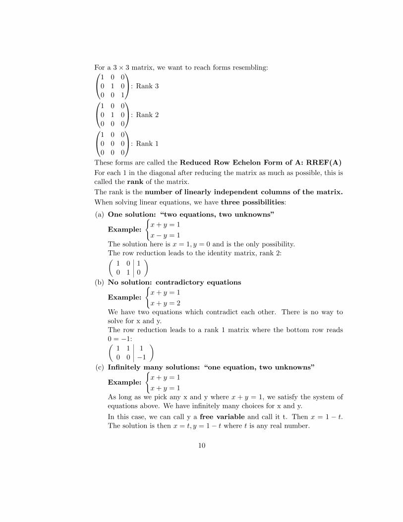
For a 3× 3 matrix, we want to reach forms resembling:1 0 00 1 00 0 1

: Rank 3

1 0 00 1 00 0 0

: Rank 2

1 0 00 0 00 0 0

: Rank 1

These forms are called the Reduced Row Echelon Form of A: RREF(A)

For each 1 in the diagonal after reducing the matrix as much as possible, this iscalled the rank of the matrix.

The rank is the number of linearly independent columns of the matrix.

When solving linear equations, we have three possibilities:

(a) One solution: “two equations, two unknowns”

Example:

{x+ y = 1

x− y = 1The solution here is x = 1, y = 0 and is the only possibility.The row reduction leads to the identity matrix, rank 2:(

1 0 10 1 0

)(b) No solution: contradictory equations

Example:

{x+ y = 1

x+ y = 2We have two equations which contradict each other. There is no way tosolve for x and y.The row reduction leads to a rank 1 matrix where the bottom row reads0 = −1:(

1 1 10 0 −1

)(c) Infinitely many solutions: “one equation, two unknowns”

Example:

{x+ y = 1

x+ y = 1As long as we pick any x and y where x + y = 1, we satisfy the system ofequations above. We have infinitely many choices for x and y.

In this case, we can call y a free variable and call it t. Then x = 1 − t.The solution is then x = t, y = 1− t where t is any real number.

10

For example, if we set x = 85, then y = 1− 85 = −84. If we set x = 0 theny = 1. The row reduction leads to:(

1 1 10 0 0

)4. Matrices as linear transformations

Matrices are representations of a linear transformation: the columns of thematrix are the results of the transformation applied to the basis vectors.

The equation Ax = b can be thought of as using the linear function A totransform the vector x into b.

A linear transformation is a map A : V →W such that

A(cv) = cL(v), A(v +w) = A(v) +A(w) for all vectors v, w, in V and scalars c.

Examples: Rotation, scaling, reflecting, shears, projections.

5. Example of the effect of A

Suppose A =

(1 23 4

)The basis vectors are:

e1 =

(10

)e2 =

(01

)The matrix A tells us that:

A · e1 =

(13

)and: A · e2 =

(24

)(

13

)is the result of applying the transformation A to e1.(

24

)is the result of applying the transformation A to e2.

6. Examples of 2D transformations as matrices:

(a) Do nothing: Av = v:

A is the identity matrix:

(1 00 1

)A · e1 =

(10

)and: A · e2 =

(01

)=⇒ Ae1 = e1, Ae2 = e2.The vectors remain unchanged after the transformation.

(b) Scale by a factor of c: Av = cv

A is a scaled identity matrix:

(c 00 c

)11

A · e1 =

(c0

)and: A · e2 =

(0c

)=⇒ Ae1 = ce1, Ae1 = ce2The components of the vectors are each scaled by a factor of c after thetransformation, stretching or shrinking them accordingly.

(c) Reflect about the y-axis:

The matrix A takes a special form: A =

(−1 00 1

)If this transformation reflects the vectors about the y-axis:Then the x-components change sign and the y-components are un-changed:

The first entries of each vector must change sign and second entriesof each vector are unchanged:In 2 dimensions:

The vector

(xy

)becomes the vector

(−xy

)Applying this to the basis vectors e1, e2:

A · e1 =

(−1 00 1

)(10

)=

(−10

)= −e1

A · e2 =

(−1 00 1

)(01

)=

(01

)= e2

(d) 90 degree counterclockwise rotation:Rotations for e1, e2:

e1 =

(10

)→(

0−1

)e2 =

(01

)→(

10

)The matrix must then be:

A =

(0 1−1 0

)It turns out that the following matrix represents counterclockwise rotationby any angle θ:

Q =

(cos(θ) sin(θ)− sin(θ) cos(θ)

)If θ = π

2 , we obtain the 90 degree rotation matrix A above.

(e) Matrix Multiplication as applying two transformations

Suppose A is a scaling matrix and B is a reflection matrix(about the y-axis). Thinking of AB(v) as a function composition A ◦ B, AB is theeffect of applying transformation B, then transformation A.

This means that AB(v) = A(B(v)): We reflect, then scale.

12

Applying this to e1:

(10

)→(−10

)→(−c0

)Applying this to e2:

(01

)→(−01

)→(

0c

)This means that AB =

(−c 00 c

)This is the full effect of reflecting about the y-axis, then scaling by c:

AB =

(c 00 c

)·(−1 00 1

)=

(−c 00 c

)That is:AB = scaling ◦ reflection

• Determinants

Properties of the determinant for matrices A,B that are n× n:

1. det(AB) = det(A) det(B)

2. det(cA) = cn det(A)

3. det(A+B) 6= det(A) + det(B) in general.

1× 1 determinant(a 1× 1 matrix is a single number)

det(a) = a

2× 2 determinant:

det

(a bc d

)=

∣∣∣∣a bc d

∣∣∣∣ = ad− bc

The determinant is really just the volume spanned by the parallelogramof the vectors obtained from the linear transformation A

The parallelogram formed by the vectors

e1 =

(10

), e2 =

(01

)is just a square sitting on the origin:

13

If A =

(a bc d

), e1, e2 become the vectors:

Ae1 =

(ac

), Ae2 =

(bd

)The area inside is ad− bc, the determinant.

14

In 3 dimensions, we have what is called a parallelopiped:

For a 3× 3 matrix, the determinant is:

det

a b cd e fg h i

= a

∣∣∣∣e fh i

∣∣∣∣− b ∣∣∣∣d fg i

∣∣∣∣+ c

∣∣∣∣d eg h

∣∣∣∣= a(ei− fh)− b(di− fg) + c(dh− eg).

This is the volume of the 3D shape above.

The determinant of A measures how much the area or volume of the shapechanges after applying the linear transformation A.

• Inverses: “Division” in the matrix world

A−1 is the inverse of A, essentially “ 1A” in matrix language.

Just as for a constant a · 1a = 1 if a 6= 0, for any invertible nxn matrix A,AA−1 = I

Also, A−1A = I.

A matrix is invertible if det(A) 6= 0

For a 2× 2 matrix, the expression looks like:

(a bc d

)−1=

d −c−b a

det(A) =

d −c−b a

ad−bc

For a 3×3 matrix, the inverse is significantly more complicated to compute, but stilltakes the form matrix

det(A)

Calculating Inverses by Row-Reduction

15

To find an inverse by row-reduction, we can row reduce an augmented matrix con-taining A on one side and the identity on the other until the A−1 on the left becomesthe identity and the identity on the right becomes the inverse that we need:

(A|I)→ (I|A−1)

• Example: Inverse by row-reduction(2 0 1 00 2 0 1

)12R1,

12R2−→(

1 0 12 0

0 1 0 12

)=⇒ A =

(2 00 2

)=⇒ A−1 =

(12 00 1

2

)Checking our work:

AA−1 =

(2 00 2

)(12 00 1

2

)=

(2(12) + 0 0 + 0

0 + 0 2(12)

)=

(1 00 1

)= I

In our transformation language:

AA−1 = I =⇒ Applying A−1, the reverse of the transformation A, then A itself isthe same as doing nothing:

In this example: Scaling vectors by 12 then scaling by 2 = same effect as doing nothing.

• Trace

The trace of a matrix Tr(A), is the sum of the diagonal entries:

Tr(A) = a11 + a22 + a33 + · · ·+ ann

For a 2× 2 matrix A =

(a bc d

), Tr(A) = a+ d.

• Trace Example:

Find the trace:

A =

(1 23 4

)Tr(A) = 1 + 4 = 5.

B =

1 2 34 5 67 8 9

Tr(B) = 1 + 5 + 9 = 15.

• Diagonal matrices/scaling transformations

A diagonal matrix takes the form:

16

D =

d1 0 0 · · · 00 d2 0 · · · 00 0 d3 · · · 0...

......

. . . 00 0 0 · · · dn

3× 3 case:

D =

d1 0 00 d2 00 0 d3

Special properties:

In the 3× 3 case:

1. Powers transfer through the diagonal elements:

D3 =

d31 0 00 d32 00 0 d33

2. The determinant is the product of the diagonal elements:

det{D} = d1 · d2 · d33. The inverse is the same matrix with reciprocal elements:

D−1 =

1d1

0 0

0 1d2

0

0 0 1d3

4. Diagonalization:

For a matrix A, if there exists an invertible matrix S such that we can find adiagonal matrix D such that A = S−1DS, we say that the matrix is similar toa diagonal matrix.

This is the same as saying that A is diagonalizable.

This is useful for computing powers of the matrix A:

A2 = A · A = (S−1DS)(S−1DS) = S−1D(SS−1)DS = S−1DIDS = S−1D2S.This means that Ak = S−1DkS for positive whole numbers k.

Diagonalizability also means that many properties of the diagonal matrixare shared such as linear independence of the rows and columns, eigenvaluesand eigenvectors(which are defined below).

17

• Eigenvalues and eigenvectors:

Eigenvalues are values λ (greek letter lambda) such that for a vector x 6= 0, Ax = λx.λ can be real or imaginary.

To find λ:

Ax = λx ⇐⇒ (A− λI)x = 0 ⇐⇒ det(A− λI) = 0

For a 2× 2 matrix:

(A− λI) =

(a bc d

)− λ

(1 00 1

)=

(a− λ bc d− λ

)To find λ, we compute:

det(A− λI) = det

(a− λ bc d− λ

)= 0

=⇒ (a− λ)(d− λ)− bc = 0

=⇒ λ2 − (a+ d)λ+ (ad− bc) = 0

This equation is sometimes called a characteristic equation.

This is equivalent to:

det(A) = λ2 − λTr(A) + det(A).

A convenient relationship.

Vectors x 6= 0 that have the aforementioned property are called eigenvectors and thecollection of eigenvectors is called the eigenspace of A.

Meaning in terms of transformations:

Eigenvectors are the vectors whose direction remains unchanged after a lineartransformation, however they may be scaled by a constant. Eigenvalues arethese scaling constants.

If there is a transformation that appears to have no directions among real-valuedvectors unchanged after a linear transformation, then the eigenvalues andeigenvectors are imaginary.

This means that there are infinitely many eigenvectors, but only finitely many direc-tions: many of the vectors are redundant since they are parallel to many others.

18

• Eigenvalue and eigenvector example:

Find the eigenvalues and eigenvectors of the following matrix:

A =

(−1 00 1

)1. Finding eigenvalues:

A− λI =

(−1− λ 0

0 1− λ

)Characteristic polynomial:

det(A− λI) = (−1− λ)(1− λ)− 0 · 0 = 0 =⇒ λ = 1,−1

Also, we could have used the formula from above:

det(A− λI) = λ2 − Tr(A)λ+ det(A) = λ2 − (−1 + 1)λ+ (−1 · 1− 1 · 0)

= λ2 − 1 = (λ− 1)(λ+ 1) = 0 =⇒ λ = 1,−1

The eigenvalues are 1,−1.

2. Finding eigenvectors:

Solve: (A− λI)v = 0 :

(−1− λ 0

0 1− λ

)(v1v2

)=

(00

)The vectors v =

(v1v2

)are the eigenvectors. Since the matrix A is 2 × 2, there

are at most 2 eigenvector directions(but infinitely many parallel eigenvectors):

λ = 1 :(−1− λ 0 0

0 1− λ 0

)=

(−1− 1 0 0

0 1− 1 0

)=

(−2 0 00 0 0

) −12R1−→(

1 0 00 0 0

)The first row reads 1v1 + 0v2 = 0 =⇒ v1 = 0.

Since the second row is all zeroes after the row reduction, the system has in-finitely many solutions. v2 can be any real number, it is a free variable.

If we call v2 = t, then we have v =

(0t

)= t

(01

).

This represents any and all possible eigenvectors:

(01

),

(02

),

(03

), ... etc

All the vectors are parallel to

(01

), which means we can treat this as our single

eigenvector: v1 =

(01

).

Repeating this for λ = −1:

λ = −1 :(−1− λ 0 0

0 1− λ 0

)=

(−1− (−1) 0 0

0 1− (−1) 0

)=

(0 0 00 2 0

)19

12R2−→(

0 0 00 1 0

)Similarly, v1 = t, v2 = 0.

The eigenvectors take the form:

(t0

)= t

(10

). They are all parallel to

(10

).

=⇒ v2 =

(01

).

3. Final solution:

The eigenvalues and eigenvectors of the matrix A =

(−1 00 1

)are

λ1 = 1 with eigenvector v1 =

(01

)and λ2 = 1 with eigenvector v2 =

(10

).

4. Solution in terms of linear transformations:

A =

(−1 00 1

). From earlier, we saw that this matrix represents rotation about

the y-axis.

The eigenvectors are the vectors whose directions are unchanged by the trans-formation aside from scaling by a constant.

There are two possibilities:

(a) The vector has no x-component: It is parallel to

(01

), reflecting about

the y-axis leaves it unchanged(scales it by 1).

This means that

(01

)is the eigenvector direction corresponding to the eigen-

value 1.

(b) The vector has only an x-component: It is parallel to

(10

), reflecting

about the y-axis flips the vector(scales it by -1)

This means that

(10

)is the eigenvector direction corresponding to the eigen-

value -1.

Any two dimensional vectors not parallel to these two will have different behaviorafter the reflection.

For example, the vector

(11

)becomes

(−11

). Reflecting this vector has the

same effect as rotating it by 90 degrees counterclockwise.

20

The following theorem somewhat summarizes our earlier results:

• The Fundamental Theorem of Invertible Matrices

For a n× n matrix A, the following are equivalent:

1. A is invertible.

2. det(A) 6= 0

3. Ax = 0 ⇐⇒ x = 0

4. Ax = b has a unique solution.

5. A has n linearly independent eigenvectors.

6. A has linearly independent rows and columns.

7. Rank(A) = n

’

• Application of the Fundamental Theorem

Let’s take another look at the previous example:

Determine whether or not the vectors a =

(21

),b =

(03

)are linearly independent.

Applying the above theorem, all we need to know is whether or not the matrixcontaining these vectors as columns is invertible.

A =

(2 01 3

)Since det(A) = 2(3) − 0(1) = 6 6= 0, A is invertible. Since part 2 is satisfied, so ispart 6. The columns of the matrix are linearly independent, therefore the columnvectors are as well.

• Another application:

Determine whether or not the following vectors are linearly independent. If not, finda linear relation between the vectors. If the vectors form the columns of a matrix,what would its rank be?

v1 =

111

, v2 =

1−12

, v3 =

314

Applying part 6, we can arrange the columns into a matrix and see whether or notthe matrix is invertible(part 1) or has full rank(part 7).

Consider the matrix A =

1 1 31 −1 11 2 4

21

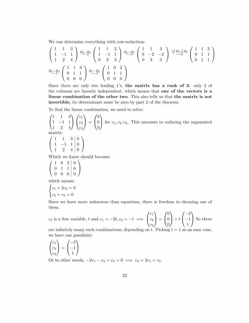
We can determine everything with row-reduction: 1 1 31 −1 11 2 4

R3−R2−→

1 1 31 −1 10 3 3

R2−R1−→

1 1 30 −2 −20 3 3

−12R2,

13R3−→

1 1 30 1 10 1 1

R3−R2−→

1 1 30 1 10 0 0

R1−R2−→

1 0 20 1 10 0 0

Since there are only two leading 1’s, the matrix has a rank of 2: only 2 ofthe columns are linearly independent, which means that one of the vectors is alinear combination of the other two. This also tells us that the matrix is notinvertible, its determinant must be zero by part 2 of the theorem.

To find the linear combination, we need to solve:1 1 31 −1 11 2 4

c1c2c3

=

000

for c1, c2, c3. This amounts to reducing the augmented

matrix: 1 1 3 01 −1 1 01 2 4 0

Which we know should become: 1 0 2 0

0 1 1 00 0 0 0

which means:{c1 + 2c3 = 0

c2 + c3 = 0

Since we have more unknowns than equations, there is freedom in choosing one ofthem.

c3 is a free variable, t and c1 = −2t, c2 = −t =⇒

c1c2c3

=

000

+ t

−2−11

So there

are infinitely many such combinations, depending on t. Picking t = 1 as an easy case,we have one possibiity:c1c2c3

=

−2−11

Or in other words, −2v1 − v2 + v3 = 0 =⇒ v3 = 2v1 + v2.

22

We can verify:

v1 =

111

, v2 =

1−12

, v3 =

314

2v1 + v2 = 2

111

+

1−12

=

2 + 12− 12 + 2

=

314

= v3.

So the vectors are linearly dependent. We are done.

A resource with vivid animations highlighting some of the above concepts:3Blue1Brown from KhanAcademy:

https://www.youtube.com/playlist?list=PLZHQObOWTQDPD3MizzM2xVFitgF8hE_ab

23