Linear Algebra and its Applications 471 (2015) 500–530

Contents lists available at ScienceDirect

Linear Algebra and its Applications

www.elsevier.com/locate/laa

Solving piecewise linear systems in abs-normal form

Andreas Griewank ∗, Jens-Uwe Bernt, Manuel Radons, Tom StreubelDepartment of Mathematics, Humboldt-Universität zu Berlin, Germany

a r t i c l e i n f o a b s t r a c t

Article history:Received 21 November 2013Accepted 18 December 2014Available online xxxxSubmitted by H. Fassbender

MSC:90C3390C5649J5265F99

Keywords:Switching depthSign real spectral radiusCoherent orientationGeneralized JacobianSemismooth NewtonPartial contractivityComplementary system

With the ultimate goal of iteratively solving piecewise smooth (PS) systems, we consider the solution of piecewise linear (PL) equations. As shown in [7] PL models can be derived in the fashion of automatic or algorithmic differentiation as local approximations of PS functions with a second order error in the distance to a given reference point. The resulting PL functions are obtained quite naturally in what we call the abs-normal form, a variant of the state representation proposed by Bokhoven in his dissertation [27]. Apart from the tradition of PL modelling by electrical engineers, which dates back to the Master thesis of Thomas Stern [26] in 1956, we take into account more recent results on linear complementarity problems and semi-smooth equations originating in the optimization community [3,25,5]. We analyze simultaneously the original PL problem (OPL) in abs-normal form and a corresponding complementary system (CPL), which is closely related to the absolute value equation (AVE) studied by Mangasarian and Meyer [14] and a corresponding linear complementarity problem (LCP). We show that the CPL, like KKT conditions and other simply switched systems, cannot be open without being injective. Hence some of the intriguing PL structure described by Scholtes in [25] is lost in the transformation from OPL to CPL. To both problems one may apply Newton variants with appropriate generalized Jacobians directly computable from the abs-normal representation. Alternatively, the CPL can be solved by Bokhoven’s modulus method and related fixed point iterations.

* Corresponding author.E-mail addresses: griewank@math.hu-berlin.de (A. Griewank), berntj@math.hu-berlin.de

(J.-U. Bernt), radons@math.hu-berlin.de (M. Radons), streubel@math.hu-berlin.de (T. Streubel).

http://dx.doi.org/10.1016/j.laa.2014.12.0170024-3795/© 2015 Elsevier Inc. All rights reserved.

A. Griewank et al. / Linear Algebra and its Applications 471 (2015) 500–530 501

We compile the properties of the various schemes and highlight the connection to the properties of the Schur complement matrix, in particular its partial contractivity as analyzed by Rohn and Rump [23]. Numerical experiments and suitable combinations of the fixed point solvers and stabilized generalized Newton variants remain to be realized.

© 2015 Elsevier Inc. All rights reserved.

1. Introduction and motivation

In many applications one encounters piecewise smooth (PS) functions that can be approximated locally with second order error by piecewise linear (PL) functions. In this paper we will assume throughout that all functions are continuous and thus, in fact, Lip-schitz continuous. However, an extension to piecewise linear but possibly discontinuous problems should be in the back of our minds before we settle on data structures and interfaces. Discontinuous solution operators may arise for example, if one considers least squares problems defined by piecewise linear systems of equations.

The process of piecewise linearization of a piecewise smooth function F : D ⊂ Rn �→

Rm given by an evaluation procedure was described in [7]. The key assumption is that all

nonsmoothness can be cast in terms of the absolute value function | · |. Then piecewise linearization can be achieved in the style of algorithmic differentiation [9] by simply replacing all smooth elemental functions by their tangent line or plane (in case of binary operations or special functions) and the absolute value function by itself.

In contrast to conventional notions of differentiation one does not obtain a collection of derivative vectors or matrices at a given reference point x. Rather one arrives at a procedure for evaluating an incremental PL function ΔF (x, Δx) : D × R

n �→ Rm for

which

F (x + Δx) = F (x) + ΔF (x,Δx) + O(‖Δx‖2).

Here the error term ‖Δx‖2 is uniform on compact subsets of D − x. This means that ΔF (x, Δx) is a candidate for a nonsingular uniform Newton approximation in the sense of [5], although the local homeomorphism property is by no means guaranteed.

Throughout this paper we will only be concerned with the properties of the piecewise linearized function. We will also drop the decomposition into F (x) and the increment ΔF (x, Δx) and consider a globally defined piecewise linear continuous (PL) mapping

F (x) : Rn �→ R

m.

Like for the (possibly) underlying nonsmooth mapping, our ultimate purpose is to solve certain basic numerical tasks, in particular (un)constrained optimization, equation solv-ing, and the numerical integration of dynamical systems.

502 A. Griewank et al. / Linear Algebra and its Applications 471 (2015) 500–530

Here we will consider, for m = n, the problem of solving the formally well determined system of equations

F (x) = 0 ∈ Rn, for x ∈ R

n. (1)

The paper is organized as follows: In Section 2 we introduce PL functions F in abs-normalform, a term that was apparently introduced by Barton and Khan in a more general non-linear setting [11]. In Section 3 we describe the resulting polyhedral structure and give an explicit procedure for calculating generalized Jacobians of F , which were shown in [11,12,7] to be conically active limiting Jacobians of the underlying piecewise smooth func-tion, whenever F was obtained as its piecewise linearization. In Section 4 we examine the relation between the global properties of bijectivity and coherent orientation, which coincide under certain rather generic conditions. Section 5 discusses sufficient conditions for the global convergence of the generalized Newton method, which is often referred to as semi-smooth Newton. In Section 6 we unfold the system by elevating the intermedi-ate switching variables to the status of full variables. As is the case for the unfolding of smooth singular equations [8], in this process some regularity is gained, but some information is also lost. The resulting system, that we call the complementary piecewise linear system (CPL), is always simply switched and as shown in Section 7, it can be solved by two different fixed point methods and several variants of generalized Newton. Finally, the complementary system can also be rewritten as a linear complementarity problem [3] with coherent orientation being equivalent to the P-matrix property. The final Section 8 summarizes our results and provides an outlook to further developments.

2. The abs-normal form

As also observed by Scholtes in [25] any piecewise linear scalar function f : Rn �→ R

has a so-called max-min representation

f(x) = max1≤i≤l

minj∈Mi

a�j x + bj

where the l index sets Mi are contained in {1, 2 . . . k} for some k ∈ N and the ai ∈ Rn,

bi ∈ R are constant coefficients. For a PL vector function F : Rn �→ Rm each one of

the m component functions can be represented in the same way. Moreover, using the equivalences

max(u,w) = 12(u + w + |u− w|

)and min(u,w) = 1

2(u + w − |u− w|

)

one can express all min and max expressions in terms of s ≥ 0 absolute value func-tions |zi|, whose arguments zi are called switching variables.

A. Griewank et al. / Linear Algebra and its Applications 471 (2015) 500–530 503

Observing that each zi is an affine function of absolute values |zj| with j < i and the independents xk for k ≤ n, one arrives at an abs-normal representation

[z

y

]=

[c

b

]+[Z L

J Y

] [x

|z|

]. (2)

Here the two vectors and four matrices specifying the function F have the formats

c ∈ Rs, Z ∈ R

s×n, L ∈ Rs×s, b ∈ R

m, J ∈ Rm×n, Y ∈ R

m×s.

The matrix L is strictly lower triangular so that for given x the components of z = z(x)and thus |z| can be unambiguously computed one by one. Specifically, we have Lij = 0exactly if zi depends directly on |zj | so that there is an edge between the nodes jand i in the corresponding data dependency graph. This graph is always acyclic and the components of x, y and z represent its roots, leaves and internal vertices, respectively.

Of course, the representation (2) is by no means unique for a given mapping F . One would naturally strive to make the representation as concise as possible in some sense. Excluding incidental cancellations, we find that the smallest integer ν ≤ s for which

Lν = 0

corresponds to the maximal number of internal nodes in any chain in the data dependency graph. We will call this the switching depth and consider it as key measure of the combinatorial difficulty of the function F . In this terminology, F is fully linear exactly if ν = 0 with s = 0 and thus z, Z, and L are empty. We will refer to this limiting situation as the smooth case. We will call F simply switched if ν = 1, a situation that arises for example in complementarity problems, where none of the nonsmooth elements are superimposed. We conjecture that, for any PL mapping F : Rn �→ R

m, there is an abs-normal representation with a switching depth ν ≤ ν(n) = 2n − 1.

Formulations similar to our abs-normal form have been used for a long time in the engineering literature. In [28,13] several classes of PL models are compared, Chua1 has switching depth 1 and Grü as well as Bokh2 are limited to switching depth 2. It is shown there that all of them are specializations of the model Bokh1, which is a priori implicit in that evaluating y for given x requires the solution of an LCP with a system matrix D. However, if D is also lower triangular solving the LCP requires simply a forward substitution. Then, provided D is nonsingular, the intermediate variables z can be rescaled such that D−I and consequently the Möbius transform L = (I+D)−1(I−D)of D become strictly lower triangular. L then defines an abs-normal form equivalent to the Bokh1 system.

Mangasarian and Meyer also observed in [14] the connection between LCPs and what they call an absolute value equation (AVE), the concept of which is closely related to our complementary system (CPL). We will partly replicate and strengthen their result.

504 A. Griewank et al. / Linear Algebra and its Applications 471 (2015) 500–530

As we have noticed, the abs-normal form is general enough to represent all continuous PL functions, so we will not use the even greater generality of the implicit Bokh1 model.

In the more mathematical literature, piecewise linear systems are often specified by linear pieces on simplices defined by systems of linear inequalities. These approaches may also be interpreted as conjunctive programming or mixed integer nonlinear programs (MINLP) as in [6]. However, their representations tend to be of combinatorial complexity and highly redundant, whereas the abs-normal form is stable and completely free of redundancy. In particular, any perturbation of the four matrices Z, L, J and Y that preserves the strict lower triangularity of L again unambiguously defines a continuous PL function y = F (x).

In the simply switched case we have z = c + Zx, which means that potential kinks occur in the union of the s hyperplanes zi(x) = ci + e�i Zx = 0 for i = 1 . . . s. We will then say that the kinks satisfy the linear independence kink qualification LIKQ if the normals of the hyperplanes intersecting at some point x are always linearly independent. This implies in particular that the vector z = c + Zx can never have more than nvanishing components. LIKQ is implied by all square submatrices of [c, Z] ∈ R

s×(1+n)

of order min(s, n + 1) being nonsingular. That slightly stronger condition is for example satisfied if c = 1 is the vector of ones and Z = (λj

i )i=1...sj=1...n is a Vandermonde matrix at

distinct abscissas λi for i = 1 . . . s. Consequently, the polynomial P (c, Z) formed by the product of the determinants of all maximal square submatrices [c, Z] does not vanish at the Vandermonde choice and the same is true for almost all matrices [c, Z] ∈ R

s×(1+n). In other words, LIKQ is a generic property, like linear independence of active constraints in linear optimization (LOP).

2.1. The Rosette example

To highlight the possible properties of PL functions we take a look at the following class of examples. Positively homogeneous functions in two variables are uniquely defined by their values on the unit circle, which must be 2π periodic functions of the polar angle ϕ(x) = arctan(x1, x2). More specifically, we assume that we have a monotonically growing sequence of angles

0 = ϕ0 < ϕ1 < . . . < ϕn−1 < ϕn = 2π

and corresponding values

(ψi)i=0...n with ψn − ψ0 = 2pπ for p ∈ N.

By suitable subdivisions we can ensure that the increments ϕi−ϕi−1 and |ψi−ψi−1| are all less than π. Then there exists a homogeneous piecewise linear function F : R2 �→ R

2

such that

F (cosϕi, sinϕi) = (cosψi, sinψi) for i = 0 . . . n.

A. Griewank et al. / Linear Algebra and its Applications 471 (2015) 500–530 505

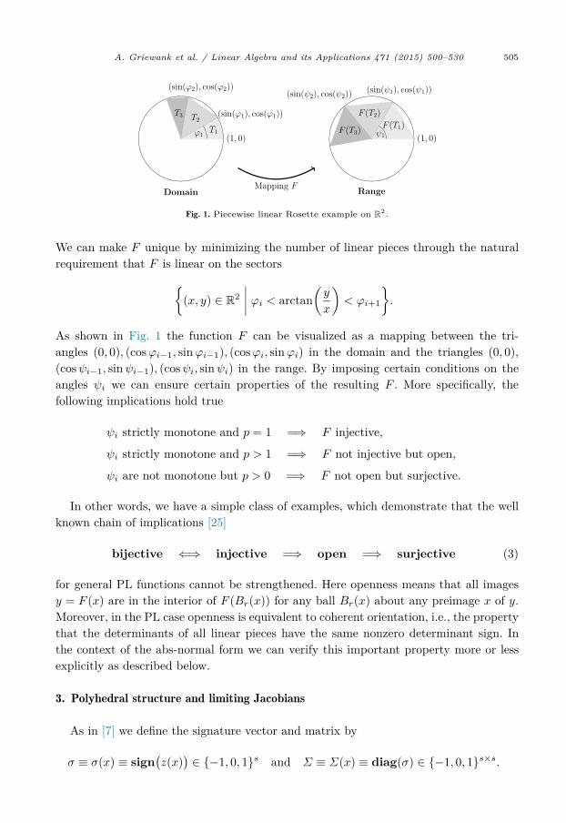
Fig. 1. Piecewise linear Rosette example on R2.

We can make F unique by minimizing the number of linear pieces through the natural requirement that F is linear on the sectors

{(x, y) ∈ R

2∣∣∣∣ ϕi < arctan

(y

x

)< ϕi+1

}.

As shown in Fig. 1 the function F can be visualized as a mapping between the tri-angles (0, 0), (cosϕi−1, sinϕi−1), (cosϕi, sinϕi) in the domain and the triangles (0, 0),(cosψi−1, sinψi−1), (cosψi, sinψi) in the range. By imposing certain conditions on the angles ψi we can ensure certain properties of the resulting F . More specifically, the following implications hold true

ψi strictly monotone and p = 1 =⇒ F injective,

ψi strictly monotone and p > 1 =⇒ F not injective but open,

ψi are not monotone but p > 0 =⇒ F not open but surjective.

In other words, we have a simple class of examples, which demonstrate that the well known chain of implications [25]

bijective ⇐⇒ injective =⇒ open =⇒ surjective (3)

for general PL functions cannot be strengthened. Here openness means that all images y = F (x) are in the interior of F (Br(x)) for any ball Br(x) about any preimage x of y. Moreover, in the PL case openness is equivalent to coherent orientation, i.e., the property that the determinants of all linear pieces have the same nonzero determinant sign. In the context of the abs-normal form we can verify this important property more or less explicitly as described below.

3. Polyhedral structure and limiting Jacobians

As in [7] we define the signature vector and matrix by

σ ≡ σ(x) ≡ sign(z(x)

)∈ {−1, 0, 1}s and Σ ≡ Σ(x) ≡ diag(σ) ∈ {−1, 0, 1}s×s.

506 A. Griewank et al. / Linear Algebra and its Applications 471 (2015) 500–530

This vector maps Rn into {−1, 0, 1}s and represents the control flow in our calculation. As an aside we note that all possible sign combinations must indeed occur if Z is surjective, which requires s ≤ n so that there may actually occur 3s different signatures. As in [7]one can verify that the corresponding sets

Pσ ≡{x ∈ R

n : σ(x) = σ}

are relatively open and convex polyhedra in Rn. Being inverse images they are mutually disjoint and span the whole domain Rn. By continuity it follows that Pσ must be open (possibly empty) if σ is definite in that all its components are nonzero. In degenerate situations there may be some indefinite σ for which Pσ is nevertheless open. Throughout we call Pσ and σ essential if Pσ is open and nonempty.

The limiting Jacobian ∂LF (x) at some x ∈ Rn, i.e., the limits of all proper Fréchet

derivatives in its neighborhood, is in the PL case simply the finite set

∂LF (x) = {Jσ : x ∈ Pσ with σ essential}.

The Clarke generalized Jacobian is the convex hull ∂F (x) = conv(∂LF (x)). In general it will be quite difficult to calculate all elements of the generating set ∂LF (x) and we will usually shy away from that combinatorial effort.

3.1. Explicit Jacobian representation

On all essential Pσ we find that |z| = Σz, so that the first equation in (2) yields

(I − LΣ)z = c + Zx and z = (I − LΣ)−1(c + Zx).

Notice that due to the strict triangularity of LΣ the inverse of (I − LΣ) is well defined and polynomial in the entries of L. Moreover, due to the structural nilpotency degree νof L we obtain the Neumann expansion

(I − LΣ)−1 = I + LΣ + (LΣ)2 + · · · + (LΣ)(ν−1). (4)

In the simply switched case ν = 1 we have L = 0 and thus the expansion reduces to I−1 = I. When ν = 2, we have the linear inverse (I − LΣ)−1 = I + LΣ. Substituting this expression into the second part of (2) we obtain the local representation:

Proposition 3.1. On all essential Pσ the dependents y can be directly expressed in terms of x, namely as

y = b + Y Σ(I − LΣ)−1c + Jσx with Jσ = J + Y Σ(I − LΣ)−1Z. (5)

Here Jσ is the Jacobian of F restricted to Pσ. It reduces to Jσ = J + Y ΣZ for simply switched problems (ν = 1) and to J for smooth problems (ν = 0).

A. Griewank et al. / Linear Algebra and its Applications 471 (2015) 500–530 507

3.2. Polynomial escape

Computing generalized Jacobians Jσ according to (5) is quite simple, once an essential signature σ and thus the corresponding diagonal Σ are known. To find, for a given x, some essential σ with the closure Pσ containing x one may use the following trick, which we like to call polynomial escape. Due to piecewise linearity the complement Cof all essential Pσ is contained in the union of finitely many hypersurfaces. Hence, no polynomial path of the form

x(t) ≡ x +n∑

i=1eit

i with det[e1, e2, . . . , en] = 0, for ei ∈ Rn

can be contained in C. In other words, we find for some σ and t > 0 that x(t) ∈ Pσ for all t ∈ (0, t). The corresponding σ can be computed by lexicographic differentiation as introduced by Nesterov [15] and described in a little more detail in [7]. There it is also shown that any such Jσ is in fact a generalized Jacobian of the underlying nonlinear function if F was obtained by piecewise linearization. Finally, by suitably selecting e1 =d = 0, one can make sure that the generalized Jacobian obtained is active in a cone containing the given direction d at least in its closure.

4. Coherent orientation and injectivity

As in the smooth case, the determinants of the Jacobians Jσ are of crucial importance for the properties of the PL function F : Rn → R

n. It is called coherently oriented if all its Jacobians have the same nonzero determinant sign. As stated for example in [25], the central property openness in the chain (3) is, for PL functions, equivalent to coherent orientation. For simply switched F , like for example all KKT systems of QOPs, we have essentially the same situation as in the affine case, namely bijectivity follows already from coherent orientation and LIKQ.

Proposition 4.1. If F is simply switched in that L = 0 and its kinks satisfy LIKQ then F is bijective if and only if it is coherently oriented.

Proof. If F is bijective it follows from Scholtes’ chain of implications (3) that it is already coherently oriented. For the inverse direction: On the basis of the mean value theorem, see Prop. 7.1.16 in [5], Clarke showed that F has an inverse function near some point xif all elements of the generalized Jacobian ∂F (x) are nonsingular. At all points where Fis differentiable this follows from the assumed coherent orientation. At all other points a certain number of m ≤ s components of σ vanish, which means in the simply switched case that the s-vector c + Zx has m zero components. In fact, it may contain at most m ≤ n zeros since otherwise a corresponding (n +1) × (n +1) sub-matrix of [c, Z] would have the nonzero null vector (1, x�)� ∈ R

n+1. Without loss of generality we may assume

508 A. Griewank et al. / Linear Algebra and its Applications 471 (2015) 500–530

that exactly the first m ≤ n components of z = z(x) vanish. The remaining ones will keep their sign in a sufficiently small neighborhood of x. Due to the linear independence of the first m rows of Z we can find arbitrarily small perturbations Δx ∈ R

n such that the first m components of c +Z(x +Δx) have any one of 2m sign patterns. Correspondingly, the first m components of the signature vector σ ∈ R

s attain any {−1, 1} pattern on some open domain whose closure contains the given points x. Hence, ∂F (x) contains all matrices Jσ = J + Y ΣZ where the last s − m components of Σ are fixed and the first m may be +1 or −1. By assumption, all these Jσ have the same determinant sign. Changing just one σi ∈ {−1, 0, 1} of the first m components continuously from −1 to +1corresponds to a rank one change in the corresponding matrix Jσ, whose determinant varies linearly with respect to σi and therefore cannot change signs in between. Thus the Jσ along all edges have the same determinant signs, which are inherited by the ones on the face and so on. Therefore, we have shown that all generalized Jacobians are nonsingular so that F is everywhere locally injective and also globally injective. �Lemma 4.2. Any F satisfying the assumptions of the proposition is stably coherently ori-ented in that all modifications generated by small perturbation of [c, Z] are also coherently oriented.

Proof. We firstly note that each open polyhedron of the original system is a simplex whose vertices are intersections of exactly n + 1 linearly independent hypersurfaces. Hence for sufficiently small perturbations of the data each of them persist and remain nondegenerate. Moreover, the determinant of the also continuously varying Jacobians maintain the same sign. Now suppose some arbitrarily small perturbations had an ad-ditional open polyhedron, for which we may assume without loss of generality the same definite signature σ, due to the finiteness of the whole situation. Then the corresponding polyhedron Pσ of the original problem must be nonempty but nonopen. That means the linear inequalities active at any one of its elements must be linearly dependent in violation of LIKQ. �

The converse is not true, since one may modify any coherently oriented F that vio-lates LIKQ at x into one that is stably coherently oriented by adding a suitable multiple α of the identity so that F (x) becomes F (x) + αx. This modification does not affect z and thus the lack of LIKQ. As we have seen the Rosette example may be open but not injective, which is not surprising since it has the switching depth 2 and is not sta-bly coherently oriented. Just assuming stable coherent orientation, we find that all the small perturbations satisfying LIKQ are injective and F , as the limit of such bijective perturbations, inherits this property by the proposition following the lemma below.

Lemma 4.3. Let D ⊆ Rn be open, and let {Fk} be a sequence of continuous injective maps

Fk : D → Rn which converges uniformly on compact sets to F : D → R

n. Then for every x0 ∈ D and every ε > 0 with Bε(x0) ⊆ D there exists k0 such that F (x0) ∈ Fk(Bε(x0))for all k ≥ k0.

A. Griewank et al. / Linear Algebra and its Applications 471 (2015) 500–530 509

Proof. Let y0 := F (x0). Since F−1(y0) is discrete, we can choose r > 0 such that B2r(x0) ⊆ D and B2r(x0) ∩ F−1(y0) = {x0}. After decreasing r if necessary, we can assume r ≤ ε for the given ε. Write Ω := Br(x0). Then y0 /∈ F (∂Ω), where ∂Ω is the border of Ω in the sense of [19], hence, dist(y0, F (∂Ω))/2 =: δ > 0 (note that F (∂Ω) is compact since F is again continuous). Choose k′ such that yk := Fk(x0) ∈ Bδ(y0) for all k ≥ k′. Choose k0 ≥ k′ such that ‖(F − Fk)|∂Ω‖∞ < δ for all k ≥ k0. Then, for each of these k, we have

dist(y0, Fk(∂Ω)

)≥ dist

(y0, F (∂Ω)

)−

∥∥(F − Fk)|∂Ω∥∥∞ > 2δ − δ = δ

and, consequently, Bδ(y0) ⊆ Rn \ Fk(∂Ω). Because of yk ∈ Bδ(y0), the points y0 and yk

lie in the same connected component of Rn \ Fk(∂Ω). Therefore we have

d(Fk, Ω, y0) = d(Fk, Ω, yk)

where d denotes the Brouwer degree (see e.g., [24]). The right-hand side of this equation is ±1 because Fk|

Ωis an injective continuous map from a compact set to a Hausdorff

space, hence, a homeomorphism onto its image. Thus, d(Fk, Ω, y0) = ±1 = 0 and, therefore, y0 ∈ Fk(Ω) for all k ≥ k0. The statement of the lemma now follows from Ω = Br(x0) ⊆ Bε(x0). �Proposition 4.4. Let {Fk} be defined as in Lemma 4.3. Assume that the preimage F−1(y) ⊆ D is discrete for every y ∈ im(F ). Then F is injective.

Proof. The proposition follows immediately by contradiction. Suppose there were x1 = x2 in D with F (x1) = F (x2) =: y0. Choose ε > 0 small enough such that Bε(x1)and Bε(x2) are disjoint subsets of D. Let k1, k2 be as in Lemma 4.3, that is, such that y0 ∈ Fk(Bε(xi)) for all k ≥ ki, i = 1, 2. Then y0 ∈ Fk(Bε(x1)) ∩ Fk(Bε(x2)) for every k ≥ max{k1, k2}, contradicting injectivity of the Fk. �

Hence we obtain the following strengthening of Proposition 4.1

Corollary 4.5. If F is simply switched and stably coherently oriented in that all small perturbations have this property, then it is bijective.

The simply switched one-dimensional example F (x) = x −|x −ζ| +|x +ζ| is monotonically growing and thus coherently oriented if ζ ≤ 0 but for ζ > 0 it has a slope of −1 in a small interval about the origin. Hence, for the limiting case ζ = 0, where F (x) ≡ x, we have coherent orientation, but that property is lost for arbitrarily small ζ > 0. Nevertheless, the function is of course injective so that one might conjecture that for simply switched PL functions openness already implies injectivity.

510 A. Griewank et al. / Linear Algebra and its Applications 471 (2015) 500–530

However, that is not the case as shown by the instance of the Rosette example.

F (x) ≡[

|x1| − |x2|12 |x1 + x2| − 1

2 |x1 − x2|

]. (6)

It is simply switched and coherently oriented, but not injective since F is even, so that F (−x) = F (x). The LIKQ is violated since the four kinks {x1 = 0}, {x2 = 0}, {x1 = x2}and {x1 = −x2} all intersect at the origin. Moreover, one can see that the perturbations

Fε(x) ≡[

|x1 + ε| − |x2 + ε|12 |x1 + x2| − 1

2 |x1 − x2|

]

are no longer coherently oriented for ε = 0. More specifically, for ε > 0 we have

F ′ε =

[1 −10 −1

]at x =

[x1x2

]=

[−ε/2−ε/4

]

whose determinant is −1 so that we do not have stable coherent orientation.

5. Generalized Newton variants

If all elements of ∂LF (x∗) are nonsingular at some root x∗ ∈ F−1(0), it follows from the celebrated theorem of Qi and Sun [18] that the full step iteration

x+ = x− J−1σ F (x), with Jσ ∈ ∂LF (x) (7)

converges from all x0 sufficiently close to x∗. In fact, this result holds here trivially, since the iteration converges in one step from all points in the open neighborhood

Ω(x∗) ≡ {Pσ : x∗ ∈ Pσ}◦.

Of course, this means that all the combinatorial issues have already been resolved by the choice of x0. Much more interesting is the question under which conditions the full step Newton method (7) converges globally, i.e., from all initial points x0. Using the mean value theorem of Clarke stated for example as Prop. 7.1.16 in [5], one can establish the following global convergence result.

Proposition 5.1 (Full step convergence). Given x∗ ∈ F−1(0) the full step Newton method converges from all x0 ∈ R

n in finitely many steps to x∗ if, with respect to some induced matrix norm, either of the following contractivity assumptions is satisfied

∥∥I − J−1σ Jσ

∥∥ < 1, for all essential σ, σ, (8)

or

A. Griewank et al. / Linear Algebra and its Applications 471 (2015) 500–530 511

∥∥I − JσJ−1σ

∥∥ < 1, for all essential σ, σ. (9)

In either case the root {x∗} = F−1(0) is unique.

Proof. By the mean value theorem we derive from (7) the solution error recurrence

x+ − x∗ = x− x∗ − J−1σ A(x− x∗) =

[I − J−1

σ A](x− x∗)

where for some m ≥ 1 and λi ∈ R

A =m∑i=1

λiJσiwith

m∑i=1

λi = 1 and λi > 0.

With a similar convex combination A of limiting Jacobians we find for the residual

F (x+) = F (x) − AJ−1σ F (x) =

[I − AJ−1

σ

]F (x). (10)

If we can ensure reduction of either norm ‖x − x∗‖ or ‖F (x)‖ by a fixed factor that implies at least linear convergence to a root. Then we eventually must reach an iterate x such that ∂F (x) ⊂ ∂F (x∗). In the next step we would get x+ = x∗. By the triangle inequality and our assumption (8) it follows that

∥∥∥∥∥I − J−1σ

m∑i=1

λiJσi

∥∥∥∥∥ =

∥∥∥∥∥m∑i=1

λi

(I − J−1

σ Jσi

)∥∥∥∥∥ ≤m∑i=1

λi

∥∥I − J−1σ Jσi

∥∥ < 1.

Since the number of all Jacobians is finite, there is a global maximum of the term (8), which bounds the reduction factor ‖x+−x∗‖/‖x −x∗‖. Similarly, (9) yields a bound less than 1 on the ratio ‖F (x+)‖/‖F (x)‖. This completes the proof. �

The proposition deals with a special case of the general theory on nonsingular uniform Newton approximations in the sense of [5]. Now we will look for sufficient conditions for the contractivity properties (8) or (9) and thus global convergence of full step Newton and injectivity of F in terms of the abs-normal representation. To obtain an explicit expression for the inverses J−1

σ we will assume that the matrix J ∈ Rn×n representing

the smooth part of our function is nonsingular. Should that a priori not be the case we can use the identity

v =∣∣|v| + v

∣∣− |v|, for v ∈ R (11)

to shift terms between the smooth and nonsmooth parts without changing the map-ping F . However, for each modified entry we introduce two new switching variables and thus the abs-normal form and its various properties are significantly altered. In partic-ular, the switching depth may rise by two and the problem can no longer be simply switched. Now we obtain the convergence result.

512 A. Griewank et al. / Linear Algebra and its Applications 471 (2015) 500–530

Proposition 5.2. Assume that the abs-normal form of F has an invertible smooth part Jand that

ρ ≡∥∥J−1Y

∥∥p‖Z‖p < 1 − ‖L‖p.

Then generalized Newton converges in finitely many iterations from any x0 to the then unique solution x∗ if

ρ ≡ 2ρ(1 − ρ− ‖L‖p)(1 − ‖L‖p)

< 1. (12)

Moreover, the p-norms of both the solution error and the residual are reduced by the factor no greater than ρ at each iteration.

Proof. It follows from (5) that

∥∥I − J−1Jσ∥∥p≤

∥∥J−1Y∥∥p

∥∥(I − LΣ)−1∥∥p‖Z‖p ≤ ρ/

(1 − ‖L‖p

).

Hence we have by the Banach Perturbation Lemma that

∥∥J−1σ J

∥∥p

=∥∥[I − (

I − J−1Jσ)]−1∥∥

p≤ 1/

[1 − ρ/

(1 − ‖L‖p

)],

which immediately yields for any pair of essential signatures σ, σ

∥∥J−1σ J

∥∥p≤ 1 − ‖L‖p

1 − ρ− ‖L‖p. (13)

Furthermore we derive from (5) that

J−1[Jσ − Jσ] = J−1Y[Σ(I − LΣ)−1 −Σ(I − LΣ)−1]Z

= J−1Y[(I − ΣL)−1Σ −Σ(I − LΣ)−1]Z

= J−1Y (I − ΣL)−1[Σ(I − LΣ) − (I − ΣL)Σ](I − LΣ)−1Z

= J−1Y (I − ΣL)−1[Σ −Σ](I − LΣ)−1Z.

Now taking again norms and applying standard inequalities we find

∥∥J−1(Jσ − Jσ)∥∥p≤ 2ρ

(1 − ‖L‖p)2. (14)

By multiplication of (13) and (14), the last inequality ensures that both (8) and (9) are satisfied. �

A. Griewank et al. / Linear Algebra and its Applications 471 (2015) 500–530 513

5.1. Piecewise Newton

The conditions for the global convergence of full step Newton derived above are certainly rather strong and various globalizations like Ralph’s path search have been proposed. On the other hand, it was observed in [7] that coherent orientation implies that the fibers

[x0] ≡{x ∈ R

n : F (x) = λF (x0), 0 < λ ∈ R}

(15)

are, for almost all x0 ∈ Rn, bifurcation-free piecewise linear paths whose closure contains

a root of F . The other singular fibers may have bifurcations, but there is always a possibility to further reduce the residual towards a solution.

The question how this piecewise Newton method is best implemented needs further investigation, but numerical experiments are certainly encouraging [17]. There is a key difference between this piecewise Newton and damped Newton in that piecewise Newton is not based on just any limiting Jacobian at the current iterate, but on one that is indeed valid along the direction being taken. It cannot be guaranteed in the usual paradigm that an oracle evaluates at any x the residual F (x) and some limiting Jacobian ∂LF (x).

We may summarize the results of this fourth and fifth section in the following graph of implications:

Contractivity ⇒ Bijectivity =⇒ Openness ⇒ Surjectivity(⇐= if simply switched + stably coherently oriented)

The fact that the last two implications are not reversible in general was already demon-strated in Section 2 on the Rosette example, which is not simply switched. The possibility of failure for full step Newton on bijective problems can be seen in the Rosette example (6). With a right-hand side (1, −1) and a starting point (2, 1), Newton’s method begins to cycle immediately.

6. Schur complement and the complementary system

It turns out that we can eliminate x when the smooth part J is nonsingular.

Lemma 6.1. Provided that det(J) = 0, we have the Schur complement

S ≡ L− ZJ−1Y ∈ Rs×s

and in Pσ it holds that

det(Jσ) = det(J) det(I − SΣ).

Moreover, if this determinant is nonzero, the inverse of Jσ is given by

J−1σ = J−1 − J−1Y Σ(I − SΣ)−1ZJ−1. (16)

514 A. Griewank et al. / Linear Algebra and its Applications 471 (2015) 500–530

Proof. As Sylvester’s determinant theorem states det(I + AB) = det(I + BA)

det(Jσ)/ det(J) = det[I + J−1Y Σ(I − LΣ)−1Z

]= det

[I + ZJ−1Y Σ(I − LΣ)−1]

= det(I − LΣ)−1 det(I − LΣ + ZJ−1Y Σ

)= det(I − SΣ)

where we have used that the unitary lower triangular matrix I − LΣ has determi-nant 1. �

Whenever J dominates the other three submatrices, things are not too difficult, as we will see below. Notice that nonsingular linear transformations on the independents x and/or the dependents y leave the Schur complement completely unchanged. At least for (generalized) Newton variants we could therefore assume without loss of generality that J = I, although that does not seem to help all that much.

Rescaling the switching variables z by a positive diagonal matrix D would modify Zto DZ, Y to Y D−1 and replace L by the similarity transformation DLD−1, which is still strictly lower triangular. One can choose D such that the transformed DLD−1 is arbitrarily small in any one of the standard norms that are monotonic in the coordinates, but that may require a pretty wild scaling. More important is the Schur complement S, which would also be replaced by its similarity transformation DSD−1.

6.1. Conditions for coherent orientation

The condition that det(I−SΣ) be positive for all switching matrices Σ is sufficient for coherent orientation of F . An equivalent observation attributed to Rohn by Neumaier [16] is that for each 0 = x ∈ R

n there exists an index i such that e�i |Sx| < e�i |x|. Neumaier called this nonexpanding but we prefer the term partially contractive as it seems more descriptive. In addition to the ones provided by Rohn, Rump gave another equivalent characterization of partial contractivity namely that the sign real spectral radius

ρs0(S) ≡ max{ρ0(ΣS) : Σ ∈ diag{−1, 1}n

}

is less than 1. Here ρ0(S) ≤ ρ(S) denotes the real spectral radius of a square matrix, i.e., the largest modulus of any real eigenvalue of S ∈ R

n×n. The complex eigenvalues are ignored in this maximization, which makes ρ0(S) highly discontinuous with respect to S. Remarkably, ρs0(S) is again continuous in the entries of S and it vanishes exactly when S is permuted strictly triangular. This is true for the leading part L of our Schur complement so that we must have ρs0(S) < 1 when the additional term Y J−1Z is suffi-ciently small. In general, deciding whether ρs0(S) lies below a given bound is an NP hard problem. Rump also showed that the following property is sufficient, but not necessary for ρs0(S) < 1 and, thus, coherent orientation.

A. Griewank et al. / Linear Algebra and its Applications 471 (2015) 500–530 515

Definition 6.2. An abs-normal form of F is called smoothly dominant if

ρ ≡∥∥DSD−1∥∥

p< 1

for some p-matrix norm and some positive diagonal scaling D.

This condition was already used by Bokhoven in his dissertation [27]. Similarly, Man-gasarian and Meyer [14] wrote their absolute value equation Ax − |x| = b in terms of the inverse A = S−1. Assuming smooth dominance of A−1 for the special choice p = 2and D = I they showed unique solvability of the AVE. This can be shown directly us-ing the contractivity of what Bokhoven and his followers call the modulus algorithm as discussed below. First we will show that coherent orientation may be present even when all p-norms are substantially greater than 1, i.e., when the PL system is far from being smoothly dominant.

Lemma 6.3. There are matrices Sn ∈ Rn×n with signed real spectral radius ρs0(Sn) ≤ 0.9

for which all p norms ‖D−1n SnDn‖p with arbitrary diagonal scalings Dn > 0 are greater

than 1, for n ≥ 3 and furthermore limn ‖D−1n SnDn‖p = ∞.

Proof. Dropping the subscript n and abbreviating e ≡ (1 . . . 1)� ∈ Rn, I ∈ R

n×n we consider Rump’s example

S = 910 ·

(sign(j − i)

)i,j=1...n ∈ R

n×n with |S| = 910

(ee� − I

). (17)

Since, for any D = diag(d) ∈ Rn×n with (d > 0, componentwise)

∥∥DSD−1∥∥∞ =

∥∥D|S|D−1∥∥∞,

we obtain

109∥∥DSD−1∥∥

∞ =∥∥D(

ee� − In)D−1∥∥

∞ =∥∥Dee�D−1 − In

∥∥∞

≥∣∣∥∥Dee�D−1∥∥

∞ − ‖I‖∞∣∣ =

∣∣∣∣∣ max1≤j≤n

n∑i=1

didj

− 1

∣∣∣∣∣.

By elementary arguments one can see that the expression on the RHS attains its minimal value n − 1 when all dj are equal so that

∥∥DSD−1∥∥∞ ≥ 9

10(n− 1).

Now let x ∈ Rn be the unit vector ‖x‖∞ = 1 that maximizes the infinity norm

‖DSD−1x‖∞, such that

516 A. Griewank et al. / Linear Algebra and its Applications 471 (2015) 500–530

∥∥DSD−1∥∥p

= max‖x‖p=1

∥∥DSD−1x∥∥p

≥ ‖DSD−1x‖p‖x‖p

≥ ‖DSD−1x‖∞‖x‖p

.

Finally this yields by the equivalence of the vector norms ‖x‖p ≤ n1p ‖x‖∞ = n

1p

‖DSD−1x‖∞‖x‖p

≥ n− 1n

1p

n→∞−−−−→ ∞.

On the other hand, we know from [23] that the sign real spectral radius satisfies ρs0(S) =0.9 < 1 so that we have coherent orientation of F as asserted. �

To see that smooth dominance can also arise when ρ(|S|) > 1 let us consider the 2 ×2matrix

S = R

(π

2

)= 0.9√

2

(1 −11 1

).

It represents a rotation by π/2 followed by a contraction by 0.9. Then we have

‖S‖2 = 0.9 < 1 < 0.9√

2 = ρ(|S|

).

As a more interesting example for smooth dominance let us consider a problem

Tx + max(x, 0) = b, where T � 0

is symmetric positive definite, which is the stronger assumption used in [1]. (The max is meant componentwise.) Rewriting this problem in abs-normal form using max(x, 0) ≡(x + |x|)/2 we obtain

z = x and y = −b + (T + I/2)x + |z|/2.

This corresponds to c = 0, Z = I, L = 0, J = T + I/2, Y = I/2 and yields the Schur complement S = 0 −(T +I/2)−1/2 = −(I+2T )−1 ≺ 0. It is negative definite with spectral radius below 1. Hence, we have smooth dominance as ‖DSD−1‖2 < 1 for D = I. We have verified that the fixed point iteration suggested in (22) below converges when T is the usual second order divided difference stencil. However, it does so very slowly and applying the generalized Newton iteration (7) and equivalently (23), also advocated in [1] turns out to be much more effective.

An even stronger condition for smooth dominance and thus coherent orientation fol-lows from the well known result of Perron–Frobenius.

A. Griewank et al. / Linear Algebra and its Applications 471 (2015) 500–530 517

Lemma 6.4 (Perron–Frobenius scaling). Suppose that S and hence its componentwise modulus |S| is not permuted block-triangular. Then the spectral radius ρ(|S|) is positive and the corresponding eigenvector d ∈ R

n is strictly positive such that for D = diag(d)and e = (1 . . . 1) ∈ R

s

D−1Sd ≡ D−1SDe = ρ(|S|

)e =⇒

∥∥D−1SD∥∥∞ = ρ(|S|).

If ρ(|S|) = 0, the norm ‖D−1SD‖∞ can be made arbitrarily small.

Proof. It is well known that all components of the eigenvector d are positive if the corre-sponding eigenvalue ρ(|S|) is nonzero. Then we find immediately that e is the eigenvector associated with the largest eigenvalue of |S| for S = D−1SD, which in turn shows that ‖S‖∞ = ‖|S|‖∞ has the same value. If ρ(|S|) = 0, we can add εee� to |S| and apply the first observation to establish the second. �

According to the lemma, absolute contractivity, i.e. ρ(|S|) < 1, implies smooth dom-inance in the scaled infinity norm. Moreover, we may always similarity transform S by some diagonal D > 0 such that all rows of S ≡ D−1SD have the same l1 norm equaling ρ(|S|) = ρ(|S|). We will call this process equilibration. This may not work if S is reducible in that it is permuted block triangular, which can for example be tested by the algo-rithm given in [4]. In the reducible case the complementary system discussed below can be decomposed into several subsystems, to which our solution techniques can be applied successively. Consequently, we may assume from now on without loss of generality that the sparsity pattern of S is irreducible, which also implies ρs0(S) > 0. Alternatively, we can scale by the left Perron–Frobenius vector d of |S| to achieve ‖D−1SD‖1 = ρ(|S|) for D = diag(d), but that appears to be of little help here.

6.2. The complementary system

We will assume throughout that J is nonsingular, hence, that S is well defined and that a suitable scaling was applied to make some norm ‖S‖p small, if not necessarily less than one. So far we have looked at (2) as a system that defines a unique z ∈ R

s and thus a corresponding y for each x ∈ R

n via the first set of s triangular equations. Now suppose we have given a fixed target value y, which we can subsume into b, and compute for each z the corresponding value

x = x(z) ≡ −J−1(b + Y |z|). (18)

Substituting this result into the first equation we obtain for z the PL system

H(z) ≡ z − L|z| + ZJ−1Y |z| = (I − SΣ)z = c ≡ c− ZJ−1b. (19)

518 A. Griewank et al. / Linear Algebra and its Applications 471 (2015) 500–530

Provided S has the inverse A we may write equivalently

H(z) = z − S|z| = c ⇐⇒ Az − |z| = b ≡ Ac. (20)

Here the right hand side represents the absolute value equation of Mangasarian and Mayer [14]. They make the interesting observation that if A is sufficiently small then only strictly negative rights hand sides b lead to solutions. Moreover, according to their Proposition 6 these inverse image sets attain all possible 2n sign combinations, as is obvious for the limiting case −|z| = b, where A vanishes. Intuitively it would seem that such complete domination of the smooth part by the nonsmooth part makes little sense in a realistic model. Correspondingly, Mangasarian and Mayer also consider the situation, where A is sufficiently large or in our formulation S is sufficiently small, e.g. in the sense of smooth dominance.

Note that the generalized Jacobians (I − SΣ) of the complementary vector function H(z) all have the same determinant sign if and only if S is partially contractive and equivalently ρs0(S) < 1, which we encountered as a sufficient condition for the coherent orientation of F . Generally, F (x) must be coherently oriented if this is true for H(z), but the converse implication is usually not true. The reason is that while all possible sign combinations of z arise in the domain Rs of z, the switching variables z = z(x) are typically restricted to a Lipschitzian submanifold in Rs as x ranges over Rn.

Conversely, for any given z solving the lower part of (2) for x yields the corresponding value

z = z(x) ≡ G−1(c + Zx) with G(z) ≡ z − L|z|. (21)

As stated by Lemma 6.4 we can make any p-norm ‖L‖p of the strictly lower triangular matrix L as small as possible and in particular smaller than 1. Then the existence of G−1

follows not only from the triangularity of L but also the Banach fixed point theorem. Now we can observe that solutions of the original problem OPL and the complementary problem CPL correspond to each other.

Lemma 6.5 (One-to-one solution correspondence). Under our general assumptions with det(J) = 0 a point x∗ ∈ R

n is a solution of the OPL F (x) = 0 if and only if it is a fixed point of x(z(x)), which is in turn equivalent to z∗ = z(x∗) being a fixed point of z(x(z))and equivalently a solution of the CPL H(z) = c.

Proof. We have the equivalences F (x) = 0

⇐⇒ x = −J−1[b + Y |z|]

with z = c + Zx + L|z|⇐⇒ x = −J−1[b + Y |z|

]with G(z) = c + Zx

⇐⇒ x = −J−1[b + Y∣∣G−1(c + Zx)

∣∣]⇐⇒ x = x

(z(x)

)⇐⇒ z = z

(x(z)

)

A. Griewank et al. / Linear Algebra and its Applications 471 (2015) 500–530 519

⇐⇒ z = G−1(c + Zx) with x = −J−1(b + Y |z|)

⇐⇒ z = G−1(c− ZJ−1(b + Y |z|))

⇐⇒ G(z) = c− ZJ−1(b + Y |z|)

⇐⇒ z − L|z| = c− ZJ−1(b + Y |z|)

which is equivalent to H(z) = c defined in (19) as asserted. �We may interpret H(z) as a simply switched PL function in abs-normal form with

z ≡ x, Z = I = J , L = 0, and Y = −S. The Schur complement is then again 0 − I

I−1(−S) = S, which was to be expected. Since the LIKQ condition is satisfied, the complementary function H(z) is always bijective if and only if it is open, which happens exactly when ρs0(S) < 1.

7. Solving the complementary system CPL

In view of Lemma 6.5 we can hope that the largely equivalent fixed point iterations x+ = x(z(x)) and z+ = z(x(z)) defined by (21) and (18) lead to convergence. As it turns out it is a little easier to establish convergence of the coupled iteration with respect to the z-component and the x-component must then converge to its own fixed point by continuity.

Proposition 7.1. The Block Seidel iteration z+ = z(x(z)) converges from all z0 to the unique fixed point z∗ if in some p-norm

‖S − L‖p + ‖L‖p < 1.

Moreover, the corresponding x∗ = −J−1(b + Y |z∗|) is the unique root of F (x) = 0.

Proof. Since for any pair z, z ∈ Rs by the inverse triangle inequality

∥∥G(z) −G(z)∥∥p

=∥∥(z − z) − L

(|z| − |z|

)∥∥p≥ ‖z − z‖p

(1 − ‖L‖p

)

the inverse G−1 has the Lipschitz constant 1/(1 − ‖L‖p). The Lipschitz constant of the map R(z) ≡ c − ZJ−1Y |z| is simply ‖ZJ−1Y ‖p, which can be expressed in terms of the Schur complement as ‖S −L‖p. Using the multiplicativity of Lipschitz constants we derive for the fixed point iteration z(x(z)) = G−1 ◦R(z)

supz �=z

‖G−1 ◦R(z) −G−1 ◦R(z)‖p‖z − z‖p

≤ ‖ZJ−1Y ‖p1 − ‖L‖p

= ‖S − L‖p1 − ‖L‖p

.

Since the last upper bound is less than 1 exactly when the assumption of the proposition is satisfied, convergence follows again by Banach’s fixed point theorem. The last assertion holds by substitution of (x∗, z∗) into (2). �

520 A. Griewank et al. / Linear Algebra and its Applications 471 (2015) 500–530

7.1. Modulus algorithm

It follows immediately from the triangle inequality that the fixed point iteration can only be guaranteed to converge when the problem is at least smoothly dominant in that ‖S‖p < 1. Under that somewhat weaker condition one may apply the simpler fixed point iteration

z+ = H(z) ≡ c + S|z|. (22)

Here no triangular substitution process is needed and S may or may not be formed explicitly. If not, we have to just solve one linear system in J at each iteration and multiply vectors by the matrices Y , Z and L. A lack of smooth dominance may then only be discovered by nonconvergence. This simple fixed point iteration was introduced as modulus algorithm in Theorem 10 on page 72 of [27] and spawned the development of many variations (see e.g. [10] and citations). We restate the basic convergence result.

Proposition 7.2. If the abs-normal form of F is smoothly dominant in that ρ = ‖S‖p < 1, then the iteration (22) converges for all c from any z0 to the unique solution z∗ = H−1(c).

Proof. To prove contractivity of H on Rs we note that

∥∥H(z) − H(z)∥∥p

=∥∥S(|z| − |z|

)∥∥p≤ ‖S‖p

∥∥|z| − |z|∥∥p≤ ρ

∥∥|z − z|∥∥p

= ρ‖z − z‖p.

Thus, the Banach fixed point theorem ensures linear convergence to a unique root with monotonically declining error norm ‖z − z∗‖p. �

To verify that coherent orientation is not sufficient for the fixed point iteration to con-verge we applied it to the example S = Sn from (17) for n = 1000 with c = (sin(i))i=1...nand z0 = 0 ∈ R

n. Then z+ = c+S|z| diverges immediately. Whether there can be conver-gence of the fixed point iteration from generic starting points without smooth dominance is not yet clear.

7.2. Generalized Newton on CPL

The convergence of the fixed point iterations is quite reliable, but may be asymptomat-ically rather slow. In particular, neither fixed point iteration promises finite convergence, so we wish to again examine Newton variants. Applying the generalized Newton method to H(z) = c we obtain the recurrence

z+ = z −A−1(H(z) − c), with A ∈ ∂LH(z). (23)

Since all A now have the simple form I − SΣ, we obtain as a specialization of Proposi-tion 5.1

A. Griewank et al. / Linear Algebra and its Applications 471 (2015) 500–530 521

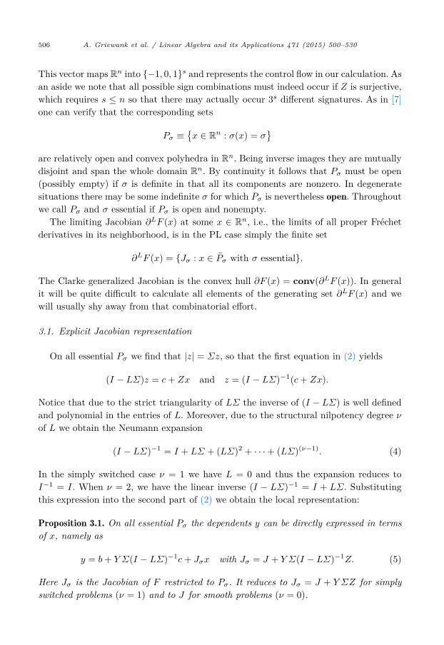
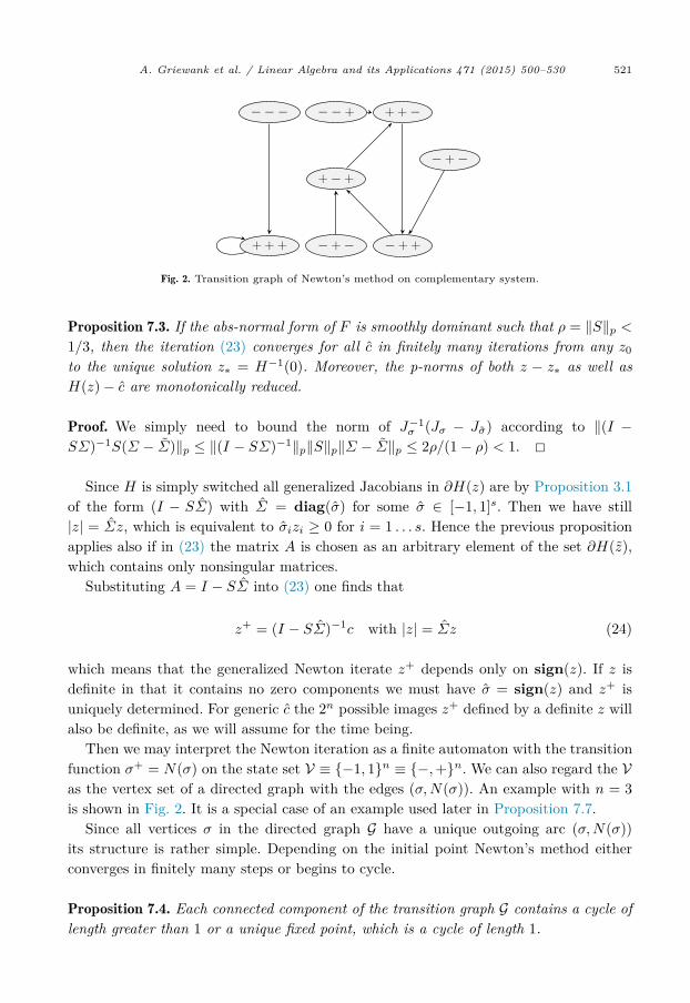
Fig. 2. Transition graph of Newton’s method on complementary system.

Proposition 7.3. If the abs-normal form of F is smoothly dominant such that ρ = ‖S‖p <

1/3, then the iteration (23) converges for all c in finitely many iterations from any z0

to the unique solution z∗ = H−1(0). Moreover, the p-norms of both z − z∗ as well as H(z) − c are monotonically reduced.

Proof. We simply need to bound the norm of J−1σ (Jσ − Jσ) according to ‖(I −

SΣ)−1S(Σ − Σ)‖p ≤ ‖(I − SΣ)−1‖p‖S‖p‖Σ − Σ‖p ≤ 2ρ/(1 − ρ) < 1. �Since H is simply switched all generalized Jacobians in ∂H(z) are by Proposition 3.1

of the form (I − SΣ) with Σ = diag(σ) for some σ ∈ [−1, 1]s. Then we have still |z| = Σz, which is equivalent to σizi ≥ 0 for i = 1 . . . s. Hence the previous proposition applies also if in (23) the matrix A is chosen as an arbitrary element of the set ∂H(z), which contains only nonsingular matrices.

Substituting A = I − SΣ into (23) one finds that

z+ = (I − SΣ)−1c with |z| = Σz (24)

which means that the generalized Newton iterate z+ depends only on sign(z). If z is definite in that it contains no zero components we must have σ = sign(z) and z+ is uniquely determined. For generic c the 2n possible images z+ defined by a definite z will also be definite, as we will assume for the time being.

Then we may interpret the Newton iteration as a finite automaton with the transition function σ+ = N(σ) on the state set V ≡ {−1, 1}n ≡ {−, +}n. We can also regard the Vas the vertex set of a directed graph with the edges (σ, N(σ)). An example with n = 3is shown in Fig. 2. It is a special case of an example used later in Proposition 7.7.

Since all vertices σ in the directed graph G have a unique outgoing arc (σ, N(σ))its structure is rather simple. Depending on the initial point Newton’s method either converges in finitely many steps or begins to cycle.

Proposition 7.4. Each connected component of the transition graph G contains a cycle of length greater than 1 or a unique fixed point, which is a cycle of length 1.

522 A. Griewank et al. / Linear Algebra and its Applications 471 (2015) 500–530

Proof. From any initial σ0 the sequence of iterations σk = Nk(σ0) stays in the connected component of σ0 and must reach a fixed point or begin to cycle. Let C(σ0) denote the set of vertices that are touched infinitely often by this sequence. Let Prec(C(σ0)) denote the set of all σ ∈ G with C(σ) = C(σ0). We now have to exclude that the connected subgraph Prec(C(σ0)) has outgoing or incoming edges. There can be no incoming edges because repeatedly applying N to their origins would also lead to C(σ0). Also there can be no outgoing edges because their origins would lead to a cycle or fixed point outside Prec(C(σ0)). This completes the proof. �

While the condition ρ = ‖S‖p < 1/3 used in Proposition 7.3 excludes cycling it does seem rather strong. Alternatively, we may impose the condition ρ(|S|) < 1/2, which allows us to prove finite termination and even limit the computational effort to n3/3fused multiply adds.

Proposition 7.5. Let the Schur complement |S| be absolutely contractive with ρ = ρ(|S|) <1/2 or ρ = 1/2 and S irreducible. Then for all c any iteration (24) converges in at most s iterations from any z0 to the unique solution z∗ = H−1(c).

Proof. After equilibration by the Perron–Frobenius vector we may assume without loss of generality that ρ = ρ(|S|) = ‖S‖∞ ≤ 1/2. For notational simplicity we drop the superscript ˆ and write σ ∈ [−1, 1]s and Σ = diag(σ) with the only restriction that at the current iterate z we have |z| = Σz.

The argument below will be based on the fact that for ‖S‖∞ ≤ 1/2 with S irreducible, the inverse (I − SΣ)−1 is strictly diagonally dominant with a positive diagonal. We will prove this statement for ‖S‖∞ < 1/2. The limiting case requires a more extensive reasoning, for which we refer to Lemma 4.2 in [20].

Since ‖SΣ‖∞ ≤ ‖S‖∞‖Σ‖∞ ≤ ‖S‖∞ it suffices to consider the case Σ = I: We have ‖Sk‖∞ ≤ ‖S‖k∞ < 1

2k which implies limk→∞ Sk = 0. Hence we can express (I − S)−1

via the Neumann series

A−1 =∞∑k=0

(I −A)k =∞∑k=0

Sk = I +∞∑k=1

Sk.

The inequality ‖ ∑∞

k=1 Sk‖∞ ≤

∑∞k=1 ‖S‖k∞ <

∑∞k=1

12k = 1 already ensures strict

diagonal dominance for (I − S)−1.Now we perform symmetric pivoting by reordering the equations and the components

of z such that the first component c1 of the permuted vector c is its largest, i.e., |c1| =‖c‖∞. Note that reorderings of the equations and variables do not affect the generalized Newton iteration at all. If c1 = 0 we must have that c = 0 and thus z+ = 0 is obtained as the correct solution from any z in one step. Otherwise we have for the first component of the defining equation

∣∣z+1 − c1

∣∣ =∣∣e�1 SΣz+∣∣ ≤ ‖e1S‖1

∥∥z+∥∥ ≤ ρ2|c1| < |c1|.

∞

A. Griewank et al. / Linear Algebra and its Applications 471 (2015) 500–530 523

This ensures that the sign of the first component z+1 is the same as that of σ∗

1 ≡sign(c1) = 0 and we have the crucial identity |z+

1 | = σ∗1z

+1 . This will remain true over

all subsequent iterations since we have so far not imposed any assumptions on the step defining σ whatsoever. Hence we may assume that from the second iteration onwards already σ1 = σ∗

1 and thus also |z+1 | = σ1z

+1 . This relation allows us to rewrite the first

equation and express it as a linear combination of the other z+j , namely

z+1(1 − σ∗

1s11)

= c1 +s∑

j=2s1jσjz

+j =⇒ σ1z

+1 = c1

σ∗1 − s11

+s∑

j=2

s1jσjz+j

σ∗1 − s11

.

Substituting this relation into the other equations, which corresponds to one step of Gaussian elimination, we obtain for i = 2 . . . s

z+i = ci + si1c1

σ∗1 − s11

+s∑

j=2

[sij + si1s1j

σ∗1 − s11

]σjz

+j ≡ ci +

s∑j=2

sijσjz+j .

Hence we see that the other components z+i for i = 2 . . . s are equivalent to the ones that

would be obtained on the reduced system with the same restriction for picking σi, namely σizi = |zi|. The implicitly reduced matrix S ≡ (sij)i=2...s

j=2...s satisfies ‖S‖∞ ≤ ρ = ‖S‖∞since, for each i > 1,

s∑j=2

|sij | ≤s∑

j=2|sij | +

|si1|1 − σ∗

1s11

s∑j=2

|s1j | ≤ ρ− |si1| +|si1|(ρ− |s11|)

1 − σ∗1s11

≤ ρ− |si1|2 ≤ ρ.

Thus we can repeat the argument and after the second iteration the sign of the z+i

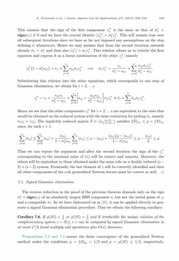
corresponding to the maximal value of |ci| will be correct and nonzero. Moreover, the others will be equivalent to those obtained under the same rule on a doubly reduced (s −2) × (s − 2) system. Eventually the last element of z will be correctly identified and then all other components of the s-th generalized Newton iterate must be correct as well. �7.3. Signed Gaussian elimination

The system reduction in the proof of the previous theorem depends only on the sign σ∗i = sign(ci) of an absolutely largest RHS component ci but not the initial guess of zi

and a compatible σi. As we have elaborated on in [20], it can be applied directly to gen-erate a signed Gaussian elimination procedure. Thus we obtain the following corollary:

Corollary 7.6. If ρ(|S|) < 12 or ρ(|S|) = 1

2 and S irreducible the unique solution of the complementary system z = S|z| + c can be computed by signed Gaussian elimination in at most s3/3 fused multiply add operations plus O(s) divisions.

Propositions 7.3 and 7.5 ensure the finite convergence of the generalized Newton method under the conditions ρ = ‖S‖p < 1/3 and ρ = ρ(|S|) ≤ 1/2, respectively.

524 A. Griewank et al. / Linear Algebra and its Applications 471 (2015) 500–530

Obviously, the second condition does not imply the former, but the converse does also not hold so that there are problems where only one but not both theorems apply. To demonstrate this we consider the example

S = 0.3[I − ee�/9

]∈ R

9 with e = (1)1...9.

Here S is a scaled elementary reflector so that ρ = ‖S‖2 = 0.3 · 1 < 1/3. However, one can easily check that ρ(|S|) = 0.3 · 16/9 = 1.6/3 > 0.5 so that Proposition 7.3 applies, but neither Proposition 7.5 nor its Corollary 7.6.

7.4. Divergence of the generalized Newton on cyclic example

Another question that arises is whether the bound 1/2 imposed on ρ = ρ(|S|) in Proposition 7.5 and its corollary could not be weakened. The answer is that for s of any significant size the bound may only be raised a minute amount above 1/2 without opening the possibility of divergence. More specifically, we have the following family of counter examples, whose instance for s = 3 was already depicted in Fig. 2.

Proposition 7.7. For s > 2 set c = (1)1...s and define S ∈ Rs×s as the cyclic Töplitz

matrix

S =[

0 a

aIs−1 0

].

Then, if a ∈ R satisfies

12 + 1

2s ≤ a ≤ 1√2,

the generalized Newton method cycles between s distinct and definite points when the initial z contains exactly one negative component and no zeros.

Proof. Suppose the current approximation z = (zi)si=1 consists of only positive compo-nents except for one, say zi < 0. Then we will show that the next iterate z+ has only positive iterates except for 0 > z+

i+ with i+ ≡ 1 + (i mod s). This relation obviously establishes the assertion, since the single negative sign will cycle infinitely often. Due to the symmetry of the situation we may assume w.l.o.g. that the last component of the current iterate z is negative. Hence here we have Σ(z) = diag(1, . . . , 1, −1) and the next iterate ζ = z+ is then the solution of the system of linear equations,

⎡⎢⎢⎢⎣

1 0 . . . a

−a 1 . . . 0. . .

⎤⎥⎥⎥⎦

⎡⎢⎢⎢⎣ζ1...

⎤⎥⎥⎥⎦ =

⎡⎢⎢⎣

1...

⎤⎥⎥⎦

−a 1 ζs 1

A. Griewank et al. / Linear Algebra and its Applications 471 (2015) 500–530 525

Thus in terms of ζ1 the other components ζi for i = 2, . . . , s are given by

ζi = 1 + aζi−1 =(

1 − ai−1

1 − a

)+ ai−1ζ1

Substituting these expressions into the first line of the system we find

ζ1 + aζs = 1 =⇒ ζ1 + a(1 − as−1)

(1 − a) + asζ1 = 1 =⇒ ζ1 = 1 − 2a + as

(1 + as)(1 − a) .

Now we want to achieve a shift of the negative entry from the last to the first position during the iteration from z to z+. So ζ1 should become negative and ζ2 has to stay positive. In other words, we have to impose the two conditions ζ1 < 0 and ζ2 > 0. From the first one it follows that

0 > 1 − a(1 − as−1)

(1 − a) ⇐⇒s−1∑i=0

ai > 2

and the second one is equivalent to

0 < ζ2 = 1 + aζ1 = 1 + a

(1 + as)

[1 − a

(1 − as−1)(1 − a)

]⇐⇒ 1 + as > 2a2.

The last condition is certainly met by all a ≤ 1/√

2 < 1. To ensure the first condition ζ1 < 0 we substitute a = 1

2(1 + Δa) for some Δa ∈ (0, √

2 − 1). Clearly, the first condition is monotonic in a and Δa so that, if it holds for the particular Δa = 21−s, it must also hold for all greater values of that problem parameter. Now we obtain after some elementary manipulations

s−1∑i=0

[12(1 + Δa)

]i> 2 ⇐⇒

1 − [ 12 (1 + Δa)]s

1 − 12 (1 + Δa)

> 2 ⇐⇒ Δa < 2 s√

Δa− 1.

The only thing that remains to be shown is that the last inequality holds for Δa ≡ 21−s. For s = 3 this is easily verified by direct calculation. For all s ≥ 4 we obtain the condition

2 s√

Δa− 1 = 21/s − 1 ≥ 1/(2s).

Here, the last inequality holds for s ≥ 2 since the function 21/s − 1 − 1/(2s) of s is positive for s = 2 and one can easily check by differentiation that it grows monotonically beyond. Now all that remains to be shown is that 2s−2 < 1/s, which one can check quite easily to be indeed satisfied for all s > 3. This completes the proof. �

526 A. Griewank et al. / Linear Algebra and its Applications 471 (2015) 500–530

The proposition demonstrates that, at least without additional structural informa-tion on S, we cannot deduce the convergence of full step generalized Newton when ρ(|S|) ∈ [1/2 + 1/2n,

√2]. Also, because our fixed point iteration and the modulus

method normally yield only linear convergence, it becomes immediately clear that they do not reduce to semi-smooth Newton. Under the assumption of smooth dominance the local convergence result of Qi et al. applies and we must have finite convergence on PL problems whenever convergence occurs at all. Of course, evaluating H(z) is a lot cheaper than solving a system in the Jacobian Jσ = J + Y Σ(I − LΣ)−1Z with σ = σ(x) and thus Σ = Σ(x), changing from iterate to iterate. While the iteration function G is Lipschitzian, the not always unique generalized Newton steps −J−1

σ(x)F (x)may jump discontinuously as a function of x. Nevertheless, it might be worthwhile to switch to Newton once the signature vector σ has been stable for a few itera-tions.

It is not too hard to see that (at least when full steps are taken) the general-ized Newton iteration on H(z) is equivalent to that applied to the partitioned equa-tion (2) for fixed y. The key numerical effort is solving a linear system in I − SΣ, which is also the key effort in applying the inverse Jacobians J−1

σ to any vector. In either case we first need to form the Schur complement S, which, at least for-mally, involves the inverse of the smooth part J . If the number s of switching vari-ables is much smaller than n, the number of independents, we can of course compute J−1Y or ZJ−1 by solving s linear systems in J , possibly based on its LU factoriza-tion.

When H(z) is injective, the fibers (15) have no bifurcations at all, so trac-ing them in a piecewise Newton fashion seems a very promising approach. Nat-urally, the number of steps is not a priori bounded below the exponential num-ber 2s of orthants in Rs. The same is true for the sign accord method that was first introduced by Rohn in [21] and further investigated by the latter in [22], as well as by Neumaier in [16]. The sign accord algorithm is also finitely con-vergent under the equivalent condition of S being partially contractive. The two methods are quite different, since piecewise Newton strongly depends on the ini-tial point but not on the ordering of the variables and equations, whereas the sign accord algorithm depends only on the initial orthant but is effected by reorder-ings.

To see that piecewise Newton is not equivalent to applying piecewise Newton to the original system F (x) = 0 we note that in the latter case, until the final step, there will always be a nontrivial residual on the lower equation of (2), whereas the upper block will be exactly satisfied. Conversely, applying piecewise Newton to H(z) = c means that there will be a residual in the upper block but the lower equa-tion will remain exactly satisfied. Of course, one could also try a mixture just start-ing from (x, z) = (0, 0) so that all subsequent residuals would be multiples of (c, b). The advantages and disadvantaged of these approaches deserve to be explored in de-tail.

A. Griewank et al. / Linear Algebra and its Applications 471 (2015) 500–530 527

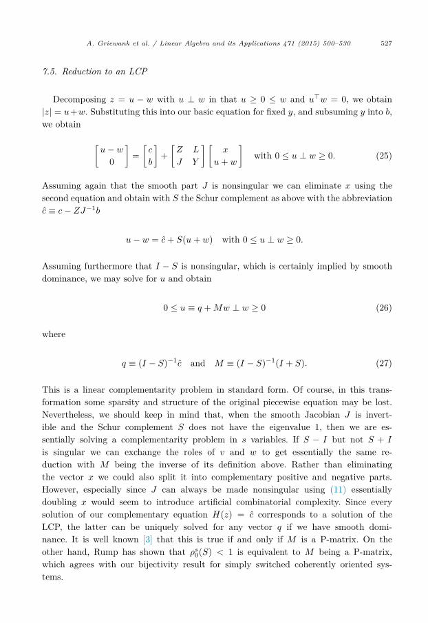
7.5. Reduction to an LCP

Decomposing z = u − w with u ⊥ w in that u ≥ 0 ≤ w and u�w = 0, we obtain |z| = u +w. Substituting this into our basic equation for fixed y, and subsuming y into b, we obtain

[u− w

0

]=

[c

b

]+

[Z L

J Y

] [x

u + w

]with 0 ≤ u ⊥ w ≥ 0. (25)

Assuming again that the smooth part J is nonsingular we can eliminate x using the second equation and obtain with S the Schur complement as above with the abbreviation c ≡ c − ZJ−1b

u− w = c + S(u + w) with 0 ≤ u ⊥ w ≥ 0.

Assuming furthermore that I − S is nonsingular, which is certainly implied by smooth dominance, we may solve for u and obtain

0 ≤ u ≡ q + Mw ⊥ w ≥ 0 (26)

where

q ≡ (I − S)−1c and M ≡ (I − S)−1(I + S). (27)

This is a linear complementarity problem in standard form. Of course, in this trans-formation some sparsity and structure of the original piecewise equation may be lost. Nevertheless, we should keep in mind that, when the smooth Jacobian J is invert-ible and the Schur complement S does not have the eigenvalue 1, then we are es-sentially solving a complementarity problem in s variables. If S − I but not S + I

is singular we can exchange the roles of v and w to get essentially the same re-duction with M being the inverse of its definition above. Rather than eliminating the vector x we could also split it into complementary positive and negative parts. However, especially since J can always be made nonsingular using (11) essentially doubling x would seem to introduce artificial combinatorial complexity. Since every solution of our complementary equation H(z) = c corresponds to a solution of the LCP, the latter can be uniquely solved for any vector q if we have smooth domi-nance. It is well known [3] that this is true if and only if M is a P-matrix. On the other hand, Rump has shown that ρs0(S) < 1 is equivalent to M being a P-matrix, which agrees with our bijectivity result for simply switched coherently oriented sys-tems.

528 A. Griewank et al. / Linear Algebra and its Applications 471 (2015) 500–530

8. Summary and outlook

In this paper we have examined the properties of piecewise linear functions that are given in abs-normal form. Such a representation is always possible, but by no means unique. A key quantity is the switching depth ν, which we conjecture to be reducible to the bound ν(n) = 2n − 1. Of particular importance is the case of ν = 1, where we call F simply switched. If such a representation exists, it is shown here that openness and bijectivity coincide provided LIKQ or the slightly weaker nondegeneracy condition of stable coherent orientation is satisfied.

The Schur complement matrix S = L − ZJ−1Y , whose existence depends on the nonsingularity of the smooth part J , plays a central role throughout. In particular it yields the complementary system H(z) = [I − SΣ]z = c. This piecewise linear func-tion H(z) is simply switched and satisfies the LIKQ condition. Hence it is, according to Proposition 4.1, injective if and only if it is coherently oriented, which, in turn, is equivalent to the signed real spectral radius of S being less than 1. In principle this can be tested, though the evaluation of the continuous function ρs0(S) is generally NP hard as shown in [23]. Since injectivity of H(z) implies injectivity of the underlying F (x) the partial contractivity condition ρs0(S) < 1 is also sufficient for injectivity of F (x). How-ever, we have as yet no practical criterion for F (x) to be merely open other than the theoretical possibility of exhaustively checking all Jacobians of F . Such combinatorial procedures have otherwise been avoidable throughout, thanks to the representation of Fin abs-normal form. The key properties form the following chain of implications:

Absolute Contractivity =⇒ Smooth Dominance =⇒ Bijectivity of H

ρ(|S|

)< 1

∥∥DSD−1∥∥p< 1 ρs0(S) < 1.

So far our Linear Independence Kink Qualification (LIKQ) has only been defined in the simply switched case and it is then equivalent to the familiar linear independence constraint qualification (LICQ). However, there is a generalization to PL problems, where the kinks do not even locally consist of a set of intersecting hyperplanes, as is often envisioned. Instead, there is a hierarchy of kinks with later ones being broken into affine pieces by earlier ones. The algorithmic handling of this structure is not yet clear.

In order to constructively solve PL systems of equations one may apply full-step or piecewise Newton to either the original problem F (x) = 0 or the complementary version H(z) = c. They are guaranteed to converge if S does not deviate too much from L, which ensures at least coherent orientation. More specifically, we obtain finite convergence of generalized Newton on H(z) = c when ‖S‖p < 1/3 or ρ(|S|) < 1/2. The second bound is quite sharp in that divergence can occur as soon as ρ(|S|) ≥ 1/2 +1/2n, as demonstrated in Proposition 7.7. Apart from these four variants one may apply damped versions or the fixed point iteration z+ = c + S|z|, provided one has smooth dominance, i.e., ‖S‖p < 1for some p ≥ 1, which is stronger than coherent orientation of H and thus injectivity of F , H.

A. Griewank et al. / Linear Algebra and its Applications 471 (2015) 500–530 529

Piecewise smooth problems can be solved by successive piecewise linearization, yield-ing at least locally quadratic convergence. In this context coherent orientation of the piecewise linear model near the current outer iterate should be sufficient. Abbreviating ρ = ‖J−1Y ‖p‖Z‖p we may compile the table of solvers listed in Table 1. The effort column shows, which linear systems need to be solved, usually once per iteration. In the signed Gaussian elimination the equivalent of just one single solve is needed.

Table 1Solvers for PL systems of equations in original abs-normal or complementary form.

Method Convergence condition Rate Effort

Generalized Newton on OPL 2ρ < (1 − ‖L‖p − ρ/2)2 finite I − SΣ, JGeneralized Newton on CPL ‖S‖p < 1/3 finite I − SΣSigned Gauss on CPL ρ(|S|) < 1/2 finite I − SΣ onceBlock Seidel on CPL ‖S − L‖p + ‖L‖p < 1 linear I − LΣ, JModulus iteration on CPL ‖S‖p < 1 linear JPiecewise Newton on OPL coherent orientation of F finite I − SΣ, JPiecewise Newton on CPL partial contractivity of S finite I − SΣ

Another theoretical possibility is piecewise Newton on the combined system in terms of x and z. A more promising approach would appear to be the combination of the fixed point iterations with Newton variants, which should yield finite convergence if one can get into the vicinity of a root. Without coherent orientation the fibers {F (x) = λF (x0) :λ > 0} and also {H(z) − c = λ(H(z0) − c) : λ > 0} may contain turning points, which could be followed by some version of Branin’s method [2] originally defined by

x = ±adj(F ′(x)

)F (x) with det

(F ′(x)

)I = F ′(x)adj

(F ′(x)

).

In the general smooth case such trajectories may converge to roots, cycle or run off to infinity. Possibly the inherent finiteness of PL functions makes it possible to avoid some of these calamities. Other globalized searches remain to be investigated. Since any Lipschitzian vector function may be approximated on compact domains by PL functions, there can be no magic solver for the general case. Numerical experiments with the various methods considered here are currently under way.

Acknowledgements

The proof of Lemma 4.3 and Proposition 4.4 was thankfully provided by our colleague Dorothee Schüth of Humboldt University. The authors are also indebted to Daniel Kress-ner, who pointed out the connection between the coherence condition det(I −ΣS) > 0and the sign real spectral radius ρs0(S) of the Schur complement S being less than 1. They are also grateful to Torsten Bosse, who contributed many insights into the piecewise lin-earization approach and greatly helped with the composition of this article. Finally, the paper benefited greatly from the corrections and suggestions – most notable: the pointer to the fundamental contributions of J. Rohn – by the two anonymous referees.

530 A. Griewank et al. / Linear Algebra and its Applications 471 (2015) 500–530

References

[1] Luigi Brugnano, Vincenzo Casulli, Iterative solution of piecewise linear systems, SIAM J. Sci. Com-put. 30 (1) (2008) 463–472.

[2] Franklin H. Branin, Widely convergent method for finding multiple solutions of simultaneous non-linear equations, IBM J. Res. Develop. 16 (5) (1972) 504–522.

[3] Richard W. Cottle, Jong-Shi Pang, Richard E. Stone, The Linear Complementarity Problem, Com-pututer Science and Scientific Computing, Academic Press, Inc., Boston, MA, 1992, 762 p.

[4] Iain S. Duff, Albert Maurice Erisman, John Ker Reid, Direct Methods for Sparse Matrices, Claren-don Press, Oxford, 1986.

[5] Francisco Facchinei, Jong-Shi Pang, Finite-Dimensional Variational Inequalities and Complemen-tarity Problems, vol. 1, Springer, 2003.

[6] Björn Geißler, Alexander Martin, Antonio Morsi, Lars Schewe, Using piecewise linear functions for solving MINLPs, in: Jon Lee, Sven Leyffer (Eds.), Mixed Integer Nonlinear Programming, in: IMA Vol. Math. Appl., vol. 154, Springer, New York, 2012, pp. 287–314.

[7] Andreas Griewank, On stable piecewise linearization and generalized algorithmic differentiation, Optim. Methods Softw. 28 (6) (2013) 1139–1178.

[8] M. Golubitsky, D.G. Schaeffer, Singularities and Groups in Bifurcation Theory, vol. 1, Springer, New York, 1985.

[9] Andreas Griewank, Andrea Walther, Evaluating Derivatives: Principles and Techniques of Algorith-mic Differentiation, SIAM, 2008.

[10] A. Hadjidimos, M. Lapidakis, M. Tzoumas, On iterative solution for linear complementarity problem with an h+-matrix, SIAM J. Matrix Anal. Appl. 33 (1) (2012) 97–110.

[11] Kamil A. Khan, Paul I. Barton, Evaluating an element of the Clarke generalized Jacobian of a piecewise differentiable function, in: Recent Advances in Algorithmic Differentiation, in: Lect. Notes Comput. Sci. Eng., vol. 87, Springer, Berlin, Heidelberg, 2012, pp. 115–125.

[12] Kamil A. Khan, Paul I. Barton, Evaluating an element of the Clarke generalized Jacobian of a composite piecewise differentiable function, ACM Trans. Math. Software (TOMS) 39 (4) (July 2013) 23:1–23:28.

[13] Tom A.M. Kevenaar, Domine M.W. Leenaerts, A comparison of piecewise-linear model descriptions, IEEE Trans. Circuits Syst. I, Fundam. Theory Appl. 39 (12) (1992) 996–1004.

[14] O.L. Mangasarian, R.R. Meyer, Absolute value equations, Linear Algebra Appl. 419 (2) (2006) 359–367.

[15] Yurii Nesterov, Lexicographic differentiation of nonsmooth functions, Math. Program. 104 (2–3) (2005) 669–700.

[16] A. Neumaier, Interval Methods for Systems of Equations, Cambridge University Press, 1990.[17] Julia Piontkowski, Andreas Griewank, Solution of complementarity problems via piecewise lineariza-

tion, PAMM 13 (1) (2013) 581–584.[18] L. Qi, J. Sun, A nonsmooth version of Newton’s method, Math. Program. 58 (3) (1993) 353–368.[19] A. Quarteroni, R. Sacco, F. Saleri, Numerical, Texts Appl. Math., Springer-Verlag GmbH, Berlin,

2000.[20] M. Radons, Direct solution of piecewise linear systems, in preparation.[21] Jiri Rohn, Systems of linear interval equations, Linear Algebra Appl. 126 (1989) 39–78.[22] Jiri Rohn, An algorithm for solving the absolute value equation, Electron. J. Linear Algebra

18 (589–599) (2009) 5.[23] Siegfried M. Rump, Theorems of Perron–Frobenius type for matrices without sign restrictions,

Linear Algebra Appl. 266 (1997) 1–42.[24] M. Ruzicka, Nichtlineare Funktionalanalysis. Eine Einführung, Springer, Berlin, 2004.[25] Stefan Scholtes, Introduction to Piecewise Differentiable Equations, Springer, 2012.[26] Thomas Edwin Stern, Piecewise-linear network theory, Tech. Rep. 315, Research Laboratory of

Electronics, Massachusetts Institute of Technology, Cambridge, MA, 1956.[27] Wilhelmus Maria Gezinus van Bokhoven, Piecewise-Linear Modelling and Analysis, Kluwer Tech-

nische Boeken, 1981.[28] Wim M.G. Van Bokhoven, Domine M.W. Leenaerts, Explicit formulas for the solutions of piecewise

linear networks, IEEE Trans. Circuits Syst. I, Fundam. Theory Appl. 46 (9) (1999) 1110–1117.