Linear Algebra in Actuarial Science: Slides to the lecture · PDF fileLinear Equation...

Linear Equation Systems Vector Spaces Eigenvalues and Eigenvectors Numerical Issues

Linear Algebra in Actuarial Science:Slides to the lecture

Fall Semester 2010/2011

Linear Algebra in Actuarial Science: Slides to the lecture


Linear Algebra is a Tool-BoxLinear Equation SystemsDiscretization of differential equations: solving linear equationssystems

1 α 0 0 0 . . . 0−α 1 α 0 0 . . . 00 −α 1 α 0 . . . 0...

...0 0 0 . . . 0 −α 1

=

V (0)0...0

V (n)

I Existence of solution ?I Uniqueness of solution ?I Stability of solution ?



Linear Algebra is a Tool-Box

Minimization ProblemI Given data vector b and parameter matrix A.I Find x such that ||Ax − b|| gets minimal.

Idea: Suitable transform of parameters and dataSolution: Decomposition of matrices




Bonus-Malus-SystemsCar insurance with two different premium-levels a < c .

I Claim in the last year or in the year before: premium cI No claims in the last two years: premium a.I P(Claim in one year) = p = 1− q,

P =

p q 0p 0 qp 0 q

Question: What is right choice for a and c ?Markov Chains with stationary distributions: What is limn→∞ Pn ?




Construction of index-linked products with n underlyings

I Classical models use normal distribution assumptions for assetsI Basket leads to multivariate normal distributionI What is the square root of a matrix ?I How can simulations be done on covariance matrices ?

Idea: Transform the matrixSolution: Decomposition of matrices



Linear Algebra

Syllabus

Linear Equation Systems: Gauss Algorithm, Existence andUniqueness of Solutions, Inverse, Determinants

Vector Spaces: Linear (In-)Dependence, Basis, Inner Products,Gram-Schmidt Algorithm

Eigenvalues and Eigenvectors: Determination, Diagonalisation,Singular Values

Decompositions of Matrices: LU, SVD, QR, Cholesky



Field Axioms

DefinitionA field is a set F with two operations, called addition andmultiplication, which satisfy the following so-called "field axioms"(A), (M) and (D):(A) Axioms for addition

(A1) If x ∈ F and y ∈ F , then x + y ∈ F .(A2) Addition is commutative: x + y = y + x for all x , y ∈ F .(A3) Addition is associative: (x + y) + z = x + (y + z) for all

x , y , z ∈ F .(A4) F contains an element 0 such that 0 + x = x for all x ∈ F .(A5) To every x ∈ F corresponds an element −x ∈ F such that

x + (−x) = 0.



Field Axioms

DefinitionField definition continued:

(M) Axioms for multiplication(M1) If x ∈ F and y ∈ F , then xy ∈ F .(M2) Multiplication is commutative: xy = yx for all x , y ∈ F .(M3) Multiplication is associative: (xy)z = x(yz) for all x , y , z ∈ F .(M4) F contains an element 1 6= 0 such that 1x = x for all x ∈ F .(M5) If x ∈ F and x 6= 0 then exists an element 1/x ∈ F such that

x · (1/x) = 1.

(D) The distributive law x(y + z) = xy + xz holds for allx , y , z ∈ F .



Addition of Matrices

(A1) A = B ⇔ aij = bij , ∀1 ≤ i ≤ m, 1 ≤ j ≤ n.(A2) A ∈ M(m × n),B ∈ M(m × n) ⇒ A + B := (aij + bij).(A3) Addition is commutative: A + B = B + A.(A4) Addition is associative: (A + B) + C = A + (B + C ).

(A5) Identity element: A =

0 . . . 0...

. . ....

0 . . . 0

.

(A6) Negative element: −A = −(aij).



Multiplication of Matrices

(M1) A ∈ M(m×n),B ∈ M(n×r)⇒ C = A·B = (cik) ∈ M(m×r),

cik = ai1b1k + . . .+ ainbnk =n∑

j=1

aijbjk .

(M2) Multiplication of matrices is in general not commutative !(M3) Multiplication of matrices is associative.

(M4) Identity matrix: I = In =

1 . . . 0...

. . ....

0 . . . 1

∈ M(n × n).

(M5) A · I = I · A, but A · B = A · C does not imply in generalB = C !



Transpose, Inverse, Multiplication with scalars

(M) Transpose and Inverse(T) Transpose of A: AT , with

(AT )T = A, (A + B)T = AT + BT and (A · B)T = BT · AT .

(I) Given A ∈ M(n × n) and X ∈ M(n × n). If A · X = X · A = I ,then X = A−1 is the inverse of A.

(Ms) Multiplication with scalars(Ms1) λ ∈ K,A ∈ M(m × n) ⇒ λA := (λaij).(Ms2) Multiplication with scalars is commutative and associative.(Ms3) The distributive law holds: (λ+ µ)A = λA + µA.



The inverse of a matrix

TheoremIf A−1 exists, it is unique.

DefinitionA ∈ M(n × n) is called singular, if A−1 does not exist. Otherwise itis called non-singular.

TheoremGiven A,B ∈ M(n × n) non-singular. Then it follows

I A · B non-singular and (A · B)−1 = B−1 · A−1.

I A−1 non-singular and (A−1)−1 = A.I AT non-singular and (AT )−1 = (A−1)T .



Gauss-Algorithm

Example

2u + v + w = 14u + v = −2−2u + 2v + w = 7

⇒ Gauss-Algorithm ⇒

2u + v + w = 1− 1v − 2w = −4

− 4w = −4



Theorems: Solutions under Gauss-Algorithm

TheoremGiven a matrix A ∈ M(m × n)

1. The Gauss-Algorithm transforms in a finite number of steps Ainto an upper triangular matrix A′.

2. rank(A) = rank(A′).3. Given the augmented matrix (A, b) and the upper triangular

matrix (A′, b′). Then x is a solution of Ax = b ⇔ x is asolution of A′x = b′.



Theorems: Solutions under Gauss-Algorithm

TheoremGiven

A ∈ M(m × n), b =

b1...bm

∈ Rm, x =

x1...xn

∈ Rn.

The linear equation system Ax = b has a solution, ifrank(A)=rank(A, b).The linear equation system has a unique solution, ifrank(A)=rank(A, b)=n.



Theorems: Solutions under Gauss-AlgorithmTheoremGiven x0 a particulate solution of Ax = b. Then the solutions x ofAx = b have the form x = x0 + h, where h is the general solutionof the homogeneous equation system.

Corollary

1. Ax = b has an unique solution ⇔{Ax = b has a solution.Ax = 0, has only the solution x = 0.

2. A ∈ M(n × n):Ax = b has an unique solution ⇔ rank(A) = n ⇔ A isnon-singular ⇔ Ax = 0 has only the solution x = 0.The solution of Ax = b is given as x = A−1b.

3. rank(A) = n ⇔ A−1 exists.Linear Algebra in Actuarial Science: Slides to the lecture


Determination of DeterminantsA ∈ M(2× 2, R)

A =

(a11 a12a21 a22

)⇒ det(A) = a11 · a22 − a12 · a21

A ∈ M(3× 3, R): Rule of Sarrus

A =

a11 a12 a13a21 a22 a23a31 a32 a33

⇒∣∣∣∣∣∣a11 a12 a13a21 a22 a23a31 a32 a33

∣∣∣∣∣∣a11 a12a21 a22a31 a32

⇒ det(A) = a11 · a22 · a33 + a12 · a23 · a31 + a13 · a21 · a32

− a13 · a22 · a31 − a11 · a23 · a32 − a12 · a21 · a33



Determination of DeterminantsA ∈ M(n × n, R)

DefinitionGiven a matrix A = (aij) ∈ M(n × n). The minor A′ij is thedeterminant of the matrix ∈ M(n − 1× n − 1) obtained byremoving the i-th row and the j-th column of A. The associatedcofactor Cij = (−1)i+jA′ij .

DefinitionThe determinant of a matrix A = (aij) ∈ M(n × n) is defined by

det(A) =n∑

j=1

(−1)1+ja1jA′1j =n∑

j=1

a1jC1j ,

i.e. Laplace expansion with first row.Linear Algebra in Actuarial Science: Slides to the lecture


Determinants: Properties1. det(AT ) = det(A)

2. ∃i : ai = (0, . . . , 0)⇒ det(A) = 03. det(λA) = λndet(A), if A ∈ M(n × n)

4. ∃i , j : i 6= j and ai = aj ⇒ det(A) = 05. (1) det(A · B) = detA · detB

(2) det(A + B) 6= det(A) + det(B)

6. A ↪→ A′ through changing of n rows ⇒ det(A′) = (−1)ndet(A)

7. A ↪→ A′ through multiplication of i-th row with λ⇒ det(A′) = λdet(A)

8. A ↪→ A′ through adding the λ-fold of i-th row to the j-th row⇒ det(A′) = det(A)

9. A is non-singular ⇔ rank(A) = n ⇔ det(A) 6= 0 ⇔det(A−1) = 1

det(A)

10. If A = diag(a11, . . . , ann)⇒ det(A) =∏n

k=1 akk



General vector spacesDefinitionGiven K some field. A non-empty set V is called a K-vector space,if

I for all a, b ∈ V ⇒ a + b ∈ V .I for all λ ∈ K and a ∈ V ⇒ λ · a ∈ V .

The field is closed with respect to addition and multiplication withscalars.

DefinitionGiven V a K-vector space. A non-empty subset U ⊂ V is called alinear subspace of V if for all λ ∈ K and a, b ∈ U

a + b ∈ U, λ · a ∈ U.



Linear combination and span(U)

DefinitionGiven scalars λ1, . . . , λm ∈ K and vectors a1, . . . , am ∈ V . A vectora = λ1a1 + . . .+ λmam is called a linear combination of a1, . . . , am.The linear combination is called trivial, if λ1 = . . . = λm = 0,otherwise it is called non-trivial.

DefinitionGiven U ⊂ V a non-empty subset. The set of all linearcombinations of vectors in U

span(U) ={a =

∑λiai , λi ∈ K, ai ∈ U

}is called span(U).



Linear independencyDefinitionThe vectors a1, . . . , am ∈ V are called linearly dependent (l.d.), if thereexists a non-trivial linear combination, such that

λ1a1 + . . .+ λmam = 0, ∃i : λi 6= 0.

The vectors a1, . . . , am ∈ V are called linearly independent (l.i.), if theyare not linearly dependent.

TheoremGiven vectors a1, . . . , am ∈ V . The following is equivalent:

1. The vectors a1, . . . , am are linearly dependent.

2. At least one vector ai is a linear combination of the other, i.e.

∃i ∈ {1, . . . ,m} : ai =∑j 6=i

λjaj .



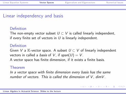
Linear independency and basis

DefinitionThe non-empty vector subset U ⊂ V is called linearly independent,if every finite set of vectors in U is linearly independent.

DefinitionGiven V a K-vector space. A subset U ⊂ V of linearly independentvectors in called a basis of V , if span(U) = V .A vector space has finite dimension, if it exists a finite basis.

TheoremIn a vector space with finite dimension every basis has the samenumber of vectors. This is called the dimension of V , dimV .



AlgorithmsDetermination of BasisGiven {v1, . . . , vm} vectors in Kn.

Step 1: Write the n vectors as rows in a matrix.Step 2: Apply Gauss algorithm to get a triangular matrix.Step 3: The non-zero rows form a basis of the subset of Kn.

Extension of BasisGiven m l.i. vectors {v1, . . . , vm} vectors in Kn, with m < n.

Step 1: Use a basis of Kn, e.g. the unit vectors {e1, . . . , en}.Step 2: Write the vectors vj and ei in a matrix.Step 3: Apply Gauss algorithm to get a triangular matrix.Step 4: The n −m non-zero unit vectors complete the m l.i.

vectors to a basis of Kn.Linear Algebra in Actuarial Science: Slides to the lecture


Unitary vector spaces: Scalar productDefinitionGiven V a K-vector space. A mapping

〈·, ·〉 : V × V 7→ K(v ,w) 7→ 〈v ,w〉

is called scalar product in V , if for all v ,w , u ∈ V and for all λ ∈ K

(S1) 〈v , v〉 > 0, if v 6= 0.

(S2) 〈v ,w〉 = 〈w , v〉, if v ,w ∈ K = R.

(S3) 〈λv ,w〉 = λ〈v ,w〉.

(S4) 〈u + v ,w〉 = 〈u,w〉+ 〈v ,w〉.

DefinitionA vector space with a scalar product is called a unitary vector space.



Unitary vector spaces: Norm

DefinitionGiven V a K-vector space. A mapping ‖ · ‖ : V 7→ K is called a norm, if

(N1) ‖v‖ ≥ 0, ∀v ∈ V and ‖v‖ = 0⇔ v = 0.

(N2) ‖λv‖ = |λ|‖v‖, ∀v ∈ V and ∀λ ∈ K.

(N3) ‖v + w‖ ≤ ‖v‖+ ‖w‖, ∀v ,w ∈ V (triangular inequality).

DefinitionGiven V a unitary vector space. The mapping

‖ · ‖ : V 7→ Kv 7→ ‖v‖ :=

√〈v , v〉

is the norm of V . A vector v ∈ V is called unit vector if ‖v‖ = 1.



Orthogonal and orthonormal vectorsDefinitionGiven V an unitary vector space. Two vectors u, v ∈ V are calledorthogonal, if

〈u, v〉 = 0.

A non-empty subset U ⊂ V is called orthonormal, if all vectors in Uare pairwise orthogonal and have norm equal to 1.

DefinitionGiven {v1, . . . , vn} ∈ V linearly independent vectors. The vectors{v1, . . . , vn} form an orthogonal basis of V , if dimV = n and

〈vi , vj〉 =

{1, i = j0, i 6= j

.



Gram-Schmidt Orthogonalisation

Given V an unitary vector space with norm ‖ · ‖ and {v1, . . . , vn} alinearly independent subset of V .The set {w1, . . . ,wn} is orthonormal (i.e. orthogonal and unitnorm), with

w1 =1‖v1‖

· v1

wi =1‖ui‖

· ui , i = 2, . . . , n with

ui = vi −i−1∑k=1

〈vi ,wk〉wk , i = 2, . . . , n



Eigenvalues and Eigenvectors

Tacoma Bridge: 4 months after opening it crashedThe oscillations of the bridge were caused by the frequency of windbeing to close to the natural frequency of the bridge.The natural frequency is the eigenvalue of smallest magnitude of asystem that models the bridge.




Transformation, such that thecentral vertical axis does notchange direction.The blue vector changes direc-tion and hence is not an eigen-vector. The red vector is aneigenvector of the transforma-tion, with eigenvalue 1, sinceit is neither stretched nor com-pressed.




DefinitionGiven A ∈ M(n × n), with aij ∈ R.λ is call eigenvalue if ∃v ∈ Cn: Av = λv . The vector v 6= 0 iscalled eigenvector corresponding to λ.

Determination

Av = λv ⇔ Av − λIv = 0⇔ (A− λI )v = 0

The homogenous linear equation system has a non-trivial solution⇔ det(A− λI ) = 0.




MultiplicitiesIf λj is a zero of order r of the characteristic polynomial P(λ), thealgebraic multiplicity is r = µ(P, λj).Given an eigenvalue λ, the geometric multiplicity of λ is defined asthe dimension of the eigenspace Eλ.

TheoremA matrix A ∈ M(n × n) has n linearly independent eigenvectors ⇔dimEλ = µ(P, λ).

TheoremA matrix A ∈ M(n × n) can be diagonalised ⇔ A has n linearlyindependent eigenvectors



Eigenvalues and EigenvectorsTheoremGiven A ∈ M(n × n) symmetric (i.e AT = A) and with real entries⇒ all eigenvalues are real.

TheoremGiven λ1 and λ2 distinct eigenvalues of a real and symmetricmatrix, with corresponding eigenvectors v1 and v2 ⇒ v1 and v2 areorthogonal.

TheoremA real and symmetric matrix A ∈ M(n × n) has always northonormal eigenvectors.

TheoremGiven a matrix A ∈ M(n × n). It exists always a non-singularmatrix C , such that C−1AC = J, where J is a Jordan matrix.



Eigenvalues and EigenvectorsDiagonalisation of a matrix C−1AC = D: dimEλ = µ(P, λ)

D = diag(λ1, . . . , λn), where λi are the eigenvalues ofA and C = (v1, · · · , vn), where vi are the linearlyindependent eigenvectors of A.

Orthogonal diagonalisation of a matrix QTAQ = D: dimEλ = µ(P, λ)Given a real and symmetric matrix A.D = diag(λ1, . . . , λn), where λi are the realeigenvalues of A and Q = (v1, · · · , vn), where vi arethe orthonormal eigenvectors of A.

Jordan form C−1AC = J: dimEλ < µ(P, λ)J = diag(B1(λ1), . . . ,Br (λr )), where Bi (λi ) is theJordan block-matrix corresponding to λi andC = (v1, · · · , vn), where vi are the linearlyindependent eigenvectors of A.



Singular Value Decomposition

Singular Value DecompositionFor a matrix A ∈ M(m × n) it always exists a decomposition

A = UΣV T ,

where U ∈ M(m×m) and V ∈ M(n× n) are orthonormal matrices

and Σ ∈ M(m × n), where Σ =

(D 00 0

)and D is a diagonal

matrix diag(σ1, . . . , σr ). σ1 ≥ . . . ≥ σr and σr+1 = . . . = σn = 0are the singular values of A, i.e. the square roots of the eigenvaluesof ATA.




Determination

Step 1: Determine the eigenvalues and eigenvectors of ATA.Step 2: Determine the orthonormal eigenvectors {v1, . . . , vn}

(Gram-Schmidt). The orthonormal eigenvectors arethe columns of V .

Step 3.1: Calculate ui = 1σiAvi , i = 1, . . . , r .

Step 3.2: If r < m: Complete the vectors {u1, . . . , ur} to anorthonormal basis {u1, . . . , um}. The orthonormalvectors ui are the columns of U.




Application

Determination of the rank: Given σ1, . . . , σr the non-zero singularvalues of A ⇒ rank(A) = r .

Determination of the Moore-Penrose inverse: Given A ∈ M(m × n)with linearly dependent columns, the Moore-Penroseinverse can be determined by A# = VΣ#UT , where

Σ# ∈ M(n ×m) and Σ# =

(D−1 00 0

), with

D−1 = diag( 1σ1, . . . , 1

σr).



Decomposition of matrices

Cholesky DecompositionGiven A ∈ M(n × n) a positive definite matrix (symmetric and alleigenvalues positive).Then it exists a lower triangular matrix L, such that A = LLT .

Advantages◦ Fast column wise algorithm, starting with first column.◦ Formulas for the calculation of the lij ’s easy to get.◦ The Cholesky decomposition determines

√A.

◦ Applications in finance and actuarial science, e.g. estimationof the covariance matrix of several asset classes.



Decomposition of matricesLU DecompositionGiven A ∈ M(n × n) a non-singular matrix.Then it exists a lower triangular matrix L, an upper triangularmatrix U and a permutation matrix P , such that PA = LU orequivalently A = PTLU.

Definitions◦ U is the resulting matrix when applying Gauss on A.◦ L contains 1 on the diagonal and the lij ’s with i > j are the

(−1)factors used in Gauss to reduce the corresponding aij ’s to0.

◦ If rows in A are changed the corresponding factors lij in L haveto change as well.




LU decomposition cont’d: Definitions◦ P is the identity matrix with permutated rows i and j if theGauss algorithm permutates the rows i and j in A.

Advantages◦ If the equation system Ax = b has to be solved for differentvectors b, the decomposition has to be done only once.In this case the LU decomposition is faster than Gauss.

◦ The equation system can be solved via solving Ly = b firstand then Ux = y .



Decomposition of matricesQR DecompositionGiven A ∈ M(m × n).Then it exists an orthogonal matrix Q ∈ M(m × n) (containing theorthonormalized columns of A), an upper triangular matrixR ∈ M(n × n), such that A = QR .

Definitions◦ Q = (q1, . . . , qn) is obtained by applying Gram-Schmidt to thecolumns of A = (a1, . . . , an).

◦ R = QTA =

〈q1, a1〉〈q1, a2〉 · · · 〈q1, an〉

0 〈q2, a2〉 · · · 〈q2, an〉...

.... . .

...0 0 0 〈qn, an〉

.




QR decomposition cont’d: Advantages◦ Solving Ax = b is equivalent to solving QTAx = QTb = b̃.Therefore it is sufficient to solve Rx = b̃.

◦ This decomposition can ce applied to every matrixA ∈ M(m × n).

◦ Problems with numerical stability of Gram-Schmidt → moreefficient and stable algorithms available.



Norms of Matrices

Norms of matricesThe norm ‖A‖ of a matrix A = (aij) ∈ M(n × n) can be defined by

‖A‖ := max

n∑

j=1

|aij |, i = 1, . . . , n

This the maximum of the row’s sums.Alternatively the norm can be defined by the maximum of thecolumn’s sums and also other definitions are available in literature.



Norms of Matrices cont’d

PropertiesThe following list is valid for all different definitions of norms ofmatrices.◦ ‖A‖ ≥ 0◦ ‖αA‖ = |α| · ‖A‖◦ ‖A + B‖ ≤ ‖A‖+ ‖B‖◦ ‖A · B‖ ≤ ‖A‖ · ‖B‖◦ ‖A · A−1‖ = ‖I‖ = 1



Norms of Matrices cont’d

Condition numbersThe condition number condA of a non-singular matrix A is definedby

condA := ‖A‖ · ‖A−1‖.

Due to the properties of the norm of A it follows

condA ≥ 1.

DefinitionA matrix A is not sensitive to the changing of entries, if thecondition number is close to 1.If the condition number of a matrix A is � 1, then a small changingin A or b can have a huge impact on the solution x of Ax = b.


Linear Algebra in Actuarial Science: Slides to the lecture · PDF fileLinear Equation...

Documents

Transcript of Linear Algebra in Actuarial Science: Slides to the lecture · PDF fileLinear Equation...