
Life without bounds: Does the Game of Life exhibit Self ...rikblok/lib/blok95b.pdf · 3.16:...
132
Life without bounds: Does the Game of Life exhibit Self-Organized Criticality in the thermodynamic limit? By Hendrik J. Blok September, 1995
Transcript of Life without bounds: Does the Game of Life exhibit Self ...rikblok/lib/blok95b.pdf · 3.16:...

Life without bounds:Does the Game of Life exhibit Self-Organized Criticality in
the thermodynamic limit?
By
Hendrik J. Blok
September, 1995

rev. 227, 19 September, 1995
262922 chars., 132 pages, 46100 words
Abstract
Recently, a class of phenomena known as self-organized criticality (SOC) has been
discovered. SOC is characterized by two properties: firstly, the system exhibits power law
behavior typical of a critical state, with no characteristic time or length scales; and
secondly, this state is approached naturally, without tuning any external parameters. Early
studies explained SOC in terms of conserved quantities [1,2]. Then Bak et al. [3]
suggested that the Game of Life, GL, a cellular automaton lacking any conserved
quantities, also exhibited SOC. This sparked a debate as to whether GL truly is SOC;
conflicting data suggested it was subcritical [4,5,6].
In this paper I explore both sides of the argument in an attempt to resolve the
issue. By finding an explicit form for the scaling function the opposing arguments are
reconciled and, with some slight reservations, GL is judged to be subcritical. The
differences between the analysis herein and other studies is highlighted.
I also introduce the reader to some other interesting features of GL, and cellular
automata in general, in order to elicit the proper respect for these simple yet complex
models. In doing so I hope to impress upon the reader the insufficiencies of the available
analytical tools. New methods are required to account for the long-range correlations
which develop in GL and other deterministic automata.
i

ii

Contents
Abstract ...................................................................................................................... i
Contents...................................................................................................................... iii
Figures........................................................................................................................ vi
Preface........................................................................................................................ xi
1. Introduction........................................................................................................... 1
1.1. Cellular automata.................................................................................... 1
1.1.1. Wolfram classes........................................................................ 3
1.2. Life ......................................................................................................... 5
1.3. Self-organized criticality.......................................................................... 8
1.3.1. The critical state....................................................................... 8
1.3.2. Self-organization....................................................................... 10
1.3.3. Self-organized criticality........................................................... 11
2. Experimental Design.............................................................................................. 13
2.1. CA Subrules............................................................................................ 14
2.1.1. Standard CA subrule................................................................. 14
2.1.2. Mixing subrule.......................................................................... 15
2.2. Boundaries.............................................................................................. 18
2.3. Perturbations........................................................................................... 22
3. Finite-size scaling................................................................................................... 25
3.1. Introduction ............................................................................................ 25
3.2. Considerations........................................................................................ 27
3.2.1. Perturbations............................................................................ 27
3.2.2. Transient length........................................................................ 29
3.3. Critical exponents: variable-width bins..................................................... 31
3.4. Critical exponents: cumulative distribution............................................... 37
iii

3.4.1. Finite-scaling preview............................................................... 38
3.5. Critical exponents: conclusion................................................................. 40
3.6. Finite-scaling analysis.............................................................................. 43
3.7. Average decay time................................................................................. 47
3.7.1. Other moments of the distribution............................................. 48
3.8. Noise...................................................................................................... 50
3.9. Activity ................................................................................................... 52
3.10.Boundary conditions............................................................................... 57
3.11.Geometry................................................................................................ 61
3.12. Unbounded GL....................................................................................... 64
3.12.1.Gliders and the characteristic radius.......................................... 68
4. Mean-field and mixing........................................................................................... 71
4.1. Introduction ............................................................................................ 71
4.2. GL's mean field map................................................................................ 71
4.3. Long-range mixing.................................................................................. 73
4.4. Asynchrony ............................................................................................. 77
5. Conclusions........................................................................................................... 80
5.1. Is GL SOC?............................................................................................ 80
5.2. Unexplored avenues................................................................................ 81
5.2.1. Renormalization group.............................................................. 81
5.2.2. Mapping onto criticality............................................................ 81
5.2.3. Directed Percolation................................................................. 83
5.3. Summary................................................................................................. 84
A. CellBot source code............................................................................................... 85
bounds.c............................................................................................... 85
bounds.h............................................................................................... 88
cb.c...................................................................................................... 89
iv

cb.h ...................................................................................................... 94
fileio.c .................................................................................................. 96
fileio.h.................................................................................................. 97
hash.c................................................................................................... 97
hash.h................................................................................................... 98
nr.h...................................................................................................... 99
nrutil.c.................................................................................................. 99
nrutil.h ................................................................................................. 102
pandora.c ............................................................................................. 103
pandora.h............................................................................................. 104
ran1.c................................................................................................... 104
record.c................................................................................................ 104
record.h................................................................................................ 108
rrandom.c............................................................................................. 109
rrandom.h............................................................................................. 109
rules.c.................................................................................................. 109
rules.h.................................................................................................. 112
stable.c................................................................................................. 113
stable.h................................................................................................. 113
strops.c ................................................................................................ 114
strops.h ................................................................................................ 114
References................................................................................................................... 117
v
Figures
1.1: Relation between complexity and Wolfram classes as viewed by Langton [9].
Notice the analogy with phase transitions. Complexity is measured by the transient
length (stabilization time)............................................................................................. 4
1.2: Some common recurring species in GL: the block (a) is stable, as are the
beehive (b) and the loaf (c). The blinker (d) oscillates with period two (alternate
configuration shown in grey) and the glider (e) moves one cell diagonally in four
time step...................................................................................................................... 7
1.3: Sample stable GL configuration on a lattice with periodic boundaries.................. 8
1.4: Sample phase transitions. A first-order transition (a) is characterized by a
discontinuity in the order parameter, while a second-order (critical) transition (b) is
discontinuous in the first derivative.............................................................................. 9
2.1: Sample boundary conditions on a two-dimensional lattice demonstrate
CellBot's versatility: periodic boundaries (a), bin with reflective bottom (b), heat
source from side (c), and peep-hole (d)........................................................................ 20
2.2: Example of rectangular bias imposed by boundaries (thick black lines) on a
triangular lattice. The central cell (black dot) is surrounded by six neighbors (grey
dots)............................................................................................................................ 22
3.1: Numerical integral of avalanche lifetimes plotted against radial distance of
locus from center of mass. Distances are scaled to the characteristic size of the
system. The relatively straight line in (a) indicates avalanche lifetimes do not
depend........................................................................................................................ 29
3.2: Demonstration that GL exhibits no transient behavior. The points show the
evolution of the number of live cells over time (perturbations). The line represents
a moving window average of width 257 points. Results are for a periodic lattice........ 31
vi

3.3: Example of a (normalized) raw frequency distribution. The long tail
introduces a bias which would influence the critical exponent in an attempted
power law fit. This data comes from a lattice with periodic boundaries...................... 32
3.4: Demonstration of two methods of grouping data (points) into bins (bars).
Constant-width bins (a) don't work well with irregularly sampled data, losing
significant information. Variable-width bins (b), however, preserve the tightly
packed region as.......................................................................................................... 33
3.5: Binned lifetime distribution for periodic system (see Figure 3.3). The line
represents the smoothed data using a Savitsky-Golay (32,32,1) filter. Notice the
drop-off for large avalanches....................................................................................... 34
3.6: Overlapping plot of lifetime distributions for periodic lattices. The data has
been smoothed with a Savitsky-Golay smoothing filter (32,32,1). The average
power law fit critical exponent (computed between t=20 and t=1000) is b=-
1.175+0.012................................................................................................................ 36
3.7: Cumulative distribution of lifetimes for GL on a periodic lattice. The best fit
curve has a power law behavior below with an exponent 1+b where b=-1.378544....... 40
3.8: Weight of finite-scaling function of original lifetime distribution, f, with model
parameters and (corresponding to periodic run). Note the hump near ...................... 41
3.9: Binned lifetime distribution for lattice with periodic boundaries. The curve
represents the predicted distribution derived from the cumulative distribution.............. 43
3.10: Finite-size scaling plot for GL on a square lattice with periodic boundaries.
The finite-scaling exponent for small L is but GL does not appear to scale for ............ 45
3.11: Average lifetime as a function of system size for periodic lattices. The
predicted scaling exponent, , (line) fits a subset of the actual data (points).................... 48
3.12: Comparison of predicted (from finite-scaling analysis) and actual scaling
exponents for various moments of the distribution. The values correlate better for
smaller, fractional moments suggesting errors are due to large avalanches.................... 50
vii

3.13: Comparison of noise levels generated by a synthetic data set (a) and the
results of the periodic run (b). Both data sets have been binned. The strong
similarity confirms our hypothesized form of the distribution function (curve), and
suggests t .................................................................................................................... 52
3.14: Overlapping activity distributions for periodic lattices. Distribution is
right-shifted more severely for larger lattices due to error in measure of activity.
The curves represent the binned data smoothed with a Savitsky-Golay filter
(32,32,1) ..................................................................................................................... 53
3.15: Overlapped plots of corrected activity distributions for various periodic
lattices. Best fit critical exponent is (calculated via fit of cumulative distributions)...... 55
3.16: Corrected finite-scaling plot for critical activities versus system size for
periodic lattices. Finite-scaling exponent (fit to central three points) is ....................... 56
3.17: Average corrected activity as a function of system size for periodic lattices.
The predicted scaling exponent, , fits a subset of the data fairly well............................. 57
3.18: Overlapped lifetime distributions for lattices with cold boundaries. The
curves represent smoothed (Savitsky-Golay (32,32,1)) forms of the binned data.
The critical exponent is ............................................................................................... 58
3.19: Finite-scaling plot of critical lifetimes for lattices with cold boundaries. The
scaling exponent is estimated at .................................................................................. 59
3.20: Finite-scaling plot of average lifetime for lattices with cold boundaries. The
scaling exponent is predicted to be .............................................................................. 60
3.21: Distribution of lifetimes (smoothed) for GL in one-dimensional 'bins' of
width L. Critical exponent is ...................................................................................... 62
3.22: Finite-scaling plot of critical lifetimes for GL in one-dimensional 'bins' of
width L. The scaling exponent is estimated at ............................................................ 63
viii
3.23: Finite-scaling plot of average lifetime as a function of system size for GL in
one-dimensional 'bins' of width L. The predicted scaling exponent, , (line) does
not conform with observed results (points).................................................................. 64
3.24: Evolution of the unbounded GL run over time (perturbations). The number
of live cells (a) grows roughly linearly, but the characteristic size of the lattice (b)
looks more like a punctuated equilibrium scenario....................................................... 65
3.25: Demonstration that avalanches exhibit no transient. The line represents a
Savitsky-Golay smoothing filter (32,32,1) applied to the raw data (dots). No trend
in avalanche size is observed. Note the average value of the line does not
represent the................................................................................................................ 66
3.26: Distribution of lifetimes for the unbounded GL. The power law fit exponent
is . The critical lifetime is estimated at and the average avalanche lifetime is .............. 67
3.27: Sample unbounded GL configurations. Snapshots taken at perturbation
1906, time step 4314. The full system (a) is dominated by the glider domain. The
radius of gyration (b) and half-count radius (c) attempt to filter out this region............ 69
4.1: Projected mean-field map for GL. Fixed points lie at 0 (stable), 0.192
(unstable) and 0.370 (stable). These results are incompatible with experimental
observations. ............................................................................................................... 72
4.2: Sample equilibrium configuration of GL with long-range, m=1.0 mixing on a
lattice with periodic boundaries.................................................................................... 74
4.3: Bifurcation diagram for GL with long-range mixing on a lattice with periodic
boundaries. As the mixing fraction approaches 1 (see (a)), the population grows
to the mean-field prediction (line). There appears to be a second-order transition
at m=........................................................................................................................... 75
4.4: Sample equilibrium GL configuration with asynchronous updating (s=0.10)
on a lattice with periodic boundaries. Notice the pattern of vertical and horizontal
lines emerging............................................................................................................. 78
ix

4.5: Bifurcation diagram for population density as a function of synchronisity for
GL on a periodic lattice. A second-order transition occurs between s=0.9 and
0.95. Notice that, in the extreme, the dynamics do not correspond to mean-field
prediction.................................................................................................................... 79
x
Preface
Complexity research is a young field with uncertain goals and high ambitions. It
encapsulates studies in biology, mathematics, physics, computers, and even chemistry. As
such, mighty paradigms are often expounded with little or no fact to back them up. This
sort of soothsaying is probably inevitable in all new fields but it tends to do more harm
than good by destroying the field's creditability. Nevertheless, some true scientists prevail
here with realistic expectations and meticulous research--and they (attempt to) instill these
qualities in their students. My thanks, then to Dr. Birger Bergersen, my supervisor, for
supporting and promoting this sort of interdisciplinary research and for his level-headed
approach to the subject.
I would also like to thank Dr. E. Evans for unwittingly impressing in me the value
of estimating (at least the order of) all variables, parameters, probabilities, et cetera.
Thanks also to Joel Westereng for helping me (or is that us?) standardize the usage of the
first person singular and plural vernacular. Finally, deep love and thanks to Kathy Blok
for her patience and support through my highs and lows over the evolution of this thesis.
Science is said to be objective but frankly I'm not sure...
xi

xii
1. Introduction
1.1. Cellular automata
There are a number of ways to model the temporal evolution of spatially extended
systems. Differential equations (DEs) are optimal for modelling continuous space-time
dynamics. They also have the advantage of being well understood and a large volume of
analytical tools have been discovered to predict their behavior. However, not all natural
systems fit well into this mold. In some cases either the spatial or temporal dimensions are
best discretized. For example, the logistic map is a discrete-time model describing global
dynamics of a population from one generation to the next. Similarly, evolution near a
periodic solution of a differential equation is often easier to analyze by looking at the
Poincaré map, a cross-sectional slice of space where the periodic orbit is represented by a
point, making it easier to visualize in higher dimensions. Discrete time maps are chosen
when they are mathematically simpler or the natural system being modelled exhibits a
periodic or discontinuous temporal behavior. In general, however, there are fewer
mathematical tools available for analysis of maps and, surprisingly, they tend to exhibit
chaos more often than their continuous cousins. This is often observed in numerical
integrations of differential equations, in which the DE is discretized (both spatially and
temporally) in order to be solved via computer. Unless very particular preventative
measures are taken the numerical simulation often exhibit chaotic behavior not observed in
the original equation [7, pp. 707-752].
Another possible choice for modelling natural phenomena are cellular automata
(CA). They are characterized by not only discrete time, but a discrete lattice space as
well. They are well suited for modelling systems with an atomic or discrete structure. For
example, sand flow has been successfully modelled by CA because of sand's granular
nature. Each point, or cell, in a CA lattice space can have one of a finite number of states.
The physics of this universe is the set of rules which govern the transition of cell states.
1
The transition rules are local, depending only on a cell's neighborhood, ℵ, and isotropic,
independent of the cell's position. In most CA the entire lattice undergoes parallel (or
synchronous) updating, but it is also sometimes interesting to observe the effects of
removing this constriction. A powerful and easy to implement class of CA apply a
totalistic law--that is, the cell's state, s t( , )x , depends only on the number of live cells in its
neighborhood, σ( , )x t , and not the particular configuration of these neighbors:
s t s t t( , ) ( ( , ), ( , ))x x x+ =1 rule σ (1.1)
where
σ( , ) ( , )( )
x xx x
t s t= ′′∈ℵ∑ . (1.2)
The transition rule in Eq. (1.1) may be either deterministic or probabilistic--that is, each
transition will occur not with certainty but with some constant probability which depends
on the particular transition. In this sense, I will be dealing exclusively with deterministic
CA transition rules in this paper (although I will extend the model to explore the effects of
randomization in Chapter 4).
This simple structure makes CA models ideal for computer simulation.
Simulations can be a good first tool for testing a theory. One can easily change the model
parameters and decide which features are necessary for the occurrence of some natural
phenomenon and which are irrelevant. Further, CA simulations offer immediate visual
feedback which can confirm or discredit a model. However, heavy reliance on CA does
incur a penalty: there are no general analytical tools available to predict or verify CA
dynamics. For the continued application of these techniques in the scientific community it
will be necessary for some independent methods to be developed to confirm the results
observed on the computer screen. In isolated cases renormalization group, finite-scaling,
and mean field methods have been applied. In this paper I will apply the latter two of
these methods to a particular CA, which should demonstrate the difficulties and limitations
of these techniques as well as their potentials.
2
1.1.1. Wolfram classes
As was noted for maps, CA can display a great diversity of behavior. Some rules can lead
to dull, predictable dynamics, while other choices may result in wildly chaotic evolution.
Of course, for a deterministic CA on a finite lattice the system must always
eventually fall into a periodic loop because there are only a finite number of microstates
available. Consider an n-state CA on a two dimensional square lattice of length L: then
there are nL2
microstates and since the CA is deterministic the evolution must, after an
initial transient, cycle repeatedly through a subset of these microstates.
In theory, though, these unwieldy systems may, in the thermodynamic limit, evolve
indefinitely without cycling, giving rise to "true" chaos. Wolfram proposed the following
qualitative scheme to classify CA by the degree to which they tend to organize: [8]
Class I evolve to a fixed homogenous state (ordered);
Class II evolve to simple separated periodic structures (mildly disordered);
Class III yield chaotic aperiodic patterns (chaotic); and
Class IV yield complex patterns of localized structures (complex).
Notice that the transition from order to chaos traverses the classes in the order I-II-IV-III.
Class IV was singled out by Wolfram because of its special properties: it appears to be "on
the edge of chaos". CA belonging to class IV are the most interesting to study because
they exhibit the most complex dynamics, and those most resembling nature. Class I and II
systems tend to be too stable to support any kind of interesting dynamics. Conversely,
class III systems are unable to maintain any structure, making them uninteresting as well.
Class IV systems, however, do have clear structures but are able to completely rearrange
them on demand. In other words, they have the greatest capacity to both store and modify
information.
In practice complexity, and hence the Wolfram class, is determined by the
dynamics of the transient rather than by the properties of the steady state. Class I and II
3

CA tend to have short transients before settling down to their equilibrium configurations.
Likewise, class III CA, having chaotic attractors, obscure their initial state very quickly.
A global quantity, such as population density, will rapidly diverge from its initial value and
soon fluctuate chaotically around a mean value which is identical for almost all initial
configurations. However, class IV CA exhibit very long transients, and have a very
sensitive dependence on their initial configuration. Hence, transient length is a useful
measure of complexity. A sample of this definition is represented in Figure 1.1.
Figure 1.1: Relation between complexity and Wolfram classes as viewed by
Langton [9]. Notice the analogy with phase transitions. Complexity is measured
by the transient length (stabilization time).
In this figure, the x-axis represents a particular parametrization of the rule-space
known as the λ parameter [9]. This parameter is just the fraction of rules which don't map
cells to the dead state. (Note λGL = 0 273. .) This parameter has met with limited success
in describing CA complexity [10 and references therein].
4

The figure also provides another analogy to describe the differences between the
classes: class I and II represent an ordered phase (like a solid), class III represents a
disordered phase (fluid), and class IV represents a second-order phase transition between
the two. For now we will leave this topic to discuss the particulars of the CA in question
but we will expand on this analogy later.
1.2. Life
The Game of Life (GL) is a two-dimensional CA invented by John Horton Conway and
made famous by Martin Gardner in his 1970 Scientific American articles [11]. This
particular CA gained a great deal of attention because of the degree to which it appeared
to simulate real-life processes (hence the name). The rules actually have nothing to do
with natural systems. In fact, Conway's goal in constructing the rules was to make it
difficult to decide whether a particular initial pattern would decay or grow without limit.
Naturally, then, GL belongs to class IV by Wolfram's scheme.
GL was also exciting because of the simplicity of the rules which generated the
complex dynamics observed. There are only two possible states for each cell: alive or
dead. The neighborhood is defined to be the eight nearest cells on the rectangular lattice
(the four adjacent orthogonally and the four adjacent diagonally). With this neighborhood
the rules are
• Births. If a cell is currently dead and it has exactly three neighbors it will become
alive in the next time step.
• Survivals. If a cell is currently alive and it has either two or three neighbors it will
remain alive in the next time step.
• Deaths. If neither above condition is satisfied the cell will become dead in the next
time step.
5
Note GL is a synchronous CA so all the cells in the lattice are updated simultaneously
making the evolution deterministic. Mathematically the rules are written as
ruleotherwise
ruleotherwise
( , )
( , )
01 3
0
11 2 3
0
σσ
σσ
==R
ST
=≤ ≤R
ST
(1.3)
where σ is the neighborhood occupation as defined by Eq. (1.2).
These rules are appealing because of their natural counterparts: the need for
multiple parents to produce a child; death from competition arising from overcrowding;
and the prospect of death from isolation (suggesting some sort of cooperation enhances
survival). It is at least conceivable that these rules could model some simple,
androgynous, life form. (I don't claim that they do!)
Early investigations of this simulation focused on the discovery and labeling of
"species"--local stable configurations of cells which tended to arise spontaneously and
frequently. Some of these configurations are shown below in Figure 1.2. The glider is a
particularly interesting animal because it is capable of motion and hence, can transmit
information over large distances without degradation. It is responsible for much of the
interesting dynamics in GL. Researchers also found a glider gun, a configuration which
generates gliders at regular intervals, as well as a pentadecathlon, which can absorb or
reflect gliders. These remarkable species led the way to the discovery that GL can
function as a universal computer. This is remarkable because GL is irreversible: except
under exotic conditions, GL tends to lose information over time.
6

Figure 1.2: Some common recurring species in GL: the block (a) is stable, as are
the beehive (b) and the loaf (c). The blinker (d) oscillates with period two
(alternate configuration shown in grey) and the glider (e) moves one cell
diagonally in four time steps (shown in light grey, the dark grey cell is occupied
in both instances).
Later, researchers noticed that GL had more interesting features than just the
complex animals which could be produced; its very evolution was something of a
conundrum. For example, GL always seemed to stabilize to a particular steady state
regardless of the initial configuration. These states are characterized by an average
occupation density of roughly 3% and each has the same frequency of the species
presented in Figure 1.2. Also, over the course of its evolution, a "nearly stable"
configuration could unexpectedly flare up, disrupting the entire system. Many hours of
computer time have been spent, the world over, watching--in a semi-hypnotic state--the
intricate dynamics play out on a glowing phosphor screen.
7

Figure 1.3: Sample stable GL configuration on a 256 256× lattice with periodic
boundaries.
1.3. Self-organized criticality
1.3.1. The critical state
Phase transitions, in the context of thermodynamics, are well understood phenomena. The
terminology of order parameter, a dependent variable which undergoes a "sharp" change,
and control parameter, the variable which is smoothly adjusted to produce the change, is
used to quantify the transition. In the case of first-order transitions (such as melting) the
order parameter undergoes a discontinuity--it jumps to a new value. The jump is
accompanied by an absorption or liberation of energy (latent heat). Usually, fluctuations
within the substance can be ignored for first-order transitions.
To demystify the above definitions, consider a pot of water boiling at 1 atm and
100 °C. If we choose temperature as the control parameter then density could play the
8
role of the order parameter. Below 100 °C water is a liquid with a relatively high density.
Above this point, all the water is in the form of steam which has a significantly lower
density. At the transition we observe fluctuations in the form of small, uniform steam
bubbles. This is a first-order transition.
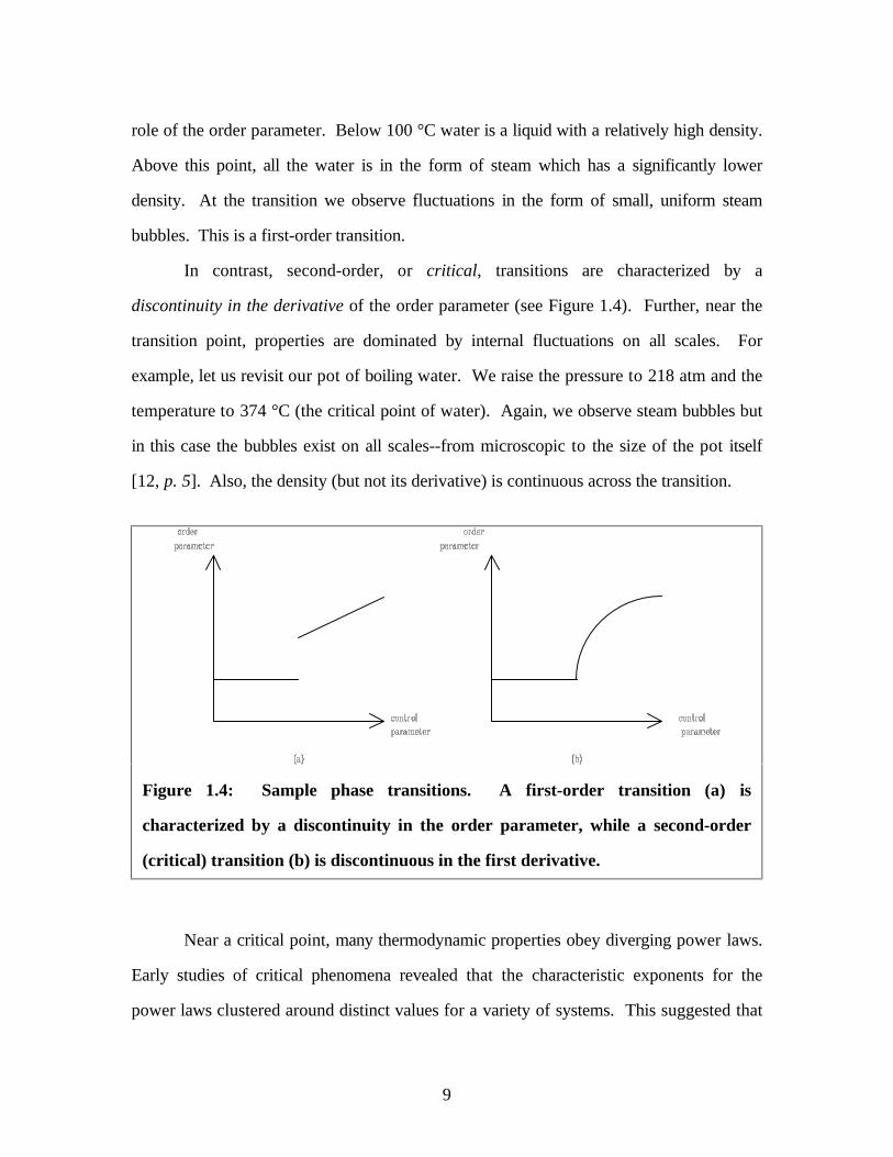
In contrast, second-order, or critical, transitions are characterized by a
discontinuity in the derivative of the order parameter (see Figure 1.4). Further, near the
transition point, properties are dominated by internal fluctuations on all scales. For
example, let us revisit our pot of boiling water. We raise the pressure to 218 atm and the
temperature to 374 °C (the critical point of water). Again, we observe steam bubbles but
in this case the bubbles exist on all scales--from microscopic to the size of the pot itself
[12, p. 5]. Also, the density (but not its derivative) is continuous across the transition.
Figure 1.4: Sample phase transitions. A first-order transition (a) is
characterized by a discontinuity in the order parameter, while a second-order
(critical) transition (b) is discontinuous in the first derivative.
Near a critical point, many thermodynamic properties obey diverging power laws.
Early studies of critical phenomena revealed that the characteristic exponents for the
power laws clustered around distinct values for a variety of systems. This suggested that
9

some of the features of separate systems were irrelevant --they belonged to the same
universality class. Some of the irrelevant variables in a universality class are usually the
type of local interactions, the number of nearest neighbors, et cetera. On the other hand,
dimensionality and symmetry, for example, appear to be relevant variables--that is, change
the number of dimensions or the symmetry laws and the system changes its class (or may
even cease being critical). Critical systems with the same relevant variables but different
irrelevant variables have the same critical exponents and are said to belong to the same
universality class. If GL can be determined to be critical it may be possible to determine
to which universality class it belongs, and hence, determine which variables are significant
and which are not.
1.3.2. Self-organization
Many natural systems exhibit self-organizing behavior: the formation of waterways, the
network of neurons in the human brain and the evolution of species are some examples.
All these spatially extended systems are governed by local interactions, yet they produce
interesting global structures. This is the essence of self-organization. Self-organizing
systems generate extreme anisotropy from initial randomness. In contrast, a gas also
interacts on a local level but in this case the interactions serve to disperse any
inconsistencies, bringing the system to equilibrium. Self-organized systems are sometimes
said to be far from equilibrium.
Often self-organization is called antichaos [13] because it appears to reduce
entropy, violating the second law of thermodynamics. In fact, this is not the case as all
systems exhibiting self-organization are driven by energy reserves. For example, the
process of evolution on earth is driven primarily by radiant energy from the sun.
However, it is possible to construct artificial models for which there exists no analogue for
energy. Such systems can exhibit self-organization without an obvious source. As we will
see, this is the case for GL.
10

1.3.3. Self-organized criticality
Self-organized criticality (SOC) is a merging of the two concepts above. Unlike the pot of
water in the example above, for which we had to deliberately adjust the temperature and
pressure to reach the critical state, SOC phenomena automatically approach the critical
state without any fine-tuning of external parameters. Although it may seem rare and
surprising, SOC actually appears to be fairly common in nature. It is seen in systems
having self-similar fractal structures [14] and in dynamics with 1 f (or flicker) noise.
Both these observed properties have been poorly understood in the past but now we
simply see them as manifestations of the power law behavior seen in critical phenomena.
In fact, spontaneously occurring flicker noise and fractal structures are the temporal and
spatial fingerprints of SOC seen in the light from quasars, the intensity of sunspots, the
current through resistors, the sand flow in an hourglass, the flow of rivers, stock market
fluctuations, cosmic structures and turbulence [15 and references therein].
Early studies explained SOC in terms of conserved quantities [1,2]. In particular,
exact results were achieved for a CA model of a sandpile in which the height of the pile
obeyed a local conservation law. It was assumed that conservation laws were integral to
SOC. Then Bak et al. [3] argued that GL also exhibited SOC. But, as we know, GL is
completely artificial, and obeys no known conservation laws--local or global. It was
argued that conservation was not a necessary property of SOC. But then doubt was cast
upon whether GL was SOC after all. Bennett and Bourzutschky [4] suggested that the
observed power law behavior was an artifact of the small system sizes explored in [3], and
on larger scales GL is actually subcritical. Alstrøm and Leão [5] countered, arguing that
the round-offs observed by [4] are boundary effects, and a finite-size scaling analysis
demonstrates GL is critical. The issue is still not resolved. Since then, Hemmingsson [6]
argued that the discrepancy in these results is a product of using different boundary
11

conditions and measuring different statistics. His results agree with those of Bennett and
Bourzutschky, that GL is not SOC.
In this paper we will explore whether GL is critical and if these conflicting analyses
can be reconciled. We will also explore how GL responds to some variations of control
parameters: whether it moves closer to--or further from--SOC.
12

2. Experimental Design
To study GL I needed a CA evolving program which was both fast and versatile. It must
be capable of handling a variety of boundary conditions; changing the dimensionality and
lattice size; recording either lattice configurations or just interesting statistics (to save disk
space); detecting and perturbing stable states; starting from either random or specific
initial lattice configurations; and perhaps most importantly, it must be adaptable to future
unforeseen uses. Unfortunately, I could not find any commercial or public domain
products that met all these requirements so I chose to design my own. The result is a
program I have unimaginatively dubbed CellBot, the source code of which is included in
Appendix A.
The source was coded on a personal computer running under MS-DOS. It was
compiled and debugged on the same computer with Borland Turbo C version 2.01 and
later with Borland C++ version 4.02. When sufficiently bug free the source was ported
over to a Sun SparcStation running under UNIX where it was recompiled and further
tested with Gnu C. Data acquisition runs were performed on four separate SparcStations.
Both compilers comply with the ANSI C standard and the resulting source code should be
very portable. CellBot should compile and run with any ANSI C compliant compiler in
virtually any operating environment.
Graphical interfaces which allow the user to visualize the CA as it evolves are
common among this type of program. However, I found it necessary to forgo this feature
for the sake of portability. Instead I chose to make the data for a visual display available
by recording all live cells in an ordinary text file accessible by a graphing program (I use
GnuPlot). One practical advantage this has is that it allows the user to back up. Many
CA (including GL) are time-irreversible: that is, multiple (degenerate) lattice
configurations can evolve to the same particular configuration in a single time step.
Unlike some other products, this set-up allows the user to travel back and forth through
the time line. Nevertheless, it would be gratifying to have a separate viewer program,
13

optimized for each operating environment, which directly read these data files and
graphically represented the system. It has been my personal experience that many subtle
bugs can be revealed by simply watching the system evolve. For example, the evolution
must obey the symmetries imposed by the transition rules (GL has a four-fold rotation and
reflection symmetry)--watching the lattice break symmetry constraints is the simplest way
of discovering bugs in the program. Perhaps the reader would be interested in developing
a viewer.
2.1. CA Subrules
CellBot can apply two separate subrules in each step of the CA's evolution. The first is
the standard local CA rule, mentioned above in the Introduction, applied synchronously.
The second, inspired by epidemic models [16], describing the motion of individual cells, is
applied sequentially.
2.1.1. Standard CA subrule
This subrule is described in the Introduction and Eq. (1.1). As it stands, CellBot only
accepts totalistic rules of the form given in Eq. (1.3). I have added one minor extension,
however. Each cell is selected for updating with some probability s, which is defined in
the rule file. If s=1 then the system is synchronous, but as s approaches zero fewer and
fewer cells are updated in each round. In the limit s→ 0, we effectively have a
completely asynchronous system.
We can call the evolution asynchronous if no neighboring cells are updated in the
same time step. The probability of a specific cell and any of its ℵ neighbors being
updated is given by the standard binomial expansion:
14

Pr( ( )cell & neighbors)=ℵF
HGIKJ
−
≅ ℵ
ℵ −
=
ℵ
∑s is s
s
i i
i
11
2
(2.1)
for small s. This is true for all of the N cells in the system. If, on average, less than one
synchronous update occurs per time step then the system is effectively asynchronous.
This suggests the system is effectively asynchronous if s sasync< where
sNasync = ℵ
. (2.2)
Let us consider as an example GL (ℵ = 8) on a 256×256 lattice. Then, the evolution
should be effectively the same as a completely asynchronous system if s s< =async 0 01105. .
However, it will be much more efficient than a truly asynchronous evolution because, on
average, 724 cells will be updated with each step. We must be careful with terminology
here: the rule itself is deterministic as discussed in Section 1.1, however, because it is not
applied uniformly, the global evolution may not be deterministic if s<1.
2.1.2. Mixing subrule
The second subrule allows the extension of CellBot to population models where the
motion of the individuals is an important factor in the global evolution such as epidemic
models [16] and population dynamics models [17]. After the standard CA subrule is
applied a fraction, m, of live sites are randomly moved to new (previously dead) positions.
Each cell can be moved only once.
The new position is randomly selected from all sites which lie within a distance Rm
for each degree of freedom. Note this restriction generates a cubic bounding box rather
than a spherical shell so that the number of available sites is
15
N Rm md= +( )2 1 (2.3)
where d is the dimensionality of the lattice (assuming there is no interference from the
boundaries). In this way, range of motion can be smoothly extended from short-range
(Rm = 1) to long-range (R Lm = , the length scale of the lattice).
CellBot allows for two methods of moving a cell. The first method simply uses a
uniform deviate to jump to a random new location within the above mentioned region. It
is computationally efficient but may not describe natural motion very well. Occupied or
out-of-bounds sites are not allowed, if an illegal site is chosen a new site is randomly
chosen. Note that the original site may be selected resulting in a null move. It is
important to consider under what circumstances this effect becomes relevant, or even
dominant. The probability of an illegal site being chosen in any single attempt is just the
average occupation density, c (neglecting boundary effects). The probability of a null
move on each attempt is 1Nm
and the probability of i failed moves followed by a null move
is 1 11N Ni i
m mc( )− . Hence, the effective mixing fraction is scaled down by the fraction of
null moves:
m m c
mN c c
effjump
N Ni i
i
m
m m= − −
L
NM
O
QP
= −− +
L
NM
O
QP
=
∞
∑1 1
11
1
1 1
0
( )
( )
(2.4)
by the geometric series. As an example, let us consider GL (c = 0 03. ) with short-range
mixing (Nm = 9). In this case, m meffjump ≅ 0 885. .
The other method of mixing uses a random walk of Rm steps. In each step a new
site in the current site's neighborhood, ℵ, is chosen. Note that CellBot allows the user to
configure the neighborhood in any way, the sites need not even be contiguous or
symmetric. This fact, and the fact that the probabilities for motion in orthogonal
directions are not independent, make this random walk problem difficult to analyze.
Hence, we make the leap of faith that the results for the paradigmatic one-dimensional
16

random walk problem [18, pp. 7-24] apply here as well. This tells us the root-mean-
square distance traveled in a random walk is proportional to the root of the number of
steps so we can determine the average distance a cell will be moved:
d r c Rmwalk
step m= ( ) (2.5)
where we define the average distance moved in a single step as
r cc
step( )( )
= −ℵ + ∈ℵ
∑11
xx 0
. (2.6)
The 1− c factor arises because a cell will not move into an already occupied site, and the
denominator is incremented by one because the null move is allowed. For GL this
definition gives rstep( . ) .0 03 1 0408= .
The classical random walk also predicts that the probability distribution will have a
Gaussian form with a ( )2πσ −d prefactor where the standard deviation, σ, is equal to the
root-mean-square distance travelled. The probability of no net movement is just this
prefactor so we can estimate the effective mixing fraction by scaling it down by the
probability that no net movement occurs:
m mR
effwalk
m
d≈ −L
NMM
O
QPP
11
2 2πb g. (2.7)
Of course, this estimate needs to be taken with a grain of salt, and has no numerical worth
in itself. A better result would be obtained by determining the probability distribution
explicitly for the particular geometry one wishes to study. However, this information
would be of minimal use in this paper so it is left as an exercise for the reader. (I've
always wanted to say that!)
The random walk method may seem preferable because it seems more natural, but
there are instances when the jump method is preferred. For example, the average distance
moved via the jump method for long-range mixing on a square lattice of side L is
d Lmjump = 2
3 . To achieve this range with the walk method would require
17
RL
r cmstep
= 2
9
2
( )(2.8)
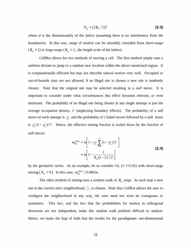
or, on a 256×256 lattice, 14,564 steps. Obviously, this would greatly reduce program
performance. The random walk method is best suited to shorter-range motion.
In both cases above, the results are slightly complicated by the fact that the
dynamics, and hence the average occupation density, depend on the mixing fraction, m, so
that c c m= ( ), as we will see in the next section. Hence, the numerical values of meff
given may be inaccurate. However, this is not a serious problem as c can be determined
experimentally and the resulting values used in the above formulas. Also, in the
derivations we assumed uniform probability densities when we know GL exhibits extreme
spatial inhomogeneity. As we will see, though, mixing has the effect of randomizing the
distribution and inducing uniform probabilities, so this should be valid for m ≠ 0.
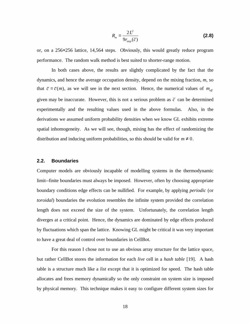
2.2. Boundaries
Computer models are obviously incapable of modelling systems in the thermodynamic
limit--finite boundaries must always be imposed. However, often by choosing appropriate
boundary conditions edge effects can be nullified. For example, by applying periodic (or
toroidal) boundaries the evolution resembles the infinite system provided the correlation
length does not exceed the size of the system. Unfortunately, the correlation length
diverges at a critical point. Hence, the dynamics are dominated by edge effects produced
by fluctuations which span the lattice. Knowing GL might be critical it was very important
to have a great deal of control over boundaries in CellBot.
For this reason I chose not to use an obvious array structure for the lattice space,
but rather CellBot stores the information for each live cell in a hash table [19]. A hash
table is a structure much like a list except that it is optimized for speed. The hash table
allocates and frees memory dynamically so the only constraint on system size is imposed
by physical memory. This technique makes it easy to configure different system sizes for
18

each run, and in fact, even the dimensionality can be configured. For sparse lattices (as in
GL), this design also offers a performance advantage because fewer cells need to be
updated in each step of a run. Note that the choice of rules in CellBot is constrained by
this design. Since CellBot ignores dead sites with all dead neighbors it is imperative that
the transition rule maps these configurations to dead.
Boundaries are imposed artificially by inserting the appropriate cells beyond the
bounds of the system before each update. In the current version of CellBot, boundaries
are simply defined by minimum and maximum coordinates (inclusive). A variety of
boundary types can be chosen and even intermixed. For example, periodic boundaries in
one dimension can be mixed with reflective boundaries in another (see Figure 2.1).
Corner disputes are managed by assigning priorities to the various boundaries; the side
with the highest priority imposes its boundary type on the corner. Currently, CellBot
supports cold (all cells beyond border are dead), hot (a fraction, h, of cell's beyond the
border are alive), periodic, reflective, and even no boundaries.
19
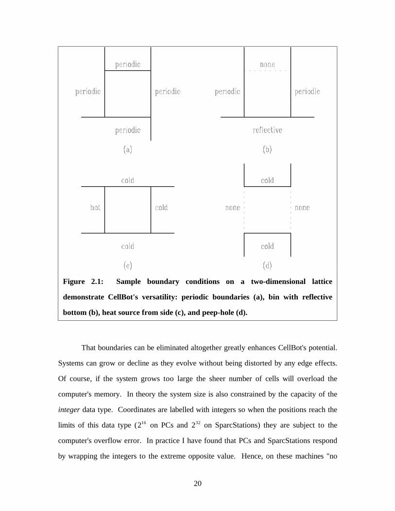
Figure 2.1: Sample boundary conditions on a two-dimensional lattice
demonstrate CellBot's versatility: periodic boundaries (a), bin with reflective
bottom (b), heat source from side (c), and peep-hole (d).
That boundaries can be eliminated altogether greatly enhances CellBot's potential.
Systems can grow or decline as they evolve without being distorted by any edge effects.
Of course, if the system grows too large the sheer number of cells will overload the
computer's memory. In theory the system size is also constrained by the capacity of the
integer data type. Coordinates are labelled with integers so when the positions reach the
limits of this data type (216 on PCs and 232 on SparcStations) they are subject to the
computer's overflow error. In practice I have found that PCs and SparcStations respond
by wrapping the integers to the extreme opposite value. Hence, on these machines "no
20

boundaries" effectively means periodic boundaries with a length scale of L=65536 and
L=4294967296, respectively. My data-gathering runs were all performed on
SparcStations at a rate on the order of ten time steps per second. At this rate, the effect of
the boundaries would not be felt for some ten years, well beyond the period of this project,
making this system effectively infinite.
When implementing different boundary combinations it is best if unbounded edges
receive the lowest priority (as in Figure 2.1(b)). A bug in the program may prevent
submissive hot, periodic, and reflective boundary types from behaving in the expected
manner along these edges. One could not, for example, impose boundaries simulating two
large reserves separated by a small peep-hole, like that in Figure 2.1(d), unless it was with
cold boundaries.
CellBot is biased towards rectangular lattices by the boundary conditions. When
studying other geometries, like triangular neighborhoods, it is best not to impose
boundaries for fear of introducing some artifact of this bias (see Figure 2.2). In particular,
periodic boundaries will behave very poorly, associating cells on opposite edges with sites
the user may not expect. This defect is not a problem here, because GL lies on a
rectangular lattice, but it should be remedied for future research.
21
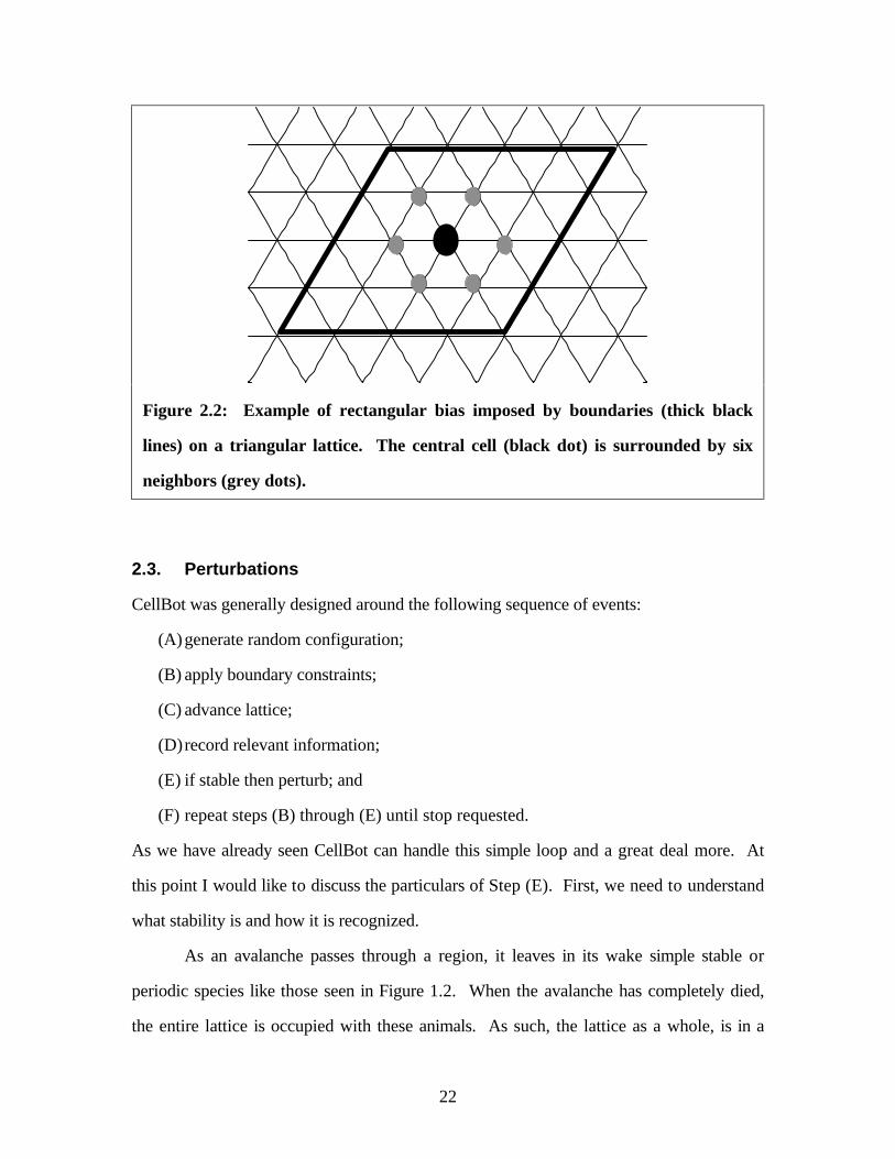
Figure 2.2: Example of rectangular bias imposed by boundaries (thick black
lines) on a triangular lattice. The central cell (black dot) is surrounded by six
neighbors (grey dots).
2.3. Perturbations
CellBot was generally designed around the following sequence of events:
(A)generate random configuration;
(B) apply boundary constraints;
(C) advance lattice;
(D)record relevant information;
(E) if stable then perturb; and
(F) repeat steps (B) through (E) until stop requested.
As we have already seen CellBot can handle this simple loop and a great deal more. At
this point I would like to discuss the particulars of Step (E). First, we need to understand
what stability is and how it is recognized.
As an avalanche passes through a region, it leaves in its wake simple stable or
periodic species like those seen in Figure 1.2. When the avalanche has completely died,
the entire lattice is occupied with these animals. As such, the lattice as a whole, is in a
22
periodic pattern. We call such a configuration stable. In practice, naturally occurring
configurations tend to have very short periods, typically from two to six time steps.
To detect stable states one usually uses a moving window to compare the current
lattice with those for the last pmax time steps. This allows for the detection of periodic
configurations with periods up to pmax. This method suffers from two drawbacks: firstly,
the memory consumed by the storage of the lattice history may be enormous. Secondly,
comparing two lattices for a match site-by-site would significantly reduce system
performance. I chose to implement a slightly different method. Instead of a moving
window of lattice configurations, I merely store, in a moving window, a particular statistic
which is very sensitive to the lattice state. It is important that the statistic of choice is not
easily reproducible by different configurations in order to minimize the chance of the
program erroneously declaring the lattice stable. Further, the history contains the last
2pmax values of the statistic and requires the entire sequence to match before admitting the
lattice is stable. The chance of a false positive is negligible (I have never encountered one
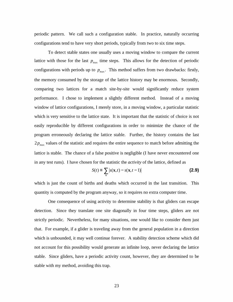
in any test runs). I have chosen for the statistic the activity of the lattice, defined as
S t s t s t( ) ( , ) ( , )≡ − −∑ x xx
1 (2.9)
which is just the count of births and deaths which occurred in the last transition. This
quantity is computed by the program anyway, so it requires no extra computer time.
One consequence of using activity to determine stability is that gliders can escape
detection. Since they translate one site diagonally in four time steps, gliders are not
strictly periodic. Nevertheless, for many situations, one would like to consider them just
that. For example, if a glider is traveling away from the general population in a direction
which is unbounded, it may well continue forever. A stability detection scheme which did
not account for this possibility would generate an infinite loop, never declaring the lattice
stable. Since gliders, have a periodic activity count, however, they are determined to be
stable with my method, avoiding this trap.
23

Once CellBot determines a configuration is stable, it tries to incite activity by
perturbing a single site. The site can be either dead or alive, the perturbations flips it to
the contrary state. The result is an avalanche as the lattice tries to recover from the
disturbance. The perturbation site is recorded in the data file. Actually, perturbations can
be applied at regular intervals, not just after the system has stabilized. The latter choice is
equivalent to setting the perturbation rate to zero.
As mentioned above, the perturbations implemented are of the form of a reversal
of a single site. Other kinds of perturbations may be useful, as well. For example,
constructing gliders and sending them into the system provides a method of perturbation
which has the advantage of conforming to GL's rules. A single site perturbation violates
these rules by spontaneously creating or destroying a cell. A glider, however, could be
interpreted as coming from a source at a very large distance, hence, it is consistent with
GL's rules. It is not clear whether this or other types of perturbations would modify the
dynamics, but they are not implemented in this version of CellBot.
Perturbations will be discussed in more detail in Section 3.2.1.
24
3. Finite-size scaling
3.1. Introduction
Science in general, is divided into a number of subjects. At first look these subjects may
seem unrelated: physics is distinct from biology which is distinct from chemistry, et cetera.
A better interpretation, however, perhaps may view the separate fields as layers
surrounding a central core--like the layers of an onion. These layers are separated by
complexity barriers, At the core lie the "theories of everything" which attempt to describe
all the fundamental interactions in physics. Perhaps the next shell contains the Standard
Model of sub-atomic particles. Beyond this we find chemistry, dealing with atoms and
molecules. Jumping to the next layer we might find biochemistry, the study of complex
molecules like proteins and how they interact. Continuing on our biological bent, we
expect to find cellular biology and the study of unicellular organisms. This layering
interpretation can be extended indefinitely to include (almost) all science. But what
separates these layers? The answer is complexity. While in principle it may be possible to
describe biomolecular processes in terms of quarks and gluons, in practice it is impossible
because of the sheer volume of interacting particles which make up each protein. Having
a "theory of complexity" which allows one to reliably extend the basic principles of a
fundamental theory to a higher level, at least in isolated cases, could be very
advantageous. Any such theory would serve as a link between theories on two successive
levels, and by verifying a known phenomenon, would strengthen both theories.
One may wonder why we are interested in GL at all. It has no basis in reality.
While it is true GL generates interesting dynamical patterns it doesn't tell us anything
about ourselves or the world around us. Or does it? GL is an example of a complex
system arising from simple local interactions. There are many natural phenomena with the
same criteria. Perhaps, if we can make some headway in exploring GL then the techniques
we discover can be adapted to more complex natural systems. GL can serve as a litmus
25

test for theories of complexity--both analytic theories and computer simulations. Until we
have made some headway in the investigation of the Game of Life we can not expect to
understand the complexities of life.
In essence, GL is simply a many-body system with local interactions. There are
many exact and approximate methods of solving many-body problems so one may suspect
that analysis would be a fairly simple procedure. However, on closer inspection we see
that many of the tools at hand are inapplicable for one insurmountable reason or another.
One of the main problems for analysis is the lack of a local conservation law. The sandpile
model was solved exactly via renormalization-group calculations precisely because of the
local conservation law [2]. Further, with a conserved quantity it would be possible to
construct a free energy and a Hamiltonian. This would greatly enhance the range of tools
at our disposal. Other peculiarities of GL (like the fact that it is deterministic, not
stochastic) invalidate other potential tools. The most successful method for studying GL
has been to search for the characteristic power law behavior of thermodynamic quantities
near a critical point.
Just like the pot of boiling water at the critical point had bubbled of all sizes,
critical system are characterized by events of all sizes. The frequency distribution of these
events scales as a power law of the size. One fairly simple way to determine if a system is
critical is by directly searching for the characteristic power law behavior in some global
quantity of the system. We will apply this as our first angle of attack. A simple and
effective quantity to explore in GL is the size of an avalanche (or time required to re-
stabilize) arising from a perturbation. The basic algorithm runs as follows:
(A) randomly seed lattice, wait for stabilization;
(B) perturb lattice and wait for re-stabilization;
(C) record stabilization time;
(D)repeat (B) and (C) until sufficient statistical population acquired.
26

When a good statistical data set has been collected the points are grouped by size and the
resulting distribution is compared to the suspected power law.
3.2. Considerations
At this point it may seem a simple procedure to make a few thousand runs, get a nice
statistical distribution, and test the power law distribution, but in fact, there are a few
details which first require our attention.
3.2.1. Perturbations
We must be careful the nature of the dynamics does not arise from the particulars of the
perturbation algorithm, but from some intrinsic property of the system itself. Following
example [3,20,4,5,6], we implement perturbations by choosing a random site and flipping
its state from dead to alive or vice versa.
There are two points of consideration here. Firstly, notice that GL has a lattice
occupancy of about 3%. If we chose our perturbation site completely randomly then the
chance of choosing a dead zone (a dead site surrounded by all dead neighbors) is roughly
0 97 0 769. .≅ . But GL's rules tell us such a perturbation will result in a flip-fail (the lattice
immediately reverts back to its original configuration) and the avalanche will be recorded
as having lifetime one time step. This will not adversely affect the shape of the frequency
distribution, but it will produce a large spike at the low end, completely obscuring any true
data for avalanches of size one. Hence, it would be necessary to ignore the low end when
analyzing the distribution. The only real problem here is that this leaves us with only 24%
of our original data for analysis. It would be more efficient if we could choose our
perturbation sites more effectively in order to minimize flip-fails. This is what I have
done. I choose a perturbation site from a list of all live cells and those sites in their
collective neighborhood. This guaranties the perturbation site will always have at least
27

one live cell in its neighborhood--generating roughly a four-fold increase in productive
data.
The second issue of concern also relates to the location of the perturbations.
There is a possibility that the evolution of an avalanche depends on the depth of the locus
within a cluster. That is, perturbations on the surface of a cluster may evolve differently
than perturbations within the body. To test this I compared the lifetimes of avalanches to
their locus, the perturbation site. To avoid boundary effects I analyzed data from a GL
run that lacked boundaries (see Section 3.12 for more details on this run). Plotting the
lifetimes of perturbations against the radial distance of the perturbation sites from the
center of mass, a flat line would indicate that the avalanche dynamics were independent of
the depth of the perturbation site. Of course, suspecting that GL may be critical we know
that there may be a large deviation in avalanche sizes, even for very similar perturbations.
Indeed this is what the plot revealed so I needed a smoothing technique which would
reveal the underlying average behavior. I chose to use a numerical integration which
smoothes nicely, but has the effect of converting flat lines into straight lines with non-zero
slopes. The results are shown in Figure 3.1. The x-axis represents the radial distance of
the perturbation site from the center of mass scaled by the characteristic length of the
system, L (defined in Section 3.12.1), and the y-axis represents the integral of the
perturbation lifetimes. Notice that, for perturbations within about 10L of the center the
plot fits a straight line fairly well suggesting that, in this region, avalanche dynamics are
independent of the perturbation site--there do not appear to be any surface effects
complicating the picture. (It appears that for avalanches very near the center, within 0.3L,
there is a slight decrease in avalanche activity. It is unclear whether this is a significant
effect or simply a statistical fluctuation. In any case, the deviation is slight, so I will call
no further notice to it.)
28

0
20
40
60
80
100
120
140
0 0.2 0.4 0.6 0.8 1
cum
ulat
ive
lifet
ime
distance from center
0
500
1000
1500
2000
2500
0 5 10 15 20 25
cum
ulat
ive
lifet
ime
distance from center
(a) (b)
Figure 3.1: Numerical integral of avalanche lifetimes plotted against radial
distance of locus from center of mass. Distances are scaled to the characteristic
size of the system. The relatively straight line in (a) indicates avalanche lifetimes
do not depend on the perturbation site, at least up to the size of the system. On
scales much larger than the system (b) avalanches do appear to be affected by the
perturbation site, but the results are not statistically reliable.
Beyond this length scale, however, the figure implies there are some surface
effects. This is not necessarily the case as the results in this region are statistically
unreliable. Most live cells reside in clusters near (within radius L) of the center. Hence,
perturbations using the method described above will occur with dropping frequency
beyond the system size. For very large radii the perturbations are few and far between.
More data points may smooth out the plot shown in Figure 3.1(b) or, on the other hand,
they may reveal more interesting dynamics. Perhaps this area is worth further study but
most of the systems studied in this paper will be bounded so I will leave it be.
3.2.2. Transient length
When starting a run the lattice is initially seeded with a random population (usually with
density 0.5). The system evolves to a stable state and is perturbed at a single site. As the
29
process is repeated, the system evolves into a statistically stationary state, which does not
depend on the initial configuration. The properties of this state are the object of our
investigations. As such we must consider the possibility of a transient–an intermediate
behavior as the system slowly obscures information regarding the initial configuration
(remember, GL is irreversible). Some artifact of the seed may remain for many
perturbations after. For example, the spatial distribution of species may be more uniform
initially, but become more clustered in the statistically stationary limit. When analyzing
GL we would like to skip the polluted data from this transient period.
If there is a transient period it should be observable by looking at the evolution of
some statistical property (order parameter) of the run. Figure 3.2 shows the temporal
(measured by the number of perturbations) evolution of the number of live sites. The raw
data is smoothed via a "moving window average" in which each point is average with the
first 128 points on either side. The figure suggests that there is no transient period,
whatsoever. That is, the system reaches its limiting behavior immediately upon settling
down from the initial seed. This is good news because it means all of our acquired data is
available for analysis.
30

200
250
300
350
400
450
500
550
600
650
0 2000 4000 6000 8000 10000
live
cells
perturbations
Figure 3.2: Demonstration that GL exhibits no transient behavior. The points
show the evolution of the number of live cells over time (perturbations). The line
represents a moving window average of width 257 points. Results are for a
128 128× periodic lattice.
3.3. Critical exponents: variable-width bins
We are now in a position to test GL for critical behavior. As mentioned above, we are
interested in the frequency distribution of avalanche lifetimes, t. If GL is SOC the
frequencies of lifetimes should decay via a power law with the lifetimes
D t tb( ) ∝ (3.1)
where b is called a critical exponent. (We expect b<0.) The power law behavior can be
seen by plotting the distribution on a log-log graph, so that the power law is mapped to a
straight line with a slope b. For statistically stable results a great deal of data points is
31
required. I found a typical run containing ten thousand avalanches produces a sufficiently
smooth distribution. In the following runs I employed periodic boundary conditions.
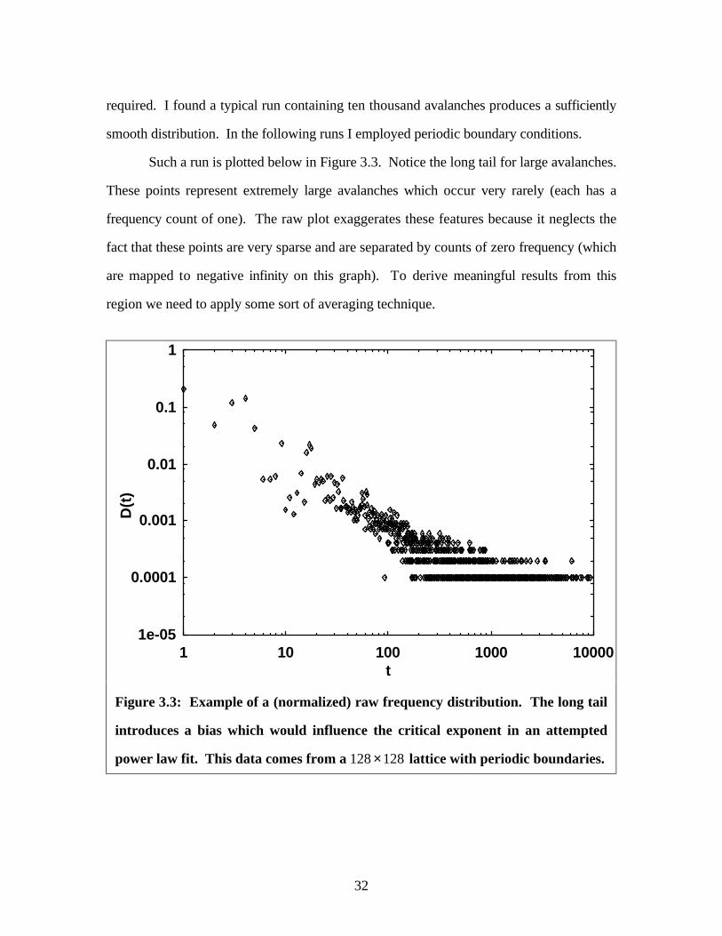
Such a run is plotted below in Figure 3.3. Notice the long tail for large avalanches.
These points represent extremely large avalanches which occur very rarely (each has a
frequency count of one). The raw plot exaggerates these features because it neglects the
fact that these points are very sparse and are separated by counts of zero frequency (which
are mapped to negative infinity on this graph). To derive meaningful results from this
region we need to apply some sort of averaging technique.
1e-05
0.0001
0.001
0.01
0.1
1
1 10 100 1000 10000
D(t
)
t
Figure 3.3: Example of a (normalized) raw frequency distribution. The long tail
introduces a bias which would influence the critical exponent in an attempted
power law fit. This data comes from a 128 128× lattice with periodic boundaries.
32
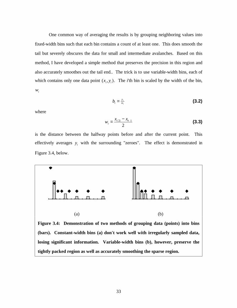
One common way of averaging the results is by grouping neighboring values into
fixed-width bins such that each bin contains a count of at least one. This does smooth the
tail but severely obscures the data for small and intermediate avalanches. Based on this
method, I have developed a simple method that preserves the precision in this region and
also accurately smoothes out the tail end.. The trick is to use variable-width bins, each of
which contains only one data point ( , )x yi i . The i 'th bin is scaled by the width of the bin,
wi
biyw
i
i= (3.2)
where
wx x
ii i= −+ −1 1
2(3.3)
is the distance between the halfway points before and after the current point. This
effectively averages yi with the surrounding "zeroes". The effect is demonstrated in
Figure 3.4, below.
(a) (b)
Figure 3.4: Demonstration of two methods of grouping data (points) into bins
(bars). Constant-width bins (a) don't work well with irregularly sampled data,
losing significant information. Variable-width bins (b), however, preserve the
tightly packed region as well as accurately smoothing the sparse region.
33

Using this grouping method on the data in Figure 3.3 reveals the distribution's
underlying power law behavior (dots in Figure 3.5). The graph also shows a line which
represents the data smoothed with a low-pass Savitsky-Golay smoothing filter [7]. This
filter fits each data point and the nearest 32 points on either side to a polynomial of degree
one (a straight line) via a linear least-squares fit on the log-log graph . Fitting this curve to
a straight line on the log-log scale may impose an artificial bias towards a power law so
the resulting smoothed data is used subsequently only for graphing purposes. For
calculations the binned (but not smoothed) data is used.
1e-07
1e-06
1e-05
0.0001
0.001
0.01
0.1
1
1 10 100 1000 10000
dist
ribut
ion,
D(t)
lifetime, t
Figure 3.5: Binned lifetime distribution for 128 128× periodic system (see Figure
3.3). The line represents the smoothed data using a Savitsky-Golay (32,32,1)
filter. Notice the drop-off for large avalanches.
Notice, contrary to the raw plot (Figure 3.3), there appears to be a decay from the
power law behavior at large time scales. This deviation has been observed by others [5,6]
and is central to the problem of whether GL is critical. As such I am confident it is not an
artifact of my averaging method. At this point we assume the deviation is due to the
34

relatively small lattices explored. To estimate the best power law fit, then we must ignore
the tail, discarding t>1000.
We also expect the extremely small time scales to cause problems. At this scale
the discreteness of the time steps may interfere with the natural distributions of lifetimes.
Hence, as a precaution, we also discard data for t<20. As it stands, this should make little
difference in the calculations, as these are only 20 points out of some thousands.
Barring these constraints, the plot does indeed seem to fit a power law distribution.
The only other point to consider is that the results shown are for a single run on a lattice
with a particular length. If GL is critical the above results should hold true for any
reasonably sized lattice, and further, the power law parameters should be independent of
the lattice size. To test this, a series of runs with differing lengths were analyzed and the
results are shown in the figure below. Indeed, the data does appear to conform with a
power law distribution, at least within the range mentioned above. In this region the
average critical exponent (see Eq. (3.1)) is estimated to be b = − ±1 175 0 012. . .
35

1e-07
1e-06
1e-05
0.0001
0.001
0.01
0.1
1
1 10 100 1000 10000
dist
ribut
ion,
D(t)
lifetime, t
power-law fitL=64L=91
L=128L=181L=256
Figure 3.6: Overlapping plot of lifetime distributions for L L× periodic lattices.
The data has been smoothed with a Savitsky-Golay smoothing filter (32,32,1).
The average power law fit critical exponent (computed between t=20 and t=1000)
is b=-1.175+0.012.
Two previous measures of this quantity gave b ≈ −1 6. [3] and b = −1 41. [5]. It is
odd that none of these values agree very closely. It appears Bak et al. [3] did not exclude
either the low end of the distribution, which is polluted by discreteness, or the high end of
the distribution, which is polluted by finite-size effects, when estimating their critical
exponent. Further, they only explored lattices with cold boundaries up to 150 150× ,
which may suffer from extreme corrections to scaling. This may account for the
discrepancy seen with their result. Alstrøm and Leão [5], however, corrected for both
aberrations and they tested lattices up to 1024 1024× . The only difference is that they,
too, applied cold boundaries, but I am hesitant to attribute the difference in our critical
exponents to this fact. This discrepancy hinted that something deeper may be occurring,
and it led me to apply another method for determining the critical exponents.
36
3.4. Critical exponents: cumulative distribution
The disagreement noted above suggested that there may be a flaw in my technique. It was
first suspected that the problems arised from a nuisance parameter in the fit. When fitting
the binned data to a power-law there are three variables which must be adjusted to get a
good fit: the critical exponent (slope, b), the normalization factor (y-intercept), and the
high-end cutoff (which we set to 1000). Of these we are only interested in the exponent,
b. The other variables are termed nuisance parameters because they must be properly
adjusted when fitting, but are discarded afterwards. Because a model involving fewer
adjustable parameters is considered to have more validity, nuisance parameters impair the
confidence one has in a model.
It was proposed that the normalization factor, a nuisance parameter, may be
unduly influencing the parameter of interest, the critical exponent. For example, the
normalization factor may be estimated too small, decreasing the estimated slope. (In fact
we will discover the problem lies elsewhere, I only want to relay the historical
development of the new method here.) It is possible to discard the normalization factor
with a simple adjustment: instead of analyzing the lifetime distribution, we analyze the
cumulative distribution of lifetimes, C t( ) . The cumulative distribution is defined as the
fraction of avalanches larger than (or equal to) some lifetime, t:
C t D tt t
( ) ( )= ′′≥∑ . (3.4)
By this definition, C( )1 1= because D t( ) is normalized. Hence, we have eliminated one
of the nuisance parameters by setting it to one. Another advantage of working with the
cumulative distribution is that it acts as a smoothing function, reducing the noise seen in
the original distribution. Further, the cumulative distribution is compiled from the original
data (see Figure 3.3), not the binned data which has come under suspicion. These
attributes make the cumulative distribution an ideal candidate for analysis.
37
3.4.1. Finite-scaling preview
In the following analysis the determination of the critical exponent is integrated with
estimation of finite-size effects. It is necessary to introduce the reader to the concept of
finite-size scaling. We assume the distribution of lifetimes in the finite system (Eq. (3.1)
represents the infinite system) can be written as
D t t f tt LL
b
c( ) ( )∝
(3.5)
where f, the scaling function, obeys f x( ) → 1 for x<<1 and f x( ) → 0 for x>>1. This
form was originally hypothesized in 1969 and has been used successfully in many cases to
extrapolate systems near a critical point [12 and references therein]. The critical lifetime,
tc, which depends on the system length, L, represents the avalanche size above which
dynamics are dominated by finite-size effects (boundaries). (The assumption is that
longer-lasting avalanches are more likely to interact with the boundaries.)
The cumulative distribution, then, also obeys a finite-scaling law of the form
C t t g tt
b
c( ) =
+1 (3.6)
where the scaling functions f and g obey the relation
f x b g x xg x( ) ( ) ( ) ( )∝ + + ′1 . (3.7)
Notice the equality symbol in Eq. (3.6), indicating we have eliminated the nuisance
parameter. Without loss of generality (because the scaling function is strictly positive) we
can write g as an exponential:
g x eh x( ) ( )= . (3.8)
The goal is to fit the data to the simplest possible form of h. To determine the form of h
we expand it in a Taylor polynomial:
h x h h x( ) = + +0 1 K. (3.9)
But we know, from the restriction C( )1 1= , that h0 0= .
38
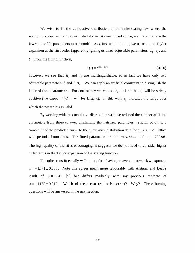
We wish to fit the cumulative distribution to the finite-scaling law where the
scaling function has the form indicated above. As mentioned above, we prefer to have the
fewest possible parameters in our model. As a first attempt, then, we truncate the Taylor
expansion at the first order (apparently) giving us three adjustable parameters: h1 , tc , and
b. From the fitting function,
C t t eb h t tc( ) = +1 1 (3.10)
however, we see that h1 and tc are indistinguishable, so in fact we have only two
adjustable parameters: b and h tc1 . We can apply an artificial constraint to distinguish the
latter of these parameters. For consistency we choose h1 1= − so that tc will be strictly
positive (we expect h x( ) → −∞ for large x). In this way, tc indicates the range over
which the power law is valid.
By working with the cumulative distribution we have reduced the number of fitting
parameters from three to two, eliminating the nuisance parameter. Shown below is a
sample fit of the predicted curve to the cumulative distribution data for a 128 128× lattice
with periodic boundaries. The fitted parameters are b = −1378544. and tc = 1792 96. .
The high quality of the fit is encouraging, it suggests we do not need to consider higher
order terms in the Taylor expansion of the scaling function.
The other runs fit equally well to this form having an average power law exponent
b = − ±1371 0 008. . . Note this agrees much more favourably with Alstrøm and Leão's
result of b = −1 41. [5] but differs markedly with my previous estimate of
b = − ±1175 0 012. . . Which of these two results is correct? Why? These burning
questions will be answered in the next section.
39
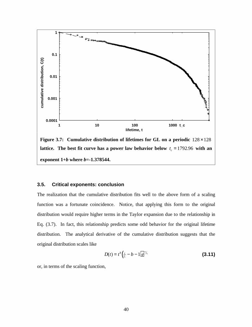
0.0001
0.001
0.01
0.1
1
1 10 100 1000 t_c
cum
ulat
ive
dist
ribut
ion,
C(t
)
lifetime, t
Figure 3.7: Cumulative distribution of lifetimes for GL on a periodic 128 128×
lattice. The best fit curve has a power law behavior below tc = 1792 96. with an
exponent 1+b where b=-1.378544.
3.5. Critical exponents: conclusion
The realization that the cumulative distribution fits well to the above form of a scaling
function was a fortunate coincidence. Notice, that applying this form to the original
distribution would require higher terms in the Taylor expansion due to the relationship in
Eq. (3.7). In fact, this relationship predicts some odd behavior for the original lifetime
distribution. The analytical derivative of the cumulative distribution suggests that the
original distribution scales like
( )D t t b eb ttc
ttc( ) = − −
−
1 (3.11)
or, in terms of the scaling function,
40

f tt
t
t be
cc
ttc
= −
+
−
11( )
. (3.12)
The linear factor in the scaling function counters the drop-off produced by the decaying
exponential, generating a hump near tc (see the figure below). This is very unusual
behavior for a scaling function. Traditionally, we expect the function to be monotonically
decreasing from one to zero. Nevertheless, it still satisfies the scaling function
requirement that as tc → ∞ , f converges to one for all t.
0.01
0.1
1
10
1 10 100 1000 10000
scal
ing
func
tion,
f(t)
lifetime, t
Figure 3.8: Weight of finite-scaling function of original lifetime distribution, f,
with model parameters b = −1378544. and tc = 1792 96. (corresponding to
periodic 128 128× run). Note the hump near tc .
The effect of the rise in the scaling function is to artificially inflate the lifetime
distribution, near tc , above the true power law. Hence, fitting the raw data to a power
law while not taking this factor into account will result in an erroneous critical exponent.
Now we understand this as the source of the discrepancy in the two measures of the
41

critical exponent. When we originally fit the binned distribution to a power law with a
cut-off we did not expect this unusual behavior from the scaling function and, as a result,
estimated too small an exponent. We conclude that the correct power law exponent is the
latter estimate of b = − ±1371 0 008. . , in agreement with Alstrøm and Leão's result.
Having established the proper form of the scaling function we can compare the
binned data (which generated our first, inaccurate measure of b) to the predicted curve in
Eq. (3.11). The use of variable-width bins came under suspicion when we observed the
disparity in our results. The figure below redeems the method, showing a very good fit.
This confirms that the source of error lies only with the unusual form of the scaling
function observed above. Note that, given the variance of the distribution, it is very
difficult to be sure of one's model and fitted parameters. The cumulative distribution, on
the other hand, smoothes the data and reduces the noise level, giving a much stricter data
set and making it easier to test the validity of potential models. We will discuss the
variance (noise) of the distribution further in Section 3.8.
42
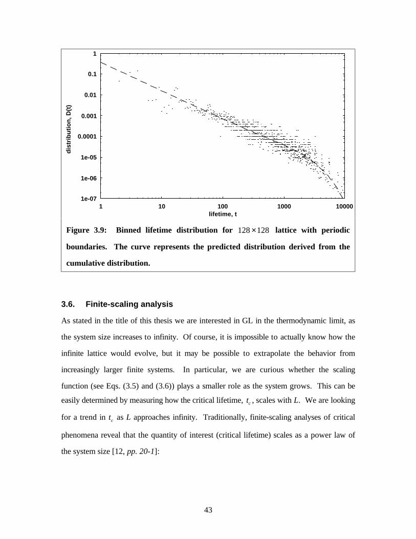
1e-07
1e-06
1e-05
0.0001
0.001
0.01
0.1
1
1 10 100 1000 10000
dist
ribut
ion,
D(t
)
lifetime, t
Figure 3.9: Binned lifetime distribution for 128 128× lattice with periodic
boundaries. The curve represents the predicted distribution derived from the
cumulative distribution.
3.6. Finite-scaling analysis
As stated in the title of this thesis we are interested in GL in the thermodynamic limit, as
the system size increases to infinity. Of course, it is impossible to actually know how the
infinite lattice would evolve, but it may be possible to extrapolate the behavior from
increasingly larger finite systems. In particular, we are curious whether the scaling
function (see Eqs. (3.5) and (3.6)) plays a smaller role as the system grows. This can be
easily determined by measuring how the critical lifetime, tc , scales with L. We are looking
for a trend in tc as L approaches infinity. Traditionally, finite-scaling analyses of critical
phenomena reveal that the quantity of interest (critical lifetime) scales as a power law of
the system size [12, pp. 20-1]:
43
t Lcz∝ (3.13)
where z is called the finite-scaling exponent. Hence, the scaling function, f, approaches
one for all t as L increases.
The results for square, periodic lattices of various lengths is plotted below. It
appears that GL scales for small L (with scaling exponent z = ±0 355 0 015. . ) but stabilizes
at tc = ±1981 17 as L increases past 181. This suggests that this configuration probably
has a correlation length ξ ≈ 181 below which the dynamics are dominated by edge effects,
but above which boundaries play a minimal role. Having only one data point above the
transition makes impossible to extrapolate the behavior with any degree of reliability. It is
possible that above the transition, the critical lifetime again scales with L but has a much
smaller scaling exponent. More data is required to positively identify the large-scale
behavior. I am currently collecting further data on larger lattices, but the results were not
available in time for this paper.
44

1000
2000
3000
32 64 128 256 512
criti
cal l
ifetim
e, t_
c
system size, L
Figure 3.10: Finite-size scaling plot for GL on a square lattice with periodic
boundaries. The finite-scaling exponent for small L is z = ±0 355 0 015. . but GL
does not appear to scale for L ≥ 181.
Although our previous calculation of the critical exponent agreed closely with
Alstrøm and Leão's [5], their finite scaling analysis contrasts sharply with the above graph.
They conclude that GL does indeed scale with L, with a scaling exponent z ≅ 0 52. . There
are three possible explanations for this: firstly, they studied GL on square lattices with
open (or cold) boundaries. We expect edge effects to be more severe for these systems so
it may be that GL scales as a power law beyond the maximum lattice size they studied
(1024 1024× ). The transition to a constant critical lifetime may occur above L=1024.
The second possible explanation is that the level of noise in the distributions
reduced the accuracy of their results. It is not an attractive alternative, but I see no
account made of the variance in the data so I can not exclude it as a possibility. Their runs
consisted of a quantity of data points on the same order as mine, so the variance in their
data should be on the order of that seen in Figure 3.5.
45
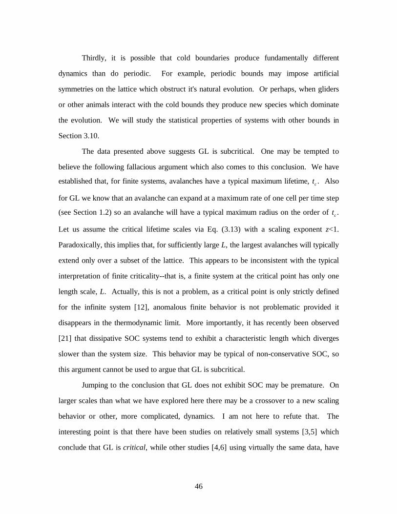
Thirdly, it is possible that cold boundaries produce fundamentally different
dynamics than do periodic. For example, periodic bounds may impose artificial
symmetries on the lattice which obstruct it's natural evolution. Or perhaps, when gliders
or other animals interact with the cold bounds they produce new species which dominate
the evolution. We will study the statistical properties of systems with other bounds in
Section 3.10.
The data presented above suggests GL is subcritical. One may be tempted to
believe the following fallacious argument which also comes to this conclusion. We have
established that, for finite systems, avalanches have a typical maximum lifetime, tc. Also
for GL we know that an avalanche can expand at a maximum rate of one cell per time step
(see Section 1.2) so an avalanche will have a typical maximum radius on the order of tc.
Let us assume the critical lifetime scales via Eq. (3.13) with a scaling exponent z<1.
Paradoxically, this implies that, for sufficiently large L, the largest avalanches will typically
extend only over a subset of the lattice. This appears to be inconsistent with the typical
interpretation of finite criticality--that is, a finite system at the critical point has only one
length scale, L. Actually, this is not a problem, as a critical point is only strictly defined
for the infinite system [12], anomalous finite behavior is not problematic provided it
disappears in the thermodynamic limit. More importantly, it has recently been observed
[21] that dissipative SOC systems tend to exhibit a characteristic length which diverges
slower than the system size. This behavior may be typical of non-conservative SOC, so
this argument cannot be used to argue that GL is subcritical.
Jumping to the conclusion that GL does not exhibit SOC may be premature. On
larger scales than what we have explored here there may be a crossover to a new scaling
behavior or other, more complicated, dynamics. I am not here to refute that. The
interesting point is that there have been studies on relatively small systems [3,5] which
conclude that GL is critical, while other studies [4,6] using virtually the same data, have
46

concluded that GL is subcritical. These latter arguments have been made on the basis of
the average lifetime of the avalanches (also called average decay time).
3.7. Average decay time
If GL is critical then, in the thermodynamic limit, the average lifetime of the avalanches
should diverge. For finite lattices it must scale as tcb2+ as we see if we consider the change
of variables u t tc= in
t t f t t dt
t u f u du
t
bc
cb b
cb
∝
∝
∝
+∞
+ +∞
+
∫
∫
1
0
2 1
0
2
( )
( ) . (3.14)
Knowing how the critical lifetime scales with the system size (Eq. (3.13), valid for
small L) we can predict how the average decay time should scale:
t t
L
cb
z b
∝
∝
+
+
2
2( )(3.15)
where, from Figures 3.7 and 3.10, z b( ) . .2 0 223 0 012+ = ± . Using this value, we
compare the predicted scaling of the average decay time with our data. The results,
shown below, seem to indicate that <t> does not scale as expected but seems to plateau at
t = ±165 6 , validating the results for the critical lifetime. This stabilization was also
observed by Bennett and Bourzutschky [4] at roughly the same value of L ≈ 181. They
studied square, periodic lattices up to 1024 1024× lattices and observed no further
increase in the average decay time on these scales.
Only a subset of the average decay time data fits fairly well to the predicted power
law. The first point (L=64) does not fit because this run suffered from extreme
corrections to scaling -- it did not satisfy Eq. (3.14). The last point (L=256) also does not
fit the predicted scaling law. In this case, however, we understand this as resulting
47

directly from the informtion in Figure 3.10. This suggests the method of using average
decay time as a predictor in scaling analyses is valid, and the results here indicate that GL
is subcritical (because the largest lattice does not fit the expected scaling law).
70
80
90
100
200
32 64 128 256 512
aver
age
lifet
ime,
<t>
system size, L
Figure 3.11: Average lifetime as a function of system size for periodic lattices.
The predicted scaling exponent, 0 223 0 012. .± , (line) fits a subset of the actual
data (points).
3.7.1. Other moments of the distribution
Some researchers [4,6] believe this represents clear proof that GL must be subcritical.
Alstrøm and Leão [5] offer an alternative explanation: they suggest that the discreteness of
small avalanches pollutes the estimation of the average decay time, making it unreliable.
The reader will recall that when we first calculated the critical exponents, we explicitly
ignored data from small avalanches because of fluctuations caused by the lattice's discrete
nature. (These data points were included in our second attempt, however.) Alstrøm and
Leão suggest higher moments, which favour large avalanches, would minimize the
48

disturbances caused by the small avalanches and produce fits in agreement with finite-
scaling predictions, thus reasserting that GL is critical. (They did not actually include this
analysis in their paper, but merely outlined the procedure.)
In parallel with Eq. (3.14) the µ 'th moment of the distribution of lifetimes should
scale like
t t
L
cb
z b
µ µ
µ
∝
∝
+ +
+ +
1
1( ). (3.16)
We would like to compare this predicted scaling with that determined directly from the
data. A convergence of these values for larger moments would suggest, in agreement with
Alstrøm and Leão's prediction, that the discrepancy observed in Figure 3.11 is due to the
low end of the distribution. However, if the values diverge for larger moments, then the
discrepancy is due to the high end above the critical lifetime. Calculating the moments for
periodic lattices of various dimensions and fitting them to a finite-scaling power law I
have recovered the best fit scaling exponents and plotted them below.
49
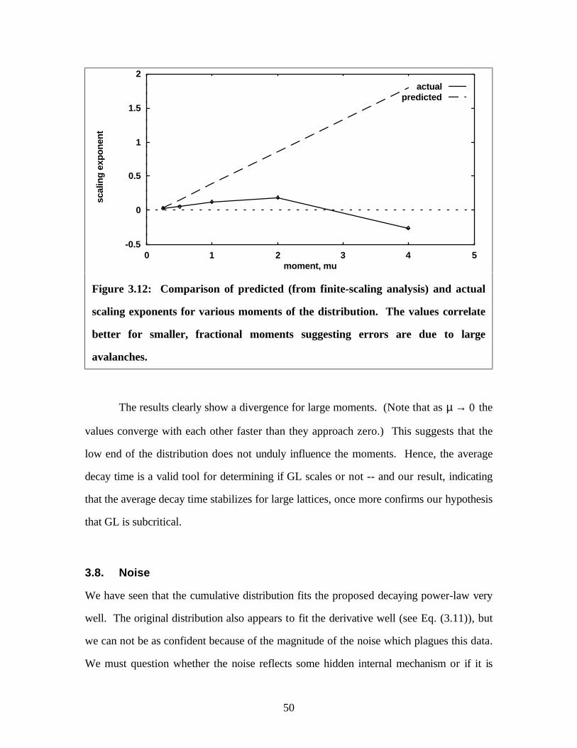
-0.5
0
0.5
1
1.5
2
0 1 2 3 4 5
scal
ing
expo
nent
moment, mu
actualpredicted
Figure 3.12: Comparison of predicted (from finite-scaling analysis) and actual
scaling exponents for various moments of the distribution. The values correlate
better for smaller, fractional moments suggesting errors are due to large
avalanches.
The results clearly show a divergence for large moments. (Note that as µ → 0 the
values converge with each other faster than they approach zero.) This suggests that the
low end of the distribution does not unduly influence the moments. Hence, the average
decay time is a valid tool for determining if GL scales or not -- and our result, indicating
that the average decay time stabilizes for large lattices, once more confirms our hypothesis
that GL is subcritical.
3.8. Noise
We have seen that the cumulative distribution fits the proposed decaying power-law very
well. The original distribution also appears to fit the derivative well (see Eq. (3.11)), but
we can not be as confident because of the magnitude of the noise which plagues this data.
We must question whether the noise reflects some hidden internal mechanism or if it is
50

simply experimental error. The easiest way to test this is by generating a synthetic data set
from the theoretical distribution, and comparing the noise levels. The synthetic data set is
generated by choosing avalanche lifetimes with the probability given in Eq. (3.11) [7, pp.
287-8]. Hence, the events are guaranteed to be independent and the noise will be
Gaussian in form (although it may not appear Gaussian on a log-log graph).
If the events (avalanches) are interdependent (suggesting a deeper analysis is
required) then we would expect the noise level to deviate from that predicted by the
synthetic data set. For example, if avalanches of similar size are positively correlated, we
may well expect the noise levels to be smaller than predicted.
Using the theoretical distribution with the parameters for the 128 128× data set, I
generated ten thousand data points (the same number as in the experimental runs), and
performed the same analysis as for the actual data. The results, shown in the figure below,
closely approximate the actual 128 128× distribution. Hence, there does not appear to be
any correlation between avalanches and the noise is due to statistical fluctuations.
51

1e-07
1e-06
1e-05
0.0001
0.001
0.01
0.1
1
1 10 100 1000 10000
dist
ribut
ion,
D(t
)
lifetime, t
1e-07
1e-06
1e-05
0.0001
0.001
0.01
0.1
1
1 10 100 1000 10000
dist
ribut
ion,
D(t
)
lifetime, t
(a) (b)
Figure 3.13: Comparison of noise levels generated by a synthetic data set (a) and
the results of the 128 128× periodic run (b). Both data sets have been binned.
The strong similarity confirms our hypothesized form of the distribution function
(curve), and suggests that avalanches are indeed independent.
Given that we now know the form of the noise, we could apply this to derive a
more precise theoretical distribution. When originally fitting the function to the
cumulative distribution I ignored the variance in the data, and treated all points as being
equally reliable. A better method would estimate the standard deviation of each data point
and include this information for a better fit. Nevertheless, considering how well the curve
fits the cumulative distribution even neglecting the deviations (see Figure 3.7), I suspect
that implementing this method would not significantly alter the model parameters.
3.9. Activity
The avalanche size can be measured by more than just lifetime. If GL is critical, any other
property which measures avalanche size should also obey a power law distribution. For
example, the total activity, defined as the number of births and deaths produced by the
avalanche (see Eq. (2.9)), should have the form
52
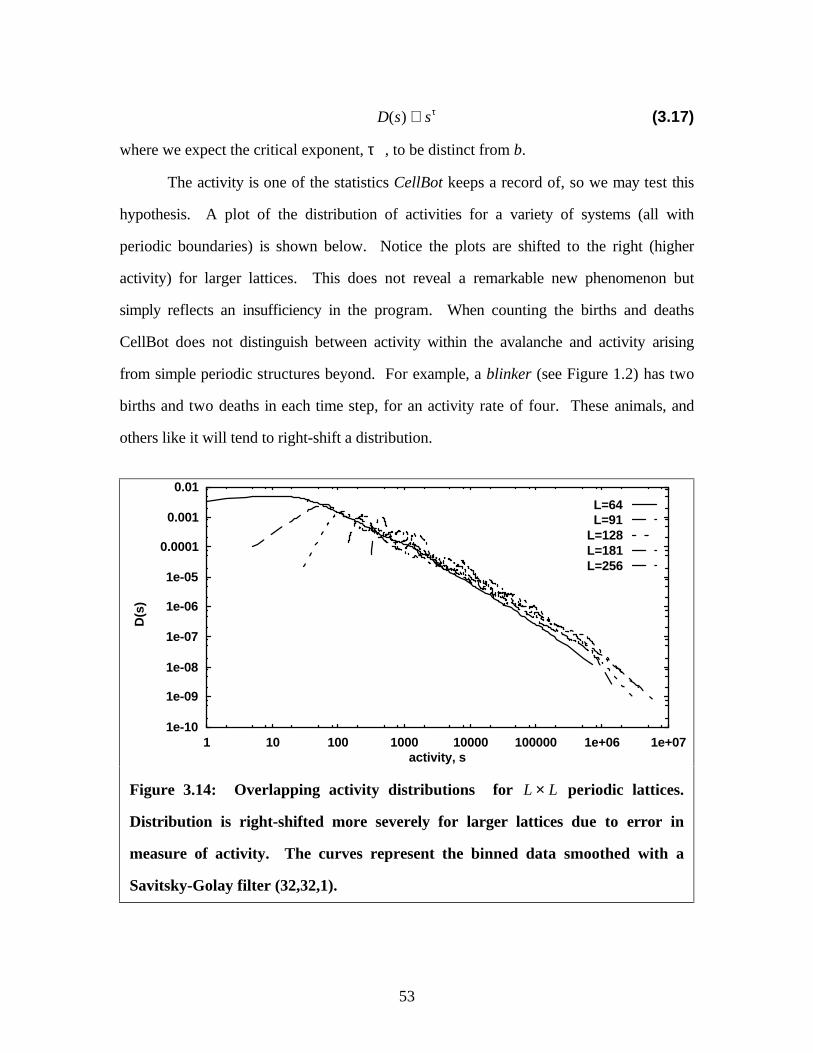
D s s( ) ∝ τ (3.17)
where we expect the critical exponent, τ , to be distinct from b.
The activity is one of the statistics CellBot keeps a record of, so we may test this
hypothesis. A plot of the distribution of activities for a variety of systems (all with
periodic boundaries) is shown below. Notice the plots are shifted to the right (higher
activity) for larger lattices. This does not reveal a remarkable new phenomenon but
simply reflects an insufficiency in the program. When counting the births and deaths
CellBot does not distinguish between activity within the avalanche and activity arising
from simple periodic structures beyond. For example, a blinker (see Figure 1.2) has two
births and two deaths in each time step, for an activity rate of four. These animals, and
others like it will tend to right-shift a distribution.
1e-10
1e-09
1e-08
1e-07
1e-06
1e-05
0.0001
0.001
0.01
1 10 100 1000 10000 100000 1e+06 1e+07
D(s
)
activity, s
L=64L=91
L=128L=181L=256
Figure 3.14: Overlapping activity distributions for L L× periodic lattices.
Distribution is right-shifted more severely for larger lattices due to error in
measure of activity. The curves represent the binned data smoothed with a
Savitsky-Golay filter (32,32,1).
53
We expect the spatial density of these species to be uniform, and hence the activity
for a lattice of dimension L will be inflated by a constant amount on the order of L2. To
correct for this error we must subtract off the estimated activity of the stable structures
from that of the avalanche. We can estimate the activity of the underlying lattice by
looking at the flip-fails, the perturbations which immediately revert to their original state
(see Section 3.2.1). In these avalanches only one count of the activity is due to the
avalanche itself, the rest represents the activity of the periodic lattice. To correct the
activity then, we must subtract the average flip-fail activity once for each time step in the
lifetime of the avalanche:
s t s t t scorrect( ) ( ) ( )= − −1 1 . (3.18)
The corrected distributions are plotted in Figure 3.15. By fitting the cumulative
distribution to a decaying power law analogous to Eq. (3.6) we recover a critical exponent
τ = − ±1 293 0 017. . , which agrees favourably with estimates from other studies: -1.4 [3]
and -1.27 [5].
54
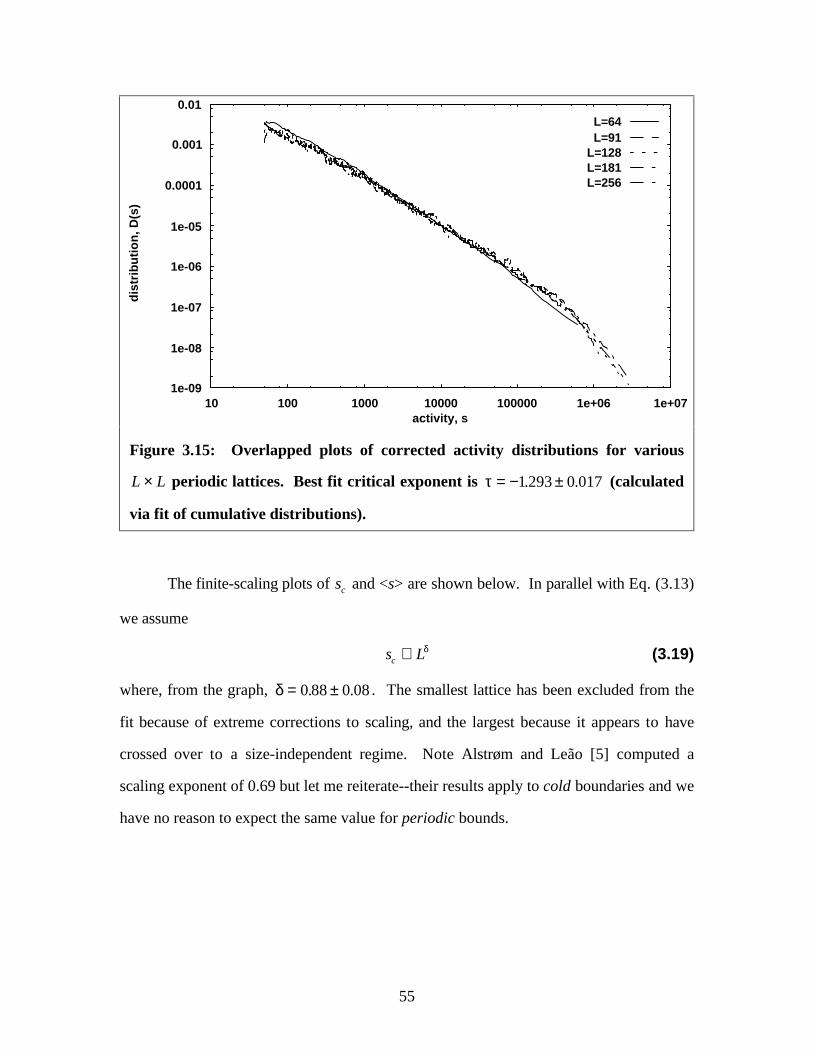
1e-09
1e-08
1e-07
1e-06
1e-05
0.0001
0.001
0.01
10 100 1000 10000 100000 1e+06 1e+07
dist
ribut
ion,
D(s
)
activity, s
L=64L=91
L=128L=181L=256
Figure 3.15: Overlapped plots of corrected activity distributions for various
L L× periodic lattices. Best fit critical exponent is τ = − ±1 293 0 017. . (calculated
via fit of cumulative distributions).
The finite-scaling plots of sc and <s> are shown below. In parallel with Eq. (3.13)
we assume
s Lc ∝ δ (3.19)
where, from the graph, δ = ±0 88 0 08. . . The smallest lattice has been excluded from the
fit because of extreme corrections to scaling, and the largest because it appears to have
crossed over to a size-independent regime. Note Alstrøm and Leão [5] computed a
scaling exponent of 0.69 but let me reiterate--their results apply to cold boundaries and we
have no reason to expect the same value for periodic bounds.
55
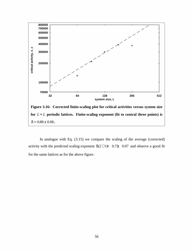
70000
100000
200000
300000
400000
500000
600000700000800000
32 64 128 256 512
criti
cal a
ctiv
ity, s
_c
system size, L
Figure 3.16: Corrected finite-scaling plot for critical activities versus system size
for L L× periodic lattices. Finite-scaling exponent (fit to central three points) is
δ = ±0 88 0 08. . .
In analogue with Eq. (3.15) we compare the scaling of the average (corrected)
activity with the predicted scaling exponent δ τ( ) . .2 0 73 0 07+ = ± and observe a good fit
for the same lattices as for the above figure.
56

700080009000
10000
20000
30000
40000
50000
60000
70000
32 64 128 256 512
aver
age
activ
ity, <
s>
system size, L
Figure 3.17: Average corrected activity as a function of system size for L L×
periodic lattices. The predicted scaling exponent, 0 73 0 07. .± , fits a subset of the
data fairly well.
3.10. Boundary conditions
It has been suggested that the debate over GL's criticality is a result of applying different
boundary conditions. In the thermodynamic limit we expect boundary effects to
disappear, but they may have important consequences in finite lattices. Bak, et al. [3] and
Alstrøm and Leão [5] applied cold (also called open) boundaries and they both concluded
GL is critical. Bennett and Bourzutschky [4] reached opposite conclusions using periodic
boundaries. Later, though, Hemmingsson [6] also concluded GL was subcritical, but he
used cold boundaries. Note the general shape of all distributions shown in these
references are similar to those shown above in Figures 3.6 and 3.15. I see no evidence in
any of these papers that the type of boundaries affect the dynamics significantly.
Nevertheless, I would be negligent if I did not explore the possibility for myself.
57
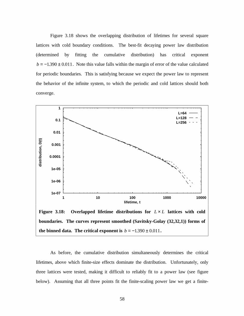
Figure 3.18 shows the overlapping distribution of lifetimes for several square
lattices with cold boundary conditions. The best-fit decaying power law distribution
(determined by fitting the cumulative distribution) has critical exponent
b = − ±1390 0 011. . . Note this value falls within the margin of error of the value calculated
for periodic boundaries. This is satisfying because we expect the power law to represent
the behavior of the infinite system, to which the periodic and cold lattices should both
converge.
1e-07
1e-06
1e-05
0.0001
0.001
0.01
0.1
1
1 10 100 1000 10000
dist
ribut
ion,
D(t
)
lifetime, t
L=64L=128L=256
Figure 3.18: Overlapped lifetime distributions for L L× lattices with cold
boundaries. The curves represent smoothed (Savitsky-Golay (32,32,1)) forms of
the binned data. The critical exponent is b = − ±1390 0 011. . .
As before, the cumulative distribution simultaneously determines the critical
lifetimes, above which finite-size effects dominate the distribution. Unfortunately, only
three lattices were tested, making it difficult to reliably fit to a power law (see figure
below). Assuming that all three points fit the finite-scaling power law we get a finite-
58

scaling exponent of 0.54. This agrees very nicely with Alstrøm and Leão's estimate of
0.52 [5] using lattices up to L=1024.
300
400
500
600
700800900
1000
2000
32 64 128 256 512
criti
cal l
ifetim
e, t_
c
system size, L
Figure 3.19: Finite-scaling plot of critical lifetimes for L L× lattices with cold
boundaries. The scaling exponent is estimated at z = ±0 54 0 09. . .
If we again plot the average lifetime against system size (below), we observe a
good fit to the theoretical result. The only qualitative difference between the cold
boundaries and periodic boundaries is that we do not observe any stabilization in the
critical lifetime or the average decay time for large lattices.
59
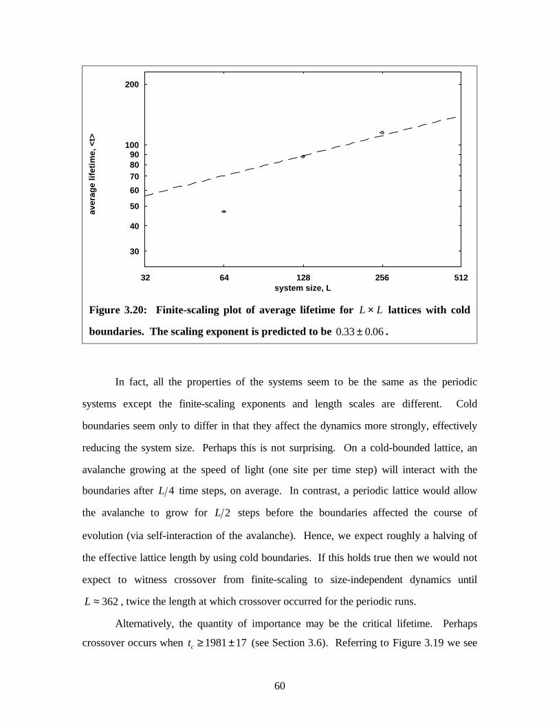
30
40
50
60
708090
100
200
32 64 128 256 512
aver
age
lifet
ime,
<t>
system size, L
Figure 3.20: Finite-scaling plot of average lifetime for L L× lattices with cold
boundaries. The scaling exponent is predicted to be 0 33 0 06. .± .
In fact, all the properties of the systems seem to be the same as the periodic
systems except the finite-scaling exponents and length scales are different. Cold
boundaries seem only to differ in that they affect the dynamics more strongly, effectively
reducing the system size. Perhaps this is not surprising. On a cold-bounded lattice, an
avalanche growing at the speed of light (one site per time step) will interact with the
boundaries after L 4 time steps, on average. In contrast, a periodic lattice would allow
the avalanche to grow for L 2 steps before the boundaries affected the course of
evolution (via self-interaction of the avalanche). Hence, we expect roughly a halving of
the effective lattice length by using cold boundaries. If this holds true then we would not
expect to witness crossover from finite-scaling to size-independent dynamics until
L ≈ 362, twice the length at which crossover occurred for the periodic runs.
Alternatively, the quantity of importance may be the critical lifetime. Perhaps
crossover occurs when tc ≥ ±1981 17 (see Section 3.6). Referring to Figure 3.19 we see
60

this would occur when L ≈ 612. In either case, it is not surprising that the properties
finite-scale as nicely as they do. This does not contradict our previous conclusion that GL
is subcritical, but merely indicates that we must study larger lattices before we should
expect to observe crossover into a size-independent regime.
3.11. Geometry
So far we have examined square lattices with periodic and cold boundaries. It may be
interesting and enlightening to explore some more exotic lattices. My first choice was a
strip bounded in only one dimension (with periodic boundaries). To reduce the
computational overhead I also imposed a reflective boundary across the width of the strip.
The effect is a bin like that shown in Figure 2.1(b). We define the characteristic size of the
lattice, L, as the width of the bin. The avalanche lifetime distributions for three separate
runs are shown in the figure below. Note the critical exponent (calculated by means of the
cumulative distribution), b = − ±1372 0 015. . , agrees with the two previous estimates. We
see the same drop-off for large avalanches, suggesting a finite-scaling analysis is in order.
61
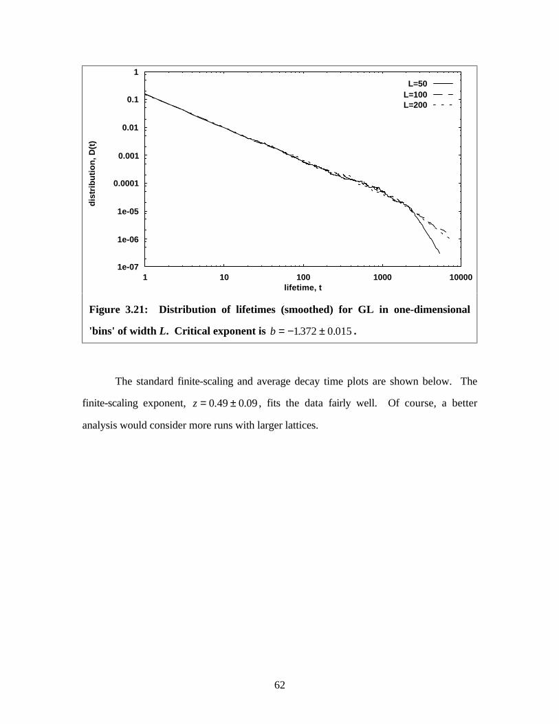
1e-07
1e-06
1e-05
0.0001
0.001
0.01
0.1
1
1 10 100 1000 10000
dist
ribut
ion,
D(t
)
lifetime, t
L=50L=100L=200
Figure 3.21: Distribution of lifetimes (smoothed) for GL in one-dimensional
'bins' of width L. Critical exponent is b = − ±1372 0 015. . .
The standard finite-scaling and average decay time plots are shown below. The
finite-scaling exponent, z = ±0 49 0 09. . , fits the data fairly well. Of course, a better
analysis would consider more runs with larger lattices.
62
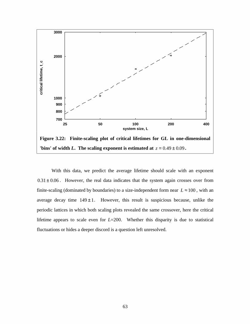
700
800
900
1000
2000
3000
25 50 100 200 400
criti
cal l
ifetim
e, t_
c
system size, L
Figure 3.22: Finite-scaling plot of critical lifetimes for GL in one-dimensional
'bins' of width L. The scaling exponent is estimated at z = ±0 49 0 09. . .
With this data, we predict the average lifetime should scale with an exponent
0 31 0 06. .± . However, the real data indicates that the system again crosses over from
finite-scaling (dominated by boundaries) to a size-independent form near L ≈ 100, with an
average decay time 149 1± . However, this result is suspicious because, unlike the
periodic lattices in which both scaling plots revealed the same crossover, here the critical
lifetime appears to scale even for L=200. Whether this disparity is due to statistical
fluctuations or hides a deeper discord is a question left unresolved.
63
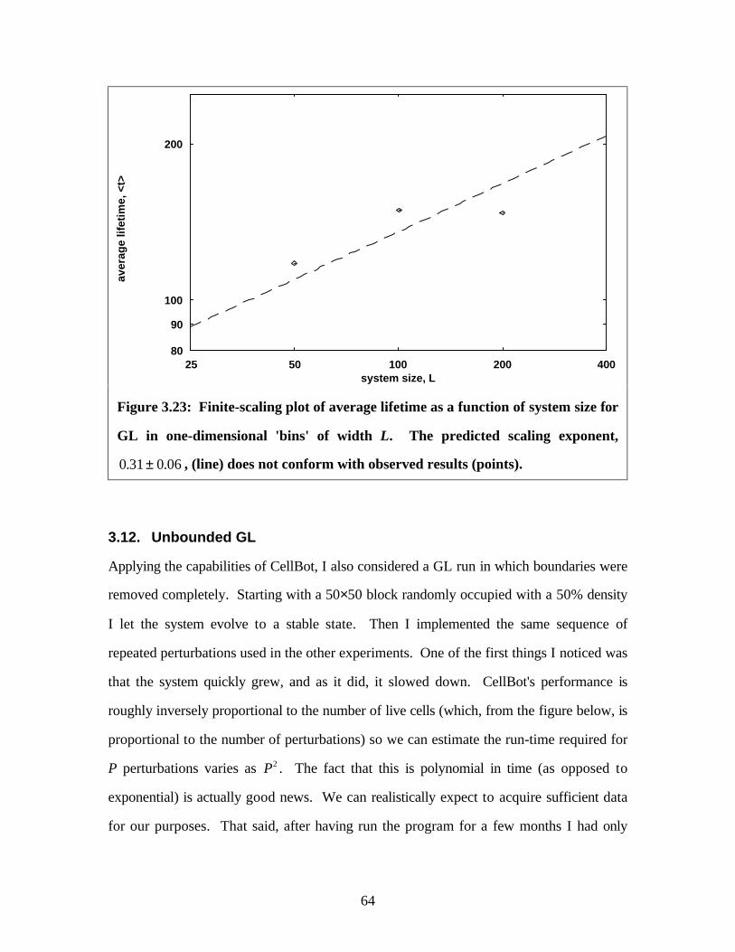
80
90
100
200
25 50 100 200 400
aver
age
lifet
ime,
<t>
system size, L
Figure 3.23: Finite-scaling plot of average lifetime as a function of system size for
GL in one-dimensional 'bins' of width L. The predicted scaling exponent,
0 31 0 06. .± , (line) does not conform with observed results (points).
3.12. Unbounded GL
Applying the capabilities of CellBot, I also considered a GL run in which boundaries were
removed completely. Starting with a 50×50 block randomly occupied with a 50% density
I let the system evolve to a stable state. Then I implemented the same sequence of
repeated perturbations used in the other experiments. One of the first things I noticed was
that the system quickly grew, and as it did, it slowed down. CellBot's performance is
roughly inversely proportional to the number of live cells (which, from the figure below, is
proportional to the number of perturbations) so we can estimate the run-time required for
P perturbations varies as P2 . The fact that this is polynomial in time (as opposed to
exponential) is actually good news. We can realistically expect to acquire sufficient data
for our purposes. That said, after having run the program for a few months I had only
64
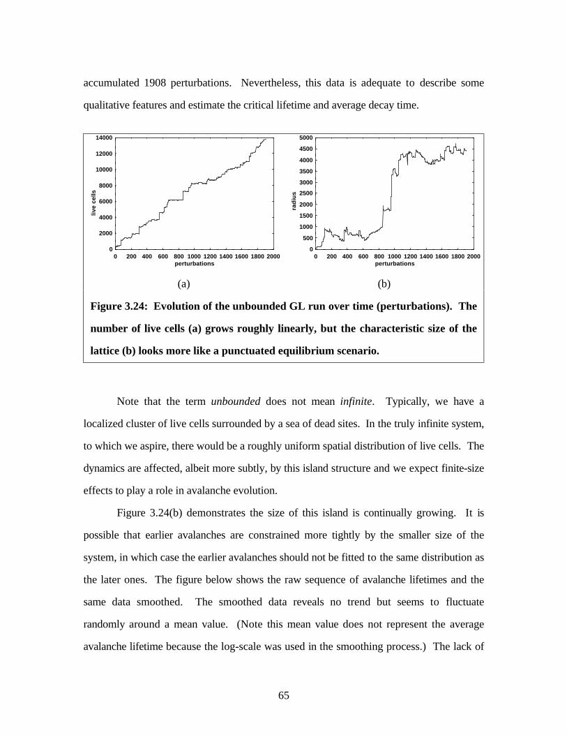
accumulated 1908 perturbations. Nevertheless, this data is adequate to describe some
qualitative features and estimate the critical lifetime and average decay time.
0
2000
4000
6000
8000
10000
12000
14000
0 200 400 600 800 1000 1200 1400 1600 1800 2000
live
cells
perturbations
0
500
1000
1500
2000
2500
3000
3500
4000
4500
5000
0 200 400 600 800 1000 1200 1400 1600 1800 2000
radi
us
perturbations
(a) (b)
Figure 3.24: Evolution of the unbounded GL run over time (perturbations). The
number of live cells (a) grows roughly linearly, but the characteristic size of the
lattice (b) looks more like a punctuated equilibrium scenario.
Note that the term unbounded does not mean infinite. Typically, we have a
localized cluster of live cells surrounded by a sea of dead sites. In the truly infinite system,
to which we aspire, there would be a roughly uniform spatial distribution of live cells. The
dynamics are affected, albeit more subtly, by this island structure and we expect finite-size
effects to play a role in avalanche evolution.
Figure 3.24(b) demonstrates the size of this island is continually growing. It is
possible that earlier avalanches are constrained more tightly by the smaller size of the
system, in which case the earlier avalanches should not be fitted to the same distribution as
the later ones. The figure below shows the raw sequence of avalanche lifetimes and the
same data smoothed. The smoothed data reveals no trend but seems to fluctuate
randomly around a mean value. (Note this mean value does not represent the average
avalanche lifetime because the log-scale was used in the smoothing process.) The lack of
65
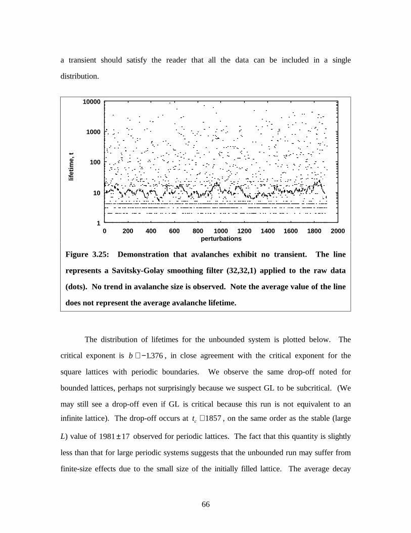
a transient should satisfy the reader that all the data can be included in a single
distribution.
1
10
100
1000
10000
0 200 400 600 800 1000 1200 1400 1600 1800 2000
lifet
ime,
t
perturbations
Figure 3.25: Demonstration that avalanches exhibit no transient. The line
represents a Savitsky-Golay smoothing filter (32,32,1) applied to the raw data
(dots). No trend in avalanche size is observed. Note the average value of the line
does not represent the average avalanche lifetime.
The distribution of lifetimes for the unbounded system is plotted below. The
critical exponent is b ≅ −1376. , in close agreement with the critical exponent for the
square lattices with periodic boundaries. We observe the same drop-off noted for
bounded lattices, perhaps not surprisingly because we suspect GL to be subcritical. (We
may still see a drop-off even if GL is critical because this run is not equivalent to an
infinite lattice). The drop-off occurs at tc ≅ 1857 , on the same order as the stable (large
L) value of 1981 17± observed for periodic lattices. The fact that this quantity is slightly
less than that for large periodic systems suggests that the unbounded run may suffer from
finite-size effects due to the small size of the initially filled lattice. The average decay
66

time, 152, being smaller than expected, also confirms that the run is inhibited by the small
initial seed. It would be interesting to study this run at later times to determine if the
critical lifetime and average decay time have increased.
1e-07
1e-06
1e-05
0.0001
0.001
0.01
0.1
1
1 10 100 1000 10000
dist
ribut
ion,
D(t
)
lifetime, t
Figure 3.26: Distribution of lifetimes for the unbounded GL. The power law fit
exponent is b ≅ −1376. . The critical lifetime is estimated at tc ≅ 1857 and the
average avalanche lifetime is t ≅ 152.
3.12.1. Gliders and the characteristic radius
Up to now I have discussed the system size without mentioning how it was measured. For
bounded lattices this is trivial, but for the unbounded system it becomes slightly more
complicated. At first guess one would simply define a bounding box which is the
minimum size to contain all live cells. Unfortunately this does not accurately represent GL
very well because, looking at Figure 3.27, we see that the unbounded system consists of
two domains: the cluster domain and the glider domain. The glider domain arises from
the central cluster periodically spitting out gliders as it evolves. Initially, these gliders,
67
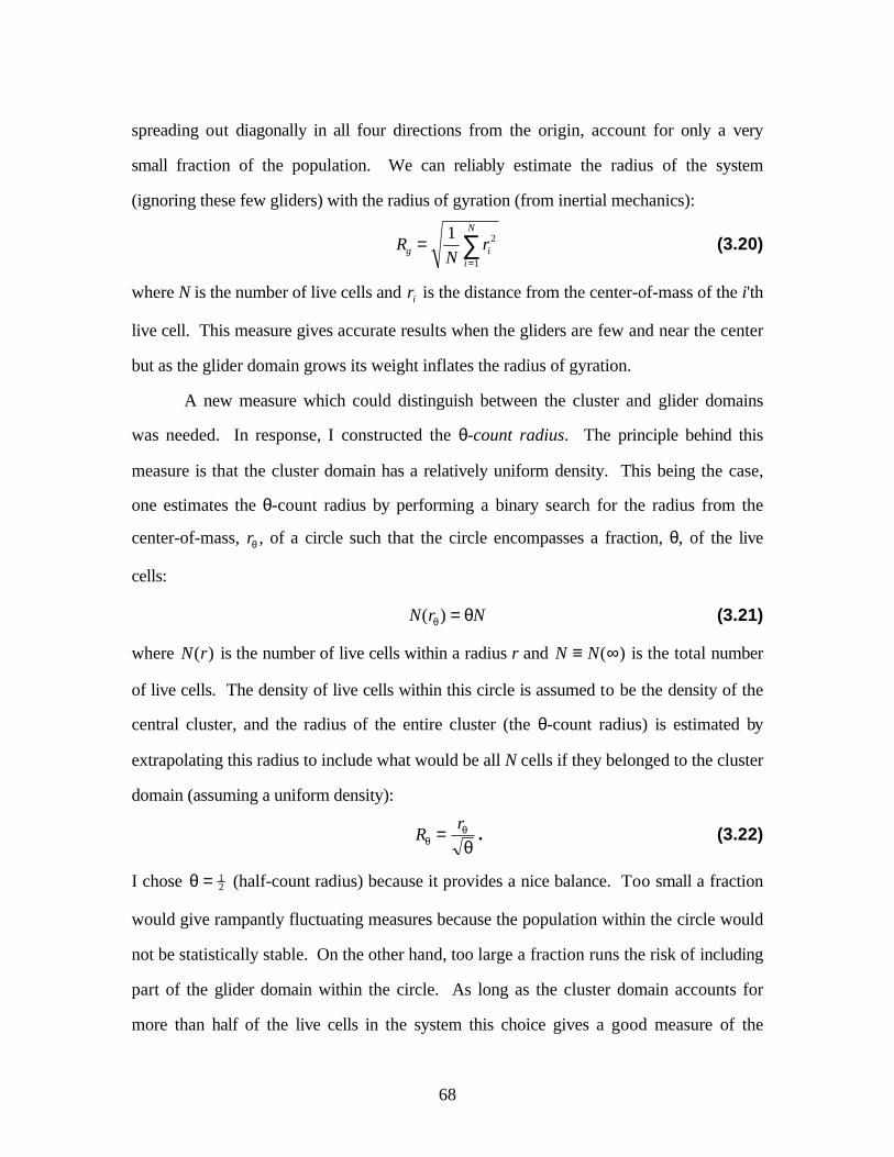
spreading out diagonally in all four directions from the origin, account for only a very
small fraction of the population. We can reliably estimate the radius of the system
(ignoring these few gliders) with the radius of gyration (from inertial mechanics):
RN
rg ii
N
==∑1 2
1
(3.20)
where N is the number of live cells and ri is the distance from the center-of-mass of the i 'th
live cell. This measure gives accurate results when the gliders are few and near the center
but as the glider domain grows its weight inflates the radius of gyration.
A new measure which could distinguish between the cluster and glider domains
was needed. In response, I constructed the θ-count radius. The principle behind this
measure is that the cluster domain has a relatively uniform density. This being the case,
one estimates the θ-count radius by performing a binary search for the radius from the
center-of-mass, rθ , of a circle such that the circle encompasses a fraction, θ, of the live
cells:
N r N( )θ θ= (3.21)
where N r( ) is the number of live cells within a radius r and N N≡ ∞( ) is the total number
of live cells. The density of live cells within this circle is assumed to be the density of the
central cluster, and the radius of the entire cluster (the θ-count radius) is estimated by
extrapolating this radius to include what would be all N cells if they belonged to the cluster
domain (assuming a uniform density):
Rr
θθ
θ= . (3.22)
I chose θ = 12 (half-count radius) because it provides a nice balance. Too small a fraction
would give rampantly fluctuating measures because the population within the circle would
not be statistically stable. On the other hand, too large a fraction runs the risk of including
part of the glider domain within the circle. As long as the cluster domain accounts for
more than half of the live cells in the system this choice gives a good measure of the
68

characteristic radius. In the figure below, the half-count radius would give an even better
estimate except that the center-of-mass is being shifted by the weight of the glider domain.
100000
-80000
-60000
-40000
-20000
0
20000
40000
60000
80000
00000
-100000-80000-60000-40000-200000 20000400006000080000100000-20000
-15000
-10000
-5000
0
5000
10000
15000
20000
-15000-10000-5000 0 5000100001500020000
-2000
-1000
0
1000
2000
3000
4000
5000
6000
-2000-1000 0 100020003000400050006000
(a) (b) (c)
Figure 3.27: Sample unbounded GL configurations. Snapshots taken at
perturbation 1906, time step 4314. The full system (a) is dominated by the glider
domain. The radius of gyration (b) and half-count radius (c) attempt to filter out
this region.
The gliders also complicate the dynamics in other ways. One important property
of SOC systems is that the driving rate approaches zero (see Section 5.2.2). This implies
that all gliders should have moved off to infinity (disappeared) before the system is
perturbed. As it stands the system is perturbed when it reaches stability, even though the
gliders are still active. The problem is that, using the perturbation method mentioned in
Section 3.2.1, it is possible that these gliders could be perturbed. In fact, as the glider
domain grows, it may become the dominant force in the evolution and accrue most of the
perturbations. I had not considered this possibility when collecting the above data. The
effect of perturbations in the glider domain is to form clusters at unnaturally large
distances from the central cluster, weighting the glider domain even more. If I had it to do
over again, I would restrict perturbations to occur within the half-count radius of the
69

center-of-mass. It is unclear whether this would significantly alter the distribution of
avalanches.
70
4. Mean-field and mixing
4.1. Introduction
We now turn our attention to another method developed for analyzing the many-body
problem. Mean-field theories have been successful in predicting critical transitions in such
systems as the Ising model--a mathematically idealized magnet [22]. The Ising model is
relevant because it shares some commonalities with GL: namely, it is consists of a
spatially-extended lattice of finite-state points which are constricted to interactions with
only nearest neighbors. Perhaps, then, a mean-field analysis would provide some insight
for us.
As the name implies, mean-field theory proceeds by replacing the particulars of an
interaction with an expectation value which represents the system as a whole. Each site is
assumed to be identical, and as such, any particular site's interactions with its neighbors
can be approximated by a mean field. Further, because this site is identical to the others,
the field is self-consistent. That is, the field represents some parameter of the neighboring
sites, and this parameter must also describe the central site itself. This last requirement
makes the transcendental problem easily solvable.
4.2. GL's mean field map
In GL, transitions are determined by the number of live cells in a neighborhood.
This suggests we use the probability of each cell being alive as our mean field. On a large
scale, this parameter is just the population density, c. Given such a field, the probability of
exactly σ live neighbors surrounding a site is given by the binomial distribution:
71

p c c c( , ) ( )σσ
σ σ= FHG
IKJ
− −81 8 . (4.1)
Of course, the central site is also going to have an occupation probability c (self-
consistency requirement). Using this information we can determine the occupation
probability in the next time step from Eq. (1.3):
c t c t p c t c t p c t( ) ( ) ( , ( )) [ ( )] ( , ( ))+ = + −=
∑1 1 32
3
σσ
. (4.2)
This form is called the mean-field map and it describes not just the local probabilities, but
the evolution of the global population. The map is plotted below in Figure 4.1, showing
the fixed points and their stabilities. These values suggest that if the system was started
from an initial population in the range c( ) ( . , . )0 0 192 0 564∈ then it will evolve to a final
population of c( ) .∞ = 0 370 . Otherwise, the system will decay and eventually disappear
altogether.
0
0.1
0.2
0.3
0.4
0.5
0.6
0 0.2 0.4 0.6 0.8 1
c(t+
1)
c(t)
Figure 4.1: Projected mean-field map for GL. Fixed points lie at 0 (stable), 0.192
(unstable) and 0.370 (stable). These results are incompatible with experimental
observations.
72

Of course, we know GL has a stable population density of roughly 0.03, in
disagreement with the predicted value of 0.370, above. One may question why mean-field
theory makes incorrect predictions for GL. By replacing particular interactions with an
average field which ignores spatial inhomogeneity we must be losing information
significant to GL's evolution. In fact, GL is dominated by spatial correlations which mean-
field theories ignore. As a GL population evolves, each of the cells strives to reach a state
compatible with its neighbors. The final, stable configuration consists of cells which are
correlated over very long distances. (If GL is critical we expect the correlation length to
diverge.)
4.3. Long-range mixing
We know mean-field theory ignores spatial correlations, and hence fails to properly
represent GL. It may be interesting to explore the effect of modifying GL in order to
destroy correlations and test the validity of this assumption. Correlations can be broken
by mixing the cells (see Section 2.1.2). We consider the simplest case of long-range
mixing via random jumps. (Other forms of mixing tend to complicate the results [17].)
We expect, in the limit of complete mixing, m→ 1, that the global dynamics
should conform with mean-field predictions.
73

Figure 4.2: Sample equilibrium configuration of GL with long-range, m=1.0
mixing on a 256 256× lattice with periodic boundaries.
Observing how GL metamorphoses from the sparse, deterministic system seen in
Figure 1.3 to the results observed above may reveal some insights into GL's nature. In
fact, GL lies at one limit point on a bifurcation diagram where m plays the role of the
bifurcation parameter. This may reveal insights into GL's critical nature. For small m, we
expect the lattice to respond like GL with occasional perturbations. Large m, on the other
hand, should have the effect of adjusting the dynamics to conform with the mean-field
map. These predictions are confirmed in the figure below. Also, we observe a phase
transition in the intermediate values of m.
74
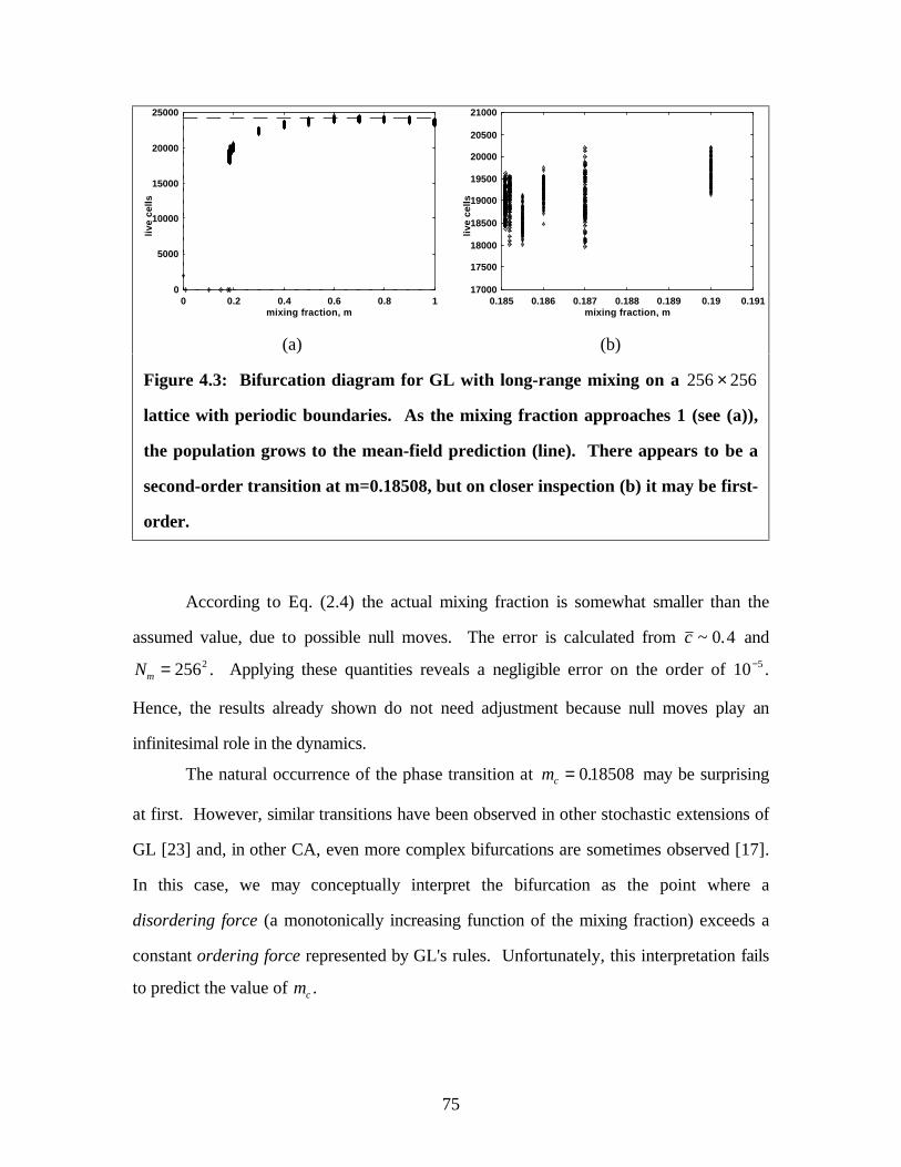
0
5000
10000
15000
20000
25000
0 0.2 0.4 0.6 0.8 1
live
cells
mixing fraction, m
17000
17500
18000
18500
19000
19500
20000
20500
21000
0.185 0.186 0.187 0.188 0.189 0.19 0.191
live
cells
mixing fraction, m
(a) (b)
Figure 4.3: Bifurcation diagram for GL with long-range mixing on a 256 256×
lattice with periodic boundaries. As the mixing fraction approaches 1 (see (a)),
the population grows to the mean-field prediction (line). There appears to be a
second-order transition at m=0.18508, but on closer inspection (b) it may be first-
order.
According to Eq. (2.4) the actual mixing fraction is somewhat smaller than the
assumed value, due to possible null moves. The error is calculated from c ~ .0 4 and
Nm = 2562. Applying these quantities reveals a negligible error on the order of 105− .
Hence, the results already shown do not need adjustment because null moves play an
infinitesimal role in the dynamics.
The natural occurrence of the phase transition at mc = 018508. may be surprising
at first. However, similar transitions have been observed in other stochastic extensions of
GL [23] and, in other CA, even more complex bifurcations are sometimes observed [17].
In this case, we may conceptually interpret the bifurcation as the point where a
disordering force (a monotonically increasing function of the mixing fraction) exceeds a
constant ordering force represented by GL's rules. Unfortunately, this interpretation fails
to predict the value of mc .
75

As mentioned above, the dynamics near the transition point seem to be defined by
the balance of the ordering and disordering subrules. It may be possible to quantify this
behavior, at least roughly. Consider a block which consists of a central site and its eight
neighbors. The first subrule attempts to correlate the block. However, if any of the cells
in the block are moved, it becomes impossible to organize. Hence, as a first
approximation, we consider mc to lie at that point such that, on average, one cell in each
block has been moved. We expect this to destroy correlations as fast as the ordering
subrule forms them. The number of cells moved in such a block is just nine times the
probability of each cell being moved. To calculate this probability we must consider the
possibility of a live cell moved out of the block (to first order this is just m) or a dead cell
being replaced by a live cell from elsewhere. This latter probability is given by
Pr( )( )
dead gets live# moves
chance of receivingcell per move
= ×−
=−
mcNc N
mc
c
mm
123
1 24 34
11
1
. (4.3)
Now, the probability of any single cell being moved is just the combination of the
probabilities for the live and dead cells respectively:
Pr( ( )Pr(cell moved) dead gets live)= + −=
mc c
mc
1
2. (4.4)
We are now in a position to estimate the critical mixing fraction. As I mentioned above,
we suspect this to occur at the point when correlations are being destroyed as fast as they
can be constructed. This suggests that, on average, one cell in each block is moved.
Since the number of cells moved is just nine times the value given in Eq. (4.4) we expect a
transition at
76

mcc =
⋅≅
1
9 20 150.
. (4.5)
We take c to be the mean-field population density because we are interested in the
equilibrium dynamics and the mean-field dynamics represent an equilibrium configuration .
This estimate agrees roughly with the observed value of 0.18508. A better estimate would
also consider the possibility that the move does not affect the transition--for example, a
neighborhood containing eight live cells would evolve in the same way regardless of
whether another cell was added or one of the eight removed. In this case correlations
could still grow, but we assume these situations are rare.
4.4. Asynchrony
In GL, correlations are set up not only spatially, but over time as well. We may expect,
then, that breaking temporal correlations should produce dynamics similar to those
observed in the last section. At first glance one may guess the figure below, which shows
a GL configuration with a low synchronisity, looks like Figure 4.2, a sample mean-field
configuration. On closer inspection, however, the reader will notice patterns of vertical
and horizontal lines which are not seen in the mean-field configuration. This supports
claims in reference [24] that asynchrony induces order in cellular automata.
77

Figure 4.4: Sample equilibrium GL configuration with asynchronous updating
(s=0.10) on a 256 256× lattice with periodic boundaries. Notice the pattern of
vertical and horizontal lines emerging.
Again, curiosity prompts us to explore the transition from GL (s=1) to asynchrony.
The figure below indicates another second-order phase transition. The dynamics
responsible for this transition and the transition observed with mixing deserve closer
inspection. For now, let me only say that we see from the graph that asynchrony is a
markedly different property than mixing and the transitions must arise from different
forces.
78

0
5000
10000
15000
20000
25000
30000
0.1 0.2 0.3 0.4 0.5 0.6 0.7 0.8 0.9 1
live
cells
synchronisity, s
Figure 4.5: Bifurcation diagram for population density as a function of
synchronisity for GL on a 256 256× periodic lattice. A second-order transition
occurs between s=0.9 and 0.95. Notice that, in the extreme, the dynamics do not
correspond to mean-field predictions (line).
79
5. Conclusions
5.1. Is GL SOC?
In this paper we have explored evidence which suggests the Game of Life (GL) is self-
organized critical (SOC) as well as evidence which suggests it is not. In an attempt to
reconcile these conflicting views we stumbled upon a tool -- a simple scaling form of the
cumulative distribution -- which clarified much of the vague and subjective evidence
supporting either claim. With this tool we were able to apply a rigorous finite-scaling
analysis and discovered that the evidence points to GL falling short of criticality.
Unfortunately, we have very little data beyond the length-scale where GL crosses over
from finite-scaling to stability -- larger lattices must be studied to confirm that GL is
subcritical.
In making the discovery that GL is subcritical we have reconciled arguments from
both camps -- we have applied a finite-scaling analysis and observed that it is in agreement
with the lack of scaling observed in the average of the distribution. We have explored a
variety of boundary conditions and alternate geometries and found no indication that these
variations affect the dynamics in any way except in the size of the lattice at which
crossover occurs. We have also discovered an unusual and perplexing scaling function in
that it increases above one before falling off to zero.
One must always constrain one's conclusions to scales which have been explored,
and hence, we will never know if GL is truly critical on all scales. The best we can say is
that GL is subcritical, at least up to such-and-such a system size.
Regardless of whether GL does exhibit SOC or not, I hope this paper conveys to
the reader the problems with the analytical tools at our disposal. New methods need to be
developed, or old methods adapted, to the exploration of spatially extended dynamical
systems far from equilibrium. In the following sections I present some of my own ideas in
the pursuit of this goal.
80

5.2. Unexplored avenues
5.2.1. Renormalization group
The renormalization group is an elegant new theory developed in the 1970s by Wilson [25,
p. 18] and others to study spatio-temporal dynamics of phenomena lacking a length-scale.
It is well suited to critical phenomena, providing a method for approximately computing
the critical exponents, and provides a conceptual framework for understanding that
enigma of criticality--universality.
The basic idea behind (real space) renormalization is that of coarse-graining,. The
lattice space of cells is partitioned into blocks of linear dimension l. Then, each block is
replaced by a single site which represents some sort of average of the block. Self-similar
properties of the transformation are exploited revealing fundamental properties of the
underlying system.
Each iteration of renormalization decreases the length scale by a magnitude l.
Hence, for systems off the critical manifold the correlation length is also rescaled,
ξ ξ→ l , pulling near-critical systems further and further from criticality (ξ = ∞) and
making them easier to analyze with traditional methods.
Unfortunately, in GL no conserved quantities have been discovered, and in
particular, there is no analogue for energy. Hence, it is impossible to construct a
Hamiltonian (the preferred quantity to obey self-similar scaling). Nevertheless, despite my
abysmal understanding of the subject, intuition tells me a renormalization approach would
go far in the deciphering of GL's mysteries.
5.2.2. Mapping onto criticality
Recently, Sornette et al [26] have described a method of mapping specific SOC models
onto dynamical critical phenomena. SOC is viewed as a result of tuning the order
81

parameter (instead of the control parameter) to approach a vanishingly small non-zero
value, which has the effect of forcing the control parameter to the critical point (see Figure
1.4(b)). Mapping SOC onto criticality has the advantage of not requiring any
conservation laws and it explains the very slow driving rate observed in all SOC systems.
In their paper Sornette et al give an example of how this mapping is implemented
on the canonical SOC model--the sandpile. They consider a physical system of a drum
containing sand which is rotated at a rate ddtθ . The rotation is driven by a torque, T. At
some critical torque, Tc , avalanches of all sizes are observed in the sand with a decaying
power law frequency. This suggests the system is at a critical point. Below this point the
torque is insufficient to rotate the drum, while above this point a non-zero average
rotation rate, ddtθ , is observed. SOC is seen as controlling the order parameter, ddt
θ ,
instead of the control parameter, T. If we require ddtθ → +0 then we incidentally force
T Tc→ , the critical value. The important point here is that there is no manual tuning of
any parameters, the critical point is found automatically.
One could explore GL in these terms. As we will see, the dynamics are driven by
site perturbations which occur only after very long times (after the system has stabilized).
This suggests, in analogy with the sandpile mapping, that the perturbation rate plays the
role of the order parameter. However, the question of what plays the role of control
parameter comes to light. I can find no clear way of interpreting GL as a critical system,
in this manner.
On a different tack, GL is suspected to be SOC because of the apparent power law
behavior observed. No experiments have been done which place GL at a critical point on
a bifurcation diagram. The problem has been finding a suitable control parameter which is
continuous and yet describes GL for some value. GL has a discrete neighborhood,
discrete rules, and a discrete alphabet (dead or alive), making it difficult to parameterize.
One method is to consider the rule space of probabilistic CA of which GL is a member.
For GL we determine the transition probabilities from Eq. (1.3):
82

p
p
0 1
1 1
0
1
→
→
=
=
GL
GL
rule
rule
( ) ( , )
( ) ( , )
σ σ
σ σ(5.1)
and
p p
p p
0 0 0 1
1 0 1 1
1
1
→ →
→ →
= −
= −
GL GL
GL GL
( ) ( )
( ) ( )
σ σ
σ σ. (5.2)
Now we construct a two-parameter family of rules which includes GL.
σ µ σ µ σ
µµ µ
µ µµ µ
p p0 1 1 1 1 2
2
1 2
1 2
1 2
0 0 0
1 0 0
2 0 1 1
3 1 1 1
4 0 0
5 0 0
→ →
−− −
− +
+
( , ) ( , )
max( , )
max( , ) min( , )
min( , )
max( , ) max( , )
(5.3)
for µ µ1 2 1 1, ( , )∈ − . The other probabilities are exclusive as in Eq. (5.2). Upon close
examination we observe that GL corresponds to ( , ) ( , )µ µ1 2 0 0= . Physically, the above
table can be interpreted as meaning that the CA prefers a more heavily occupied
neighborhood for larger values of the parameters and a sparser neighborhood for smaller
values. The parameters are responsible for shifting the location of the crest in Eq. (5.3).
It is unclear whether this method will give any meaningful results but I intend to
study it in the future. I foresee difficulties, however, because GL differs in one crucial
way from the CA nearby in the parameter-space: it is deterministic. Hence, it may set up
long-range correlations and large-scale structures which probabilistic systems tend to
smear out. We have already seen examples of this when we studied mixing and
asynchrony in Chapter 4.
5.2.3. Directed Percolation
To study the dynamics in GL we considered the effect of a single site perturbation--
flipping the state of a cell and watching the resulting avalanche. Statistically speaking, the
83

avalanche has a chance of either growing or shrinking at each time step, as it evolves.
Perhaps this evolution can be interpreted in terms of a directed percolation problem.
Directed percolation [27] is used to model the flow of fluid through a porous
material. At each time step the fluid can penetrate further into the material with some
probability, p. If we consider the family of all such models, then we observe a critical
transition as p increases past some probability pc . For small p, the fluid penetration is
inevitably halted, eventually. Above pc , however, there will always be at least one path
which permeates the entire length of the substance. The value of pc depends on the
dimensionality, geometry, et cetera.
It is possible that the evolution of an avalanche can be modelled in these terms. If
we can determine that GL avalanches are guaranteed the possibility of traversing the entire
lattice space, does this not put some lower bound on GL's complexity? One of GL's
sticking points, the strong correlations which extend over the lattice may not apply (in the
same way) to the avalanche as it does to the space itself. If this is true, a mean-field
theory, like directed percolation, may be applicable to the avalanches.
5.3. Summary
As can be seen, GL holds a wealth of possible future research topics. Remember, though,
we are interested in GL not for its own sake, but in order to find tools which may be
useful for the analysis of natural spatially extended dynamical systems--particularly those
near a critical point. We have seen that spatio-temporal correlations strongly affect the
dynamics of the system. Breaking these correlations, by either spatial or temporal mixing,
reduces GL's complexity and makes it more readily solvable. But natural systems with
internal chronometers do exist, and may exhibit the same complexity seen in GL.
Complexity sometimes occurs even without synchronization. In these cases, the
experience we have gained from the study of GL will be useful.
84

A. CellBot source code
CellBot copyright © Hendrik J. Blok 1994, 1995
This is the source code, in C, for the program CellBot. All files included here may
be freely copied and redistributed, without modification, provided the copyright notice is
not removed. This program is for non-commercial use only and may not be sold for
profit.
The files nr.h and ran1.c can be found in Numerical Recipes [7] and are not
included here. However, nrutil.c and nrutil.h are included because they include important
modifications to the original code (placed into the public domain by Numerical Recipes
Software). To compile CellBot simply copy all these files to the same directory and
compile them. Then link the object files to create an executable. Note: the function
main() which contains the heart of the algorithm, can be found in the file cb.c.
bounds.c/* CellBot - bounds.c
Copyright 1994,1995 Hendrik J. Blok
Routines for analyzing boundary conditions. Note that ALL systems are bounded, even btype=NONE. In fact these behave as PERIODIC systems with lengths equal to MAXINT. This is because large integers loop around to their maximal negative value (and vice versa).
Note: on DOS MAXINT=65535 while on Unix MAXINT=4294967295.
Modifications:
v2.05a Aug 12/94 - changed btype[] to a float in preparation for HOT boundaries - added Hot boundaries
v2.04a Aug 11/94 - in initbounds() btype is now read as a string instead of a coded integer
v2.02a Aug 10/94 - added routine initbounds() which reads boundary info. from config. file
v2.01a Aug 9/94 - changed boundary type REFLECT to REFLECT_EVEN and REFLECT_ODD
v2.00e Aug 9/94 - deleted routine single_applybounds(). Now always uses applyboundaries() for consistency. - reactivated map_inbounds() under the new name map_across(). v2.00d Aug 9/94 - in apply_boundaries() changed PERIODIC & REFLECT routines to only duplicate cells within range of border (see isonborder). v2.00c Aug 8/94 - fixed bug in how REFLECT handled corners. (It didn't!) Required complete rewrite of subroutine in applyboundaries(). - deleted map_cell(). No longer used. - temporarily disabled map_inbounds() and single_applybounds(). v2.00a July 21/94 - now can handle separate conditions for each boundary. Corner disputes are handled by choosing priorities for boundaries.*/
#include <stdlib.h> /* defines abs() */#include <string.h> /* defines stricmp() */#include "bounds.h" /* defines NONE, COLD, PERIODIC, REFLECT_EVEN, REFLECT_ODD, LOOP_OVER_BOUND(), inbounds()
*/
85
/* includes stdio.h ==> defines FILE */#include "cb.h" /* defines LOOP_OVER_CELLS(), LOOP_OVER_FLIP_NBRS() */#include "rules.h" /* defines dim, live(), maxnbrs, nbrx */#include "nrutil.h" /* defines ivector(), free_ivector(), ivector_cmp(), CMP_LESS, CMP_GREATER */#include "fileio.h" /* defines fstrip() */#include "pandora.h" /* defines runtime_err() */#include "rrandom.h" /* defines flip() */
int *minx, *maxx; /* boundaries */float *btype; /* array of boundary types (by descending priority) */int *bcode; /* array of boundaries (") */
int beyondbound(int bc, int *x)/* Tests if x is outside a particular boundary. bt is of the form indicated in the configuration file.
Note: this routine ignores the possibility that btype==NONE.*/{ if (bc<0) /* minx */ if (x[-bc] < minx[-bc]) return 1; else return 0; else /* maxx */ if (x[bc] > maxx[bc]) return 1; else return 0;}
int inbounds(int *x)/* Tests whether x is within [minx..maxx]. Always returns TRUE if no boundaries.
Modifications:
v2.00a July 21/94 - now compatible with multiple boundary conditions*/{ int p;
/* check boundaries (by priority) */ for (p=1; p<= 2*dim; p++) if (beyondbound(bcode[p], x)) if (btype[p] == NONE) return 1; else return 0;
/* else (is inside all bounds) */ return 1;}
void map_across(int bc, float bt, int *x)/* Maps x across the boundary bc according to the boundary type, bt.
Modifications:
v2.05a Aug 12/94 - changed switch() to if..else because switch doesn't accept floats
v2.01a Aug 9/94 - added support for REFLECT_EVEN and REFLECT_ODD
v2.00e Aug 9/94 - renamed from map_inbounds() to map_across() - flipped boundary which PERIODIC maps across to reflect new use of routine (now designed to map in-bounds cells to out-of-bounds).*/{ if (bt==PERIODIC) { if (bc<0) x[-bc] = minx[-bc] - (maxx[-bc] - x[-bc]) -1; else x[+bc] = maxx[+bc] + (x[+bc] - minx[+bc]) +1; } else if (bt==REFLECT_EVEN) { if (bc<0) x[-bc] = minx[-bc] - (x[-bc] - minx[-bc]) -1; else x[+bc] = maxx[+bc] + (maxx[+bc] - x[+bc]) +1; } else if (bt==REFLECT_ODD) { if (bc<0) x[-bc] = minx[-bc] - (x[-bc] - minx[-bc]); else x[+bc] = maxx[+bc] + (maxx[+bc] - x[+bc]); }}
int pri_beyondbound(int p, int *x)/* Tests if x is outside a particular boundary. b is of the form indicated in the configuration file. If beyond a higher priority border or not beyond border b then returns 0. Else returns 1.
Note: you can't choose the boundary like you can in beyondbound() because if you choose one other than b[p] then it may be a higher priority boundary in which case this routine could return a false 0.
Note: this routine ignores the possibility that btype==NONE.*/{ int i;
for (i=1; i<p; i++) if (beyondbound(bcode[i], x)) return 0;
86
/* else */ if (beyondbound(bcode[p], x)) return 1; /* else */ return 0;}
int is_on_border(int *x)/* Assumes x is out-of-bounds. Returns 1 if x is a neighbor to an in-bounds cell, else returns 0.*/{ int temp = 0; int *nx = ivector(1,dim);
LOOP_OVER_FLIP_NBRS(x,nx) if (inbounds(nx)) temp = 1; }
free_ivector(nx,1,dim); return temp;}
void applyboundaries(void)/* Modifies cell states on border to reflect boundary conditions. Deals with each edge separately handling corners according to the priorities of the boundaries.
Modifications:
v2.05a Aug 12/94 - changed switch() to if..else because switch() doesn't work on floats - added Hot boundaries*/{ int p; cell *c, *like; int *x = ivector(1,dim);
for (p=2*dim; p>=1; p--) {
if (btype[p]==COLD) { LOOP_OVER_CELLS(c) if (pri_beyondbound(p,c->x)) delete_cell(&c); }
} else if (btype[p]==PERIODIC || btype[p]==REFLECT_ODD || btype[p]==REFLECT_EVEN) { /* These types map cells across boundaries. They set out- of-bounds cells to mimic the state of the corresponding in-bounds (sort of) cell.
This bit has been entirely rewritten in v2.00c. */ LOOP_OVER_CELLS(c) if (live(c) && !pri_beyondbound(p,c->x)) {
/* map c->x to out-of-bounds equivalent (x) */ ivector_cpy(x,c->x,1,dim); map_across(bcode[p], btype[p], x);
/* if just outside boundary then duplicate c */ if (pri_beyondbound(p,x) && is_on_border(x)) { like = getcell(x); like->state = c->state; } } } } else if (btype[p]>=0.0 && btype[p]<=1.0) { /* HOT */ int *outx = ivector(1,dim);
LOOP_OVER_BOUND(bcode[p], x) LOOP_OVER_NBRS(x,outx) if (pri_beyondbound(p,outx)) { c = getcell(outx); c->state = flip(btype[p]) ? x_flipstate(deadstate) : deadstate; } } } free_ivector(outx,1,dim); } } free_ivector(x,1,dim);}
void initbounds(FILE *f)/* Read boundary information from f (configuration file). Reads bcode, x, and btype.
Modifications:
v2.06a Aug 21/94 - error trapping
v2.05a Aug 12/94 - read HOT boundaries
v2.04a Aug 11/94 - btype is now entered as a string instead of a coded integer
v2.02a Aug 10/94 - initial version
87

*/{ int p; char bs[20];
/* allocate arrays */ minx = ivector(1,dim); maxx = ivector(1,dim); bcode = ivector(1,2*dim); btype = vector(1,2*dim);
for (p=1; p<=2*dim; p++) { /* read bcode */ fscanf(f, "%i", bcode+p); fstrip(f); if (bcode[p]==0 || abs(bcode[p]) > dim) runtime_err("Configuration File: bcode must be in the range +/-1 ... +/-dim");
/* read minx/maxx */ if (bcode[p] < 0) { fscanf(f, "%i", minx - bcode[p]); fstrip(f); } else { fscanf(f, "%i", maxx + bcode[p]); fstrip(f); }
/* read btype */ fscanf(f, "%s", bs); fstrip(f);
if (stricmp("None",bs)==0) btype[p] = NONE; else if (stricmp("Cold",bs)==0) btype[p] = COLD; else if (stricmp("Periodic",bs)==0) btype[p] = PERIODIC; else if (stricmp("Reflect_Odd",bs)==0) btype[p] = REFLECT_ODD; else if (stricmp("Reflect_Even",bs)==0) btype[p] = REFLECT_EVEN; else if (stricmp("Hot",bs)==0) { /* next no. is temperature */ /*
Note: COLD==0.0 so applybounds() will use COLD (erase out- of-bounds cells) if this number is 0.0 */ fscanf(f, "%f", btype+p); fstrip(f); if (btype[p]<0.0 || btype[p]>1.0) runtime_err("Configuration File: Hot boundaries must be in the range 0.0 ... 1.0"); } else runtime_err("Configuration File: boundary type not recognized"); }
for (p=1; p<=dim; p++) if (minx[p]>maxx[p]) runtime_err("Configuration File: maxx must be >= minx");}
/* turn off "'____' declared but never used" warning */#pragma warn -use•
bounds.h/*
CellBot - bounds.h
Copyright 1994,1995 Hendrik J. Blok
Modifications:
v2.14a Jun 18/95- #include stdio.h so that FILE is defined in rules.c
v2.05a Aug 12/94- changed boundary types to floats in preparation for HOT boundaries
v2.01a Aug 9/94- changed boundary type REFLECT to REFLECT_EVEN and REFLECT_ODD
*/
#ifndef _BOUNDS_H_#define _BOUNDS_H_
#include <stdio.h> /* defines FILE *//*#include "hash.h"*/
/* boundary types */#define NONE -1.0#define COLD 0.0#define PERIODIC 2.0#define REFLECT_ODD 3.0#define REFLECT_EVEN 4.0
/*The following is a control structure like the ones found in cb.h. Thisone loops over all possible x-values of a boundary.
Modifications:
v2.05a Aug 15/94- new
*/static int bndcarry;static int bndrun;#define LOOP_OVER_BOUND(b,x) ivector_cpy(x,minx,1,dim); \
if (b>0) x[b]=maxx[b]; \if (abs(b)==dim) x[dim-1]--;
\else
x[dim]--; \while (1) { \
bndcarry=1;\
for (bndrun=dim; bndrun>=1 &&bndcarry; bndrun--) { \
88

if (bndrun != abs(b)) {\
x[bndrun]++; \if
(x[bndrun] > maxx[bndrun]) { \
x[bndrun] = minx[bndrun]; \
bndcarry = 1; \} else
\
bndcarry = 0; \}
\} \if (bndcarry) break;
/* global vars. */extern float *btype; /* boundary type (by descending priority) */extern int *bcode; /* boundary code (by descending priority) */extern int *minx, *maxx; /* coordinates of boundaries */
/* function prototypes */extern int inbounds(int *x);extern void applyboundaries(void);extern void initbounds(FILE *f);
#endif /* _BOUNDS_H_ */•
cb.c/* CellBot - cb.c
Copyright 1994,1995 Hendrik J. Blok
MAIN PROGRAM
Modifications:
v2.14a Jun 18/95- in advance() mixing routine modified to work with new move_cell()
v2.13d Jun 8/95- sum count_live in fillgrid() so record_sps() works on zeroth step.
v2.13c May 19/95- now handles both DOS and Unix filename formats in configuration
file. See configure().v2.13b May 13/95
- fixed bug which halted program when t>sync*ntime. Should haltwhen sync*t>ntime.
v2.13a May 9/95- replaced t by sync*t in record_cps(), record_sps(), record_spp()
and when comparing length of last pert. Changed ntime to afloat.
v2.12a Apr 2/95- don't use random walk when mixing cells in advance()
v2.11a Mar 15/95- prevent repeat moves of each cell by flagging moved cells
v2.10a Mar 12/95- advance() now randomly mixes cells by moving some of them
v2.06a Aug 21/94 - error trapping
v2.05a Aug 12/94 - in version_cmp() now checks that input file isn't newer than the CellBot program - in fillgrid() now uses control structure LOOP_OVER_SPACE() defined in cb.h
v2.03a Aug 11/94 - added routine version_cmp() which confirms that the file being read is a recent enough version and the right type of file.
v2.02a Aug 10/94 - in configure() now swaps to initbounds() to read boundary info.
v2.00b July 27/94 - if not recovering from crash then record initial data in files (.cps & .sps)*/
/* my e-mail address */#define CB_MAILTO "[email protected]"
/*#include <stdio.h>*/#include <string.h> /* defines strlen(), strnicmp(), stricmp() */#include <stdlib.h> /* defines abs() */#include "pandora.h" /* defines runtime_err(), time_t, time() */#include "rrandom.h" /* defines flip(), rrandom(), time_t */#include "fileio.h" /* defines fexist(), fstrip(), expand_fn() */#include "bounds.h" /* defines applyboundaries(), minx, maxx, btype, inbounds() */#include "cb.h" /* defines LOOP_OVER_CELLS(), LOOP_OVER_NBRS(), LOOP_OVER_FLIP_NBRS(), LOOP_OVER_SPACE(),cell */#include "record.h" /* defines fscan_dump(), fprint_dump(), record_cps(), record_sps(), record_cpp(), record_spp() */#include "rules.h" /* defines initrules(), dim, deadstate, x_flipstate(), dead(), live(), maxnbrs, nbrx, sync, applyrules(), mixing,move_cell() */#include "stable.h" /* defines stable(), maxperiod, stablewin */
89

#include "nrutil.h" /* defines ivector(), free_ivector(), ivector_cpy(), ivector_cmp(), CMP_GREATER */
/* global variables */long nperts; /* max. # perts (nperts<0 ==> loop forever) */float ntime; /* max. # time steps on last pert */int rec_cps, /* record cells per step (boolean) */ rec_sps, /* record stats per step (boolean) */ rec_cpp, /* record cells per perturb (boolean) */ rec_spp; /* record stats per perturb (boolean) */char prefix[255]; /* prefix (path+partial filename) for all data files. */char dumpfname[255]; /* (path &) name of dumpfile */float dens; /* initial fill density within bounds */time_t dumptime; /* keeps current time, to test if dump needed */long dump_period; /* time between dumps in seconds */int delete_flag; /* used in LOOP_OVER_CELLS */int dump_flag; /* modify dumpfile? (boolean) */long count_live, /* # of live, inbounds cells */ count_activity; /* sum of changes to system over one step */long sum_activity=0; /* sum of 'count_activity' over one pert. */int *pertx; /* location of perturbation */
void main(int argc, char *argv[]){ /* function prototypes */ void configure(char cfgfname[]); void fillgrid(void); void advance(void); void addneighbors(void); void perturb(void); void notice(void);
/* variable declaration */ long pert; /* pert = 0..nperts. */ unsigned long t; /* time index */ int lastpert; /* is last pert? (boolean) */
/* copyright notice */ notice();
/* Parse command-line. */ if (argc != 2) runtime_err("Usage: CB <filename.ext>\n\n\twhere <filename.ext> is the name of the configuration file.");
/* initialize */ rrandomize(); configure(argv[1]);
/* Fill hash table. */ if (fexist(dumpfname)) fscan_dump(&pert, &t); /* read dumpfile and update pert & t */ else { fillgrid(); pert = 0; t = 0; /* If not recovering then record data. First included in v2.01a */
if (rec_cps) record_cps(pert, sync*t);if (rec_sps) record_sps(pert, sync*t);
} time(&dumptime);
/* main loop */
/* Crashes are expected to occur at applyboundaries()...advance() and at stable(). Want recordings at positions such that after recovering from a crash no info will be lost or recorded twice. Placing all suspect routines before recordings should work. With the current configuration stable() may be executed twice in a row if there is a crash. */
while (nperts < 0 || pert <= nperts) { /* nperts<0 ==> loop forever */ lastpert = (nperts >=0 && pert+1 > nperts); do { if (dump_flag && elapsed(&dumptime, (time_t) dump_period)) { fprint_dump(pert, t); }
t++;if (lastpert && sync*t > ntime) /* if last step on last pert then exit */
break;
/* H: - live cells - maybe neighbors */ applyboundaries(); /* H: - live cells - boundaries */ addneighbors(); /* H: - live cells - boundaries - neighbors */ advance(); /* H: - live cells */
if (rec_cps) record_cps(pert, sync*t);if (rec_sps) record_sps(pert, sync*t);
} while (!stable());
if (rec_cpp) record_cpp(pert);if (rec_spp) record_spp(pert,sync*t);
perturb(); /* H: - live cells - neighbors (except nbrs of pert.) */ pert++; t=0; sum_activity = 0; /* for tabulation */ }; if (dump_flag) remove(dumpfname); /* Completed execution; delete dumpfile */}
90

void configure(char cfgfname[])/* Reads all necessary information and sets up arrays, etc.
Modifications:
v2.13c May 19/95- calls expand_fn() to convert DOS<-->Unix filename formats.
Applied to argv[1], rulefname, dumpfname, and prefix.v2.13a May 9/95
- changed ntime to a float
v2.06a Aug 21/94 - error trapping
v2.02a Aug 10/94 - now uses initbounds() to read boundary info.
v2.00a July 22/94 - now reads multiple boundary conditions from configuration file (by descending priority)
v1.01a July 16/94 - dimension new variable pertx[] and initialize to 0.*/{ FILE *cfgfile; char rulefname[80]; int i;
cfgfile = fopen(expand_fn(cfgfname),"r"); if (!cfgfile) runtime_err("Configuration file not found");
version_cmp(cfgfile, "Configuration", CFG_MAJOR, CFG_MINOR);
fstrip(cfgfile); fscanf(cfgfile,"%s", rulefname); fstrip(cfgfile);
initrules(expand_fn(rulefname)); /* get dim, etc. */
initbounds(cfgfile);
/* stopping conditions */ fscanf(cfgfile,"%li", &nperts); fstrip(cfgfile);
fscanf(cfgfile,"%f", &ntime); fstrip(cfgfile);
fscanf(cfgfile,"%f", &dens); fstrip(cfgfile); if (dens<0.0 || dens>1.0) runtime_err("Configuration File: dens must be >= 0.0 and <= 1.0");
/* read maxperiod & allocate stablewin */ fscanf(cfgfile,"%i", &maxperiod); fstrip(cfgfile); if (maxperiod > 0) stablewin = (long *)lvector(0,2*maxperiod-1);
fscanf(cfgfile,"%s", dumpfname); fstrip(cfgfile);expand_fn(dumpfname);
fscanf(cfgfile,"%i", &dump_flag); fstrip(cfgfile); fscanf(cfgfile,"%li",&dump_period); fstrip(cfgfile); if (dump_period<0) runtime_err("Configuration File: dump_period must be >= 0");
fscanf(cfgfile,"%s", prefix); fstrip(cfgfile);expand_fn(prefix);
fscanf(cfgfile,"%i", &rec_cps); fstrip(cfgfile); fscanf(cfgfile,"%i", &rec_sps); fstrip(cfgfile); fscanf(cfgfile,"%i", &rec_cpp); fstrip(cfgfile); fscanf(cfgfile,"%i", &rec_spp); fstrip(cfgfile);
fclose(cfgfile);
pertx = ivector(1,dim); for (i=1; i<=dim; i++) pertx[i]=0;}
void fillgrid(void)/* Fills a fraction (dens) of cells within the boundaries to random states other than dead.
Modifications:
v2.13d Jun 8/95- tally count_live so that record_sps() works on zeroth step.
v2.05a Aug 15/94 - now uses LOOP_OVER_SPACE() defined in cb.h which loops from minx[] to maxx[]*/{ int *x = ivector(1,dim);
cell *c;
count_live=0; LOOP_OVER_SPACE(x) if (flip(dens)) { c = getcell(x); /* insert cell into hash table */
c->state = x_flipstate(deadstate); /* set state to anything but dead */count_live++; /* tally live cells
*/ } } free_ivector(x,1,dim);}
void addneighbors(void)/* Strips off all dead cells and re-adds only neighbors of live cells
91

(possibly boundaries).
Modifications:
v2.05a Aug 15/94 - caught bug: addneighbors() should LOOP_OVER_FLIP_NBRS() not LOOP_OVER_NBRS()*/{ cell *c; int *x = ivector(1,dim);
/* Delete dead cells. */ LOOP_OVER_CELLS(c) if (dead(c)) delete_cell(&c); }
/* Restore neighbors. */ LOOP_OVER_CELLS(c) if (live(c)) { LOOP_OVER_FLIP_NBRS(c->x,x) getcell(x); /* with insertions */ } } }
free_ivector(x,1,dim);}
void advance(void)/* Advance system. Assumes boundary conditions have already been applied. Also does some statistical tabulation to save time.
Operates in 2 steps: first it figures out what each the cell's new statewill be. Then it sets all current states to these values.
Modifications:
v2.14a Jun 18/95- mixing routine modified to work with new move_cell()
v2.12a Apr 2/95- no longer uses random walk but just picks new random site in
random_move().
v2.11a Mar 14/95- added support for mixflag (to prevent repeat moves) and simplified
v2.10a Mar 12/95- added mixing
*/{ cell *c, *nbr;
int *x = ivector(1,dim);int *n = ivector(0,maxnbrs);cell *newc; /* new cell allocated after move */
/* Get next state of each cell and put in c->newstate. */ LOOP_OVER_CELLS(c) if (flip(sync)) { n[0]=c->state; /* fill n[] */ LOOP_OVER_NBRS(c->x,x) nbr = ni_getcell(x);
n[nbrcount] = dead(nbr) ? deadstate : nbr->state; } c->newstate = applyrules(n); /* set c->newstate */ } else c->newstate = c->state; }
/*Move newstate to state and tabulate statistics. Also delete dead andout-of-bounds cells. Also reset mixflag in preparation for mixing.
*/ count_activity=0; count_live=0; LOOP_OVER_CELLS(c) if (inbounds(c->x)) { count_activity += abs(c->newstate - c->state); c->state = c->newstate;
if (live(c)) {count_live++;c->mixflag = 0;
} if (dead(c)) delete_cell(&c); } else delete_cell(&c); }
sum_activity += count_activity;
free_ivector(n,0,maxnbrs);
/*New to v2.10.Apply mixing rules to a cell with probability mixing. Don't moveeach cell more than once.
*/if (mixing > 0.0) {
LOOP_OVER_CELLS(c)if (flip(mixing) && c->mixflag==0) { /* mix a fraction of live cells */
newc = move_cell(c);if (newc != c) delete_cell(&c);
}}
}
free_ivector(x,1,dim);
92

}
void perturb(void)/* Perturbs a random cell in the hash table by toggling its state. We only want to toggle in-bounds cells so first delete all out-of-bounds cells.
After a crash the system will follow a different route because the index used by rrandom() will have been re-initialized. If
sync==1 and deterministic, this effect will only be noticed in perturb().
This routine does not generate the most general single-site perturbations possible. Ideally one would want to perturb ANY random site within the boundaries but this has 2 problems: (1) if there are no boundaries then how do you decide on a valid region, and (2) there would be a large number of "flip fails" (when the system immediately returns to its previous rest state) for some common rules (eg. Life). These can consume a lot of computer time, so we would like to minimize their occurence. Thus we choose the only available sites for flipping to be in the neighborhood of live cells.
Modifications:
v1.01a July 16/94 - save location of perturbation on pertx[]*/{ unsigned long countcells(void);
unsigned long p,q; cell *c;
addneighbors();
/* Delete out-of-bounds cells */ LOOP_OVER_CELLS(c) if (!inbounds(c->x)) delete_cell(&c); }
/* Perturb */ q = 1 + rrandom(countcells()); /* 1..countcells */ p=0; LOOP_OVER_CELLS(c) /* Don't use a break statement because it may */ /* not behave properly in this abstract loop. */ p++; if (p==q) { c->state=x_flipstate(c->state); ivector_cpy(pertx, c->x, 1,dim); return; } }}
unsigned long countcells(void)/* Counts the number of cells in the hash table including dead cellsand out-of-bounds cells. */{ cell *c; unsigned long i = 0;
LOOP_OVER_CELLS(c) i++; } return i;}
void notice(void)/* Copyright notice */{ printf("\n"); printf("----------------------------------------------\n"); printf("CellBot - CB - v%i.%02i%c\n", CB_MAJOR, CB_MINOR, CB_BUGFIX);
printf("Copyright 1994,1995 Hendrik J. Blok\n\n");
printf("%s\n\n", __DATE__);
printf("Send comments, suggestions and bug reports to:\n"); printf(" %s\n", CB_MAILTO); printf("----------------------------------------------\n");}
void version_cmp(FILE *f, char *ftype, int major, int minor)/* Compares first line in file with ftype, major and minor to make sure the file being read is valid. Designed to work with "Configuration" and "Rule" files.
v2.05a Aug 12/94 - now reports error if file is NEWER than CellBot program
v2.03a Aug 11/94 - new*/{ char s[255]; char errmsg[255]; char line[255]; char *lp = line; int fmajor, fminor;
fgets(line, 255, f);
/* Check for comment char. */ sprintf(errmsg, "Invalid comment character in %s File", ftype); if (lp[0] != remc)
93
runtime_err(errmsg);
/* Check for " CellBot v" */ lp++; sprintf(s, " CellBot v"); sprintf(errmsg, "Not a valid %s File", ftype); if (strnicmp(lp, s, strlen(s)) != 0) runtime_err(errmsg);
/* Read version number (assume proper format) and file type */ lp += strlen(s); sscanf(lp, "%i.%i %s", &fmajor, &fminor, s);
/* Check file type */ if (stricmp(ftype, s) != 0) runtime_err(errmsg);
/* Check version numbers */ sprintf(errmsg, "Incompatible %s File", ftype); /* is file too old? */ if (fmajor < major || (fmajor==major && fminor < minor)) runtime_err(errmsg); /* is file too new? */ if (CB_MAJOR < fmajor || (CB_MAJOR==fmajor && CB_MINOR < fminor)) runtime_err(errmsg);}
/* turn off "'___' declared but never used" warning */#pragma warn -use•
cb.h/* CellBot - cb.h
Copyright 1994,1995 Hendrik J. Blok
Modifications:
v2.14b Jun 23/95- in rules.c move_cell() doesn't change c->state and c->newstate
anymorev2.14a Jun 18/95
- in rules.c random_move() extended to handle either jumps or randomwalks. Also renamed random_move() to move_cell().
- in rules.c renamed mix_radius to mix_range
v2.13d Jun 8/95- in cb.c fixed fillgrid() so record_sps() doesn't give nulls on
zeroth step.v2.13c May 19/95
- in cb.c configure() now handles both DOS and Unix filename formatsv2.13b May 13/95
- fixed bug which prematurely halted run on last pert.v2.13a May 9/95
- time is scaled by sync so that the rate of events is conserved
v2.12a Apr 2/95- in cb.c advance() now just calls random_move() for long_range
moves (in rules.c). random_move() doesn't use random walk butrandomly picks point within distance mix_radius (in eachcoordinate).
v2.11a Mar 15/95- in cb.c prevent repeat moves of each cell when mixing in
advance() by flagging moved cells
v2.10a Mar 12/95- added mixing to advance() in cb.c. Moves a fraction of cells
to break correlations.
v2.06a Aug 21/94 - added error checking in cfg & rul file. Also checks for illegal rule case
v2.05a Aug 12/94 - in bounds.c changed btype[] to a float in preparation for HOT boundaries - in cb.c version_cmp() now checks that the input file isn't newer than the CellBot program - added new control structure LOOP_OVER_SPACE() in cb.h - added new control structure LOOP_OVER_BOUND() in bounds.h - added HOT boundaries in which the cells beyond a boundary randomly fluctuate. Note: Hot 0.0 == Cold. - in cb.c fixed bug in addneighbors() which should LOOP_OVER_FLIP_NBRS() instead of LOOP_OVER_NBRS()
v2.04a Aug 11/94 - use "Cold", "Periodic", etc. to describe boundary types in configuration file instead of integers
v2.03b Aug 11/94 - added DMP_MAJOR and DMP_MINOR to use version_cmp() in fscan_dump() v2.03a Aug 11/94 - in cb.c added routine version_cmp() which confirms that the file being read is a recent enough version and the right type of file. - added CFG_MAJOR and CFG_MINOR to use this routine in configure() - added RUL_MAJOR and RUL_MINOR to use this routine in initrules()
v2.02a Aug 10/94 - added routine initbounds() which reads boundary info. from config. file. Called by configure().
v2.01a Aug 9/94 - changed boundary type REFLECT to REFLECT_EVEN and REFLECT_ODD
94
v2.00e Aug 9/94 - in bounds.c deleted routine single_applybounds(). Now always uses applyboundaries() for consistency. - in bounds.c reactivated map_inbounds() under the new name map_across(). v2.00d Aug 9/94 - in cb.h changed LOOP_OVER_NBRS() and LOOP_OVER_FLIPNBRS() to use c->x as the first argument instead of c itself. Makes it possible to loop over the neighbors of x without allocating a cell. - used this in bounds.c to only duplicate cells if they are within range of the border. Faster, less memory. v2.00c Aug 8/94 - in bounds.c fixed bug in how REFLECT handled corners. (It didn't!) Required complete rewrite of subroutine in applyboundaries(). - in bounds.c deleted map_cell(). No longer used. - in bounds.c temporarily disabled map_inbounds() and single_applybounds(). v2.00b July 27/94 - if not recovering from crash then record initial data (.cps & .sps) v2.00a July 22/94 - now can handle separate conditions for each boundary. Corner disputes are handled by choosing priorities for boundaries.
v1.02d July 21/94 - in nrutil.c modified the vector_cmp() routines to increase speed. They now exit as soon as the criterion is met instead of looping through all elements. - changed nperts so that nperts=0 means loop through once (previously was nperts=1). v1.02c July 20/94 - in record.c modified cutoff_radius() to calculate SMALLEST radius which satisfies criteria. - in record.c added line in fprint_header() to record CellBot version number in data files. v1.02b July 19/94 - in record.c rewrote cutoff_radius(). New version is faster and simpler. v1.02a July 18/94 - in record.c added routine cutoff_radius() - in record.c eliminated double checking of live() and inbounds(). Assumes all cells in hash table are both live and in bounds. - in record.c erased routine packingdens() which assumed hash table consisted of live cells and neighbors.
v1.01a July 16/94 - added pertx[] for recording position of perturbation in .spp file - erased all duplicate #includes - added rrandomize() as seed for rrandom()
v1.00a June 19/94 - initial release*/
#ifndef _CB_H_#define _CB_H_
/* CellBot version numbers (format: #.##c) */#define CB_MAJOR 2#define CB_MINOR 14#define CB_BUGFIX 'b'
/* lowest versions of input files compatible with present version */#define CFG_MAJOR 2#define CFG_MINOR 04#define RUL_MAJOR 2#define RUL_MINOR 14#define DMP_MAJOR 1#define DMP_MINOR 00
#include <stdio.h> /* defines FILE */#include <stddef.h> /* defines NULL */#include "hash.h"
/* The following control structures are designed to make the sourcecode more readable. They must be used with caution! Nested loops are notallowed because of the reference to the global variables hashcount andnbrcount. Also, in LOOP_OVER_CELLS be very careful of how insertions anddeletions of cells are handled. Inserted cells may or may not be looped over!Finally, each structure has the opening bracket included within. Be sure not toforget the closing bracket at the end of the loop!*/static int hashcount; /* used in LOOP_OVER_CELLS */extern int delete_flag;#define LOOP_OVER_CELLS(c)
\for (hashcount=0; hashcount<HASHSIZE; hashcount++) \
for (c=H[hashcount]; c != NULL; (delete_flag ? (c=c) : (c=c->next))) { \delete_flag = 0;
/* Be sure that x is allocated with ivector() before calling LOOP_OVER_NBRS(). */static int nbrcount; /* used in LOOP_OVER_NBRS & LOOP_OVER_FLIP_NBRS */static int nbrrun;#define LOOP_OVER_NBRS(cx,x) \
for (nbrcount=1;nbrcount<=maxnbrs;nbrcount++) { \for (nbrrun=1; nbrrun<=dim; nbrrun++) \
x[nbrrun] = cx[nbrrun] + nbrx[nbrcount][nbrrun];
/* LOOP_OVER_FLIP_NBRS loops over all cells TO WHICH c IS A NEIGHBOR. Thisis NOT necessarily the same as LOOP_OVER_NBRS if the neighborhood is asymmetric. */#define LOOP_OVER_FLIP_NBRS(cx,x) \
for (nbrcount=1;nbrcount<=maxnbrs;nbrcount++) { \for (nbrrun=1; nbrrun<=dim; nbrrun++) \
x[nbrrun] = cx[nbrrun] - nbrx[nbrcount][nbrrun];
95

/* LOOP_OVER_SPACE(x) loops from x=minx to x=maxx. x must be defined before calling this structure.
Modifications:
v2.05a Aug 15/94 - new*/static int spccarry;static int spcrun;#define LOOP_OVER_SPACE(x) \
ivector_cpy(x,minx,1,dim); \x[dim]--; \while (1) { \
spccarry=1; \for (spcrun=dim; spcrun>=1 && spccarry; spcrun--) { \
x[spcrun]++; \if (x[spcrun] > maxx[spcrun]) { \
x[spcrun] = minx[spcrun]; \spccarry = 1; \
} else \spccarry = 0; \
} \if (spccarry) break;
/* global vars. */extern char prefix[255]; /* output file(s) prefix */extern char dumpfname[255]; /* name of dumpfile */extern long count_live; /* statistic: count of live cells */extern long count_activity; /* statistic: sum of changes */extern long sum_activity; /* statistic: sum of count_activity */extern int *pertx; /* location of perturbation */
/* function prototypes */extern void addneighbors(void);extern void version_cmp(FILE *f, char *ftype, int major, int minor);
#endif /* _CB_H_ */•
fileio.c/*
fileio.c
Copyright 1994,95 Hendrik J. Blok
Routines to simplify file input/output operations.*/#include <stdlib.h> /* defines getenv() */#include "fileio.h" /* includes <stdio.h> */#include "strops.h" /* includes <string.h> */
char *expand_fn(char *fn)/*
Expands filename by replacing "~" with the contents of environmentvariable home. If in MSDOS then replaces occurences of "/" with "\\"else replaces "\\" with "/".
*/{
char *home=getenv("HOME");
/* replace "~" with home (just the first occurence) */str_replace_str(fn,"~",home,1);
/* replace path separators (ie. "/" and "\\") */#ifdef __MSDOS__
str_replace_str(fn,"/","\\",-1);#else
str_replace_str(fn,"\\","/",-1);#endif /* __MSDOS__ */
return fn;}
FILE *_fopen(char *fname, char *mode)/*
Interactive file open with some error trapping.*/{
FILE *f;for (f = fopen(fname, mode); f == NULL;) {
if (strchr(mode,'w') || strchr(mode,'a') || strchr(mode,'+'))printf("Error: Unable to open output file '%s'.\nEnter new path and name: ", fname);
elseprintf("Error: Unable to find file '%s'.\nEnter new path and name: ", fname);
scanf("%s", fname);f = fopen(fname, mode);
}return f;
}
int fnextc(FILE *f)/*
Preview next character from file without skipping over it.*/{
int c;c = fgetc(f);ungetc(c, f);return(c);
}
void fstrip(FILE *f)
96

/*Strips comment lines (lines beginning with remc) from the input file.
Modifications:
May 19/95- replace fgets() with search for "\n". Don't need STRLEN anymore.
*/{
char c;while (((c = fnextc(f)) == remc) || c_in_s(c,softspaces)) {
if (c == remc) {while (c != '\n' && c != EOF) c=fgetc(f);
} else {fgetc(f);
}}
}
int _feof(FILE *f)/*
Check if end-of-file is imminent. Strips comments.*/{
fstrip(f);return(feof(f) || fnextc(f) == EOF);
}
char fnextline(FILE *f)/*
Jump to next line of input file. Returns last character read (can beused to check for end-of-file).
*/{
char c;
c=fgetc(f);while (c != '\n' && c != EOF) c=fgetc(f);return c;
}•
fileio.h/*
fileio.h
Copyright 1994,95 Hendrik J. Blok
Utilities to simplify file input/output. Designed to work under MSDOSand UNIX.
*/#ifndef _FILEIO_H_#define _FILEIO_H_
#include <stdio.h> /* defines FILE */
#define remc '#'
#ifdef __MSDOS__ /* needed for access() */#include <io.h>#define F_OK 0#define W_OK 2
#else#include <unistd.h> /* for F_OK & W_OK */
#endif
/* these use access() */#define fexist(fname) (access(fname, F_OK) == 0)#define fwritep(fname) (access(fname, W_OK) == 0)
char *expand_fn(char *);int fnextc(FILE *);void fstrip(FILE *);int _feof(FILE *);char fnextline(FILE *f);
#endif /* _FILEIO_H_ */•
hash.c/*
CellBot - hash.c
Copyright 1994 Hendrik Jan Blok
Functions for referencing and updating hash table.*/#include <stdlib.h> /* defines malloc(), free(), labs() */#include "cb.h" /* defines delete_flag, includes hash.h */#include "rules.h" /* defines dim, deadstate */#include "pandora.h" /* defines runtime_err() */#include "nrutil.h" /* defines ivector(), free_ivector(), ivector_cpy(), ivector_cmp(), CMP_EQUAL */
Hashtable_type H;
int Hash(int *x); /* prototype */
cell *getcell(int *x)/*
Returns the cell with coordinates (x,y). If cell not found then createit.
97

Modifications:
v2.11 Mar 14/95- initialize mixflag to 0
*/{
int location;cell *p;
p=ni_getcell(x);if (p!=NULL) return p;/* Else must create a new cell, initialize it, and insert it into thehash table. */p=(cell *)malloc(sizeof(cell));if (p==NULL) runtime_err("Out of memory in getcell()"); /* abort */p->x=ivector(1,dim);ivector_cpy(p->x, x, 1,dim);p->state=deadstate;p->newstate=deadstate;p->mixflag=0;location=Hash(x); /* insert in front of H[] */if (H[location] != NULL)
(H[location])->prev=p;p->next=H[location];p->prev=NULL;H[location]=p;return p;
}
cell *ni_getcell(int *x)/* Returns the cell with coordinates (x,y). If cell not found then returnNULL (no insertions). */{
int location;cell *p;
location=Hash(x);p=H[location];while (p != NULL) {
if (!ivector_cmp(p->x,x,1,dim, CMP_LESS | CMP_GREATER)) return p;else
p=p->next;}return p;
}
void delete_cell(cell **c)/* Deletes a cell from the hash table. Returns a pointer to the next cellin the hash table. */{
cell *prev, *next;int location;
prev = (*c)->prev; next = (*c)->next;
/* update links (including hash) */if (next != NULL) next->prev = prev;if (prev != NULL) prev->next = next;else { /* if prev==NULL then
set H */location = Hash((*c)->x); /* to next node
*/H[location] = next;
}
/* free memory */free_ivector((*c)->x,1,dim);free(*c);
delete_flag = 1;*c = next;
}
int Hash(int *x)/* Returns the hash-key for accessing H[]. This routine is optimized fortwo dimensions. In higher dimensions this choice may not maximize thespread or minimize collisions. */{
if (dim >= 2)return (int) (labs(x[1]+FACTOR*x[2]) % HASHSIZE);
elsereturn (int) (labs(x[1]) % HASHSIZE);
}
/* turn off "'___' declared but never used warning */#pragma warn -use•
hash.h/*
CellBot - hash.h
Copyright 1994 Hendrik Jan Blok*/
#ifndef _HASH_H_#define _HASH_H_
#define FACTOR 101#define HASHSIZE 997
typedef struct cell_tag {int state;int newstate;int mixflag; /* new in v2.11 */
98

int *x;struct cell_tag *prev, *next;
} cell;
typedef cell *Hashtable_type[HASHSIZE];
extern Hashtable_type H;
/* function prototypes */extern cell *getcell(int *x); /* with insertions */extern cell *ni_getcell(int *x); /* w/o insertions */extern void delete_cell(cell **c);
#endif /* _HASH_H_ */•
nr.h
This file can be found in Numerical Recipes [7].
nrutil.c#ifdef __TURBOC__
#include <mem.h>#endif#include <stdio.h>#include <stddef.h>#include <stdlib.h>#include "nrutil.h"#define NR_END 1#define FREE_ARG char*
/* turn off "Conversion may lose significant digits" warning */#pragma warn -sig
void nrerror(char error_text[])/* Numerical Recipes standard error handler */{
fprintf(stderr, "Numerical Recipes run-time error...\n");fprintf(stderr, "%s\n", error_text);fprintf(stderr, "...now exiting to system...\n");exit(1);
}
/***********************ALLOCATE VECTOR
***********************/
float *vector(long nl, long nh)/* allocate a float vector with subscript range v[nl..nh] */{
float *v;
v=(float *)malloc((size_t) ((nh-nl+1+NR_END)*sizeof(float)));if (!v) nrerror("allocation failure in vector()");return v-nl+NR_END;
}
int *ivector(long nl, long nh)/* allocate an int vector with subscript range v[nl..nh] */{
int *v;
v=(int *)malloc((size_t) ((nh-nl+1+NR_END)*sizeof(int)));if (!v) nrerror("allocation failure in ivector()");return v-nl+NR_END;
}
unsigned char *cvector(long nl, long nh)/* allocate an unsigned char vector with subscript range v[nl..nh] */{
unsigned char *v;
v=(unsigned char *)malloc((size_t) ((nh-nl+1+NR_END)*sizeof(unsigned char)));if (!v) nrerror("allocation failure in cvector()");return v-nl+NR_END;
}
unsigned long *lvector(long nl, long nh)/* allocate an unsigned long vector with subscript range v[nl..nh] */{
unsigned long *v;
v=(unsigned long *)malloc((size_t) ((nh-nl+1+NR_END)*sizeof(unsigned long)));if (!v) nrerror("allocation failure in lvector()");return v-nl+NR_END;
}
double *dvector(long nl, long nh)/* allocate an double vector with subscript range v[nl..nh] */{
double *v;
v=(double *)malloc((size_t) ((nh-nl+1+NR_END)*sizeof(double)));if (!v) nrerror("allocation failure in dvector()");return v-nl+NR_END;
}
fcomplex *Cvector(long nl, long nh)/* allocate a complex vector with subscript range v[nl..nh] */{
fcomplex *v;
99
v=(fcomplex *)malloc((size_t) ((nh-nl+1+NR_END)*sizeof(fcomplex)));if (!v) nrerror("allocation failure in Cvector()");return v-nl+NR_END;
}
dcomplex *dCvector(long nl, long nh)/* allocate a double complex vector with subscript range v[nl..nh] */{
dcomplex *v;
v=(dcomplex *)malloc((size_t) ((nh-nl+1+NR_END)*sizeof(dcomplex)));if (!v) nrerror("allocation failure in dCvector()");return v-nl+NR_END;
}
float **matrix(long nrl, long nrh, long ncl, long nch)/* allocate a float matrix with subscript range m[nrl..nrh][ncl..nch] */{
long i, nrow=nrh-nrl+1, ncol=nch-ncl+1;float **m;
/* allocate pointers to rows */m=(float **) malloc((size_t) ((nrow+NR_END)*sizeof(float*)));if (!m) nrerror("allocation failure 1 in matrix()");m += NR_END;m -= nrl;
/* allocate rows and set pointers to them */m[nrl]=(float *) malloc((size_t) ((nrow*ncol+NR_END)*sizeof(float)));if (!m[nrl]) nrerror("allocation failure 2 in matrix()");m[nrl] += NR_END;m[nrl] -= ncl;
for (i=nrl+1;i<=nrh;i++) m[i]=m[i-1] + ncol;
/* return pointer to array of pointers to rows */return m;
}
double **dmatrix(long nrl, long nrh, long ncl, long nch)/* allocate a double dmatrix with subscript range m[nrl..nrh][ncl..nch] */{
long i, nrow=nrh-nrl+1, ncol=nch-ncl+1;double **m;
/* allocate pointers to rows */m=(double **) malloc((size_t) ((nrow+NR_END)*sizeof(double*)));if (!m) nrerror("allocation failure 1 in dmatrix()");m += NR_END;m -= nrl;
/* allocate rows and set pointers to them */m[nrl]=(double *) malloc((size_t) ((nrow*ncol+NR_END)*sizeof(double)));if (!m[nrl]) nrerror("allocation failure 2 in dmatrix()");m[nrl] += NR_END;m[nrl] -= ncl;
for (i=nrl+1;i<=nrh;i++) m[i]=m[i-1] + ncol;
/* return pointer to array of pointers to rows */return m;
}
int **imatrix(long nrl, long nrh, long ncl, long nch)/* allocate a int imatrix with subscript range m[nrl..nrh][ncl..nch] */{
long i, nrow=nrh-nrl+1, ncol=nch-ncl+1;int **m;
/* allocate pointers to rows */m=(int **) malloc((size_t) ((nrow+NR_END)*sizeof(int*)));if (!m) nrerror("allocation failure 1 in imatrix()");m += NR_END;m -= nrl;
/* allocate rows and set pointers to them */m[nrl]=(int *) malloc((size_t) ((nrow*ncol+NR_END)*sizeof(int)));if (!m[nrl]) nrerror("allocation failure 2 in imatrix()");m[nrl] += NR_END;m[nrl] -= ncl;
for (i=nrl+1;i<=nrh;i++) m[i]=m[i-1] + ncol;
/* return pointer to array of pointers to rows */return m;
}
/* turn off "Parameter never used" warning */#pragma warn -par
float **submatrix(float **a, long oldrl, long oldrh, long oldcl, long oldch, long newrl, long newcl)/* point a submatrix [newrl..][newcl..] to a[oldrl..oldrh][oldcl..oldch] */{
long i,j, nrow=oldrh-oldrl+1, ncol=oldcl-newcl;float **m;
/* allocate array of pointers to rows */m=(float **) malloc((size_t) ((nrow+NR_END)*sizeof(float*)));if (!m) nrerror("allocation failure in submatrix()");m += NR_END;m -= newrl;
/* set pointers to rows */for (i=oldrl,j=newrl;i<=oldrh;i++,j++) m[j]=a[i]+ncol;
/* return pointer to array of pointers to rows */return m;
100
}
float **convert_matrix(float *a, long nrl, long nrh, long ncl, long nch)/* allocate a float matrix m[nrl..nrh][ncl..nch] that points to the matrixdeclared in the standard C manner as a[nrow][ncol], where nrow=nrh-nrl+1and ncol=nch-ncl+1. The routine should be called with the address&a[0][0] as the first argument. */{
long i,j,nrow=nrh-nrl+1,ncol=nch-ncl+1;float **m;
/* allocate pointers to rows */m=(float **) malloc((size_t) ((nrow+NR_END)*sizeof(float*)));if (!m) nrerror("allocation failure in convert_matrix()");m += NR_END;m -= nrl;
/* set pointers to rows */m[nrl]=a-ncl;for (i=1,j=nrl+1;i<nrow;i++,j++) m[j]=m[j-1]+ncol;
/* return pointer to array of pointers to rows */return m;
}
/********************FREE VECTOR
********************/void free_vector(float *v, long nl, long nh)/* free a float vector allocated with vector() */{
free((FREE_ARG) (v+nl-NR_END));}
void free_ivector(int *v, long nl, long nh)/* free an int vector allocated with ivector() */{
free((FREE_ARG) (v+nl-NR_END));}
void free_dvector(double *v, long nl, long nh)/* free a double vector allocated with dvector() */{
free((FREE_ARG) (v+nl-NR_END));}
void free_Cvector(fcomplex *v, long nl, long nh)/* free a complex vector allocated with Cvector() */{
free((FREE_ARG) (v+nl-NR_END));}
void free_dCvector(dcomplex *v, long nl, long nh)/* free a double complex vector allocated with dCvector() */{
free((FREE_ARG) (v+nl-NR_END));}
void free_matrix(float **m, long nrl, long nrh, long ncl, long nch)/* free a float matrix allocated with matrix() */{
free((FREE_ARG) (m[nrl]+ncl-NR_END));free((FREE_ARG) (m+nrl-NR_END));
}
/* turn on "Parameter never used" warning */#pragma warn +par
/********************COPY VECTOR
********************/float *vector_cpy(float *dest, float *src, long nl, long nh)/* copies vector src to dest. Returns dest. */{
return (float *)memcpy((void *)(dest+nl), (void *)(src+nl), (nh-nl+1)*sizeof(float));}
int *ivector_cpy(int *dest, int *src, long nl, long nh)/* copies vector src to dest. Returns dest. */{
return (int *)memcpy((void *)(dest+nl), (void *)(src+nl), (nh-nl+1)*sizeof(int));}
unsigned char *cvector_cpy(unsigned char *dest, unsigned char *src, long nl, long nh)/* copies vector src to dest. Returns dest. */{
return (unsigned char *)memcpy((void *)(dest+nl), (void *)(src+nl), (nh-nl+1)*sizeof(unsigned char));}
unsigned long *lvector_cpy(unsigned long *dest, unsigned long *src, long nl, long nh)/* copies vector src to dest. Returns dest. */{
return (unsigned long *)memcpy((void *)(dest+nl), (void *)(src+nl), (nh-nl+1)*sizeof(unsigned long));}
double *dvector_cpy(double *dest, double *src, long nl, long nh)/* copies vector src to dest. Returns dest. */{
return (double *)memcpy((void *)(dest+nl), (void *)(src+nl), (nh-nl+1)*sizeof(double));}
fcomplex *Cvector_cpy(fcomplex *dest, fcomplex *src, long nl, long nh)/* copies vector src to dest. Returns dest. */{
return (fcomplex *)memcpy((void *)(dest+nl), (void *)(src+nl), (nh-nl+1)*sizeof(fcomplex));}
101
dcomplex *dCvector_cpy(dcomplex *dest, dcomplex *src, long nl, long nh)/* copies vector src to dest. Returns dest. */{
return (dcomplex *)memcpy((void *)(dest+nl), (void *)(src+nl), (nh-nl+1)*sizeof(dcomplex));}
/*********************COMPARE VECTORS
*********************//* Compares two vectors, v1 and v2, over the range [nl..nh]. Compares
each element in turn, returning a 1 or 0 depending on whether ANYelements match the mask.
For example,
if vector_cmp(v1,v2,...,CMP_LESS | CMP_GREATER) == 0 then v1 == v2,(note: this would have returned 1 if ANY elements of v1 had been
either less than or greater than v2. We don't requirethat there exist both elements which are less than andelements which are greater than v2!)
if vector_cmp(v1,v2,...,CMP_LESS) == 1 then at least 1 element of v1is less than v2,
So, to check if v1 (strictly) <= v2 you might use
!(vector_cmp(v1,v2,...,CMP_GREATER)
which means that it is not the case that any of the elements of v1are larger than v2.
*/
/* Generic vector comparison routine. Use in all vector comparisonswhere < and > valid for comparing elements of v1 and v2. */#define GEN_VECTOR_CMP long j;
\int m = 0;
\
\for (j=nl; j<=nh; j++) {
\if (v1[j] < v2[j]) m |=
CMP_LESS; \else if (v1[j] > v2[j]) m |= CMP_GREATER; \else
m |= CMP_EQUAL; \
\/* if m contains mask then break */
\if (mask & m) return 1;
\}\return 0;
int vector_cmp(float *v1, float *v2, long nl, long nh, int mask){
GEN_VECTOR_CMP;}
int ivector_cmp(int *v1, int *v2, long nl, long nh, int mask){
GEN_VECTOR_CMP;}
int cvector_cmp(unsigned char *v1, unsigned char *v2, long nl, long nh, int mask){
GEN_VECTOR_CMP;}
int lvector_cmp(unsigned long *v1, unsigned long *v2, long nl, long nh, int mask){
GEN_VECTOR_CMP;}
int dvector_cmp(double *v1, double *v2, long nl, long nh, int mask){
GEN_VECTOR_CMP;}
/* turn on "Conversion may lose significant digits" warning */#pragma warn +sig
/* turn off "'___' decalred but never used" warning */#pragma warn -use•
nrutil.h#ifndef _NR_UTILS_H_#define _NR_UTILS_H_
typedef struct FCOMPLEX {float r,i;} fcomplex;typedef struct DCOMPLEX {double r,i;} dcomplex;
static float sqrarg;#define SQR(a) ((sqrarg=(a)) == 0.0 ? 0.0 : sqrarg * sqrarg)
static double dsqrarg;#define DSQR(a) ((dsqrarg=(a)) == 0.0 ? 0.0 : dsqrarg * dsqrarg)
static double dmaxarg1, dmaxarg2;#define DMAX(a,b) (dmaxarg1=(a), dmaxarg2=(b), dmaxarg1 > dmaxarg2 ? dmaxarg1 : dmaxarg2)
102
static double dminarg1, dminarg2;#define DMIN(a,b) (dminarg1=(a), dminarg2=(b), dminarg1 < dminarg2 ? dminarg1 : dminarg2)
static float maxarg1, maxarg2;#define FMAX(a,b) (maxarg1=(a), maxarg2=(b), maxarg1 > maxarg2 ? maxarg1 : maxarg2)
static float minarg1, minarg2;#define FMIN(a,b) (minarg1=(a), minarg2=(b), minarg1 < minarg2 ? minarg1 : minarg2)
static long lmaxarg1, lmaxarg2;#define LMAX(a,b) (lmaxarg1=(a), lmaxarg2=(b), lmaxarg1 > lmaxarg2 ? lmaxarg1 : lmaxarg2)
static long lminarg1, lminarg2;#define LMIN(a,b) (lminarg1=(a), lminarg2=(b), lminarg1 < lminarg2 ? lminarg1 : lminarg2)
static int imaxarg1, imaxarg2;#define IMAX(a,b) (imaxarg1=(a), imaxarg2=(b), imaxarg1 > imaxarg2 ? imaxarg1 : imaxarg2)
static int iminarg1, iminarg2;#define IMIN(a,b) (iminarg1=(a), iminarg2=(b), iminarg1 < iminarg2 ? iminarg1 : iminarg2)
#define SIGN(a,b) ((b) >= 0.0 ? fabs(a) : -fabs(a))
/* ANSI C compatible function prototypes. */void nrerror(char error_text[]);
float *vector(long nl, long nh);int *ivector(long nl, long nh);unsigned char *cvector(long nl, long nh);unsigned long *lvector(long nl, long nh);double *dvector(long nl, long nh);fcomplex *Cvector(long nl, long nh);dcomplex *dCvector(long nl, long nh);
float **matrix(long nrl, long nrh, long ncl, long nch);double **dmatrix(long nrl, long nrh, long ncl, long nch);int **imatrix(long nrl, long nrh, long ncl, long nch);float **submatrix(float **a, long oldrl, long oldrh, long oldcl, long oldch, long newrl, long newcl);float **convert_matrix(float *a, long nrl, long nrh, long ncl, long nch);float ***f3tensor(long nrl, long nrh, long ncl, long nch, long ndl, long ndh);
void free_vector(float *v, long nl, long nh);void free_ivector(int *v, long nl, long nh);void free_cvector(unsigned char *v, long nl, long nh);void free_lvector(unsigned long *v, long nl, long nh);void free_dvector(double *v, long nl, long nh);void free_Cvector(fcomplex *v, long nl, long nh);void free_dCvector(dcomplex *v, long nl, long nh);
void free_matrix(float **m, long nrl, long nrh, long ncl, long nch);void free_dmatrix(double **m, long nrl, long nrh, long ncl, long nch);void free_imatrix(int **m, long nrl, long nrh, long ncl, long nch);void free_submatrix(float **b, long nrl, long nrh, long ncl, long nch);void free_convert_matrix(float **b, long nrl, long nrh, long ncl, long nch);void free_f3tensor(float ***t, long nrl, long nrh, long ncl, long nch, long ndl, long ndh);
float *vector_cpy(float *dest, float *src, long nl, long nh);int *ivector_cpy(int *dest, int *src, long nl, long nh);unsigned char *cvector_cpy(unsigned char *dest, unsigned char *src, long nl, long nh);unsigned long *lvector_cpy(unsigned long *dest, unsigned long *src, long nl, long nh);double *dvector_cpy(double *dest, double *src, long nl, long nh);fcomplex *Cvector_cpy(fcomplex *dest, fcomplex *src, long nl, long nh);dcomplex *dCvector_cpy(dcomplex *dest, dcomplex *src, long nl, long nh);
#define CMP_LESS 0x1#define CMP_EQUAL 0x2#define CMP_GREATER 0x4
int vector_cmp(float *v1, float *v2, long nl, long nh, int mask);int ivector_cmp(int *v1, int *v2, long nl, long nh, int mask);int cvector_cmp(unsigned char *v1, unsigned char *v2, long nl, long nh, int mask);int lvector_cmp(unsigned long *v1, unsigned long *v2, long nl, long nh, int mask);int dvector_cmp(double *v1, double *v2, long nl, long nh, int mask);
#endif /* _NR_UTILS_H_ */•
pandora.c/* * Pandora.c * A "Pandora's Box" of useful functions and utilities. */#include <ctype.h>#include <stdio.h>#include <stdlib.h>#include <string.h>#include <time.h>
#ifdef __MSDOS__#include <conio.h>
int query(const char *s)/* * Asks a question and waits for a y/n response. */{
int c;do {
printf("%s (y/n) ",s);c = toupper(getche());
} while ((c != 'Y') && (c != 'N'));if (c == 'Y') return 1;/* else */ return 0;
}
103

#endif /* __MSDOS__ */
int elapsed(time_t *was, time_t seconds)/* if "seconds" or more seconds have elapsed since last call to elapsed() * returns 1, else 0. If true then also resets was to current time. */{
time_t now;time(&now);if (now - *was >= seconds) {
*was = now;return 1;
}/* else */ return 0;
}
void runtime_err(char error_text[])/* Run-time error handler. */{
fprintf(stderr,"Run-time error...\n");fprintf(stderr,"%s\n", error_text);fprintf(stderr,"...now exiting to system...\n");exit(1);
}
void switchptr(void **a, void **b)/* Switches the pointers a & b. */{
void *temp;temp=(*a);*a=*b;*b=temp;
}
pandora.h/* * Pandora.h * A "Pandora's Box" of useful functions and utilities. */
#ifndef _PANDORA_H_
#define _PANDORA_H_
#include <time.h>
/* returns a % b. Gives a positive result even if a < 0. */#define absmod(a,b) ((a) % (b) + (((a) < 0) ? (b) : 0))/* min & max */#ifndef __MSDOS__
#define min(a,b) ((a) < (b) ? (a):(b))#define max(a,b) ((a) > (b) ? (a):(b))
#endif
/* the variable swap needs to be declared */#define SWAP(a,b) {swap=(a);(a)=(b);(b)=swap;}
/* function prototypes */int query(const char *s); /* Asks a question and waits for a y/n response. */int elapsed(time_t *was, time_t seconds);
/* returns non-neg if seconds or more haveelapsed since last call */void runtime_err(char []); /* Run-time error handler. */void switchptr(void *, void *); /* Switches 2 pointers */
#endif /* _PANDORA_H_ */
ran1.c
This file can be found in Numerical Recipes [7].
record.c/* CellBot - record.c
Copyright 1994 Hendrik Jan Blok
Routines for analyzing system and recording results.
Note: The hash table MUST CONTAIN ONLY LIVE CELLS when calling these routines! See Modifications: v1.02a.
Modifications:
v2.13a May 9/95- changed parameter t in record_cps(), record_sps(), record_spp()
to a float
v2.06a Oct 1/94 - renamed radius_squared() to dist_sqr() and modified so now calculates separation between any two points - renamed cutoff_radius() to halfcount_radius()
v2.03b Aug 11/94 - now writes "# CellBot v#.## Dump File" on first line of dump file to support version_cmp() - fscan_dump() supports version_cmp()
104

v1.02c July 20/94 - cutoff_radius() now finds SMALLEST r which satisfies criteria. - print version number in data file headers
v1.02b July 19/94 - new (simpler) version of cutoff_radius()
v1.02a July 18/94 - added routine cutoff_radius() - eliminated double checking of live() and inbounds(). Assumes all cells in hash table are both live and in bounds. - erased routine packingdens() which assumed hash table consisted of live cells and neighbors.*/#include <math.h> /* defines sqrt() */#include "cb.h" /* defines LOOP_OVER_CELLS(), count_live, count_activity, prefix, dumpfname, addneighbors() */#include "rules.h" /* defines dim, sync */#include "stable.h" /* defines maxperiod */#include "pandora.h" /* defines runtime_err(), time_t, time(), ctime() */#include "fileio.h" /* defines fstrip(), remc, _feof() */#include "nrutil.h" /* defines SQR(), vector(), free_vector(), ivector(), free_ivector() */
/* These are placed at the heads of files to describe the columns of data.See fprint_cells() & fprint_stats(). */#define CELLS_HEADER "<position ...>\t<state>"#define STATS_HEADER "<live>\t<center ...>\t<r_cut>\t<r_g>"
/* used by halfcount_radius() to determine fractional accuracy of r */#define EPS 1e-2
/* function prototypes */void fprint_header(FILE *f, char *s);void fscan_cells(FILE *f);
/***** BEGIN STATISTICS *****/
void center_of_mass(float *x)/* Calculates the center of mass of the system. Weights all live cells equally.*/{ int i; cell *c;
for (i=1; i<=dim; i++) x[i]=0.0;
/* error trap */ if (!count_live) return;
LOOP_OVER_CELLS(c) for (i=1; i<=dim; i++) x[i] += c->x[i]; }
for (i=1; i<=dim; i++) x[i] /= 1.0 * count_live;}
float dist_sqr(float *x1, int *x2)/* Calculates distance squared from center of mass. Returns 0 if x is NULL. Assumes first arg. is float array and second is integer array.
Modifications:
v2.06a Oct 1/94 - renamed from radius_squared() to dist_sqr() - assumes second argument is integer vector.*/{ int i; float sum2 = 0.0;
/* error trapping */ if (!x1 || !x2) return 0.0;
for (i=1; i<=dim; i++) sum2 += SQR(x1[i]-(float)x2[i]);
return sum2;}
float radius_gyration(float *cm)/* Returns the radius of gyration of the system (as in inertia). We assume Euclidean geometry (d^2 = x^2 + y^2 + ...) and weight all non-dead states equally. The radius of gyration is measured around cm (typically the center of mass) to give a characteristic "length" for the system.
NOTE: halfcount_radius() seems to give better results for "Life", but this is kept for error checking.*/{ float sum2 = 0.0; cell *c;
/* error trap */ if (!count_live) return 0.0;
LOOP_OVER_CELLS(c) sum2 += dist_sqr(cm, c->x); } return sqrt(sum2/count_live);
105
}
long r_countlive(float *cm, float maxr2)/* Used by halfcount_radius() to count the number of live cells within a radius r of the center of mass.*/{ cell *c; long count = 0;
/* We want to work in r^2 so we first square maxr2. */ maxr2 *= maxr2;
/* Count all cells with r^2 <= maxr2 */ LOOP_OVER_CELLS(c) if (dist_sqr(cm,c->x) <= maxr2) count++; } return count;}
float halfcount_radius(float *cm)/* Another measure of the characteristic size of the system. In 'Life' gliders cause a gross overestimation of the radius of gyration so we try this.
It works by assuming the system is a localized cluster with a uniform distribution. Then the volume within a radius r is proportional to the count of live cells in that area. This function does a binary search for the radius which gives a count of half the total number of live cells. Doubling the area would then encompass the entire cluster, so we return the radius of this doubled area.
This is useful for systems which are fairly localized with long tendrils which invalidate the radius of gyration.
Modifications:
v1.02b July 19/94 - rewrote routine. Is now faster and simpler.*/{ const infinity = -1.0;
static float rsave = 1e3; /* initial guess */
float r = rsave, r_lo = 0.0, r_hi = infinity; long countr; /* count of live cells within radius r */
/* binary search */ do { countr = r_countlive(cm,r);
if (2*countr < count_live) r_lo = r;
/* if too big or perfect then decrease (find smallest) */ else r_hi = r;
if (r_hi == infinity) r *= 2.0; else r = (r_lo + r_hi) / 2.0;
/* only break when r found to EPS fractional accuracy */ } while (r_hi==infinity || r_hi-r_lo > r*EPS);
/* Full radius is such that full area is twice that spanned by r. */ return pow(2.0,1.0/dim) * r;}
/***** END STATISTICS *****/
void fprint_cells(FILE *f)/* Prints a list of live cells within boundaries to file. Records a listof coordinates separated by tabs followed by the cells state. */{ cell *c; int i;
LOOP_OVER_CELLS(c) for (i=1; i<=dim; i++) /* print coordinates */ fprintf(f,"%i\t", c->x[i]); fprintf(f,"%i\n", c->state); /* print state */ }}
void fprint_stats(FILE *f)/* Prints a list of statistics to file. Does not print decay time--that is done in record_spp(). Modify this to choose the desired statistics.
Modifications:
v1.02a July 18/94 - now prints cutoff_radius() as well as radius_gyration()*/{ int i; float *cm = vector(1,dim); float r_g;
fprintf(f,"%li\t", count_live);
106
center_of_mass(cm); for (i=1; i<=dim; i++) fprintf(f,"%.2f\t", cm[i]);
r_g = radius_gyration(cm); fprintf(f,"%.2f\t%.2f\n", halfcount_radius(cm), r_g);
free_vector(cm,1,dim);}
void record_cps(long pert, float t)/* Record cells each time step. Records to a new file with each call. */{ char s[255]; FILE *f;
/* Note: this won't work in DOS because of the 8.3 filenamerestriction. */
sprintf(s,"%s%li-%.2f.cps",prefix,pert,t); f = fopen(s,"w"); if (f==NULL) runtime_err("Could not open .cps file"); sprintf(s, "Cells Per Step\n%s", CELLS_HEADER); fprint_header(f,s); fprint_cells(f); fclose(f);}
void record_sps(long pert, float t)/* Record stats each time step. Record time index in first column andactivity in second. Records to same file with multiples calls. */{ char s[255]; FILE *f; static long initpert = -1; /* always want to write header on first */ /* call. Assumes pert != -1. */ sprintf(s,"%s%li.sps",prefix,pert); f = fopen(s,"a"); if (f==NULL) runtime_err("Could not open .sps file"); /* If first call to this file then print header. */ if (initpert==pert || initpert==-1) { sprintf(s, "Statistics Per Step\n<t>\t<activ>\t%s", STATS_HEADER); fprint_header(f,s); initpert = pert+1; }
fprintf(f, "%.2f\t%li\t",t,count_activity); fprint_stats(f); fclose(f);}
void record_cpp(long pert)/* Record cells each perturbation. Records to a new file with each call.*/{ char s[255]; FILE *f;
sprintf(s,"%s%li.cpp",prefix,pert); f = fopen(s,"w"); if (f==NULL) runtime_err("Could not open .cpp file"); sprintf(s, "Cells Per Perturbation\n%s", CELLS_HEADER); fprint_header(f,s); fprint_cells(f); fclose(f);}
void record_spp(long pert, float t)/* Record stats each perturbation. In addition to stats recorded by fprint_stats(), it also records the perturbation count and the decay time (in the second column). Records to same file with all calls.
Note: the decay time is t-2*maxperiod because the system must have been stable for 2*maxperiod steps before it is recognized as stable.
Modifications:
v2.13a May 9/95- t is scaled by sync so also have to scale maxperiod by sync below.
v1.01a July 19/94 - record location of perturbation*/{ char s[255]; FILE *f; static init=1; int i;
sprintf(s,"%s.spp",prefix); /* prefix must contain filename */ f = fopen(s,"a"); if (f==NULL) runtime_err("Could not open .spp file"); if (init) { sprintf(s, "Statistics Per Perturbation\n<prt>\t<time>\t<activ>\t<pert site ...>\t%s", STATS_HEADER); fprint_header(f,s); init = 0;
}fprintf(f, "%li\t%.2f\t%li\t", pert, t-2.0*sync*maxperiod, sum_activity);
for (i=1; i<= dim; i++) fprintf(f, "%i\t", pertx[i]); fprint_stats(f); fclose(f);}
/* Dumping routines.*/
107

void fscan_dump(long *pert, unsigned long *t)/* Reads in the dumpfile. Sets pert & t to the values found therein and fills the hash table.
Modifications:
v2.03b Aug 11/94 - added support for version_cmp()*/{ FILE *f;
f = fopen(dumpfname, "r"); version_cmp(f, "Dump", DMP_MAJOR, DMP_MINOR);
/* get pert & t */ fstrip(f); fscanf(f, "%li", pert); fstrip(f); fscanf(f, "%lu", t); fstrip(f); fscan_cells(f); /* get list of cells & insert into Hash */ fclose(f);}
void fprint_dump(long pert, unsigned long t)/* Records current pert & t in first line of file. Following lines are a list of live cells.
Modifications:
v2.03b Aug 11/94 - now prints "# CellBot v#.## Dump File" on first line to support version_cmp()*/{ FILE *f;
f = fopen(dumpfname, "w"); /* overwrite file */ fprintf(f, "%c CellBot v%i.%02i Dump File\n", remc, CB_MAJOR, CB_MINOR); fprint_header(f, "Dump file"); fprintf(f, "%li\t%lu\n\n", pert, t); /* put pert & t */ fprint_cells(f); /* put cells */ fclose(f);}
void fprint_header(FILE *f, char *s)/* Prints a header line to the desired file. Uses remc which defines a comment line (found in fileio.h). Also adds date & time stamp.*/{ char *c; time_t stamp;
fprintf(f, "%c CellBot v%i.%02i%c Data File\n", remc, CB_MAJOR, CB_MINOR, CB_BUGFIX); time(&stamp); fprintf(f,"%c %s", remc, ctime(&stamp)); /* ctime() adds '\n' */ fprintf(f,"%c ",remc); for (c=s; *c != '\0'; c++) { fprintf(f,"%c",*c); if (*c=='\n') fprintf(f,"%c ",remc); } fprintf(f, "\n");}
void fscan_cells(FILE *f)/* Reads list of cells (and their states) from a file into the hash table. */{ int *x, s, i; cell *c;
x = ivector(1,dim); while (!_feof(f)) { for (i=1; i<=dim; i++) { /* read position */ fscanf(f, "%i", x+i); fstrip(f); } fscanf(f, "%i", &s); fstrip(f); /* read state */ c = getcell(x); /* insert cell into hash table */ c->state = s; /* set cell state */ } free_ivector(x,1,dim);}
/* turn off "'___' declared but never used" warning */#pragma warn -use•
record.h/* CellBot - record.h
Copyright 1994 Hendrik Jan Blok
Modifications:
v2.13a May 9/95- in record_cps(), record_sps(), record_spp() changed t to a float
*/
#ifndef _RECORD_H_#define _RECORD_H_
108
void record_cps(long pert, float t);void record_sps(long pert, float t);void record_cpp(long pert);void record_spp(long pert, float t);
void fscan_dump(long *pert, unsigned long *t);void fprint_dump(long pert, unsigned long t);
#endif /* _RECORD_H_ */•
rrandom.c/* rrandom.c
A collection of random number routines designed to work with the generators in Numerical Recipes. To switch random number generators change the called function in rrand() and link with the new routine.*/#include <stdlib.h>#include <time.h>#include "rrandom.h"#include "nr.h"
static long rr_idum = 0;
float rrand(void)/* Returns a random number between 0.0 and 1.0 using one of the routines in Numerical Recipes. To switch routines, change it in here. NOTE: ran1() excludes endpoints.*/{ float r;
r = ran1(&rr_idum); if (r >= 1.0) r=0.0; /* ensure r<1 */ return r;}
void rrandomize(void)/* Initializes the random number generator. Initializes by setting rand_idum to a negative number which depends on the time. Also randomizes internal random number generator with srand().*/{ rr_idum = (long)time(NULL); if (rr_idum >= 0) rr_idum = -rr_idum; srand((unsigned)time(NULL)); /* this may be called randomize() in stdlib.h */}
int flip(float prob)/* Returns a 1 with probability prob, else returns 0. */{ if (prob <= 0.0) return 0; if (prob >= 1.0) return 1; if (rrand() < prob) return 1; /* else */ return 0;}
unsigned long rrandom(unsigned long num)/* Returns an unsigned long between 0 and num-1. */{ return (unsigned long)(rrand()*num);}
rrandom.h/*
rrandom.h
A collection of random number routines designed to work with thegenerators in Numerical Recipes.
*/
extern float rrand(void);extern void rrandomize(void);extern int flip(float prob);extern unsigned long rrandom(unsigned long num);•
rules.c/* CellBot - rules.c
Copyright 1994,1995 Hendrik J. Blok
I want to keep the use of rules in CellBot as general as possible so that the rules may be adaptable. The best way to do this is to keep the variables and types in a separate file, accessed only via non-specific functions.
The only restriction we must have is that a deadstate cell with all deadstate neighbors maps to deadstate.
In this case the rule file will be organized as indicated in life.rul.
Modifications:
v2.14a Jun 18/95
109

- expanded random_move() and renamed it to move_cell(). Now canchoose either a jump or a random walk.
- added mix_type to rule file.- renamed mix_radus to mix_range
v2.12a Apr 2/95- random_move() now can handle long-range moves. mix_radius is
the maximum distance (in each coordinate).
v2.10a Mar 12/95- added support for mixing. Defined mixing, mix_radius and
random_move().
v2.06a Aug 21/94 - tests whether rules are legal (ie. tests "dead + 0 nbrs --> dead")
v2.03a Aug 11/94 - added support for version_cmp() in initrules()*/
#include <string.h> /* defines stricmp() */#include "bounds.h" /* defines inbounds() */
/* includes stdio.h ==> defines FILE*/
#include "cb.h" /* defines version_cmp() */#include "fileio.h" /* defines FILE, fopen(), NULL, fstrip(), fscanf(), fclose() */#include "nrutil.h" /* defines imatrix(), ivector() */#include "pandora.h" /* defines runtime_err() */#include "rules.h" /* defines live() */#include "rrandom.h" /* defines rrandom() */
/* for mix_type */#define JUMP 0#define WALK 1
int dim; /* dimensionality */int maxnbrs; /* # neighbors */int **nbrx; /* matrix of integers, representing all a cell's neighbors */int minstate, /* all cell states are in minstate..maxstate */ maxstate,
deadstate; /* cells in this state are dropped from the hash table */float sync; /* degree of synchronisity */int bornmin, bornmax, livemin, livemax;float mixing; /* mixing fraction */int mix_range; /* range of moves when mixing */int mix_type; /* type of mixing: JUMP or WALK */
void initrules(char rulefname[])/* Reads the rule file and interprets it.
Modifications:
v2.14a Jun 18/95- added mix_type to rule file
v2.10 Mar 12/95- reads mixing and mix_radius
v2.06a Aug 21/94 - branches to testrule() to make sure rules are legal - added error checking
v2.03a Aug 11/94 - added support for version_cmp()*/{ void testrules(void);
int i,j;FILE *rulefile;char ms[20];
rulefile = fopen(rulefname, "r"); if (rulefile == NULL) runtime_err("Rule file not found."); version_cmp(rulefile, "Rule", RUL_MAJOR, RUL_MINOR); fstrip(rulefile);
/* read dimensions */ fscanf(rulefile, "%i", &dim); fstrip(rulefile); if (dim < 1) runtime_err("Rule File: dim must be >= 1");
/* read range of states and dead state */ fscanf(rulefile, "%i", &minstate); fstrip(rulefile); fscanf(rulefile, "%i", &maxstate); fstrip(rulefile); fscanf(rulefile, "%i", &deadstate); fstrip(rulefile); if (minstate>maxstate) runtime_err("Rule File: maxstate must be >= minstate"); if (minstate>deadstate) runtime_err("Rule File: deadstate must be >= minstate"); if (deadstate>maxstate) runtime_err("Rule File: maxstate must be >= deadstate");
/* read maxnbrs */ fscanf(rulefile, "%i", &maxnbrs); fstrip(rulefile); if (maxnbrs<0) runtime_err("Rule File: maxnbrs must be >= 0");
if (maxnbrs > 0) { nbrx=imatrix(1,maxnbrs,1,dim); for (i=1; i<=maxnbrs;i++) { /* read integer sets into nbrx[i][j]. */ for (j=1; j<=dim; j++) { fscanf(rulefile, "%i", &(nbrx[i][j])); fstrip(rulefile); } } }
/* read sync */
110

fscanf(rulefile, "%f", &sync); fstrip(rulefile); if (sync<0.0 || sync > 1.0) runtime_err("Rule File: sync must be >= 0.0 and <= 1.0");
/*This block is specific to Conway's LIFE and similar rules (outertotalistic laws). In the future I may want to generalize this toaccept a string representing a symbolic expression with operators,etc.
*/ /* read bornmin, bornmax, livemin, & livemax */ fscanf(rulefile, "%i", &bornmin); fstrip(rulefile); fscanf(rulefile, "%i", &bornmax); fstrip(rulefile); fscanf(rulefile, "%i", &livemin); fstrip(rulefile); fscanf(rulefile, "%i", &livemax); fstrip(rulefile);
/* read mixing and mix_range */fscanf(rulefile, "%f", &mixing); fstrip(rulefile);if (mixing<0.0 || mixing > 1.0) runtime_err("Rule File: mixing must be >= 0.0 and <= 1.0");fscanf(rulefile, "%i", &mix_range); fstrip(rulefile);if (mix_range<0) runtime_err("Rule File: mix_range must be >=
0");
/* read mix type */fscanf(rulefile, "%s", ms); fstrip(rulefile);if (stricmp("Jump",ms)==0) mix_type = JUMP;else if (stricmp("Walk",ms)==0) mix_type = WALK;else
runtime_err("Rule File: mixing type not recognized");
fclose(rulefile);
testrules();}
int applyrules(int *n)/* Returns the cell's next state. n[0..maxnbrs] holds the current state of the cell in question, n[0], and all its neighbors, n[1]..n[maxnbrs], ordered as specified by the rule file.
This block is specific to Conway's LIFE and similar rules. In the future I may want to generalize this to accept a string representing a symbolic expression with operators, etc.*/{ int sum=0; int i;
for (i=1; i<=maxnbrs; i++) sum += n[i]; if ( n[0] && sum>=livemin && sum<=livemax) return maxstate; if (!n[0] && sum>=bornmax && sum<=bornmax) return maxstate; /* else */ return deadstate;}
int flipstate(void)/* Returns a random, valid cell state.*/{ return minstate + (int)rrandom(maxstate-minstate+1); /* full range */}
int x_flipstate(int s)/* Returns a random, valid cell state other than s.*/{ int rnd;
rnd = minstate + (int)rrandom(maxstate-minstate); /* range - 1 */ if (rnd < s) return rnd; /* else */ return rnd+1;}
void testrules(void)/* There is only one illegal rule case in this program. This routine tests if that case is encountered. If it is ithalts the program with an error message.
The illegal rule case is "dead + 0 nbrs --> live". This is illegal because the dead state is chosen by exactly this criterion. If this is not true then CellBot will fail to handle it properly. Hence, choose your "deadstate" with care!
Modifications:
v2.06a Aug 21/94 - new*/{ int *n = ivector(0,maxnbrs); int i;
for (i=0; i<=maxnbrs; i++) n[i] = deadstate; if (applyrules(n) != deadstate) runtime_err("Illegal rule detected. Choose new deadstate.");
/* else Ok */ free_ivector(n,0,maxnbrs);}
cell *move_cell(cell *c)/*
Chooses new random position in the range
newx = oldx[]-mix_range .. oldx[]+mix_range
for each coordinate. Includes possible zero move. Sets new cell's state
111
and mix flag. Can move via jump or random walk through neighborsdepending on mix_type.
Modifications:
v2.14b Jun 23/95- don't modify c->state or c->newstate
v2.14a Jun 18/95- can move via walk or jump (see mix_type)- does bounds and error checking internally- renamed random_move() to move_cell()- now takes in old cell and returns new cell
v2.12a Apr 2/95- no longer restricted to first neighbors. Now range=mix_radius- function type set to void. No returns.
v2.10a Mar 12/95- new
*/{
cell *newc;int *oldx;int *newx = ivector(1,dim);int i,j,k, state;
state = c->state;c->state = deadstate; /* make cell available */
if (mix_type==JUMP) {oldx = c->x;/* repeat until valid site found */do {
/* get new site */for (i=1; i<=dim; i++)
newx[i]=oldx[i]-mix_range + (int)rrandom(2*mix_range+1);newc=ni_getcell(newx);
} while (!inbounds(newx) || live(newc));} else if (mix_type==WALK) {
oldx = ivector(1,dim);ivector_cpy(newx,c->x,1,dim); /* copy c->x to newx *//* do a random walk of mix_range steps */for (i=1; i<=mix_range; i++) {
ivector_cpy(oldx,newx,1,dim); /* copy newx to oldx */do { /* repeat until valid site found */
/* take a step */j=(int)rrandom(maxnbrs+1);if (j!=0) {
for (k=1; k<=dim; k++)newx[k]=oldx[k]+nbrx[j][k];
}newc=ni_getcell(newx);
} while (!inbounds(newx) || live(newc));}
}newc = getcell(newx);newc->state = state;newc->newstate = c->newstate;newc->mixflag = 1;return newc;
}
/* turn off "'___' declared but never used" warning */#pragma warn -use•
rules.h/*
CellBot - rules.h
Copyright 1994 Hendrik Jan Blok
Modifications:
v2.14a Jun 18/95- random_move() replaced by move_cell()
v2.12a Apr 2/95- mix_radius made local to rules.c
v2.10a Mar 12/95- dead(c) & live(c) now test if c==NULL- added prototypes for mixing, mix_radius & random_move()
*/
#ifndef _RULES_H_#define _RULES_H_
#define dead(c) ((c) == NULL || (c)->state == deadstate)#define live(c) ((c) != NULL && (c)->state != deadstate)
extern int dim; /* dimensionality */extern int **nbrx; /* relative locations of all neighbors */extern int maxnbrs; /* number of neighbors */extern float sync; /* synchronisity */extern int minstate; /* possible states are */extern int maxstate; /* minstate..maxstate */extern int deadstate; /* must be within range*/extern float mixing; /* mixing fraction */
/* function prototypes */void initrules(char rulefname[]);int applyrules(int *n);int flipstate(void);int x_flipstate(int s);
112
cell *move_cell(cell *c);
#endif /* _RULES_H_ */•
stable.c/*
CellBot - stable.c
Copyright 1994 Hendrik Jan Blok
Determines whether the system has stabilized or not. If so, thenreturns period, else returns 0. Actually tests periodicity of astatistic of the system. Assumes that if this is periodic thenit is reasonable to assume the system is also periodic.
The statistic I have chosen is count_activity which is calculated inadvance(). It is the sum of the magnitudes of all changes to thecells (ie. sum(abs(c->newstate - c->oldstate))).
*/
#include "cb.h" /* defines count_activity */
int maxperiod; /* maximum detectable period */long *stablewin; /* stability window */
int stable(void)/*
Returns 0 if system has not stabilized, else non-zero (returnssystem period). Also adjusts sum_activity to eliminate theeffects of overlap.
Note: we are not recording stability data in the dumpfile so in theevent of a crash the decay time may not be accurate. This wouldoccur if the system has stabilized but stable() hasn't recognized ityet. After the crash, all stability data is reset so we must advance atleast 2*maxperiod steps before the system can be recognized as stable.
*/{
int testperiod(int p);
static int next=0;static int filled=0;int p;
/* first check if user wants to test stability at all. */if (maxperiod <= 0) return 0;
/* Fill stablewin[]. count_activity set in advance() so that must be calledfirst. */stablewin[next] = count_activity;if (++next == 2*maxperiod) {
next=0;filled=1;
}
/* if not filled then can't test stability */if (!filled) return 0;
/* else test periodic */for (p=1; p<=maxperiod; p++)
if (testperiod(p)) {
/* Adjust sum_activity. */for (next=0; next < 2*maxperiod; next++)
sum_activity -= stablewin[next];
/* Reset stablewin[]. */next=0;filled=0;
/* Exit. */return p;
}
/* else not periodic */return 0;
}
int testperiod(int p)/*
Tests if stablewin[] periodic with period p.*/{
int i;
for (i=p; i<2*maxperiod; i++) {if (stablewin[i] != stablewin[i-p]) return 0;
}/* else */ return p;
}
/* turn off "'___' declared but never used" warning */#pragma warn -use
stable.h/*
CellBot - stable.h
Copyright 1994 Hendrik Jan Blok
113
Determines whether the system has stabilized or not.*/
#ifndef _STABLE_H_#define _STABLE_H_
extern int maxperiod; /* maximum detectable period */extern long *stablewin; /* stability window */
int stable(void);
#endif /* _STABLE_H_ */
strops.c /*
strops.c
Copyright 1994,95 Hendrik J. Blok
Routines to enhance string operations.*/
#include "strops.h" /* includes <string.h>, defines _strlen() */
void str_insert(char *ptr, char *substr)/*
Insert substring at ptr.*/{
unsigned int l=_strlen(substr);int i;
if (!substr) return;for (i=_strlen(ptr); i>=0; i--) /* shift characters out */
*(ptr+l+i)=*(ptr+i);for (i=0; i<l; i++) /* insert substr */
*(ptr+i)=*(substr+i);}
void str_delete(char *ptr, unsigned int count)/*
Delete count characters at ptr.*/{
unsigned int n=_strlen(ptr);
if (!count) return;if (count>=n)
*ptr='\0'; /* simply truncate string pointer */else /* move characters to overwrite deleted substring */
strcpy(ptr,ptr+count);}
int str_replace_str(char *ptr,char *find, char *replace, int freq)/*
Find occurances of find, and replace with replace up to freqtimes. Returns -1 if ptr or find strings are null. Else returns 0.If initial freq<0 then replace all occurances.
*/{
unsigned int findlen=_strlen(find);unsigned int ptrlen=_strlen(ptr);char *match_ptr;
/* argument checking */if ((findlen*ptrlen) == 0)
return -1;
match_ptr=strstr(ptr,find);while ((match_ptr != 0) && (freq != 0)) {
freq--;/* remove string found */str_delete(match_ptr, findlen);/* replace it with new string */if (replace)
str_insert(match_ptr,replace);/* find next matching strings */match_ptr=strstr(ptr,find);
}return 0;
}
•
strops.h/*
strops.h
Copyright 1994,95 Hendrik J. Blok
Some routines to simplify string operations.*/#ifndef _STROPS_H_#define _STROPS_H_
#include <string.h>
#define softspaces " \t\n"
#define c_in_s(c, s) (strchr(s,c)!=NULL)#define itos(value) itoa((int) value, str, 10)#define ltos(value) ltoa((long) value, str, 10)
114

#define ultos(value) ultoa((unsigned long) value, str, 10)#define gtos(value, ndig) gcvt((double) value, ndig, str)#define etos(value, ndig) ecvt((double) value, ndig, str)#define ftos(value, ndig) fcvt((double) value, ndig, str)
/*Use _strlen() instead of strlen() for portability onto Unix machines.Unix doesn't like strlen(NULL).
*/#ifdef __MSDOS__
#define _strlen(s) strlen(s)#else
#define _strlen(s) ((s)!=NULL ? strlen(s) : 0)#endif
/* Routines from Mosich, Shammas and Flamig (see strops.c) */void str_insert(char *, char *);void str_delete(char *, unsigned int);int str_replace_str(char *, char *, char *, int);
#endif /* _STROPS_H_ */•
115

References
[1] Bak P, Tang C and Wiesenfeld K 1988 Phys. Rev. A 38 364-74
[2] Hwa T and Kardar M 1989 Phys. Rev. Lett. 62 1813-6
[3] Bak P, Chen K and Creutz M 1989 Nature 342 780-2
[4] Bennett C and Bourzutschky M 1991 Nature 350 468
[5] Alstrøm P and Leão J 1994 Phys. Rev. E 49 R2507-8
[6] Hemmingsson J 1995 Physica D 80 151-3
[7] Press W H, Teukolsky S A, Vetterling W T and Flannery B P 1992 Numerical
Recipes in C: The Art of Scientific Computing, Second Edition (Cambridge
University Press)
[8] Wolfram S 1984 Physica D 10 1-35
[9] Langton C G 1990 Physica D 42 12-37
[10] Mitchell M, Hraber P T, Crutchfield J P 1993 preprint (submitted to Complex
Systems)
[11] Gardner M 1970 Sci. Am. 223 (4) 120-4; (5) 118; (6) 114
[12] Mouritsen O G 1984 Computer Studies of Phase Transitions and Critical
Phenomena (Springer-Verlag Berlin Heidelberg)
[13] Kauffman S A 1991 Sci. Am. 265 (2) 78-84
[14] MandelBrot B 1983 The Fractal Geometry of Nature (Freeman)
[15] Bak P and Paczuski M 1993 Physics World Dec. 39-43
[16] Boccara N and Roger M 1992 J. Phys. A: Math. Gen. 25 L1009-14
[17] Boccara N, Roblin O and Roger M 1994 J. Phys. A: Math. Gen. 27 8039-47
[18] Reif F 1965 Fundamentals of Statistical and Thermal Physics (McGraw-Hill)
[19] Kruse R L, Leung B P and Tondo C L 1991 Data Structures and Program Design
in C (Prentice Hall)
[20] Bak P and Chen K 1991 Sci. Am. 264 (1) 46-53
117
[21] Jánosi I M and Kertész J 1993 Physica A 200 179-88
[22] Plischke M and Bergersen B 1989 Equilibrium Statistical Physics (Prentice Hall)
[23] Menyhárd N 1988 J. Phys A: Math. Gen. 21 1283-92
[24] Huberman B A and Glance N S 1993 Proc. Natl. Acad. Sci. USA 90 7716-8
[25] Goldenfeld N 1992 Lectures on Phase Transitions and the Renormalization
Group (Addison-Wesley)
[26] Sornette D, Johansen A and Dornic I 1995 preprint (to appear in J. de Physique I
5)
[27] Deutscher G, Zallen R and Adler J 1983 Percolation Structures and Processes
(Adam Hilger, The Israel Physical Society and The American Institute of Physics)
118


![War Punctuated by Peace [2014]](https://static.fdocuments.net/doc/165x107/577cc67d1a28aba7119e6304/war-punctuated-by-peace-2014.jpg)


