Life-Cycle Labor Supply with Human Capital:

Econometric and Behavioral Implications

By

Michael P. Keane

University of Oxford

University of New South Wales

April 2014

Revised November 2014

Abstract: I examine the econometric and behavioral implications of including human capital

in the life-cycle labor supply model. With human capital, the wage no longer equals the

opportunity cost of time – which is, instead, the wage plus returns to work experience. This

has a number of important implications, of which I highlight four: First, labor supply

elasticities become functions of both preference and wage process parameters. Thus, one

cannot estimate elasticities without also specifying and estimating the wage process. Second,

once human capital is accounted for, the data appear consistent with much larger labor supply

elasticities than most prior work suggests. Third, contrary to much conventional wisdom,

permanent tax changes can have larger effects on current labor supply than temporary tax

changes. Fourth, human capital amplifies the labor supply response to permanent tax changes

in the long-run, because a permanent tax reduces the rate of human capital accumulation,

slowing the growth of wages.

Acknowledgements: This paper was presented as the keynote talk at the Journal of Applied

Econometrics conference on earnings dynamics, Paris, April 2014. An earlier version was presented

as the Cowles Lecture at the 2011 North American Summer Meetings of the Econometric Society.

Seminar participants at the University of Minnesota, the Australian National University, the

University of Melbourne, the University of Zurich, the World Congress of the Econometric Society

(Shanghai), the 2010 Australian Conference of Economists, the University of California at Berkeley,

the 2011 SETA Conference (Melbourne), the Federal Reserve Bank of New York, the Prescott Center

at ASU, Oxford, UCL, LSE and the Becker-Friedman Institute provided useful comments. I thank

Susumu Imai and Nada Wasi for performing many of the simulation exercises reported here. This

research has been support by Australian Research Council grants FF0561843 and FL110100247, by

the AFTS Secretariat of the Australian Treasury and the ARC Centre of Excellence in Population

Aging Research (grant CE110001029) at UNSW. But the views expressed are entirely my own.

1

I. Introduction

This paper examines the econometric and behavioral implications of introducing

human capital – i.e., endogenous wage formation – into the life-cycle labor supply model. In

the standard life-cycle model of MaCurdy (1981), wages evolve exogenously, and savings

decisions are the main source of dynamics. The assumption of exogenous wages greatly

simplifies estimation of the model, as well as interpretation of labor supply elasticities. In

particular, in the standard life-cycle model we have that: (i) elasticities are simple functions

of preference parameters, and (ii) preference parameters can be estimated via a simple

method-of-moments procedure that does not require one to model the wage process.

Once we introduce human capital, these two simple features of the standard life-cycle

labor supply model no longer hold. Instead, we have that: (i) labor supply elasticities become

rather complex functions of both preference parameters and the parameters of the wage

process, and (ii) elasticities cannot be estimated separately from the wage process. This

implies that only structural estimation is adequate to uncover the parameters of tastes and

technology relevant to labor supply. It also implies that elasticities cannot be summarized by

a few parameters, and that model simulations are necessary to learn about them.

To avoid potential confusion, note that most labor supply research does assume wages

are econometrically endogenous due to correlation with tastes for work, effects of progressive

taxation, measurement error and, in dynamic models, correlation of wage innovations with

lifetime wealth innovations. This is why instruments are used in the standard method-of-

moments procedure – a lá MaCurdy (1981). Nevertheless, the bulk of the literature treats

wages as exogenous in the sense that they are not affected by individual labor supply

decisions, as would occur if work experience builds human capital. As I will show,

instruments cannot be used to solve the problem of endogenous wage formation.

The introduction of human capital formation fundamentally alters the behavior of the

life-cycle model. If work experience builds human capital, the wage no longer equals the

opportunity cost of time. Instead, the price of time equals the wage plus the marginal value of

work experience. This is the fundamental reason that instrumenting for the wage will not

solve the problem of endogenous wage formation. Labor/leisure choices respond to the price

of time, not the wage per se. If the two are not equal, no instrument for wages can “fix” the

problem that the wage is not the correct price of time.

As we’ll see, the divergence between the wage and the price of time generates some

important differences between the model with human capital and the standard model. These

differences can be categorized as: (i) the impact of accounting for human capital on estimates

2

of preference parameters, and (ii) the behavior of the model conditional on parameter values.

In terms of estimates, the failure to account for human capital causes conventional

estimation methods to give severely biased estimates of the curvature of the utility function in

leisure. This, in turn, has caused most of the prior literature to understate the willingness of

workers to substitute labor inter-temporally, and hence labor supply elasticities. The only

solution to this problem is structural estimation of taste and wage process parameters.

In terms of behavior of the model, human capital investment generates interesting

differences from the standard model. First, labor supply elasticities become functions of age.

Human capital reduces elasticities for young workers, but older workers are very responsive.

Also, contrary to conventional wisdom, permanent tax changes can have larger effects on

current labor supply than transitory ones. Furthermore, the human capital mechanism

amplifies the effect of permanent tax changes over time. As a result, studies that focus on

short-run effects of tax reforms may greatly understate long-run labor supply elasticities.

Imai and Keane (2004) was the first paper to structurally estimate a life-cycle labor

supply model with human capital. They showed that ignoring human capital leads to severe

upward bias in estimates of the curvature of utility in leisure. In the standard model this

translates directly into downward bias in the inter-temporal elasticity of substitution. But, as

noted earlier, the human capital mechanism dampens responses to transitory wage/tax

changes, at least for young workers for whom human capital accumulation is important. As a

result, the Imai and Keane results imply that the inter-temporal elasticity is modest for young

workers but quite large for workers in their 50s and 60s.

Unfortunately, Imai and Keane failed to examine effects of permanent tax changes.

These are more relevant for analyzing major changes in tax policy, or differences in labor

supply across countries with different tax rates. The present analysis focuses on the labor

supply effects of permanent changes in wages and/or taxes. I also analyze how and why

permanent and transitory tax effects differ in the model with human capital.

To examine the implications of including human capital in the life-cycle model, I first

augment the standard model of MaCurdy (1981) with a simple learning-by-doing mechanism.

This allows me to obtain analytical expressions for labor supply elasticities, and to develop

intuition for how human capital affects the behavior of the model. Then, for a quantitative

assessment of the importance of human capital effects, I look at simulations of a calibrated

two-period model, as well as new simulations of the original Imai and Keane (2004) model.

For example, according to the theory, permanent tax changes have larger (current)

effects than transitory changes if returns to work experience are sufficiently large relative to

3

the income effect. In the calibrated two-period model this does occur at plausible parameter

values. And simulations of the Imai-Keane model show that compensated permanent tax

changes do have larger effects than transitory changes, but only for young workers. This is

consistent with the theory, as returns to experience are largest for the young.

In one key experiment, I find that the compensated (Hicks) elasticity of lifetime labor

supply implied by the Imai-Keane model is a substantial 1.32. This is in sharp contrast to the

consensus of the prior literature, which is summed up nicely by Saez, Slemrod and Giertz

(2011): “… optimal progressivity of the tax-transfer system, as well as the optimal size of the

public sector, depend (inversely) on the compensated elasticity of labor supply …. With some

exceptions, the profession has settled on a value for this elasticity close to zero… In models

with only a labor-leisure choice, this implies that the efficiency cost of taxing labor income

… is bound to be low as well.” The results presented here challenge this consensus by

showing that, once we consider human capital, the data appear consistent with higher labor

supply elasticities, and hence larger welfare losses from taxation, than is widely supposed.

To proceed, Section II extends the basic life-cycle model of labor supply and savings

(MaCurdy (1981)) to include a simple form of human capital accumulation via learning-by

doing, and discusses econometric and behavioral implications of including human capital.

Sections III and IV present simulations of a simple two-period version of the model of

Section II, as well as the model of Imai and Keane (2004), to analyze quantitatively how the

introduction of human capital alters the impact of tax changes. Section V concludes.

II. A Simple Life-Cycle Model with Human Capital

In this section I consider the consequences of building human capital into the standard

life-cycle labor supply model of MaCurdy (1981). I consider the effect of introducing a very

simple human capital accumulation mechanism that allows me to obtain intuitive closed form

solutions for labor supply elasticities. Later I’ll use simulations to examine the effect of

introducing a more complex and realistic mechanism. As we’ll see, the intuitions from the

simple model carry over to the more complex case.

In the MaCurdy (1981) formulation the period utility function is:

(1) 𝑈𝑡 =𝐶𝑡

1+𝜂

1+𝜂− 𝛽

ℎ𝑡1+𝛾

1+𝛾 𝑡 = 1, … , 𝑇 𝜂 ≤ 0, 𝛾 ≥ 0

Here Ct is and ht are consumption and hours of labor supplied in period t, respectively. The

parameter β captures tastes for leisure. It is typically assumed to be individual specific in

empirical work (but that is not necessary here).

4

Given a discount factor of ρ, and assuming perfect-foresight, the present value of

lifetime utility is given by:

(2) 𝑉 =𝐶1

1+𝜂

1+𝜂− 𝛽

ℎ11+𝛾

1+𝛾+ ∑ 𝜌𝑡−1 {

𝐶𝑡1+𝜂

1+𝜂− 𝛽

ℎ𝑡1+𝛾

1+𝛾}𝑇

𝑡=2

Workers maximize (2) subject to the constraint that the present value of lifetime consumption

equals the present value of lifetime earnings. Agents can borrow/lend across periods at

interest rate r. In what follows I assume ρ(1+r)=1, in which case Ct = C ∀ 𝑡. This simplifies

the analysis, while not changing any of the key points. The constant level of consumption is:

(3) 𝐶 = ∑ 𝑤𝑡(1 − 𝜏𝑡)ℎ𝑡(1 + 𝑟)𝑇−𝑡𝑇𝑡=1 ∑ (1 + 𝑟)𝑇−𝑡𝑇

𝑡=1⁄

Here wt and τt are the wage and tax rates in period t, respectively.

The final component of the model is the human capital production function. In order

to obtain relatively simple and intuitive expressions for labor supply elasticities, I will begin

by assuming an extremely simple process:

(4) 𝑤𝑡 = 𝑤(1 + 𝛼 ∑ ℎ𝑠

𝑡−1𝑠=1 ) 𝑡 = 2, … , 𝑇; 𝑤1 = 𝑤

Here w is the initial skill endowment. The term ∑ ℎ𝑠𝑡−1𝑠=1 is total work experience up until the

start of period t. The parameter α maps work experience into human capital. This linear in

experience specification has the analytically convenient feature that an extra unit of labor

supply at time t raises the wage by αw in all future periods from t+1 to T.

Given the model in (1)-(4) the first order conditions of the worker’s optimization

problem imply:

(5a) 𝛽ℎ𝑡𝛾

𝐶𝜂⁄ = 𝑤𝑡(1 − 𝜏𝑡) + 𝛼𝑤𝐹𝑡 𝑡 = 1, … , 𝑇

where:

(5b) 𝐹𝑡 ≡ ∑ℎ𝑠(1−𝜏𝑠)

(1+𝑟)𝑠−𝑡𝑇𝑠=𝑡+1 𝐹𝑇 = 0

If α = 0, then there is no human capital accumulation via returns to work experience, and we

obtain the standard model with exogenous wages. In that case we have simply:

(6) 𝛽ℎ𝑡𝛾

𝐶𝜂⁄ = 𝑤𝑡(1 − 𝜏𝑡) 𝑡 = 1, … , 𝑇

This is the familiar “MRS” condition equating the marginal rate of substitution between

5

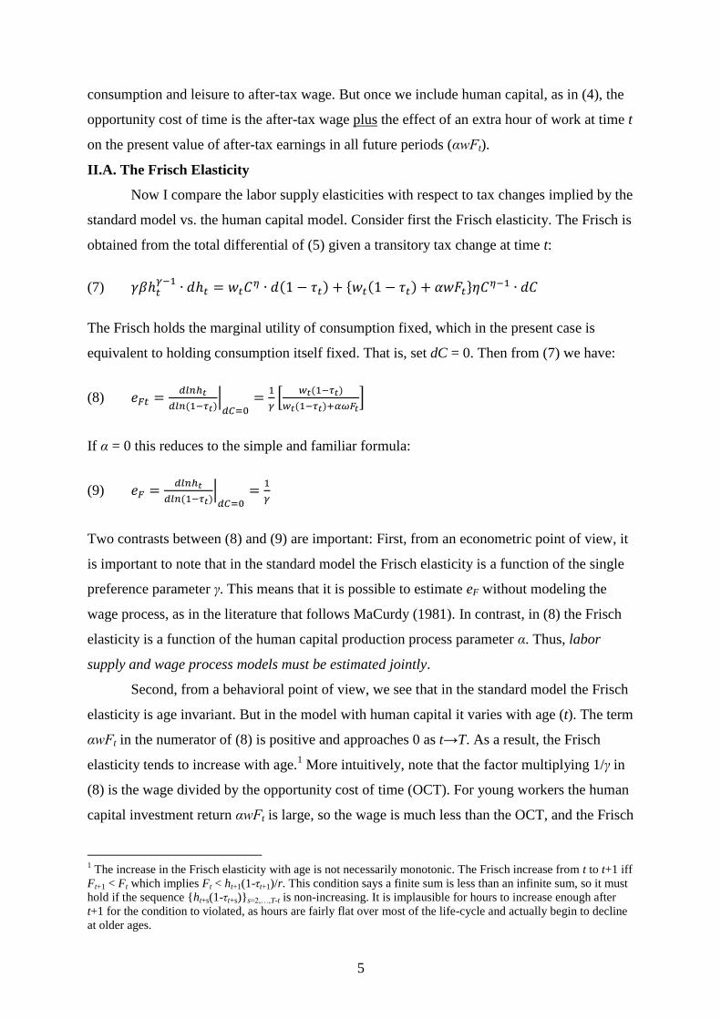
consumption and leisure to after-tax wage. But once we include human capital, as in (4), the

opportunity cost of time is the after-tax wage plus the effect of an extra hour of work at time t

on the present value of after-tax earnings in all future periods (αwFt).

II.A. The Frisch Elasticity

Now I compare the labor supply elasticities with respect to tax changes implied by the

standard model vs. the human capital model. Consider first the Frisch elasticity. The Frisch is

obtained from the total differential of (5) given a transitory tax change at time t:

(7) 𝛾𝛽ℎ𝑡𝛾−1

∙ 𝑑ℎ𝑡 = 𝑤𝑡𝐶𝜂 ∙ 𝑑(1 − 𝜏𝑡) + {𝑤𝑡(1 − 𝜏𝑡) + 𝛼𝑤𝐹𝑡}𝜂𝐶𝜂−1 ∙ 𝑑𝐶

The Frisch holds the marginal utility of consumption fixed, which in the present case is

equivalent to holding consumption itself fixed. That is, set dC = 0. Then from (7) we have:

(8) 𝑒𝐹𝑡 =𝑑𝑙𝑛ℎ𝑡

𝑑𝑙𝑛(1−𝜏𝑡)|

𝑑𝐶=0=

1

𝛾[

𝑤𝑡(1−𝜏𝑡)

𝑤𝑡(1−𝜏𝑡)+𝛼𝜔𝐹𝑡]

If α = 0 this reduces to the simple and familiar formula:

(9) 𝑒𝐹 =𝑑𝑙𝑛ℎ𝑡

𝑑𝑙𝑛(1−𝜏𝑡)|

𝑑𝐶=0=

1

𝛾

Two contrasts between (8) and (9) are important: First, from an econometric point of view, it

is important to note that in the standard model the Frisch elasticity is a function of the single

preference parameter γ. This means that it is possible to estimate eF without modeling the

wage process, as in the literature that follows MaCurdy (1981). In contrast, in (8) the Frisch

elasticity is a function of the human capital production process parameter α. Thus, labor

supply and wage process models must be estimated jointly.

Second, from a behavioral point of view, we see that in the standard model the Frisch

elasticity is age invariant. But in the model with human capital it varies with age (t). The term

αwFt in the numerator of (8) is positive and approaches 0 as t→T. As a result, the Frisch

elasticity tends to increase with age.1 More intuitively, note that the factor multiplying 1/γ in

(8) is the wage divided by the opportunity cost of time (OCT). For young workers the human

capital investment return αwFt is large, so the wage is much less than the OCT, and the Frisch

1 The increase in the Frisch elasticity with age is not necessarily monotonic. The Frisch increase from t to t+1 iff

Ft+1 < Ft which implies Ft < ht+1(1-τt+1)/r. This condition says a finite sum is less than an infinite sum, so it must

hold if the sequence {ht+s(1-τt+s)}s=2,…,T-t is non-increasing. It is implausible for hours to increase enough after

t+1 for the condition to violated, as hours are fairly flat over most of the life-cycle and actually begin to decline

at older ages.

6

elasticity is much less than1/γ. For workers close to retirement the human capital investment

return αwFt is small, and the wage is only slightly less than the OCT. Thus, the Frisch

elasticity for older workers is close to 1/γ.

The Frisch elasticity tells us the effect of a tax change holding lifetime wealth fixed.

But, more importantly, it tells us the approximate effect of transitory tax changes, as these

have small effects on lifetime wealth. Our results suggest that transitory tax changes will

have smaller labor supply effects than implied by the standard model (i.e., smaller than1/γ)

because they affect only a fraction of the opportunity cost of time. That is, a transitory tax

does not alter the returns to human capital investment.

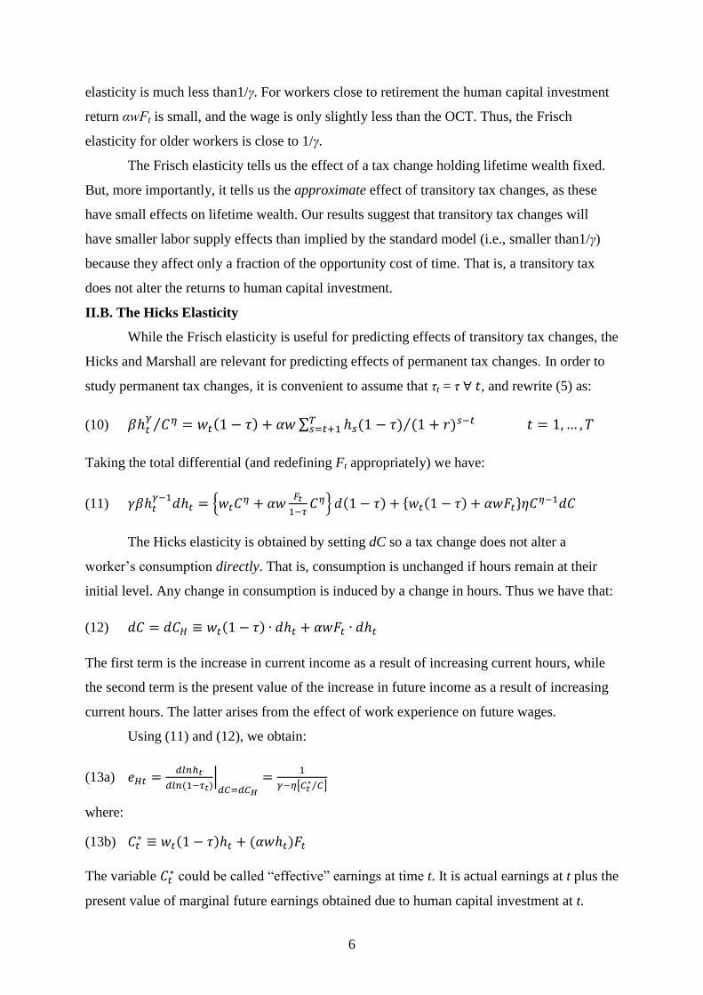
II.B. The Hicks Elasticity

While the Frisch elasticity is useful for predicting effects of transitory tax changes, the

Hicks and Marshall are relevant for predicting effects of permanent tax changes. In order to

study permanent tax changes, it is convenient to assume that τt = τ ∀ 𝑡, and rewrite (5) as:

(10) 𝛽ℎ𝑡𝛾

𝐶𝜂⁄ = 𝑤𝑡(1 − 𝜏) + 𝛼𝑤 ∑ ℎ𝑠(1 − 𝜏) (1 + 𝑟)𝑠−𝑡⁄𝑇𝑠=𝑡+1 𝑡 = 1, … , 𝑇

Taking the total differential (and redefining Ft appropriately) we have:

(11) 𝛾𝛽ℎ𝑡𝛾−1

𝑑ℎ𝑡 = {𝑤𝑡𝐶𝜂 + 𝛼𝑤𝐹𝑡

1−𝜏𝐶𝜂} 𝑑(1 − 𝜏) + {𝑤𝑡(1 − 𝜏) + 𝛼𝑤𝐹𝑡}𝜂𝐶𝜂−1𝑑𝐶

The Hicks elasticity is obtained by setting dC so a tax change does not alter a

worker’s consumption directly. That is, consumption is unchanged if hours remain at their

initial level. Any change in consumption is induced by a change in hours. Thus we have that:

(12) 𝑑𝐶 = 𝑑𝐶𝐻 ≡ 𝑤𝑡(1 − 𝜏) ∙ 𝑑ℎ𝑡 + 𝛼𝑤𝐹𝑡 ∙ 𝑑ℎ𝑡

The first term is the increase in current income as a result of increasing current hours, while

the second term is the present value of the increase in future income as a result of increasing

current hours. The latter arises from the effect of work experience on future wages.

Using (11) and (12), we obtain:

(13a) 𝑒𝐻𝑡 =𝑑𝑙𝑛ℎ𝑡

𝑑𝑙𝑛(1−𝜏𝑡)|

𝑑𝐶=𝑑𝐶𝐻

=1

𝛾−𝜂[𝐶𝑡∗ 𝐶⁄ ]

where: (13b) 𝐶𝑡

∗ ≡ 𝑤𝑡(1 − 𝜏)ℎ𝑡 + (𝛼𝑤ℎ𝑡)𝐹𝑡

The variable 𝐶𝑡

∗ could be called “effective” earnings at time t. It is actual earnings at t plus the

present value of marginal future earnings obtained due to human capital investment at t.

7

If α = 0 then equation (13) reduces to:

(14) 𝑒𝐻 =𝑑𝑙𝑛ℎ𝑡

𝑑𝑙𝑛(1−𝜏𝑡)|

𝑑𝐶=𝑑𝐶𝐻(𝛼=0)

=1

𝛾−𝜂

which is, as noted by MaCurdy (1983), the Hicks elasticity in the standard model.

Two contrasts between (13) and (14) are important. First, from an econometric point

of view, it is important to note that in the standard model the Hicks elasticity is a function of

two preference parameters, γ and η. Thus, it is possible to estimate eH without explicitly

modeling the wage process, given data on wages, hours and consumption, as in MaCurdy

(1983). In contrast, in equation (13) the Hicks elasticity is a function of the human capital

production process parameter α. Thus, to uncover the Hicks elasticity, one must jointly

estimate models of labor supply, consumption and the wage process.

Second, from a behavioral point of view, we see that in the standard model the Hicks

elasticity is age invariant. But in the human capital model it varies with age. How it varies

depends on the effective earnings variable 𝐶𝑡∗. The first component of 𝐶𝑡

∗, current earnings,

has a hump shape over the life-cycle, while second component, the human capital investment

return (αwhtFt), declines with age. Thus, it is ambiguous (and an empirical matter) how the

Hicks elasticity varies from youth to middle age. But both components of 𝐶𝑡∗ approach zero

as workers approach retirement. Thus, the Hicks elasticity for older workers is close to 1/γ. In

fact, both the Frisch and Hicks elasticities converge to (1/γ) as t→T. It is interesting that

while the human capital mechanism can only dampen the Frisch elasticity, it can either

dampen or amplify the Hicks, depending on the size of 𝐶𝑡∗ relative to C.

In the standard model it is well known that the Frisch elasticity must be greater than

or equal to the Hicks; that is, (1/γ) ≥ 1/(γ-η). There is equality only in the case of no income

effects (η=0). The reason the Frisch elasticity exceeds the Hicks is that Frisch compensation

is greater than Hicks compensation. But with the introduction of human capital the ranking

becomes ambiguous and age dependent.

Comparing (8) and (13), we see that the Hicks elasticity at age t exceeds the Frisch if:

(15) 1

𝛾−𝜂[𝐶𝑡∗ 𝐶⁄ ]

>1

𝛾[

𝑤𝑡(1−𝜏𝑡)

𝑤𝑡(1−𝜏𝑡)+𝛼𝑤𝐹𝑡] ⇒ 𝛼𝑤𝐹𝑡 >

(−𝜂)

𝛾

𝐶𝑡∗

𝐶𝑤𝑡(1 − 𝜏𝑡)

Strikingly, in the case of no income effects (η=0) this inequality must hold, so the Hicks

elasticity must exceed the Frisch. This is because permanent tax changes have a larger effect

on the price of time than transitory, and so a larger pure substitution effect. But income

8

effects work in the opposite direction. Thus, in general, (15) implies that the Hicks elasticity

will exceed the Frisch if the return to human capital investment (αwFt) is sufficiently large

relative to the strength of the income effect and the size of effective earnings (−𝜂𝐶𝑡∗). To see

why, note that as α↑ the Frisch falls, while as −𝜂𝐶𝑡∗↓ the Hicks increases.

Thus, once we introduce human capital, it is possible that permanent compensated tax

changes will have larger effects on current labor supply than transitory tax changes. This

result contradicts the conventional wisdom that transitory tax changes should have larger

effects than permanent changes. The fundamental reason for this outcome is that a permanent

tax change has a greater effect on the opportunity cost of time than a transitory tax change,

because it affects not only the current wage but also returns to human capital investment.

There are two important implications of this result: First, it may undermine the

argument for transitory tax cuts as an economic stimulus measure, while lending some

empirical support to the supply side argument for permanent compensated tax cuts. Second,

because the Frisch elasticity has been viewed as an upper bound on the Hicks, the large

literature based on MaCurdy (1981) that finds small estimates of the Frisch elasticity has

been interpreted as implying very small values of the Hicks as well, which in turn implies

small welfare effects of taxation. But if the Frisch > Hicks relation no longer holds, this

conclusion no longer follows.

II.C. The Marshallian Elasticity

Finally, we consider the Marshallian or uncompensated elasticity. The allows dC to

incorporate both incremental earnings due to changes in hours and the income effect due to

the change in the tax rate. In particular, we have:

(16) 𝑑𝐶 = 𝑑𝐶𝑀 ≡ 𝑤𝑡(1 − 𝜏) ∙ 𝑑ℎ𝑡 + 𝛼𝑤𝐹𝑡 ∙ 𝑑ℎ𝑡 +𝐸𝑡

1−𝜏∙ 𝑑(1 − 𝜏)

where Et denotes the present value of after-tax earnings:

(17) 𝐸𝑡 ≡ ∑𝑤𝑠(1−𝜏)ℎ𝑠

(1+𝑟)𝑠−𝑡𝑇𝑠=𝑡

Using (11) and (16), we obtain:

(18) 𝑒𝑀𝑡 =𝑑𝑙𝑛ℎ𝑡

𝑑𝑙𝑛(1−𝜏𝑡)|

𝑑𝐶=𝑑𝐶𝑀

=1+𝜂[𝐸𝑡 𝐶⁄ ]

𝛾−𝜂[𝐶𝑡∗ 𝐶⁄ ]

Notice that the denominator of the Marshallian elasticity is identical to the Hicks. The

income effect comes in through the additional 𝜂[𝐸𝑡 𝐶⁄ ] term in the numerator. If α = 0 then

9

equation (18) reduces to:

(19) 𝑒𝑀 =𝑑𝑙𝑛ℎ𝑡

𝑑𝑙𝑛(1−𝜏𝑡)|

𝑑𝐶=𝑑𝐶𝑀(𝛼=0)

=1+𝜂

𝛾−𝜂

which is the Marshallian elasticity in the standard model.

Comparing (18) and (19) we again see that the introduction of human capital again

has two effects: (i) it makes the Marshallian elasticity a function of both preference and wage

process parameters, and (ii) it makes the elasticity a function of age.

Of course, the income effect term 𝜂[𝐸𝑡 𝐶⁄ ] in (18) is non-positive, so the Marshallian

elasticity must be less than (or equal to) the Hicks. The Marshallian elasticity is positive only

if 1 + 𝜂(𝐸𝑡 𝐶⁄ ) ≥ 0. Thus, even the sign of the Marshallian elasticity may vary with age.

Strikingly, it is ambiguous whether the Marshallian elasticity is greater or less than

the Frisch. Comparing (8) and (18), we see that the Marshall is greater than the Frisch if:

(20) 𝛼𝑤𝐹𝑡 > [(−𝜂)

𝛾

𝐶𝑡∗

𝐶− 𝜂

𝐸𝑡

𝐶] 𝑤𝑡(1 − 𝜏𝑡)

1

1+𝜂(𝐸𝑡 𝐶⁄ ) 𝑎𝑛𝑑 1 + 𝜂(𝐸𝑡 𝐶⁄ ) > 0

If there are no income effects (η=0), this condition reduces to αwFt > 0, so the Marshall must

exceed the Frisch if there are any human capital effects. Again, this is because a permanent

tax change has a larger effect on the opportunity cost of time than a transitory one.

Once we allow for income effects, we see that the threshold in (20) is greater than that

in (15). The human capital effect αwFt must be stronger in order for the Marshall to exceed

the Frisch. Finally, as we discussed in Section II.B, the term 𝐶𝑡∗ 𝐶⁄ may be greater than or less

than one, and the same is true of 𝐸𝑡 𝐶⁄ . But it is clear that both 𝐶𝑡∗and Et approach zero as

workers approach retirement. As a result, the Marshall, Hicks and Frisch all converge to the

same value (1/γ) as workers get older.

II.D. Quantifying the Bias From Ignoring Human Capital

As I noted in the introduction, if human capital is important but we ignore it in

estimation, it will cause bias in estimates of preference parameters and labor supply

elasticities. But how severe is this problem likely to be? Is it quantitatively important? To

address this question, it is useful to work with a simple two-period version of our model.

If T=2 then the first order conditions for hours are:

(21) 𝛽1ℎ1𝛾

𝐶𝜂⁄ = 𝑤1(1 − 𝜏1) + 𝜌𝛼𝑤ℎ2(1 − 𝜏2) 𝛽2ℎ2𝛾

𝐶𝜂⁄ = 𝑤2(1 − 𝜏2)

Note that at t=1 the opportunity cost of time is augmented by the term ραw1h2(1-τ2), which

captures the effect of an hour of work at t=1 on the present value of earnings at t=2.

10

Using (21) we can obtain the following hours change equation:

(22) 𝑙𝑛(ℎ2 ℎ1⁄ ) =1

𝛾𝑙𝑛 [

𝑤2(1−𝜏2)

𝑤1(1−𝜏1)+𝜌𝛼𝑤ℎ2(1−𝜏2)] + 휀

where ε ≡ (1/γ)ln(β1/β2) is a shock to tastes for work (as in MaCurdy (1981)).

Equation (22) makes clear why the conventional method of regressing hours growth

on wage growth understates labor supply elasticities and overstates γ. The effective wage rate

at t=1 is understated by the failure to account for the human capital term ραw1h2(1-τ2) in the

denominator of (22). Thus, effective wage growth from t=1 to t=2 is exaggerated. As a result,

the responsiveness of hours of work to changes in the price of time is understated.

We can get a better sense of the magnitude of the problem by considering the

regression of hours changes on wage changes:

(23) 𝑙𝑛(ℎ2 ℎ1⁄ ) = Γ𝑙𝑛 [𝑤2(1−𝜏2)

𝑤1(1−𝜏1)] + 𝜐

By running the population regression we obtain:

(24) Γ =1

𝛾𝑙𝑛 [

𝑤2(1−𝜏2)

𝑤1(1−𝜏1)+𝜌𝛼𝑤ℎ2(1−𝜏2)] 𝑙𝑛 [

𝑤2(1−𝜏2)

𝑤1(1−𝜏1)]⁄

Thus, the estimate of (1/γ) is biased downward by a factor equal to the ratio of the rate of

growth in the effective wage rate to the rate of growth in the observed wage rate. As the

Frisch, Hicks and Marshall elasticities all have the preference parameter γ in their

denominators, inferences about all three elasticities will be biased downwards.

To assess how large the bias is likely to be, we need a plausible value for the 𝜌𝛼𝑤ℎ2

term in (24). Given a two period model where each period corresponds to 20 years, it is

plausible in light of existing estimates that αwh1, the percent growth in the wage over 20

years, is on the order of 33% to 50%.2 So take the conservative value of αwh1 = 33%. A

reasonable figure for hours growth over the first 20 years of the working life is roughly 20%

(see, e.g., Imai and Keane (2004) or the descriptive regressions in Pencavel (1986)). So

assume that h2 is 20% greater than h1. Then αwh2 is roughly 40%. Let ρ = 1/(1.03)20

= 0.554.

Then we obtain ραwh2 = 22%. Finally, assume that τ1 = τ2, and normalize w1(1- τ1). In this

example, wage growth is 33%, but the growth in the opportunity cost of time is only

1.33/1.22 = 9%.

2 For instance, using the PSID, Geweke and Keane (2000) estimate that for men with a high school degree,

average earnings growth from age 25 to 45 is 33% (most of which is due to wage growth). For men with a

college degree the estimate is 52%. They also find that earnings growth essentially ceases after about age 45.

11

Given these parameter values, the bias term in (24) is ln(1.33/1.22)/ln(1.33) = 0.30.

Thus, according to (24) our estimates of (1/γ) will be biased down by a factor of roughly 3.3.

So, for reasonable parameter values, we see that the bias from ignoring capital is substantial.

An important point is that instruments cannot be used to solve the problem of

endogenous wage formation. To see this rewrite (22) as:

(25) 𝑙𝑛(ℎ2 ℎ1⁄ ) =1

𝛾𝑙𝑛 [

𝑤2(1−𝜏2)

𝑤1(1−𝜏1)] + {휀 +

1

𝛾𝑙𝑛 [

𝑤1(1−𝜏2)

𝑤1(1−𝜏1)+𝜌𝛼𝑤ℎ2(1−𝜏2)]}

The composite error term (in curly brackets) includes the ratio of the first period wage to the

opportunity cost of time. Any variable that affects the growth rate of after-tax wages will be

correlated with this ratio as well.

III. Simulations of a Two-Period Model

In this section, I use a simple two-period version of the model of Section II to

illustrate some ways in which the introduction of human capital affects the behavior of the

life-cycle model. The only change is that the human capital production function is made more

realistic, as closed form solutions are no longer needed.

III.A. Two-Period Model Calibration

To calibrate the two-period model, we may think of each period as 20 years out of a

40-year working life (e.g., 25 to 44 and 45 to 64). I assume a real annual interest rate of 3%.

As 1/(1+.03)20

= 0.554, this implies a 20 year interest rate of r = .806. Thus, I assume the

discount factor is ρ = 1/(1+r) = 0.554. I set the tax rates to τ1 = τ2 = .40 in the baseline model.

Turning to the wage function, in contrast to the simple function assumed for analytical

convenience in Section II, equation (4), here I assume the more realistic:

(26) 𝑤2 = 𝑤1𝑒𝑥𝑝 (𝛼ℎ1 − 𝜅ℎ1

2

100− 𝛿) ⇒ 𝑙𝑛𝑤2 = 𝑙𝑛𝑤1 + 𝛼ℎ1 − 𝜅

ℎ12

100− 𝛿

This is similar to a Mincer log earnings function, where w1 is the initial skill endowment, and

there is a quadratic in hours (experience). But I also include a depreciation term δ, which

causes earnings to fall if the person does not work sufficient hours in period one. Keane and

Wolpin (1997) find depreciation is important.

I consider three values of the utility function parameter η that governs the strength of

the income effect, η ∈ {-.50, -.75 and -1.0}. Two (of the very few) studies that estimate life-

cycle models with both savings and human capital, and that also assume CRRA utility, are

Keane and Wolpin (2001) and Imai and Keane (2004). They estimate η ≈ -.5 and η ≈ -.75,

12

respectively.3 I also consider the η = -1.0 case because it is widely used in macro models (i.e.,

U=log(C) so income and substitution effects cancel and there is balanced growth).

Of course, the value of γ is the subject of controversy. Most prior micro estimates of

(1/γ) using the MaCurdy (1981) approach are quite small – i.e., around .30 or less (see Keane

(2011)). At the same time, many macro economists have argued that values of 2 or greater are

needed to explain business cycle fluctuations using standard models (see Prescott (1986,

2006)). Imai and Keane (2004) is a major exception to the prior micro data literature, as they

estimate that (1/γ) = 3.7. They argue, for reasons similar to those discussed in Section II.D,

that failure to account for human capital led prior work to severely understate (1/γ).4

Given the controversy over γ, I examine the behavior of the model for a wide range of

values. Specifically, I look at γ ∈ {0, 0.25, 0.50, 1, 2, 4}. But I often focus on γ = 0.50, which

I consider plausible in light of Imai and Keane (2004) and Keane and Rogerson (2010).

Finally, β is a scaling parameter that depends on the units for hours and consumption,

and has no bearing on the substantive behavior of the model. Thus, in each simulation, I set β

so optimal hours are 100 in the model without human capital (α=0). The initial wage w1 is

also set to 100. These values were chosen purely for ease of interpreting the results.

Given this normalization, we can think of h=100 as corresponding (roughly) to full-

time work and h=50 to part-time work. I calibrate the model so that: (i) a person must work at

least part-time at t=1 for the wage not to fall at t=2, and (ii) the return to additional work falls

to zero at h=200. Given these constraints, the wage function reduces to:

(27) 𝑤2 = 𝑤1𝑒𝑥𝑝 (𝛼ℎ1 −𝛼

4

ℎ12

100−

175

4𝛼)

Thus, the single parameter α determines how work experience maps into human capital.

In order to obtain the wage growth of roughly 33% to 50% that is observed for men

from age 25 to age 45, it is necessary to set α in the .008 to .010 range. So I consider these

plausible values. However, I will also consider a range of other α values, to learn how the

behavior of the model changes when human capital is more or less important.

The calibrated model generates reasonable values for hours growth. For instance, the

model with α = .008, η = -.50, and γ = .50 gives a 10% increase in hours from t=1 to t=2. As a

3 Shaw (1989) was the first to estimate a dynamic model with both human capital and saving. But she used

translog utility, so the estimates are not useful for calibrating (1). Goeree, Holt and Palfrey (2003) present

experimental evidence, as well as evidence from field auction data, in favor of η ≈ -.4 to -.5. Bajari and Hortacsu

(2005) estimate η ≈ -.75 from auction data. 4 Some other exceptions are Heckman and MaCurdy (1982), who obtain 2.3 for married women in the PSID,

and French (2005), who obtains 1.33 for 60 year olds in the PSID. Recall from our results in Section II.A that

downward bias in estimates of (1/γ) should be less for older workers.

13

point of comparison, for the 1956-65 birth cohort, McGrattan and Rogerson (1998) report

average hours growth of 12% from ages 25-34 to ages 35-44.5 Of course, a simple two-period

must abstract from the subsequent decline in hours as older workers approach retirement.

III.B. Simulations of Two-Period Model – Standard Model without Human Capital

Next I use the two-period model to simulate labor supply elasticities. This helps to

clarify how introduction of human capital affects the behavior of the life-cycle model.

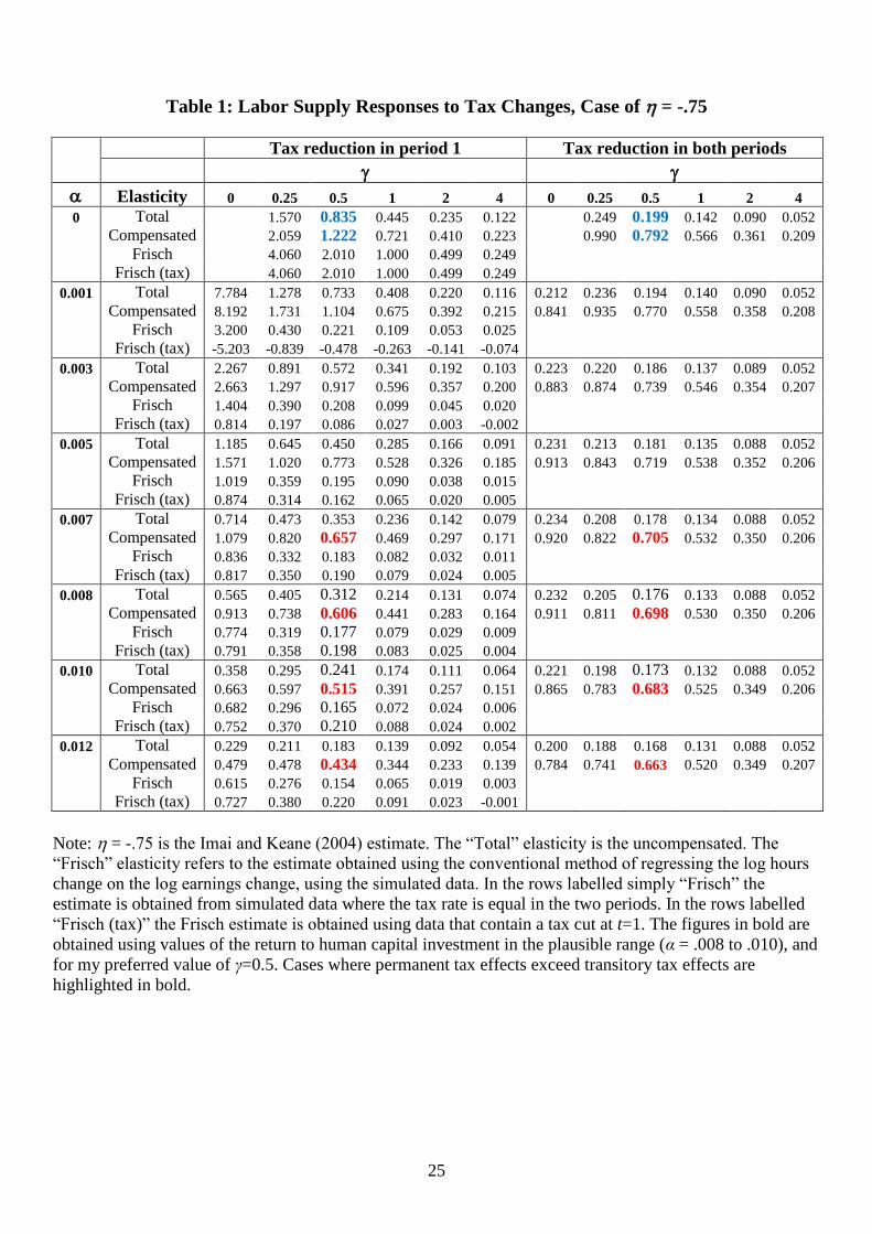
Table 1 presents results for models calibrated with the Imai-Keane (2004) estimate of

η = -.75. The left panel shows elasticities with respect to temporary tax changes at t=1. The

first two rows show uncompensated (total) and compensated (Hicks) elasticities. The next

two rows show the Frisch elasticity calculated in the conventional way – the growth rate of

hours divided by the growth rate of wages. The right panel of Table 1 shows elasticities with

respect to permanent tax changes (i.e., changes that apply in both periods).

As a point of comparison, the first four rows of Table 1 show results for the standard

model with no human capital accumulation (α = 0). Then the lower rows show results for

progressively higher values of α. The columns correspond to different values of γ.

Consider first the standard model (α = 0) with γ = .50, which is a common value in

calibrating real business cycle models. Then, the Marshallian elasticity is (1+η)/(γ-η) = 0.20,

the Hicks (compensated) elasticity is 1/(γ-η) = 0.80, and the Frisch elasticity is 1/γ = 2.0. As

we see in the first three rows of Table 2, the simulated values of these elasticities correspond

closely to the theoretical values. Slight differences arise because we are taking finite

difference derivatives (i.e., we increase (1-τ) by 1%).

Notice that, in the present context, elasticities with respect to transitory tax changes at

t=1 are smaller than the Frisch elasticity. This is because, with only two periods, a change in

the t=1 tax rate leads to a non-trivial change in consumption (even with Hicks compensation).

Keane (2009) shows that, in the standard model, in the two-period case, the uncompensated

and compensated labor supply elasticities with respect to temporary tax changes at t=1 are:

(28) 𝜕𝑙𝑛ℎ1

𝜕ln (1−𝜏1)= [

1+𝜂

𝛾−𝜂] − [

𝜂

𝛾−𝜂

1+𝛾

𝛾

1

2+𝑟]

𝜕𝑙𝑛ℎ1

𝜕ln (1−𝜏1)|

𝑐𝑜𝑚𝑝=

1

𝛾

1

2+𝑟+

1

𝛾−𝜂

1+𝑟

2+𝑟

These equations give values of 0.84 and 1.228, which align closely with the values of 0.835

and 1.222 obtained in the simulation. As expected, these elasticities with respect to transitory

tax cuts greatly exceed those with respect to permanent tax cuts.

5 Exceptions are the models with γ=0, which generate unrealistically large hours growth, and models with γ=4,

which generate unrealistically small hours growth. See Keane (2009) for more details on the calibration.

14

III.C. Simulations of Two-Period Model – A Small Human Capital Effect

Rather surprisingly, the introduction of just a small human capital effect leads to some

important changes in results. The second panel of Table 1 presents results when the human

capital effect is set at the very low level of α = .001. Strikingly, even this small value renders

the conventional method of estimating the Frisch elasticity – i.e., taking the ratio of hours

growth to wage growth – completely unreliable.6

For instance, with γ = 0.50 and tax rates fixed, hours increase by 0.72% from t=1 to

t=2 while the wage increases by 3.25%. Taking the ratio, the conventional method would

infer a Frisch elasticity of only 0.221. In contrast, the true value of (1/γ) is 2.0 and the

compensated elasticity with respect to a transitory tax cut in period one is 1.104.

One might surmise that the conventional method of estimating the Frisch is severely

biased because the wage change from t=1 to t=2 in the baseline model (with a fixed tax rate)

is entirely endogenous – i.e., it results entirely from human capital investment. One might

further surmise that if the data contained a source of exogenous variation, such as an

exogenous tax change, one could infer γ more reliably.

Surprisingly, this intuition is fundamentally flawed. The row labelled “Frisch (tax)” in

Table 2 reports Frisch elasticities calculated in the conventional manner in a regime with a

temporary 1% tax cut in t=1. In the γ = 0.50 case we see the estimate is -.478, which is not

even the correct sign! Why? The tax cut causes labor supply to increase in period 1, which, in

turn, increases the wage in period 2. But despite the wage increase, hours actually decline in

period 2. This is because (i) the tax cut is removed, and (ii) the human capital investment part

of the opportunity cost of time is removed. Thus, despite the fact that the wage is higher at

t=2, the opportunity cost of time is lower, leading to lower hours.

This discussion clarifies the point that a strictly exogenous shift in the wage path

cannot exist in a model with human capital. For instance, a higher after-tax wage at t=1

increases hours at t=1, but it also raises the wage at t=2 via the human capital effect. So a t=1

tax cut does not cause an exogenous change in the wage profile, because the wage at t=2 is

altered by the behavioral response.

This has fundamental implications for estimation of wage elasticities. As I noted in

Section II.D, if experience alters wages, methods that rely on exogenous wage variation

(instruments) will not work. One must model the joint wage/labor supply process.

6 Of course, econometric studies that estimate the Frisch elasticity by regressing hours changes on wage changes

use more complex IV techniques, designed to deal with measurement error in wages, heterogeneity in tastes for

work, and unanticipated wage changes. We do not have any of those problems here, so the appropriate estimator

boils down to just taking the ratio of the percentage hours change to the percentage wage change.

15

III.D. Simulations of Two-Period Model – Plausible Human Capital Effects

In this section I consider the behavior of the model with plausible returns to work

experience. As I noted in Section II.A, this requires α in the range of .008 to .010, gives wage

growth of roughly 33% to 50%, and hours growth of 10% to 15%.

The left panel of Table 1 reports labor supply elasticities with respect to transitory

(t=1) tax cuts. The first thing to note is that both uncompensated and compensated elasticities

drop substantially when human capital is included in the model. For example, the elasticity

falls from 1.222 in the no human capital case to .606 in the α=.008 case. This is consistent

with our finding in Section II.A that human capital reduces responses to temporary tax cuts.

Recall from Sections II.B-II.C that effects of human capital on Hicks and Marshall

elasticities are ambiguous. In the right panel of Table 1, we see that compensated and

uncompensated elasticities with respect to permanent tax changes tend to decline as α

increases. But the decline is modest (and there are a few exceptions).

As human capital dampens transitory tax effects more than permanent, it creates the

possibility that permanent tax changes can have larger effects than transitory. For instance,

when α=.008 and γ = 0.50, the compensated elasticity of labor supply at t=1 with respect to a

temporary tax cut is 0.606, but that with respect to a permanent tax cut is greater, 0.698. So, it

is indeed possible for permanent tax changes to have larger effects than transitory at plausible

parameter values, at least for compensated tax changes.7 In the next section, we’ll see this can

be true in the uncompensated case as well.

Finally, in Table 1 we also see that the conventional method of estimating the Frisch

elasticity gives results 3 to 4 times smaller than compensated elasticities for both permanent

and temporary tax changes. This illustrates how the low estimates of the Frisch elasticity in

the literature cannot be viewed as an upper bound on compensated elasticities.8

III.D. Simulations of Two-Period Model – Sensitivity to Income Effects

III.D.1. The Case of η = -.50

In this section I consider the behavior of the model with η = -.5, which is the value

estimated by Keane and Wolpin (2001). This implies weaker income effects than in the

previous simulations. The results are presented in Table 2. Focus again on the γ = 0.50 case.

In the model without human capital (α=0), the uncompensated elasticity with respect to a

7 The uncompensated elasticity of labor supply at t=1 with respect to a temporary tax cut at t=1 is 0.312, while

that with respect to a permanent tax cut is 0.176. So the income effect is strong enough that that temporary tax

changes have larger effects than permanent in the uncompensated case. 8 In fact, the Frisch elasticities do not even give upper bounds for uncompensated elasticities. E.g., in the

α=.008, γ = 0.50 case the two methods of calculating the Frisch elasticity produce values of 0.177 and 0.198,

while the uncompensated elasticity for a t=1 tax cut is 0.312.

16

temporary tax cut at t=1 is, as expected, almost exactly twice as large as that with respect to a

permanent tax cut (1.03 vs. 0.50). But with plausible returns to work experience (α = .008),

the uncompensated elasticity with respect to a permanent tax cut is greater than that with

respect to a temporary tax cut (0.445 vs. 0.420).

These results are consistent with the theoretical analysis in Sections II.B and II.C.

There we found that permanent tax changes can have larger effects than transitory if and only

if the return to human capital investment is greater than a bound that is increasing in the

strength of the income effect. And for uncompensated tax changes the bound is greater. In

Table 1 we found cases where compensated elasticities with respect to permanent tax changes

exceeded those with respect to transitory. Now, with weaker (but still plausible) income

effects, we obtain this outcome for uncompensated tax changes.

Otherwise, the results in Table 2 are broadly similar to those in Table 1. Elasticities

with respect to permanent tax changes decline modestly as the strength of the human capital

affect increases. In contrast, elasticities with respect to transitory tax changes decline sharply.

The conventional method of estimating the Frisch elasticity produces sharply downward

biased estimates. These are much smaller than the true elasticities with respect to transitory

tax changes, whether compensated or uncompensated.

III.D.2. The Case of Log Utility (Income and Substitution Effects Cancel)

The previous sections presented results for values of η such that substitution effects

dominate income effects (η>-1). But macro models often assume log(C) utility to generate

balanced growth paths. Thus, it is also interesting to consider the case of η= -1. To conserve

space I only give an overview of the results.

Of course, the uncompensated elasticity with respect to permanent tax cuts is always

zero, as income and substitution effects cancel. The uncompensated elasticities of t=1 labor

supply with respect to transitory tax cuts are 0.24, 0.18 and 0.13 in the α=0.008, 0.010 and

0.012 cases, respectively. So, exactly as expected, with log utility transitory tax cuts must

have larger effects than permanent tax cuts in the uncompensated case.

But in the compensated case this outcome is reversed. Compensated elasticities of t=1

labor supply with respect to transitory tax cuts are 0.56, 0.48 and 0.42 for the α=0.008, 0.010

and 0.012 cases, respectively. But for permanent tax cuts the figures are 0.57, 0.56 and 0.55.

A similar pattern holds for all γ in the 0.25 to 4 range.9 Thus, for plausible human capital

effects, and for all plausible γ, permanent tax effects are larger than transitory tax effects.

9 For example, if γ=2.0, which conforms closely with conventional wisdom, the compensated elasticity of t=1

labor supply with respect to transitory tax cuts is 0.27, 0.24 and 0.22 for the α=0.008, 0.010 and 0.012 cases,

17

IV. Simulations of the Imai-Keane Model (Short vs. Long Run Tax Effects)

A number of the theoretical predictions in Section II concern how labor supply

elasticities vary with age. This can only be examined using a multi-period model. It is also

important to compare the long-run vs. short run effects of tax changes, and how these are

affected by human capital. This requires a multi-period model as well.

In this section I use the Imai and Keane (2004) model to simulate effects of various

types of tax changes. To my knowledge, this is the only micro model that attempts to fit asset,

hours and wage data over the whole working life.10

Because it generates life-cycle paths from

age 20 to 65, it can be used to simulate both age specific labor supply elasticities and the

long-run effects of permanent tax changes. The basic setup of the model is as follows:

The Imai-Keane model assumes the same utility function as MaCurdy (1981). There

are annual decision periods from age 20 to 65. At age 65 agents must retire, and there is a

terminal value function that depends on assets (to generate a motive for retirement savings).

The model contains a complex human capital production function that generalizes the simple

2-period model in several ways. In particular, it accommodates complimentarity between the

stock of human capital and hours of work in the production of skill. Such complimentarity is

quite evident in the data. Production function parameters are also allowed to vary in a flexible

way with education and age. Wages are stochastic, and wage shocks exhibit persistence over

time. Agents can borrow/lend across periods, and there are age varying tastes.

The model is fit to white males from the NLSY79 born in 1958-65 and followed from

age 20 to 36. Imai and Keane (2004) document that the model produces a good in-sample fit

to assets, hours and wages, both in terms of typical age profiles and dynamics/transition rates

(e.g., it captures observed persistence in individual wages quite accurately). It also generates

reasonable out-of-sample forecasts past age 36. For instance, the model predicts an hours

decline from ages 45-54 to 55-64 of 53%.11

This is close to the 47% figure for this cohort

projected by McGrattan and Rogerson (1998). Also, when simulated data from the Imai-

Keane model is used to estimate conventional labor supply functions, it gives conventional

(i.e., small) elasticities. As the model provides a good fit to wage, hours and asset patterns –

both in and out-of-sample – it seems credible to use it to predict labor supply responses.

respectively. But for permanent tax cuts these figures are 0.32, 0.31 and 0.31. Thus, the permanent tax effects

are 20% to 40% greater than transitory effects. 10

Two other papers that fit assets, hours and wages are Van der Klauuw and Wolpin (2008) and Keane and

Wolpin (2001). The former simulates behavior of older workers, while the later focuses on youth. 11

A limitation of the Imai-Keane model is it assumes interior solutions for hours, so it cannot generate complete

retirement prior to age 65. But this limitation should not be exaggerated. In the 2008 CPS, 70% of men aged 55-

64 still worked, and 52% of men aged 62-64 still worked (see Purcell (2009)).

18

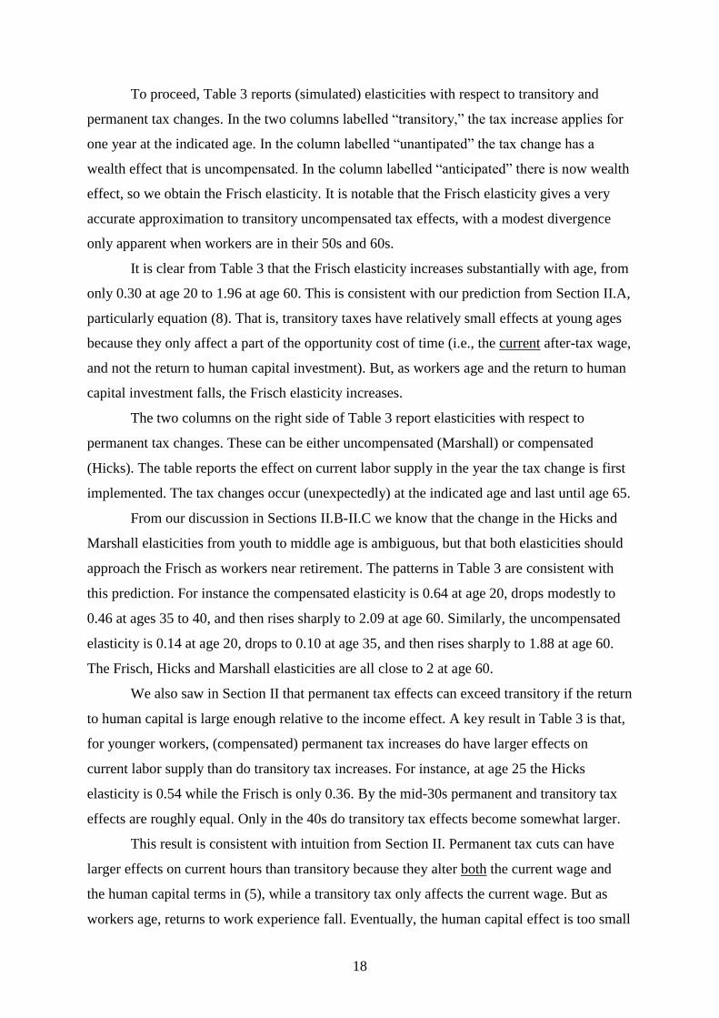
To proceed, Table 3 reports (simulated) elasticities with respect to transitory and

permanent tax changes. In the two columns labelled “transitory,” the tax increase applies for

one year at the indicated age. In the column labelled “unantipated” the tax change has a

wealth effect that is uncompensated. In the column labelled “anticipated” there is now wealth

effect, so we obtain the Frisch elasticity. It is notable that the Frisch elasticity gives a very

accurate approximation to transitory uncompensated tax effects, with a modest divergence

only apparent when workers are in their 50s and 60s.

It is clear from Table 3 that the Frisch elasticity increases substantially with age, from

only 0.30 at age 20 to 1.96 at age 60. This is consistent with our prediction from Section II.A,

particularly equation (8). That is, transitory taxes have relatively small effects at young ages

because they only affect a part of the opportunity cost of time (i.e., the current after-tax wage,

and not the return to human capital investment). But, as workers age and the return to human

capital investment falls, the Frisch elasticity increases.

The two columns on the right side of Table 3 report elasticities with respect to

permanent tax changes. These can be either uncompensated (Marshall) or compensated

(Hicks). The table reports the effect on current labor supply in the year the tax change is first

implemented. The tax changes occur (unexpectedly) at the indicated age and last until age 65.

From our discussion in Sections II.B-II.C we know that the change in the Hicks and

Marshall elasticities from youth to middle age is ambiguous, but that both elasticities should

approach the Frisch as workers near retirement. The patterns in Table 3 are consistent with

this prediction. For instance the compensated elasticity is 0.64 at age 20, drops modestly to

0.46 at ages 35 to 40, and then rises sharply to 2.09 at age 60. Similarly, the uncompensated

elasticity is 0.14 at age 20, drops to 0.10 at age 35, and then rises sharply to 1.88 at age 60.

The Frisch, Hicks and Marshall elasticities are all close to 2 at age 60.

We also saw in Section II that permanent tax effects can exceed transitory if the return

to human capital is large enough relative to the income effect. A key result in Table 3 is that,

for younger workers, (compensated) permanent tax increases do have larger effects on

current labor supply than do transitory tax increases. For instance, at age 25 the Hicks

elasticity is 0.54 while the Frisch is only 0.36. By the mid-30s permanent and transitory tax

effects are roughly equal. Only in the 40s do transitory tax effects become somewhat larger.

This result is consistent with intuition from Section II. Permanent tax cuts can have

larger effects on current hours than transitory because they alter both the current wage and

the human capital terms in (5), while a transitory tax only affects the current wage. But as

workers age, returns to work experience fall. Eventually, the human capital effect is too small

19

for the bound in (15) to be satisfied, and transitory taxes begin to have a larger current effect

than permanent taxes.

As we saw in Section II.C it is theoretically possible for uncompensated permanent

tax effects to exceed transitory tax effects. But, as we see in Table 3, the income effect is too

strong (relative to the human capital effect) for this to occur in practice.

So far, I have only discussed effects of tax changes on current period hours, or what

could be called short-run tax effects. Table 4 examines the long-run impact of permanent tax

changes. That is, I simulate the impact of a permanent change in the tax rate on earnings that

starts at age 20 and lasts through age 65.

First, consider the elasticity of lifetime hours, from age 20 to 65. As we see in Table

4, the uncompensated and compensated elasticities with respect to permanent tax changes are

0.4 and 1.3, respectively. Notably, the compensated elasticity implied by the Imai and Keane

parameter estimates in the standard model without human capital (a la MaCurdy (1981)) is

1/(γ-η) = 1/(.262+.736) ≈ 1.0. Thus, the human capital mechanism amplifies the compensated

elasticity of lifetime hours by 30% (from 1.0 to 1.3).

Second, Table 4 also reports elasticities of hours at selected ages. As we see, a

permanent tax increase reduces hours much more at older ages than at young ages. The effect

of a permanent tax change grows with age for two reasons: First, as I discussed in Section II,

as workers get older the after-tax wage makes up a larger fraction of the opportunity cost of

time. Second, a permanent tax hike slows the rate of human capital accumulation, which

produces a “snowball” effect on wages:

If a worker reduces his hours at time t, he will have a lower wage at time t+1. This

causes him to work even less at time t+1, leading to a lower wage at t+2, etc.. If we use the

model to simulate a 5% permanent tax increase starting at age 25, then by age 40 a worker’s

wage is reduced by only 1.0%, but by age 55 his wage is reduced by 3.6%, and by age 65 the

reduction is 11.6%. This lowering of pre-tax wages creates an additional work disincentive,

beyond the direct effect of the tax. And this disincentive becomes quite large at older ages.

Thus, we see that the human capital mechanism amplifies the effect of permanent tax

changes in the long run. This result has important implications for the growing literature that

attempts to estimate labor supply elasticities by looking at responses to major tax reforms

(see Saez et al (2011) or Keane (2011) for reviews). This literature adopts a difference-in-

difference approach and generally focuses on short-run responses. The results presented here

suggest that a short-run focus may cause one to seriously understate responses to taxes.

20

VII. Conclusion

When human capital is added to the standard life-cycle labor supply model, the wage

no longer equals the opportunity cost of time. Rather, the opportunity cost of time is the wage

plus the return to work experience. This has important implications for how workers respond

to taxes, and for proper estimation of labor supply elasticities.

There are three key econometric implications of adding human capital to the life-cycle

model. First, labor supply elasticities are no longer functions of preference parameters alone.

Instead, they also depend on parameters of the wage process. As a result, the conventional

GMM procedure for estimating elasticities and preferences without the need to specify the

wage process is no longer valid. One must specify and estimate the wage process as well.

Second, the conventional GMM procedure that ignores human capital will lead to

severely upward biased estimates of the degree of curvature of utility in hours (denoted by γ

in our model). This in turn, leads to downward biased estimates of labor supply elasticities. In

fact, given human capital, the data appear consistent with much larger labor supply

elasticities than conventional wisdom suggests.

Third, in the presence of human capital, effects of permanent tax changes on labor

supply grow over time, as a tax change affects not only the current after-tax wage but also the

rate of human capital investment. This has important implications for the growing literature

that attempts to estimate labor supply elasticities by looking at responses to major tax reforms

(see Saez et al (2011) or Keane (2011) for reviews). The short-run focus of most of this

literature may lead it to understate responses to taxes.

The introduction of human capital also has a number of important behavioral

implications. First, labor supply elasticities become a function age. The Frisch elasticity is

reduced for young workers, but it grows with age, approaching (1/γ) in our model as workers

near retirement. The age paths of the Hicks and Marshall elasticities are ambiguous, but they

also rise to a level close to the Frisch elasticity as workers near retirement. So a strong

prediction of the human capital model is that labor supply elasticities should be much greater

for older workers than for younger workers.

Second, contrary to conventional wisdom, it is possible for permanent tax changes to

have larger effects on current labor supply than transitory changes. This is because a

permanent tax alters both the current wage and the future return to human capital investment.

Thus, a permanent tax has a larger effect on the opportunity cost of time. Of course,

permanent tax changes also have larger income effects. So the condition for permanent taxes

to have larger effects than transitory is that returns to human capital investment must be

21

sufficiently large relative to income effects. In simulations of the labor supply model of Imai

and Keane (2004), I find that permanent tax changes are likely to have larger effects than

transitory for workers under 35 (for whom returns to work experience are large).

Third, human capital amplifies the response to permanent tax changes in the long-run.

This is because a permanent tax increase slows the rate of human capital accumulation, which

amplifies the effect on after-tax wages in the long-run. This in turn causes labor supply to fall

disproportionately at older ages. For example, simulation of the Imai-Keane model generates

a compensated elasticity of only 0.54 at age 25, but this rises to 3.9 at age 60.

Another way to view this phenomenon is to note that the preference parameters in the

Imai-Keane model (γ and η) imply a compensated (Hicks) elasticity of about 1.0 in a world

with no human capital. But simulation of their model generates a compensated elasticity of

lifetime hours of 1.30. Thus, the impact on lifetime hours is 30% greater than if the human

capital mechanism were shut down.

It should be noted that human capital reduces the Hicks elasticity at young ages (e.g.,

from 1.0 to 0.54 at age 25) while increasing it at older ages (e.g., from 1.0 to 3.9 at age 60).

Thus a permanent tax increase pivots the entire hours profile, shifting relatively more labor

supply to younger ages. However, our results indicate that, overall, human capital amplifies

the impact of permanent tax changes on lifetime hours.

One limitation of the present analysis is that all the models considered here assume

interior solutions for hours. Of course, this is also true of MaCurdy (1981) and most of the

male labor supply literature. For instance, while the Imai-Keane model correctly generates

that average hours fall by about 50% from ages 45-54 to ages 55-64, it cannot generate that

roughly 30% of males aged 55-64 do not work (see Purcell (2009)). Instead, it approximates

this by having some workers reduce hours to low levels. Also, the model imposes retirement

at age 65, rather than treating it as a choice. It is not clear if these simplifications would affect

the main results presented here, but building corner solutions into the model is an important

avenue for future research.

The evidence suggests, however, that corners solutions lead to higher labor supply

elasticities (see Keane and Rogerson (2010)). Hence, it seems unlikely that including an

extensive margin and/or retirement decisions would alter the main message of the paper –

i.e., that labor supply elasticities are larger than conventional wisdom suggests.

A second limitation is the models presented here ignore schooling, and consider the

behavior of workers conditional on their having entered the labor force. But as noted by

Keane and Wolpin (2000, 2010), changes in the tax/transfer system that reduce rewards to

22

working will also reduce educational attainment. So accounting for this additional channel

would presumably magnify the long-run tax effects on human capital found here.

The models employed here assume a particular investment mechanism (learning-by-

doing) while others may be operative, such as on-the-job training (OJT) – see Heckman

(1976). But, as emphasized by Becker (1962), OJT models are similar to learning models in

key respects: The observed wage (i.e., earnings/hours) differs from the opportunity cost of

time (productivity) as only a fraction of work hours are spent in production,. The rest is spent

learning. Learning time falls with age, so wages grow more slowly than the opportunity cost

of time. This is exactly the same problem that causes labor supply elasticities to be

underestimated if we ignore learning-by-doing.

This paper is part of an emerging literature exploring mechanisms that may have

caused prior work to understate labor supply elasticities. Besides the human capital, other

potentially important mechanisms include liquidity constraints (Domeij and Floden (2006)),

uninsurable wage risk (Low and Maldoom (2004)), corner solutions (Rogerson and Wallenius

(2007), French (2005), Kimmel and Kniesner (1998)) and fixed costs of adjustment (Chetty

(2010)). An important task for future research is to assess the relevance of these mechanisms.

Suffice it to say, while conventional wisdom says labor supply elasticities are small, more

dissent from that position is emerging – see Keane and Rogerson (2010) for a detailed survey.

23

References

Bajari, P. and A. Hortacsu (2005). Are Structural Estimates of Auction Models Reasonable?

Evidence from Experimental Data, Journal of Political Economy, 113:4, 703-741. Becker, Gary (1962). Investment in Human Capital: A Theoretical Analysis, Journal of

Political Economy, 70:5, part 2, 9-49. Chetty, Raj (2010). Bounds on Elasticities with Optimization Frictions: A Synthesis of Micro

and Macro Evidence on Labor Supply. Working paper, Harvard University. Domeij, D. and M. Floden (2006). The Labor Supply Elasticity and Borrowing Constraints:

Why Estimates are Biased, Review of Economic Dynamics, 9, 242-262. French, E. (2005). The Effects of Health, Wealth and Wages on Labour Supply and

Retirement Behaviour. The Review of Economic Studies, 72, 395-427. Geweke, J. and M. Keane (2000). An Empirical Analysis of Male Income Dynamics in the

PSID: 1968-1989. Journal of Econometrics, 96: 293-356. Goeree, J.K., C.A. Holt and T.R. Palfrey (2003). Risk Averse Behavior in Generalized

Matching Pennies Games, Games and Economic Behavior, 45:1, 97-113. Heckman, J. (1976). “Estimates of a Human Capital production Function Embedded in a

Life-Cycle Model of Labor Supply,” in N. Terlecky, ed., Household Production and

Consumption (New York: Columbia University Press). 227-264. Heckman, J.J and T. E. MaCurdy (1982). Corrigendum on a life cycle model of female labor

supply. Review of Economic Studies, 49, 659-660. Imai, S. and M. Keane (2004). Intertemporal Labor Supply and Human Capital

Accumulation. International Economic Review, 45:2, 601-642. Keane, M. (2011). Labor Supply and Taxes, Journal of Economic Literature, 49:4, 961-1075. Keane, Michael (2009). Income Taxation in Life-Cycle Model with Human Capital, CEPAR

Working Paper #2011-17, Australian School of Business, UNSW. Keane, M. and R. Rogerson (2010). Micro and Macro Labor Supply Elasticities: A

Reassessment of Conventional Wisdom, Journal of Economic Literature, 50, 464-76. Keane, M. P. and K. I.Wolpin (2010). The Role of Labor and Marriage Markets, Preference

Heterogeneity, and the Welfare System in the Life Cycle Decisions of Black,

Hispanic and White Women. International Economic Review, 51:3, 851-892. Keane, M. and K. Wolpin (2001). Effect of Parental Transfers and Borrowing Constraints on

Educational Attainment. International Economic Review, 42:4, 1051-1103. Keane, M. and K. Wolpin (2000). Equalizing Race Differences in School Attainment and Labor Market Success. Journal of Labor Economics, 18:4, 614-52. Keane, M. and K. Wolpin (1997). The Career Decisions of Young Men. Journal of

Political Economy, 105:3.

24

Kimmel J. and Knieser T.J. (1998). New evidence on labor supply: employment vs. hours

elasticities by sex and marital status. Journal of Monetary Economics, 42, 289-301. Low, Hamish and D. Maldoom (2004). Optimal Taxation, Prudence and Risk-Sharing,

Journal of Public Economics, 88, 443-464. MaCurdy, T. (1981). An Empirical Model of Labor Supply in Life-cycle Setting. Journal of

Political Economy, 88, 1059-1085. McGrattan, E. and R. Rogerson (1998). Changes in Hours Worked Since 1950. Federal

Reserve bank of Minneapolis Quarterly Review, Winter, 2-19. Pencavel, John (1986), “Labor Supply of Men: A Survey,” in O. Ashenfelter and R. Layard

(eds.), Handbook of Labor Economics, Vol. 1, North-Holland, Amsterdam, pp. 3-102. Prescott, E. (1986). Theory Ahead of Business Cycle Measurement. Federal Reserve Bank of

Minneapolis Quarterly Review, Fall, 9-22. Prescott, E. (2006). Nobel Lecture: The Transformation of Macroeconomic Policy and

Research, Journal of Political Economy, 114:2, 203-235. Purcell, P. (2009). Older Workers: Employment and Retirement Trends, Congressional

Research Service, Washington, D.C., Available at: www.crs.gov. Rogerson, R. and J. Wallenius (2009). Micro and Macro Elasticities in a Life Cycle Model

with Taxes, Journal of Economic Theory, 144, 2277-2292. Saez, E., J. Slemrod and S. Giertz (2011). The Elasticity of Taxable Income with Respect to

Marginal Tax Rates: A Critical Review. Journal of Economic Literature,forthcoming. Shaw, Katherine (1989). Life-cycle Labor Supply with Human Capital Accumulation.

International Economic Review, 30 (May), 431-56. Van der Klaauw, W. and K.I. Wolpin (2008). Social Security and the Retirement and

Savings Behavior of Low Income Households. Journal of Econometrics,145, 21-42.

25

Table 1: Labor Supply Responses to Tax Changes, Case of = -.75

Tax reduction in period 1 Tax reduction in both periods

Elasticity 0 0.25 0.5 1 2 4 0 0.25 0.5 1 2 4

0 Total 1.570 0.835 0.445 0.235 0.122 0.249 0.199 0.142 0.090 0.052

Compensated 2.059 1.222 0.721 0.410 0.223 0.990 0.792 0.566 0.361 0.209

Frisch 4.060 2.010 1.000 0.499 0.249

Frisch (tax) 4.060 2.010 1.000 0.499 0.249

0.001 Total 7.784 1.278 0.733 0.408 0.220 0.116 0.212 0.236 0.194 0.140 0.090 0.052

Compensated 8.192 1.731 1.104 0.675 0.392 0.215 0.841 0.935 0.770 0.558 0.358 0.208

Frisch 3.200 0.430 0.221 0.109 0.053 0.025

Frisch (tax) -5.203 -0.839 -0.478 -0.263 -0.141 -0.074

0.003 Total 2.267 0.891 0.572 0.341 0.192 0.103 0.223 0.220 0.186 0.137 0.089 0.052

Compensated 2.663 1.297 0.917 0.596 0.357 0.200 0.883 0.874 0.739 0.546 0.354 0.207

Frisch 1.404 0.390 0.208 0.099 0.045 0.020

Frisch (tax) 0.814 0.197 0.086 0.027 0.003 -0.002

0.005 Total 1.185 0.645 0.450 0.285 0.166 0.091 0.231 0.213 0.181 0.135 0.088 0.052

Compensated 1.571 1.020 0.773 0.528 0.326 0.185 0.913 0.843 0.719 0.538 0.352 0.206

Frisch 1.019 0.359 0.195 0.090 0.038 0.015

Frisch (tax) 0.874 0.314 0.162 0.065 0.020 0.005

0.007 Total 0.714 0.473 0.353 0.236 0.142 0.079 0.234 0.208 0.178 0.134 0.088 0.052

Compensated 1.079 0.820 0.657 0.469 0.297 0.171 0.920 0.822 0.705 0.532 0.350 0.206

Frisch 0.836 0.332 0.183 0.082 0.032 0.011

Frisch (tax) 0.817 0.350 0.190 0.079 0.024 0.005

0.008 Total 0.565 0.405 0.312 0.214 0.131 0.074 0.232 0.205 0.176 0.133 0.088 0.052

Compensated 0.913 0.738 0.606 0.441 0.283 0.164 0.911 0.811 0.698 0.530 0.350 0.206

Frisch 0.774 0.319 0.177 0.079 0.029 0.009

Frisch (tax) 0.791 0.358 0.198 0.083 0.025 0.004

0.010 Total 0.358 0.295 0.241 0.174 0.111 0.064 0.221 0.198 0.173 0.132 0.088 0.052

Compensated 0.663 0.597 0.515 0.391 0.257 0.151 0.865 0.783 0.683 0.525 0.349 0.206

Frisch 0.682 0.296 0.165 0.072 0.024 0.006

Frisch (tax) 0.752 0.370 0.210 0.088 0.024 0.002

0.012 Total 0.229 0.211 0.183 0.139 0.092 0.054 0.200 0.188 0.168 0.131 0.088 0.052

Compensated 0.479 0.478 0.434 0.344 0.233 0.139 0.784 0.741 0.663 0.520 0.349 0.207

Frisch 0.615 0.276 0.154 0.065 0.019 0.003

Frisch (tax) 0.727 0.380 0.220 0.091 0.023 -0.001

Note: = -.75 is the Imai and Keane (2004) estimate. The “Total” elasticity is the uncompensated. The

“Frisch” elasticity refers to the estimate obtained using the conventional method of regressing the log hours

change on the log earnings change, using the simulated data. In the rows labelled simply “Frisch” the

estimate is obtained from simulated data where the tax rate is equal in the two periods. In the rows labelled

“Frisch (tax)” the Frisch estimate is obtained using data that contain a tax cut at t=1. The figures in bold are

obtained using values of the return to human capital investment in the plausible range (α = .008 to .010), and

for my preferred value of γ=0.5. Cases where permanent tax effects exceed transitory tax effects are

highlighted in bold.

26

Table 2: Labor Supply Responses to Tax Changes, Case of = -.5

Tax reduction in period 1 Tax reduction in both periods

Elasticity 0 0.25 0.5 1 2 4 0 0.25 0.5 1 2 4

0 Total 1.844 1.030 0.568 0.305 0.160 0.666 0.499 0.332 0.199 0.111

Compensated 2.279 1.353 0.783 0.434 0.231 1.326 0.994 0.663 0.398 0.221

Frisch 4.060 2.010 1.000 0.499 0.249

Frisch (tax) 4.060 2.010 1.000 0.499 0.249

0.001 Total 7.854 1.518 0.915 0.526 0.289 0.153 0.650 0.634 0.487 0.329 0.198 0.110

Compensated 8.265 1.923 1.226 0.735 0.415 0.223 1.289 1.262 0.971 0.656 0.396 0.220

Frisch 3.865 0.480 0.238 0.114 0.054 0.026

Frisch (tax) -3.734 -0.713 -0.431 -0.249 -0.138 -0.073

0.003 Total 2.306 1.083 0.732 0.451 0.257 0.139 0.700 0.599 0.472 0.324 0.197 0.110

Compensated 2.703 1.447 1.022 0.651 0.379 0.207 1.384 1.191 0.940 0.646 0.393 0.220

Frisch 2.064 0.503 0.251 0.112 0.048 0.021

Frisch (tax) 1.502 0.346 0.147 0.046 0.009 -0.001

0.005 Total 1.176 0.795 0.589 0.386 0.228 0.125 0.710 0.579 0.462 0.321 0.196 0.110

Compensated 1.541 1.127 0.861 0.578 0.347 0.192 1.399 1.149 0.920 0.640 0.392 0.220

Frisch 1.686 0.509 0.256 0.110 0.043 0.016

Frisch (tax) 1.438 0.493 0.242 0.092 0.028 0.006

0.007 Total 0.654 0.583 0.472 0.329 0.202 0.113 0.641 0.552 0.452 0.319 0.196 0.110

Compensated 0.945 0.878 0.724 0.513 0.316 0.177 1.259 1.095 0.898 0.635 0.392 0.220

Frisch 1.536 0.507 0.257 0.107 0.038 0.013

Frisch (tax) 1.334 0.553 0.287 0.114 0.034 0.007

0.008 Total 0.489 0.495 0.420 0.303 0.189 0.107 0.578 0.532 0.445 0.318 0.197 0.110

Compensated 0.732 0.768 0.661 0.482 0.302 0.171 1.134 1.054 0.884 0.633 0.392 0.220

Frisch 1.500 0.505 0.256 0.105 0.036 0.011

Frisch (tax) 1.297 0.574 0.304 0.121 0.036 0.007

0.010 Total 0.275 0.349 0.327 0.254 0.165 0.095 0.436 0.475 0.424 0.315 0.197 0.111

Compensated 0.431 0.570 0.541 0.423 0.274 0.157 0.854 0.938 0.841 0.626 0.393 0.221

Frisch 1.470 0.502 0.254 0.102 0.032 0.008

Frisch (tax) 1.246 0.610 0.334 0.134 0.038 0.005

0.012 Total 0.162 0.240 0.249 0.210 0.143 0.084 0.315 0.400 0.390 0.309 0.197 0.111

Compensated 0.255 0.407 0.431 0.367 0.248 0.144 0.618 0.789 0.774 0.614 0.393 0.222

Frisch 1.470 0.501 0.251 0.098 0.029 0.005

Frisch (tax) 1.213 0.642 0.362 0.145 0.039 0.003

Note: = -.5 is the Keane and Wolpin (2001) estimate. The “Total” elasticity is the uncompensated. The

“Frisch” elasticity refers to the estimate obtained using the conventional method of regressing the log hours

change on the log earnings change, using the simulated data. In the rows labelled simply “Frisch” the

estimate is obtained from simulated data where the tax rate is equal in the two periods. In the rows labelled

“Frisch (tax)” the Frisch estimate is obtained using data that contain a tax cut at t=1. The figures in bold are

obtained using values of the return to human capital investment in the plausible range (α = .008 to .010), and

for my preferred value of γ=0.5. Cases where permanent tax effects exceed transitory tax effects are

highlighted in bold.

27

Table 3: Short-Run Labor Supply Responses to Taxes in the Imai-Keane Model

Transitory Permanent (Unanticipated)

Age Unanticipated Anticipated Uncompensated Compensated

20 0.30 0.30 0.14 0.64 25 0.36 0.36 0.12 0.54 30 0.44 0.44 0.12 0.48 35 0.52 0.52 0.10 0.46

40 0.64 0.66 0.14 0.46

45 0.76 0.84 0.20 0.56

50 0.94 1.06 0.46 0.84

55 1.24 1.44 1.06 1.44 60 1.74 1.96 1.88 2.09

Note: All figures are elasticities of current hours with respect to tax changes. The “transitory” increase

only applies for one year at the indicated age. In the “anticipated” case this has no wealth effect, so it is a

pure Frisch effect. The “permanent” tax increases take effect (unexpectedly) at the indicated age and last

until age 65. In the “compensated” case the proceeds of the tax (in each year) are distributed back to

agents in lump sum form.

Table 4: Lifetime Effects of a Permanent Tax Increase on Labor Supply

Age Uncompensated Compensated

20 0.14 0.64

30 0.14 0.66

40 0.18 0.84

45 0.24 1.14

50 0.42 1.74

60 1.82 4.00

Lifetime Hours

(Ages 20-65)

0.40

1.32

Note: This table compares the baseline simulation of the Imai-Keane (2004) model with an alternative

scenario where the tax rate on earnings is permanently higher. The increase is in effect from the first

period (age 20) until the terminal period (age 65). The table reports both the uncompensated case and the

case where the proceeds of the tax (in each year) are distributed back to agents in lump sum form.