Lecture 4: Time Series and Business Cycle Patterns in Labor Supply

Lecture 4: Time Series and Business Cycle

Patterns in Labor Supply

Part A: Time Series Patterns in Labor Supply,

Some Facts

ALAZ

AR

CA CO

CT

DE

FL

GAID

ILIN

IA

KS

KY

LA

MEMD

MA

MI

MN MS

MOMT

NE

NV

NH

NJ

NM

NYNC

ND

OH

OKOR

PA

RI

SCSD

TN

TX

UT

VT

VA

WA

WV

WI

WY

-.2

-.1

0.1

.2G

row

th in

Hours

Work

ed

.5 1 1.5 2Growth in Per Capita Income

Fitted values gr_annual_hours_m_2_40_80

Men 25-65 Annual Hours UnadjustedGrowth in Hours vs Growth in Per Capita Income

AL

AZ

AR

CA

CO

CT

DE

FL

GA

ID

ILIN

IA

KS

KY

LA

ME

MDMA

MI

MN

MS

MOMT

NE

NV

NH

NJ

NMNY

NC

NDOH

OKOR

PA

RI

SC

SD

TN

TX

UT

VT

VA

WA

WV

WI

WY

-.15

-.1

-.05

0G

row

th in

Pa

rtic

ipat

ion

.5 1 1.5 2Growth in Per Capita Income

Fitted values gr_working_m_2_40_80

Men 25-65 Participation Unadjusted 1940 - 1980Growth in Participation vs Growth in Per Capita Income

AL

AZ

AR

CA

CO CTDE

FL

GA

ID

ILIN

IAKS

KY

LA

ME

MDMAMI

MN

MS

MO

MT

NE

NV

NHNJ

NM

NY NC

ND

OH

OK

OR

PA

RI

SC

SD

TN

TX

UT

VT

VA

WA

WV

WI

WY

-.15

-.1

-.05

0G

row

th in

Hou

rs W

orke

d

.1 .2 .3 .4 .5Growth in Per Capita Income

Fitted values gr_annual_hours_m_2_80_00

Men 25-65 Annual Hours Unadjusted 1980-2000Growth in Hours vs Growth in Per Capita Income

AL

AZ

AR

CA

CO CTDE

FL

GA

ID

IL

IN

IA

KS

KY

LA

ME

MD MA

MI

MN

MS

MO

MT

NE

NV

NH

NJ

NM

NY

NC

ND

OH

OK

ORPA

RI

SC

SD

TN

TX

UT

VT

VAWA

WV

WI

WY

-.12

-.1

-.08

-.06

-.04

-.02

Gro

wth

in P

art

icip

atio

n

.1 .2 .3 .4 .5Growth in Per Capita Income

Fitted values gr_working_m_2_80_00

Men 25-65 Participation Unadjusted 1980-2000Growth in Participation vs Growth in Per Capita Income

Part B: Time Series Patterns in Labor Supply,

Some Explanations

Trends in The Natural Rate In Unemployment

• Did labor market conditions improve during the 1980s and 1990s?

- Unemployment rates fell substantially

• Related concept:

Do income or substitution effects dominate with respect to

labor supply decisions?

• Must reads:

Murphy, Topel, and Juhn “Current Unemployment, Historically Contemplated” (Brookings Papers on Economic Activity, 2002(1)).

Real Wages Over Time

Juhn, Murphy, Topel: Evolution of Wage Inequality

Trends in Unemployment and Nonemployment

Breakdown of the Non-Participators: Rising Disability

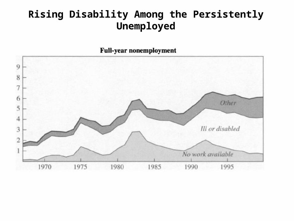
Rising Disability Among the Persistently Unemployed

Autor and Duggan (QJE 2003)

• For a detailed analysis of the intersection of the role of disability andlabor supply, see Autor and Duggan’s:

“The Rise in the Disability Rolls and the Decline in Unemployment”

• Show that during recessions, the disability margin is much more relevantnow than it was during the 1980s (the benefits to the disabled are nowmore comparable to unemployment benefits than before).

Autor and Duggan

More Juhn, Murphy, Topel

Increase in Long Term Non-employment Duration

Increase in Long Term Unemployment Duration

Real Wages Over Time

Unemployment Trends Throughout the Wage Distribution

Nonparticipation Trends Throughout the Wage Distribution

Non-employment Trends Throughout the Wage Distribution

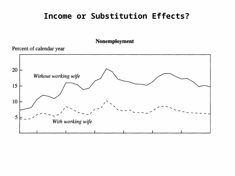
Income or Substitution Effects?

Income of Substitution Effect

Conclusions

• Decline in unemployment rate may not represent accurately the trends in labor market performance.

• Large decline in participation rates for men.

• Non employment has declined much less than unemployment.

• The decline is much more pronounced for low wage men.

• Does it tell us substitution effects are important? What about changes in transfers?

Part C: A Recent Story – Elsby and Shapiro (AER, 2011)

Why Does Trend Growth Affect Equilibrium Employment? A New Explanation of an Old

Puzzle

(Note: I am using some of Elsby’s slides)

Existing Explanations

• Juhn, Murphy, and Topel (1991, 2002) suggest decline in demand for low-skilled labor in 1970s and 1980s.

• Autor & Duggan (2003), Bound & Waidmann (1992) suggest increase in generosity of disability insurance accounts for declines in employment rates among older men (45+).

Our Contribution

• We emphasize the role of wage growth in reducing work incentives through 2 channels:

a) Reductions in the returns to experience among low-skilled workers; and

b) Reductions in the rate of aggregate wage growth that accompanied the productivity slowdown.

Preview of Findings

Given observed trends in wage growth we find that the model can account for:

a)Most of the long run rise in nonemployment among high school dropouts.

b)One half of the rise in economy-wide nonemployment.

c)The observed age structure of these effects.

The Basic Idea

Consider the following simple problem:

• Infinitely lived worker

• Once-and-for-all decision at start of working life between:a) Working forever; and

b) Not working forever.

• What is the optimal labor supply policy?

The Decision to Work

Work Forever• Accumulate experience, x• Payoff:

Not Work Forever• Do not accumulate x• Payoff:

• Present value:

lnbt lnb0

gbt

• Present value:

PVwork w0, tr gw gx

PVnot work btr gb

ln wx, t ln w0, 0

gwt Agg. Growth

gxx Return to Exp.

The Reservation Wage

It follows that the worker will choose to work if:

w0, t wRt bt

where: r gw gx

r gb

Steady State EmploymentImagine an economy populated by workers facing different

wages,

wix, t iwx, t, where i is “skill”

and different payoffs from nonemployment,

bit ibtThen, aggregate employment is given by:

L Prwi0, t bit 1

where Ω = c.d.f. of ω/β & ρ = replacement rate (bi/wi).

Implications of Simple Model

1. [Well understood.] Increases in ρ, the replacement rate, reduce L*.

2. In the long run, it must be that gb = gw.

Otherwise, ρ = b(t)/w(0,t) → 0 or ∞, and L* → 0 or 1 in the limit.

Thus, r gw gxr gb

1 gxr gw

L 1


3. Increases in the return to experience gx reduce α and raise aggregate employment.

– gx > 0 drives reservation wage below payoff from nonemployment.

– Future returns to work forgo current earnings.– Increases in gx reduce res. wages still further.

– Effect will be powerful since r – gw likely small.

L 1 1 gxr gw


4. Increases in aggregate wage growth gw reduce α and raise aggregate employment, IFF gx > 0.

– Increases in gw have a greater impact on PV of earnings for those in work—they compound the return to experience.

– N.B. this effect is absent if gx = 0!

Relates to Blanchard’s neutrality critique:

when gx = 0, gw is neutral w.r.t. employment.

L 1 1 gxr gw

A More General Model

Simple model introduced before, while intuitive, is very stylized in a number of ways:

• Once-and-for-all labor supply decision.• Linear return to experience.• Infinite lifetimes.

To get a sense of the quantitative implications of the model, we now relax these restrictions.

Summary of Qualitative Predictions

a) Increases in the return to experience stimulate employment.

b) If there is a positive return to experience, increases in aggregate wage growth also stimulate employment.

c) These effects are strongest among low-skilled who are marginal to employment decision.

Evidence

We now present evidence on these two forms of wage growth for the US:

• Changes in the return to experience among low-skilled;

• Changes in aggregate wage growth.

Changes in the Return to Experience

Data from 1960–00 Censuses and 2001–07 ACS

Earnings: Annual wages and salary.

Education: dropouts (9-11 yrs), high school, some college, college+.

Experience: Age – education – 6.

Sample: Full-time, full-year non-immigrant white males.

0

0.25

0.5

0.75

1

1.25

1.5

1.75

2

0 10 20 30

Log

Earn

ings

, Nor

mal

ized

Potential Experience, Years

A. 9-11 Years of Education

1960 1970 1980

1990 2000 2001-07

0

0.25

0.5

0.75

1

1.25

1.5

1.75

2

0 10 20 30

Log

Earn

ings

, Nor

mal

ized


B. 12 Years of Education

1960 1970 1980

1990 2000 2001-07

0

0.25

0.5

0.75

1

1.25

1.5

1.75

2

0 10 20 30

Log

Earn

ings

, Nor

mal

ized


D. 16+ Years of Education

1960 1970 1980

1990 2000 2001-07

Sensitivity

1. Actual vs. Synthetic Cohorts– Similar picture.

2. Potential vs. Actual Experience– Effects likely to be small.

3. Selection– Hard to generate flattening profile.

4. Relation to Existing Literature– Similar picture using different data/methods.

Cohort Earnings Profiles: A Similar Pattern

0

0.25

0.5

0.75

1

1.25

1.5

1.75

2

0 5 10 15 20 25 30

Log

Earn

ings

, Nor

mal

ized


A: 9-11 Years of Education

1960 1970 1980

1990 2000

Summary

This paper (hopefully) has:

• Provided an analytical framework in which the labor supply effects of wage growth can be understood.

• Documented the substantial decline in the returns to experience among low-skilled workers.

• Demonstrated that the employment effects of reduced returns to experience and aggregate wage growth are potentially substantial.

Erik’s Comments

Do not allow bi to differ by group

o Value of leisureo Transfer policy

Conduct all analysis using pre-tax dollars

o Do not allow for changes in Tax policy

Assumes changes in wage profile are known ex-ante

o Is that realistic?

Part D: Some Work in Progress

Aguiar, Hurst, and Karabarbounis (in progress)

• Calibrate preference parameters for labor supply (and potentially home production and leisure production function parameters) given:

o Observed hours/participation for different skill groupso Observed home production time for different skill groupso Observed wages for different groupso Observed prices of home production, leisure, and other goodso Observed taxes and transfers for different groups

• Goal:

o To match both the time series and cross sectional trends

• Focus on a group where disability is much less of a concern.

Part E: Unemployment in Current Recession

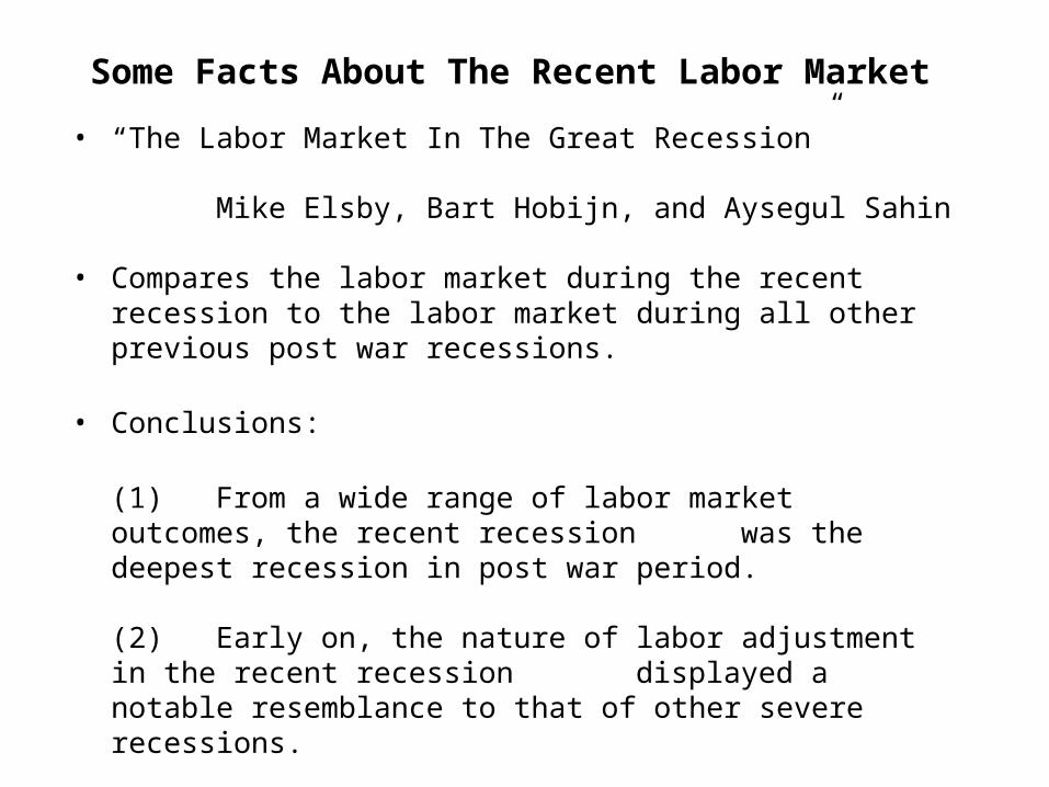
Some Facts About The Recent Labor Market

• “The Labor Market In The Great Recession”

Mike Elsby, Bart Hobijn, and Aysegul Sahin

• Compares the labor market during the recent recession to the labor market during all other previous post war recessions.

• Conclusions:

(1) From a wide range of labor market outcomes, the recent recession was the deepest recession in post war period.

(2) Early on, the nature of labor adjustment in the recent recession displayed a notable resemblance to that of other severe

recessions.

(3) During the latter part of recession (and recovery), the path of adjustment exhibited important departures from other deep recessions.

2008Q12008Q2

2008Q3

2008Q4

2009Q1

2009Q22009Q3

2009Q42010Q12010Q22010Q32010Q4

-6

-4

-2

0

2

4

6

-10 -8 -6 -4 -2 0 2 4 6 8

Source: Bureau of Economic Analysis, Bureau of Labor Statistics, and Congressional Budget OfficeOutput gap

Unemployment gap

No recessionRecessions

Figure 3. Okun’s Law, 1949-2010 Q4

Elsby/Hobijn/Sahin/Valletta 9/16/2011

Labor Market In the Great Recession: An Update

70

Revisions led to partial reversal Okun’s Law

2011Q2

-4

-3

-2

-1

0

1

2

3

4

5

6

-10 -8 -6 -4 -2 0 2 4 6

Source: Bureau of Economic Analysis, Bureau of Labor Statistics, Congressional Budget Office, FRBSF staff

Based on CBO potential output and NAIRU estimates (1949Q1-now)

Okun's Law

Output gap

Unemployment gap

2007 Recessionand after



72

Recent drop in unemployment through participation

62

63

64

65

66

67

68

0

2

4

6

8

10

12

1990 1995 2000 2005 2010Source: Bureau of Labor Statistics

Monthly observations; seasonally adjustedUnemployment and Labor Force Participation rates

Percent Percent

Unemployment rate

Labor force participation rate

2

4

6

8

10

12

1990 1993 1996 1999 2002 2005 2008 2011

2

4

6

8

10

12

Unemployment Rate by Gender

Source: Bureau of Labor Statistics

Women

Men

Unemployment Rate Unemployment RateSeasonally Adjusted

Oct

200

9

2.7

1.1

0.1

0.15

0.2

0.25

0.3

1990 1994 1998 2002 2006 2010

0.1

0.2

0.3

0.4

Unemployment to Non-Participation by Gender


Men

Percent Men

Seasonally Adjusted

Percent Women

Women

0.1

0.2

0.3

0.4

1990 1994 1998 2002 2006 2010

0.1

0.2

0.3

0.4

Unemployment to Employment by Gender


Men

PercentSeasonally Adjusted

Percent

Women

0

0.01

0.02

0.03

1990 1994 1998 2002 2006 2010

0

0.01

0.02

0.03

Employment to Unemployment by Gender


Men


Percent

Women

0

0.01

0.02

0.03

0.04

0.05

1990 1994 1998 2002 2006 2010

0

0.01

0.02

0.03

0.04

0.05

Nonparticipation to Unemployment by Gender


Men


Percent

Women



78

Change in Unemployment RatesTable 1: Change in Unemployment Rates (ppt)

Recession Recovery

Change in Unemployment Rate 5.5 -0.9Gender

Male 6.5 -1.6Female 4.3 -0.2

Age16-24 8.8 -1.625-54 5.4 -0.955+ 4.0 -0.3

EducationLess than High Scool 8.3 -0.6High School 6.5 -1.0Some College 5.3 -0.9College or Higher 2.9 -0.4

RaceWhite 5.2 -1.1Black 7.5 0.3Hispanic 7.2 -1.1

Notes: The recession refers to 2007Q2 to 2009Q4 and the recovery 2009Q4 to 2011Q2

The Unemployment Rate By Skills: All (20-45)

Education2007

UnempRate

2011Unemp

Rate

Change in

Rate

Share of

Pop.

Share Weighted

Change

Percent of Total

Unemp Rate

Explained

High School or Less

7.1% 15.2% 8.2% 41% 3.3% ~65%

Some College 4.2% 8.9% 4.7% 30% 1.5% ~25%

College or More

1.9% 4.5% 2.6% 29% 0.7% ~10%

All 4.6% 9.9% 5.3%

The Non Participation Rate By Skills: All

Education2007

Non-EmpRate

2011Non-Emp

Rate

Change in

Rate

Share of

Pop.

Share Weighted

Change

Percent of Total

Non-EmpRate

Explained

High School or Less

22.1% 24.1% 2.0% 41% 0.8% ~50%

Some College 19.0% 21.8% 2.8% 31% 0.9% ~50%

College or More

12.1% 12.2% 0.1 29% 0% 0%

All 18.4% 19.9% 1.5%

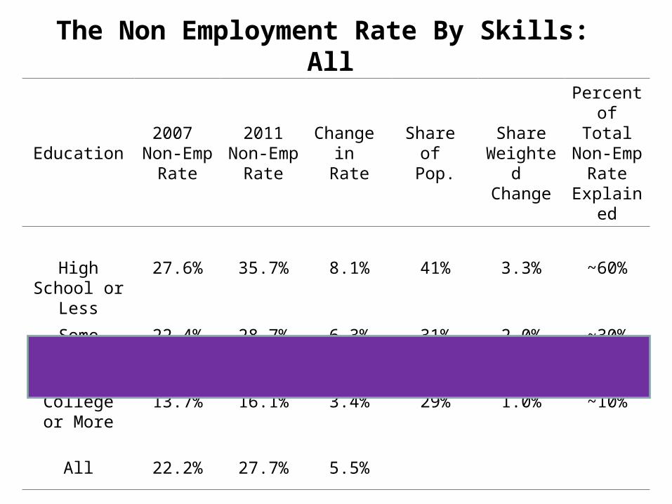
The Non Employment Rate By Skills: All

Education2007

Non-EmpRate

2011Non-Emp

Rate

Change in

Rate

Share of

Pop.

Share Weighted

Change

Percent of Total

Non-EmpRate

Explained

High School or Less

27.6% 35.7% 8.1% 41% 3.3% ~60%

Some College 22.4% 28.7% 6.3% 31% 2.0% ~30%

College or More

13.7% 16.1% 3.4% 29% 1.0% ~10%

All 22.2% 27.7% 5.5%



84

Long-term Unemployment Still High

0

2

4

6

8

10

1994 1995 1996 1997 1998 1999 2000 2001 2002 2003 2004 2005 2006 2007 2008 2009 2010 2011

79 weeks and over

52-78 weeks

26-52 weeks

15-26 weeks

5-14 weeks

<5 weeks

Source: Bureau of Labor Statistics, Current Population Survery, and authors' calculations

Seasonally adjusted monthly observationsUnemployment rate by duration

Percent

Unemployment Duration



86

Historically Low Outflows Even After Recession

0.0%

1.0%

2.0%

3.0%

4.0%

5.0%

6.0%

0%

20%

40%

60%

80%

100%

120%

1948 1953 1958 1963 1968 1973 1978 1983 1988 1993 1998 2003 2008Source: Bureau of Labor Statistics and authors' calculations

Monthly hazard based on Shimer (2005); 3-month moving averagesFlow hazard rates into and out of unemployment

Outflow hazard Inflow hazard

Outflow hazard, f(t)

Inflow hazard, s(t)



87

Pick-up in Outflows to Non-participation

0

5

10

15

20

25

30

35

40

1967 1972 1977 1982 1987 1992 1997 2002 2007Source: Shimer (2007), based on Ritter data provided by Hoyt Bleakley, Bureau of Labor Statistics, authors' calculations

Seasonally adjusted; 3-month moving averageOutflow rates out of unemployment by destination

Percent of unemployed

To Employment

To Non-participation



88

Outflow Rates by Duration and Destination

0

10

20

30

40

50

60

1 2 3 4 5 6 7 8 9 10 11 12 13 14 15 16 17 18 19 20 21 22 23 24+

Source: Current Population Survey and authors' calculations

Average July 2010 - June 2011Monthly outflow rates out of unemployment

Duration (months)

Percent

Total

to employment

to out of the labor force



89

Very High Inflows from Non-participation

0

0.5

1

1.5

2

2.5

1967 1972 1977 1982 1987 1992 1997 2002 2007Source: Shimer (2007), based on Ritter data provided by Hoyt Bleakley, Bureau of Labor Statistics, authors' calculations

Seasonally adjusted; 3-month moving averageInflow rates into unemployment by origin

Percent of labor force

From Employment

From Non-participation



90

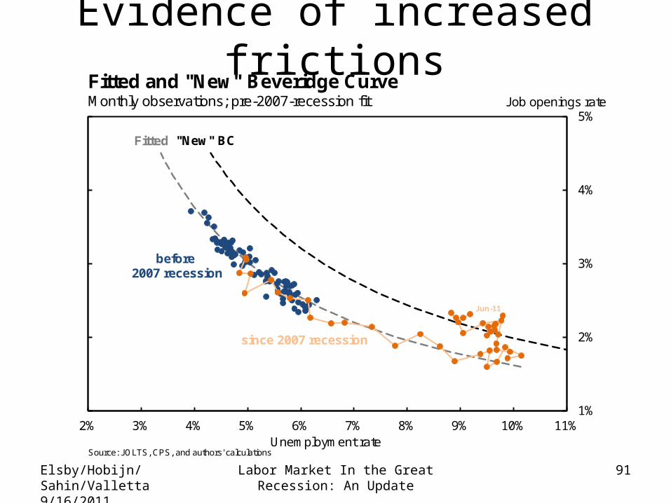
Evidence of increased frictions

Jun-11

1%

2%

3%

4%

5%

2% 3% 4% 5% 6% 7% 8% 9% 10% 11%

Source: JOLTS, CPS, and authors' calculations

Monthly observations; pre-2007-recession fitActual and fitted Beveridge Curve

Unemployment rate

Job openings rate

before 2007 recession

since 2007 recession

Fitted

Gap: 2.6%



91

Evidence of increased frictions

Jun-11

1%

2%

3%

4%

5%

2% 3% 4% 5% 6% 7% 8% 9% 10% 11%

Source: JOLTS, CPS, and authors' calculations

Monthly observations; pre-2007-recession fitFitted and "New" Beveridge Curve

Unemployment rate

Job openings rate

before 2007 recession

since 2007 recession

Fitted "New" BC



92

Broadbased decline in finding rates

0

0.1

0.2

0.3

0.4

0.5

0.6

0.7

0.8

2000 2001 2002 2003 2004 2005 2006 2007 2008 2009 2010 2011Source: Bureau of Labor Statistics and authors' calculations

12-m moving averages of monthly dataUnemployment Outflow Hazards by Industry

Monthly outflow hazard

Total

Construction

Durable GoodsInformation

Financial

Part F: Long Run Trends And Current Recession

Interactions

Where Are Potential Long Term Unemployment Forces Coming From

1. Economic boom from the late 1990s through the mid 2000s

o Housing boom

o Credit boom

2. Persistent decline in manufacturing over last 30 years.

Note: These two forces could have important interactions.

Background: Male Labor Force Participation Rate (All)

Share of “Prime Age” Men Working in Manufacturing

Rise of China: Autor et al. (2011)

Share of Prime Age Men Out of the Labor Force

Share of Prime Age Lower Educated Men Working in Manufacturing

Share of Prime Age Lower Educated Men Out of the Labor Force

Some More Conclusions

• Manufacturing has been steadily declining over past few decades.

• The decline has been felt most by lower educated men.

• The decline has been associated with an exit of lower educated men from the labor force.

House Price Growth

Share of Prime Age Men Working in Construction

Share of Prime Age Low Educated Men Working in Construction

Interaction Between the Construction and Manufacturing: Low Educated Men

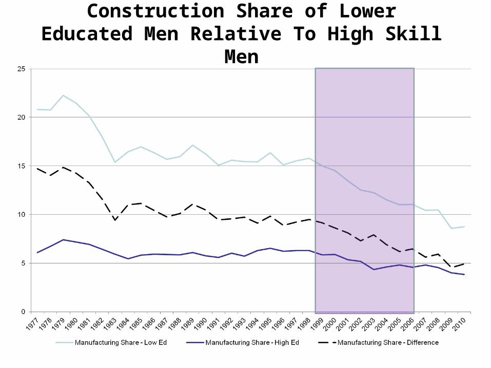
Construction Share of Lower Educated Men Relative To High Skill Men

Out of Labor Force of Low Skill Men Relative to High Skill Men

Wages of Lower Educated Men

Labor Market Break Down of Younger Low Educated (<= 12)Men

Labor Market Status 1997 2007 2010

Out of Labor Force 10.7 12.5 13.9

Unemployed 7.3 6.6 16.0

Construction 13.6 18.8 13.1

Manufacturing 15.5 11.0 8.8

Other 52.1 51.1 48.2

Incarceration Rate about 5% in 2010.

Labor Market Break Down of Younger High Educated (>= 16) Men

Labor Market Status 1997 2007 2010

Out of Labor Force 4.2 5.0 5.6

Unemployed 1.9 1.6 4.7

Construction 1.9 2.4 1.5

Manufacturing 2.1 1.9 1.7

Other 89.9 89.1 86.8

A Potential Hypothesis About Current Unemployment

• The decline of manufacturing would have gradually caused an exodus of low skilled men from the labor market.

• Decline in manufacturing puts downward pressure on wages of low skilled men.

• During previous two decades, such forces was associated with an exodus of low skilled men out of the labor force.

• During the past decade, the housing (construction) boom may have delayed the inevitable (giving low skill men another employment option)

• As construction returns to “normal” and manufacturing has disappeared, what will low skill men do?

• May transition through unemployment before exiting the labor force.

Lecture 4: Time Series and Business Cycle Patterns in Labor Supply

Documents

Transcript of Lecture 4: Time Series and Business Cycle Patterns in Labor Supply