WHY DO RURAL FIRMS LIVE LONGER? 

 Li Yu, Peter F. Orazem, Robert Jolly 

Working Paper No. 09013 July 2009  

IOWA STATE UNIVERSITY Department of Economics Ames, Iowa, 50011‐1070 

Iowa State University does not discriminate on the basis of race, color, age, religion, national origin, sexual orientation, gender  identity, sex, marital status, disability, or status as a U.S. veteran.  Inquiries can be directed  to  the Director of Equal Opportunity and Diversity, 3680 Beardshear Hall, (515) 294‐7612. 

WHY DO RURAL FIRMS LIVE LONGER?

Li Yu

Peter F. Orazem

Robert Jolly

July, 2009

Abstract Rural firms have a higher survival rate than urban firms. Over the first 13 years after firm entry, the hazard rate for firm exits is persistently higher for urban firms. While differences in firm attributes explain some of the rural-urban gap in firm survival, rural firms retain a survival advantage 18.5% greater than observationally equivalent urban firms. We argue that in competitive markets, the remaining survival advantage for rural firms must be attributable to unobserved factors that must be known at the time of entry. A plausible candidate for such a factor is thinner markets for the capital of failed rural firms. The implied lower salvage value of rural firms suggests that firms sorting into rural markets must have a higher probability of success in order to leave their expected profits equal to what they could earn in an urban market. JEL: O18, L21, D92 Key words: Rural, urban, entry, exit, survival, sorting , salvage value We gratefully acknowledge financial support from the Iowa State Agricultural Entrepreneurship Initiative. This journal paper of the Iowa Agriculture and Home Economics Experiment Station, Ames, Iowa, Project No. IOW03804, was supported by hatch Act and State of Iowa funds. Corresponding author is Li Yu, Department of Economics, Iowa State University, Ames, IA 50011-1070, Email: yuli@iastate.edu , Phone: (515) 294-6042.

2

I. Introduction

Entrepreneurship is increasingly being identified as a key determinate of future

economic growth.1 In turn, the growth only occurs if the pace of entrepreneurial entry

exceeds the rate of firm exits. Even areas with relatively slow firm birth rates may

experience economic expansion if local firms survive and grow. That simple

observation turns out to have key implications for rural economic development: rural

areas experience lower rates of firm entry. Less well known is that rural firms also

have lower rates of firm exit. Understanding the conditions that lead to great rural

firm survival relative to their urban counterparts is critical to understanding rural

economies can grow.

Economists have long established that business survival is influenced by firm

and industry characteristics.2 More recently, economists have also begun to examine

whether business location matters for business survival. Fritsch et al (2006) and Falck

(2007) found that regional characteristics play an important role in business success.

However, little is known about the relative success of rural firms and urban firms.

Figure 1 illustrates the stylized facts that motivate this study: that rural economies

are characterized by slow rates of both firm entry and firm exit. We plot firm entry

and exit rates in the five most rural and the five most urban states in the US. The rural

states consistently have lower firm entry rates than urban states. Less well known is

1 See Acs and Armington, Acs et al (2008), Atudretsch et al (2006), and Baumol et al (2007) for recent examples of this literature. 2 Examples include Audretsch (1991), Audretsch and Mahmood (1995), Esteve-Pérez and Maňez-Castillejo (2008), Mata and Portugal (1994), and Taylor (1999).

3

that rural states also have lower firm exit rates than the urban states. 3,4 However, in

almost all years, the rural firm exit rate is lower than the rural firm entry rate, and so

we have net additions of rural firms.5 Understanding the reasons behind the lower

exit rate of new firms in rural areas may identify factors that ultimately can increase

entrepreneurial activity and economic growth in these regions.

Urban establishments should have numerous advantages over their rural

counterparts. Urban markets are characterized by knowledge spillovers across firms

and workers, a large customer base, easy access to information on new technologies,

easy availability of differentiated skills in the labor markets, close proximity to

suppliers, and superior transportation, telecommunication, and energy infrastructure.

Such advantages have been shown to give urban firms a better chance at survival in

West Germany, for example (Falck, 2007).

However, it is not obvious that all factors favor urban firm survival.

Agglomeration economies in urban areas may be offset by higher input costs such as

wages and rents or by having to face a large number of competitors (Arenius and

Clercq, 2005). For example, Fritsch et al (2006) found that survival rate of newly

founded businesses is negatively related with population density in West Germany.

Bresnahan and Reiss (1990, 1991) found evidence that in the smallest populated

markets, firms can charge monopoly prices. As community population rises, firm

3 Davis et al (2008) argue that the churn rate—the combined pace of firm entry and exit, is systematically related to growth by raising the pace of productivity advances. 4 Plummer and Headd (2008) also found that rural firm death rates are significantly lower than urban firm death rates, but their reported differences were very small. 5 We get similar patterns when we replicate the graph with the ten most and least rural states, but the urban-rural entry and exit rates are more similar.

4

entry quickly drives pricing power to the competitive level.

Our analysis of firm survival in rural and urban regions uses Iowa as a case study.

The data are particularly suited to address why rural firms live longer. Iowa’s 99

counties range from predominantly rural to metropolitan, providing a suitable range of

markets to study this issue. The data set focuses on the universe of nonagricultural

firms that opened for business in 1992 which holds constant the macroeconomic

conditions that prevailed at the time of firm entry. The data is longitudinal which

allows us to follow the firms for 13 years. Because two-thirds of U.S. firms fail

within 6 years, the period is suitably long to establish whether any differences in

survival are permanent or transitory. By holding industry and firm age fixed, we can

measure the rural advantage holding constant differences in industry life cycle

(Agarwal and Gort, 1994) and opportunities for learning-by-doing (Jovanovic and

Lach, 1989). We can also hold fixed regional characteristics, observed and

unobserved firm attributes, and factors influencing the strength of the local and

industry markets.

In addition, the Iowa data mimic the national pattern of higher rural firm survival

rates. Figure 2 shows the proportion of Iowa urban and rural firms that are still in

business six years after entry. Seven firm birth-year cohorts are presented, and in all

but one, rural firms have a higher survival rate after six years. The higher rural

survival rate occurs despite the fact that the Iowa urban firm survival rate is already

higher than the national average.

We find that both rural and urban firms face concave exit rates with peak exits at

5

about 5 years. Over the first 13 years after entry, the hazard rate for firm exits is

persistently higher for urban firms. Even after controlling for differences in firm,

local market and industry factors between urban and rural firms, the rural firms retain

a survival advantage over urban firms. The remaining advantage to rural firms is

attributable to differences in unobserved, time invariant attributes that exist at the time

the firm is born. We argue that the source of this survival advantage is plausibly found

in thinner markets for capital in rural areas that lead to a lower salvage value for failed

rural firms. Because firms have to take the possibility of failure into account at the

time of entry, rural firms must have a higher probability of success in order to leave

expected profits equal across rural and urban markets.

II. The Iowa Longitudinal Firm Database

We require longitudinal data on firms from date of entry to exit. Such data are

available from the National Establishment Time-Series (NETS) database. NETS is a

long-term project of Walls & Associates in conjunction with Dun and Bradstreet

(D&B). The NETS database identifies each establishment using a unique DUNS ID

number6. We use the earliest available Iowa NETS cohort, which includes the

universe of establishments born in Iowa in 1992. If an establishment exits in any year

between 1992 and 2004, excluding the cases where the firm migrates to another

county inside or outside Iowa, it is designated as failing to survive. The sample is

right censored in 2005 consequently all of the remaining establishments survived at

6 The observation unit in the NETS database is the establishment, which might be a stand-alone firm; one of several branches of a multi-plant firm, or the headquarters of a multi-plant firm. The link between subsidiary establishment and parent firm can be identified, and so we can distinguish the performance of branches and subsidiaries from the performance of independent establishments.

6

least thirteen years.

An advantage of the NETS database is that it provides detailed information on

each establishment’s characteristics at the time of firm birth. This information allows

us to control for factors that have been shown to be important in explaining business

survival such as firm ownership and firm size (Audretsch and Mahmood, 1995,

Mahmood, 2000), but at the time of entry rather than later in the firm life cycle. This

side-steps difficulties caused by time varying firm attributes that change

endogenously as each firm’s path toward survival or death progresses. We also have

an unusually long time series on each firm, allowing us to follow firms for more than

twice the median life of firms in the United States.7

Address information on each firm is used to identify the firm’s county of

residence which we take to be its primary consumer market. We also use the county

designation to merge additional county-level data that measures local market

conditions, natural amenities and other characteristics.

The categorization of firms by industry in the NETS database initially used eight

digit Standard Industrial Classification (SIC) codes. During the period covered by this

study, the Census Bureau switched to the North American Industry Classification

System (NAICS). Walls & Associates provides a one-to-one projection table which

translates the SIC codes into NAICS codes which allowed us to place each firm into

consistent two-digit NAICS codes that spanned the full period between 1992 and

2004.

7 See Knaup and Piazza (2007) for U.S. firm survival rates.

7

Looking ahead to our analysis, in 1992, 11,922 firms opened for business in Iowa.

After six years, 64% of rural firms and 61% of urban firms were still in business. By

2005, the end of our sample period, 5,176 firms were still operating, 43 percent of the

1992 entry cohort. Only 40% of urban establishments were still alive compared to 45%

of the rural firms. The difference in average survival rates between urban and rural

areas is statistically significant, and as we saw in Figure 2, is a regular finding for

other entry cohorts. We focus on the 1992 firm entry cohort because it affords us the

longest time period over which to observe firm success or failure. Of course, the

difference in rural-urban firm survival may reflect systematic differences in the types

of firms found in those markets, and so we require a more structured analysis to see

whether rural firms really have a higher rate of survival.

III. Survival Model

The survival duration of an establishment is defined as a random variable T. The

hazard function, representing the probability of exit during a time interval tt Δ+ ,

conditional on the establishment being in business at time t is:

)(/)(

)()()|(lim)(

0 tSttS

tStf

ttTttTtPth

t

∂∂−==

Δ≥Δ+<<

=→Δ

, (1)

where )(tf is the density function and )(tS is the survival function. Figure 3 shows

the non-parametric estimated hazard curves for our 1992 cohort of Iowa

establishments in both rural and urban areas. The curves have an inverse U shape.

While some studies found that hazard rates fell monotonically with establishment age

(Fritsch, Brixy and Falck(2004), Audretsch(1991), and Evans(1987)), more recent

empirical studies have found a concave hazard rate pattern (Mahmood, 2000; Falck,

8

2007). The bell-shaped hazard function suggests a log-logistic distribution in the

accelerated failure time model8 .

We allow firm i’s survival duration T to vary with covariates ix according to the

survival function

γϕγβ /1)(1

1),,(ii

i ttS

+= (2)

where )exp( βϕ ii x−= , β is a 1×p vector of regression parameters and 0>γ is an

ancillary parameter to be estimated and ix is a 1×p characteristics vector, including

the firm’s own characteristics, location attributes and industry characteristics. If

jβ >0 pj ...,,2,1= , an increase in one of the covariates ijx , holding other covariates

constant, will result in a decelerated or degraded failure which indicates an increased

survival likelihood. In contrast, jβ <0, indicates an accelerated failure or decreased

survival likelihood attributed to the covariate, all else equal.

Homogeneous risk of firm failure

The parameter γ in equation (2) influences the shape of survival and hazard

functions. When γ >1, the hazard rate is monotonic in duration. If 0<γ <1, the

estimated hazard rate will first increase and then decrease with time, as found in the

8 The log-logistic model fits the data well. Our conclusion is based on a common diagnostic tool that plots the Cox-Snell residuals against the cumulative hazard function. (Klein and Moeschberger, 1997). If the model is appropriately specified and fits the data, these residuals should have an exponential distribution with its rate parameter equal to one. The plot is shown in Figure A1 in the Appendix. The plot is very close to the 450 line, indicating the log-logistic distribution is an appropriate assumption. Other parametric functional forms, such as the Weibull, Log-normal, and Gamma were also investigated and rejected because the residuals are not as close to the 450 line as those from the Log-logistic specification, as seen in the Figure A1 In addition, the Cox (1972) proportional semi-parametric hazard model does not fit the data well because the proportional assumptions are violated in general and for nearly half of the covariates included in the estimation.

9

simple nonparametric hazard shown in Figure 3.

Hypothesis 1: 10 << γ in the log-logistic survival model so that firms face a

concave failure hazard rate.

The hazard rate, according to definition (1) is given by

])(1[),,( /1

/11/1

γ

γγ

ϕγϕ

γβii

iii t

tth+

=−

. (3)

The log likelihood is

1 11

n n

i i i i ii i

L( , | x ) d ln f ( t , , ) ( d )ln S( t , )β γ β γ β γ= =

= + −∑ ∑ , (4)

where ),,( γβtf is the probability density function of survival duration T ; and d is a

binary variable, equal to one if the establishment exits from the market.

Heterogeneous risk of firm failure

The model above assumes that each individual establishment is exposed to the

same risk once characteristics ix are controlled. However, there may be unobserved

factors that influence the mortality of establishments. For example, Jovanovic(1982)

assumes firms are heterogeneous in their abilities to learn-by-doing, creating a

mixture of firms that differ in productive efficiency. Over time, the inefficient firms

decline and fail and the efficient firms grow and survive. If the population is a

mixture of individual establishments with different failure risks that are ignored in the

estimation, then the hazard rate tends to be underestimated (Hougaard, 1986, Omori

and Johnson, 1993).

This unobserved heterogeneity is measured by a quantity called frailty of

individual establishments, defined as a new random variableα . It is incorporated

10

into the individual hazard function as ),,()|,,( γβααγβ ii thth ⋅= and

αγβαγβ )},,({)|,,( ii tStS = . We define α to have mean one and varianceθ 9.

Denote )(~ αα g , where )(αg is the density function ofα . This cumulative effect of

α describes individual establishment’s relative exit risk. Establishments with 1>α

are more frail for reasons that are uncorrelated with the covariates xi that are

included in the estimation. Bad draws on α create a permanent increased risk of

failure for the life of the firm, and could reflect bad luck, bad management, poor

technology choices, or any other unmeasured adverse factor. Firms with good α

draws will have 1<α which permanently raises their probability of survival, all else

being equal (Gutierrez, 2002). As time passes, the establishments tend to become

more homogeneous because frail establishments die earlier than robust ones (Vaupel,

et al, 1979).

In theory, any continuous distribution of α supported on the positive numbers

that has mean one and finite variance is allowed. However, the Inverse-Gaussian

distribution or Gamma distribution is the common choice for the purpose of

mathematical tractability. We chose the Inverse-Gaussian distribution, which makes

the population of survivors more homogeneous with the passage of time than does

the Gamma distribution (Hougaard, 1984, Hougaard, 1986)10. This generates the

second hypothesis to be tested:

9 For the purpose of identification, expectation of α is assumed to be one. To be computationally convenient, we require that α is independent of T. 10 Because of the small difference in properties between Gamma and Inverse-Gaussian frailty distribution, we did similar analysis when the heterogeneity is specified to have a Gamma distribution, the results are still consistent with the ones we obtain under the assumption of Inverse-Gaussian frailty distribution.

11

Hypothesis 2: θ ≠0, implying that firms differ in unobservable relative risk of

failure.

If θ =0, there is no heterogeneity across establishments and so the estimation

reduces to the survival function (2) and log likelihood function (4). If θ ≠ 0,

inclusion of frailty is necessary to capture the excess dispersion in firm hazard rates.

The survival function with heterogeneity incorporated is given by

( )⎭⎬⎫

⎩⎨⎧ −−== ∫

∞)](ln[2111exp)()|(),,,(

0 ii tSdgtStS θθ

αααθγβθ , (5)

The log-likelihood with Inverse-Gaussian distributed heterogeneity is the following,

1 1

1

1

1

1

n n

i i i i ii i

n

i i i ii

L( , , | x ) d ln f ( t , , , ) ( d )ln S ( t , , , )

d ln h( t , , ) ( d )ln[ ln S( t , , )]

θ θβ γ θ β γ θ β γ θ

β γ θ θ β γ

= =

−

=

= + −

= − + −

∑ ∑

∑ (6)

where ),,,( θγβθ tf is the corresponding probability density function of ),,,( θγβθ tS .

Under either model specification (4) or (6) , we can also consider the effect of

observable local market characteristics on firm longevity. Factors that have been

identified as contributing to economic growth more generally, such as the education

level of the local workforce, strong local markets for credit or product demand, and

natural amenities, enter the vector ix . That allows us to test our third hypothesis:

Hypothesis 3: Business survival depends on favorable local economic, labor

market and environmental conditions.

Our primary interest is in assessing whether the impact of these local factors on

firm survival differs between urban and rural areas. We can investigate that

possibility by altering how the vector of local factors enters the analysis.

12

Specifically, insert ),exp( ,, RRxRii Rx ββφ −−= −− into equation (2), where R is a

binary variable indicating the establishment is located in a rural county, and Rix

−,

contains all other covariates included in ix except the constant term. If 0>Rβ after

controlling for all other covariates, then rural firms have a higher survival rate. This

allows us to test our fourth hypothesis:

Hypothesis 4: Holding all firm and local factors constant, rural businesses have a

greater survival rate than urban businesses.

IV. Covariates that may influence firm survival

The variables included in the vector ix represent firm, community and industry

characteristics that are believed to affect firm survival. Summary statistics are

presented in Table 1.

1. Individual establishment specific characteristics

The NETS database identifies establishment specific characteristics, such as

initial establishment size and ownership that may influence the likelihood of survival.

The number of employees at time of birth has been hypothesized to raise survival

prospects because larger firms have advantages in raising capital, face better tax

conditions, and are in a better position to recruit qualified labor (Mahmood, 2000).

Innovation rates and technology adoption intensity are found to be positively related

with the survival probabilities of establishments (Audretsch and Mahmood, 1994,

1995, and Mahmood, 2000). Additionally, because large firms tend to adopt more

advanced technologies in the early stage of technology diffusion, they are more likely

to survive than small firms. Finally, the larger sunk costs associated with opening a

13

larger firm implies a higher prior expectation of profitability. Consequently, greater

survivorship may simply reflect sorting on expected profits at time of firm birth

(Frank, 1988).

Establishment size is categorized into three levels: small, medium and large. A

small establishment has no more than five employees. A medium establishment has

six to fifty employees and a large establishment has more than fifty employees. Two

dummy variables, Medium and Large are used, reserving small firms as the base. 75.5%

of new establishments born in Iowa in 1992 are small and 38.6% of small businesses

were still alive in 2005. In contrast, 22% of new establishments are medium sized and

their survival rate is 56.2%, 17.6% higher than small establishments.

A second factor that may affect firm survival is ownership structure (Audretsch

and Mahmood, 1995). Establishments in our dataset can be independent single entities;

a branch or subsidiary of a multi-establishment firm; or the headquarters of a multi-

establishment firm. Branches or subsidiaries are more likely to survive than

independent firms because branches benefit from the experience and reputation of

their parent firm. Of our new business cohort in 1992, 67.6% are independent

establishments and 31.0% are branches.

Finally, a dummy variable Minority indicates whether the owner is a member of

a minority group. Past research has found a positive correlation between minority

status and the probability of setting up new businesses (Lee, et al., 2004) because

minority groups tend to pool various resources to enable new start-ups (Lee, et al.,

2004, Kandel and Lazear, 1992). However, language limitations or social or cultural

14

isolation may limit access to customers, new business opportunities, or new

technologies critical to firm survival prospects (Arenius and Clercq, 2005, Ozgen and

Baron, 2007).

2. Location specific characteristics

The abundance of local labor, capital, information, or material is critical to the

operation of new firms (Stearns, et al 1995). Stable and healthy development of a

local economy should also increase the likelihood that an establishment can survive.

We introduce several factors that represent a firm’s local economic environment. We

treat a county as the local market in which a firm resides. The 99 counties of Iowa are

of roughly comparable size, and so these measures will reflect roughly the same

geographic boundaries surrounding the firm.

Rural is a dummy variable, indicating whether the county is urban or rural. The

USDA estimates that 53% of Iowa’s establishments are located in rural or nonmetro

counties (Rural-Urban Continuum Codes 4-911). Firms in urban areas should face

higher customer demands and lower search costs for information, and should benefit

from lower production costs attributable to agglomeration (Glaeser, et. al, 1992). On

the other hand, social networks that could result in a loyal customer base are stronger

in rural areas (Arenius and Clercq, 2005). Rural firms will also face lower rent, lower

labor costs and less competitive pressure. Previous studies have not established

whether rural firms have different survival prospects. However, Acs and Malecki

(2003) found a higher percentage of high growth firms in smaller Labor Market Areas,

11 http://www.ers.usda.gov/Data/RuralUrbanContinuumCodes/1993/LookUpRUCC.asp?C=R&ST=IA and http://www.ers.usda.gov/briefing/Rurality/RuralUrbCon/.

15

suggesting that rural firms may have some advantages over urban firms.

Higher Education is defined as the percentage of college degree holders in a

county. In the empirical literature of new business survival, local labor quality is

largely neglected. However, establishments can benefit from knowledge spillovers

which create innovations, generate exterior learning-by-doing, reduce searching costs,

and potentially reduce the hazard of failure (Moretti, 2004). At the same time, more

educated residents have more disposable income therefore they will generate higher

and more diversified demand for local products and services.

Local Capital is measured by per capita bank deposits (in $millions) in the county.

The measure is meant to indicate the availability of loanable funds in the local credit

market. While it may seem that credit markets are very efficient at locating and

funding promising ventures, banks could play an important role in disseminating

information on such opportunities in small or isolated market.

Debt measures log of per capita local public debt in a county. This could be

viewed as a measure of expected future tax obligations that must be paid by firms and

residents. Heavier tax obligations lower discretionary income of the customers and

add cost to the firms, both of which may lower the probability of survival. Both Debt

and Local Capital emphasize the effect of liquidity constraints faced by entrepreneurs.

For example, Holtz-Eakin, et al (1994) found that liquidity constraints exerted a

noticeable influence on the viability of entrepreneurial enterprises.

Entry1991 is the entry rate of new businesses in the county in 1991. The variable

is defined as the number of establishments born in the county in 1991 divided by the

16

total number of active establishments in the county in the beginning of 1991. We use

this variable as a correction for selection: we only observe firm exits for firms that

were induced to enter. It is plausible that exit rates are highest in markets that have

the highest firm entry rates, due to low entry costs, or high perceived opportunities.

For example, studies show that imposing barriers to exit such as firing restrictions or

contracted length of service requirements can also serve as a barrier to firm entry in an

industry (Agarwal and Gort, 1994, Eaton and Lipsey, 1980, Macdonald, 1986).

However, it is still not clear if entry costs at a national or regional level affect new

business survival probabilities. If true, then our exit rates will be subject to substantial

selection bias that could cloud our interpretation of the results. If Entry1991

successfully serves as a control for selection, we should find that high values of

Entry1991 will raise the likelihood of exit and lower firm survival.

Amenity is an index from one to seven which represents the quality of natural

amenities in the county. As defined by the Economic Research Service of the USDA,

a higher number means better weather and better access to naturally occurring

topographic or geological features. Water measures the water coverage in a county.

Higher levels of amenity and more water in a county may attract employment and

tourists. Henderson (2007) finds that local growth is enhanced by better amenities and

water coverage in a local region.

Highway is a dummy variable indicating that the county has an interstate highway.

The presence of transportation infrastructure reduces the average cost of production

for firms by reducing distribution costs and input acquiring costs from the distant

17

markets and supports the local employment growth (Henderson, 2007).

3. Sector-specific market growth and industrial structure

A firm should find it easier to survive in a sector with increasing demand. The

market growth variable Growth is measured by the annual percentage change in

employment in the national two digit industry in the four year period between 1998

and 2002, the midpoint of our sample period. Data are compiled from the March

Current Population Surveys from the US Census Bureau. We expect that

establishments are more likely to be viable in industries that are experiencing higher

growth.

Concentration defines the sales percentage of the biggest four firms in a specific

4 digit NAICS coded industry in Iowa in 1991. A high concentration ratio suggests

high entry barriers in the industry. New firms that enter those markets will face

pressures to drop out, even as the older incumbent firms are insulated from competing

with new entrants. One example is in the retail sector where big firms tend to drive

out small firms (Jia, 2008).

V. Empirical Results

Regression results from the survival model specified in equation (6) are shown in

Table 2. Hypothesis 1 cannot be rejected. The estimated shape parameter γ is 0.4 and

statistically significant, supporting our use of the log-logistic specification. This

implies a bell shaped hazard function for firm failures consistent with the patterns

shown in Figure 3.

The variance of the Inverse-Gaussian frailty θ is 2.04 and a likelihood ratio test

18

easily rejects the hypothesis that individual establishments have a homogeneous exit

rate distribution after controlling for the observables. Consistent with Hypothesis 2,

there are significant time-invariant unobserved traits that affect the likelihood of firm

survival. That firms differ in frailty means that over time, firms with bad draws from

the α distribution at time of birth cannot compete and are forced to exit the market.

The process continues until vulnerable establishments are shaken out, and only the

strong establishments with good α draws remain active in the market.

Effects of firm attributes, location, and industry characteristics on survival

From Table 2, we find that survival probability is significantly affected by firm

attributes, local market attributes and industry fixed effects, based on the global tests

on the coefficients of variables in these three categories. Establishments’ own

characteristics significantly affect the survival of new businesses. Consistent with

previous findings, establishments with bigger initial size are less likely to fail than

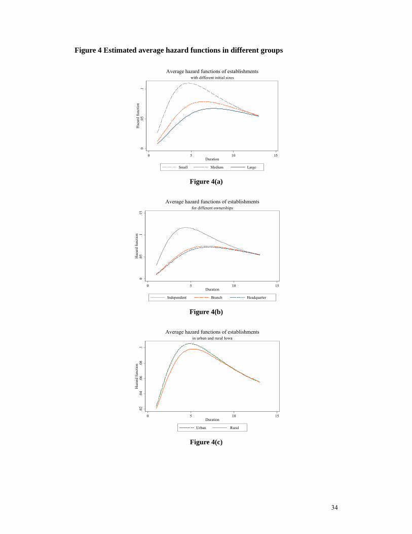
smaller ones. The effect is even stronger for large firms than for medium firms. Figure

4(a) shows that the medium and large establishments have much lower exit hazard

rates than do small establishments. The mortality rate peaks at four to five years for

small establishments. However, the critical duration extends to six to seven years for

medium establishments and to seven to eight years for large establishments. Once

establishments survive eleven years, they are exposed to very similar low mortality

rates, regardless of initial size.

Also consistent with previous findings, establishments born as branches or

subsidiaries are more likely to survive. Headquarters with multiple branches, once in

19

the market, are more likely to survive than independent establishments. Their

estimated hazard functions are shown in Figure 4(b). The maximum mortality for

independent firms peaks at age four. However, the maximum hazard for branches and

headquarters peaks in their seventh year.

Regional factors also influence firm survival, consistent with Hypothesis 3. Firm

survival likelihood is improved in counties with higher proportions of college

graduates and counties with water amenities such as lakes and streams. Firm chance

of survival is lower in counties with high levels of per capita public debt. Other

factors such as local access to loanable funds or highways do not affect firm survival,

nor do other amenities such as weather or topography.12

Firm survival probability is also affected by selection. Firms that enter in

counties with higher entry rates are also more likely to exit. We interpret this as

evidence of sorting on the strength of the local market. In stronger markets, more

marginal firms are willing to enter, and faltering firms are more apt to exit because

they have ready access to new buyers willing to try their hand at entrepreneurship. In

markets with poorer prospects and few entrepreneurs willing to purchase the assets of

the weak, only firms with more certain success will enter.

Firm survival and exit rates differ significantly across industries. Firms survive

more readily in industries with faster growth nationally. Administrative and waste

management establishments have the highest risk of failure, followed by the

entertainment and recreation services and professional services, retail and wholesale

12 There is not much variation across these counties in weather or topography, and so the lack of importance in this application may not hold for samples with greater variation in local amenities.

20

industries.

Rural – urban differentials in survival patterns

Comparing Tables 1 and 2 allow us to identify the factors that help explain the

higher rural firm survival rate. Factors that have a positive effect on survival and

have higher means in rural areas will raise average rural establishment survival.

Factors that lower survival and have lower means in rural areas will also raise average

rural survival rates. The factors that give rural firms a survival advantage are all

factors that lower firm survival: rural areas have lower public debt, lower firm entry

rates, and fewer construction, professional service, administrative service and

arts/entertainment firms. Urban establishments have advantages because they are

larger, more likely to be branches or headquarters, have better access to an educated

workforce and water resources, and atypically are in growing industries.

Even after controlling for all these factors that might explain the differences in

survival rates across urban and rural counties, we cannot reject Hypothesis 4 that

establishments located in rural counties are more likely to survive than those in urban

counties. As shown in Table 2, the rural firms have a 18.5% higher survival

probability that is significant at the 10% level.13 Furthermore, as shown in Figure 4(c),

13 Average survival odds are defined as γβγβ

γβ /1))exp(()|,,(1

)|,,( −−=−

≡ xtxtS

xtSOddsx when α

is held at one. And the corresponding odds ratio between rural and urban firms is

)exp(0

1

γβ R

R

RR Odds

OddsOR ==

=

= =1.185.

21

the failure hazard rate is greater for urban than rural firms for the first nine years after

entry.

Why does a rural firm tend to live longer than an otherwise observationally

equivalent urban firm? It is possible that the attributes included in Table 2 have

different marginal impacts on firm survival in rural compared to urban markets, and

those different marginal effects generate different survival patterns. To test that, we

replicated the estimation strategy used in Table 2 separately for the urban and rural

firms and tested for differences in the coefficients across the urban and rural markets.

We cannot reject the null hypothesis that the firm survival coefficients are the same

across the rural and urban markets, supporting the survival specification used in Table

2.

In competitive markets, a known persistent higher probability of rural firm

survival must be accompanied by a higher cost of rural firm entry in order to leave

expected profits equal at the margin across urban and rural markets. Our remaining

task is to suggest a plausible candidate for the higher rural entry cost. We suggest that

the most likely candidate is a weaker market for the capital of failed rural firms that

lowers the expected salvage value of a rural firm at the time of entry compared to the

salvage value of that same firm in an urban market.

It is commonly known that low population density and poor access to educated

labor, capital and infrastructure deter rural firm entry (Reynolds, et al, 1995). But

those same factors limit the potential market for the plant and equipment of the rural

firms that do enter and subsequently fail. The lower expected salvage value of rural

22

firms at the time of entry implies that rural firms must have a higher probability of

success to justify opening business in the rural rather than in the urban market.

To make a simple example that clarifies the argument, suppose that a firm

considering opening in an urban (U) or rural (R) market has exactly the same expected

revenue and cost stream in both markets. Conditional on survival, assume expected

profit is in both U and R. A firm will only open for business if the expected return

from using capital in operation exceeds the value of that same capital in alternative

uses. Consequently, it must be true that RUjjFS ,, => ππ , where j

Fπ is the salvage

value (or opportunity cost) of the firm’s capital in market j. Suppose that the salvage

value is higher in U, and so RF

UF ππ > . Using jp as the probability of firm success in

region j, we can write expected profit at time of entry as

RUjppE jFjSj ,,)1()( =−+= πππ . If there is free entry into both markets U and R,

)(πE must be the same in U and R, which can only be true if UR pp > . Hence, firms

that sort themselves into rural markets will only do so if they expect a higher survival

probability than they would in an urban market.

We test this sorting hypothesis using a bivariate probit model. Firms jointly

choose whether to enter a rural or urban market in 1992, and whether to stay in

business by 2005. The decisions are based on the observed characteristics included in

Table 2 excluding the location characteristics. We have to exclude the location

characteristics because they are selected jointly with the urban- rural location and are

therefore endogenous.

The error terms include unobserved factors that sort firms into and out of business

23

and into and out of rural markets. If our sorting mechanism is valid, we should find

that the errors are positively correlated: unobserved factors that cause a firm to enter a

rural market (such as low RFπ ) must also raise the likelihood of survival Rp .14

The results are shown in Table 3. The correlation of unobservables contributing to

rural entry and survival is significantly positive, indicating that unobserved regional

attributes that induce rural firm entry also raise the probability of firm survival. The

implication from our hypothesized sorting mechanism cannot be rejected. We also

find that firms that self select into rural areas are small, independent and owned by

non-minority entrepreneurs. These rural firms are more likely to be in competitive

industries. Manufacturing and mining firms, atypically locate in rural areas while

construction, wholesale, finance real estate and professional firms select urban

markets.

VI. Conclusions and discussions

This study uses a unique longitudinal data set to analyze the factors that explain a

previously unexplored phenomenon: the higher survival probability of rural

establishments. We show that across states and across years within states, rural firms

are less likely to exit. As one might expect, many factors actually favor urban firm

survival: urban firms are bigger, have better access to educated workers and water, are

more likely part of a multiplant firm, and are more likely in growing sectors of the

economy. Rural firms have advantages in that they are in markets with a lower public

14 We did add the location characteristics into the survival equation while excluding them from the rural-urban equation to test the robustness of our results. We obtained similar results for the establishment and industry coefficients reported in Table 3. In addition, the critical error correlation estimate was still positive and significant.

24

debt load and lower firm entry rates. Nevertheless, even after controlling for these

characteristics, there remains a significant survival advantage for rural firms that

persist even 13 years after entry.

We argue that a plausible explanation for this persistent survival advantage for

rural firms would be a lower expected salvage value of capital should a rural firm go

out of business. At the time of entry, firms must take into account the possibility that

they will fail and the resources they can still claim in the event they do not survive.

Thin markets for capital in rural areas mean that the same firm will expect lower

salvage value in rural areas which requires a higher probability of success in order to

leave expected profits in rural and urban areas equal. We show evidence that indeed,

unobserved factors that lead a firm to enter a rural market are correlated with higher

firm success, consistent with our presumption that firms self-select into rural markets

based on higher expected likelihood of success.

25

References [1] Acs, Zoltan and Catherine Armington. Employment growth and entrepreneurial

activity in cities. Regional Studies 38 (8): 911 – 27. [2] Acs, Zoltan and Edward Malecki. Entrepreneurship in rural America: the big

picture. Federal Reserve Bank of Kansas City. 2003 [3] Agarwal, Rajshree and Michael Gort. The evolution of markets and entry, exit and

survival of firms. The Review of Economics and Statistics 78(3) 1996: 489-98. [4] Arenius, Pia and Dirk De Clercq. A network – based Approach on opportunity

recognition. Small Business Economics 24(3) 2005: 249-265. [5] Audretsch, David A., Max C. Keilbach and Erick Lehmann. Entrepreneurship and

Economic Growth. New York: Oxford University Press [6] Audretsch, David and Talat Mahmood. The hazard rate of new establishments: A

first report. Economics Letters 36 (4) 1991: 409-412. [7] Audretsch, David and Talat Mahmood. Firm selection and industry evolution: the

post-entry performance of new firms. Journal of Evolutionary Economics 4(3) 1994: 243-260.

[8] Audretsch, David and Talat Mahmood. New firm survival: new results using a hazard function. Review of Economics and Statistics 77(1) 1995: 243-260.

[9] Baumol, William J., Robert E. Litan and Carl J. Schramm. Good capitalism, bad capitalism and the economics of growth and prosperity. New Haven, Yale University Press

[10] Bresnahan, Timothy F. & Peter C. Reiss. “Entry in Monopoly Markets,” The Review of Economic Studies, 57(4) 1990: 531-551.

[11] Bresnahan, Timothy F. & Peter C. Reiss. "Entry and Competition in Concentrated Markets," Journal of Political Economy, 99(5) 1991: 977-1009.

[12] Cox, D. R. Regression models and life-tables (with discussion). Journal of the Royal Statistical Society B (34) 1972.

[13] Davis, Steven J., John Haltwanger and Ron Jarmin. Turmoil and growth: young businesses, economic churning and productivity gains. Ewing Marion Kaufmann Foundation, Kansas City

[14] Eaton, Curtis and Richard Lipsey. Exit Barriers are Entry Barriers: The Durability of Capital as a Barrier to Entry. The Bell Journal of Economics 11(2) 1980: 721-729.

[15] Esteve-Pérez, Silviano and Juan Maňez-Castillejo. The resource-based theory of the firm and firm survival. Small Business Economics 30(3) 2008: 231-249.

[16] Evans, D. S. Tests of alternative theories of firm growth. The Journal of Political Economy 95(4) 1987: 657-674.

[17] Falck Oliver. Survival chances of start-ups, do regional conditions matters? Applied Economics 39(16) 2007: 2039-2048.

[18] Frank, Murray. An intertemporal model of industrial exit. The Quarterly Journal of Economics 103(2) 1988: 333-344.

[19] Fritsch, Michael, Udo Brixy and Oliver Falck. The effect of industry, region and time on new business survival – a multi-dimensional analysis. Review of

26

Industrial Organization (28) 2006: 285-306. [20] Glaeser, Edward, Hedi Kallal, José Scheinkman and Andrei Sheiefer. Growth in

cities. Journal of Political Economy 100(6) 1992: 1126-1152. [21] Gutierrez, Roberto. Parametric frailty and shared frailty survival models. The

Stata Journal 2(1), 2002: 22-44. [22] Henderson, Jason. Understanding rural entrepreneurs at the county level: data

challenges. Federal Reserve Bank of Kansas City – Omaha Branch. October, 2007. [23] Holtz-Eakin, Douglas, Joulfaian, David and Rozen, Harvey. Sticking it out:

Entrepreneurial survival and liquidity constraints. Journal of Political Economy 102(1) 1994: 53-75.

[24] Hougaard, Philip. Life table method for heterogeneous populations: distributions describing the heterogeneity. Biomentrika 71, 1984: 75-83.

[25] Hougaard, Philip. Survival models for heterogeneous populations derived from stable distributions. Biometrika 73(2) 1986: 387-396.

[26] Jia, Panle, What happens when Wal-Mart comes to town: an empirical analysis of the discount industry. Econometrica 76(6) 2008: 1263-1316.

[27] Kandel, E., and Lazear, E. Peer pressure and partnership. Journal of Political Economy 100(4) 1992: 801-817.

[28] Klein, J. P. and M. L. Moeschberger. Survival analysis: Techniques for censored and truncated data. New York: Springer. 1997.

[29] Lee, Sam Youl, Richard Florida and Zoltan Acs. Creativity and entrepreneurship: A regional analysis of new firm formation. Regional Studies 38(8) 2004: 879-891.

[30] Jovanovic, Boyan. Selection and the evolution of industry. Econometrica 50(3) 1982: 649-670.

[31] Jovanovic, Boyan and Lach, Saul. Entry, exit and diffusion with learning by doing. The American Economic Review 79(4) 1989: 690-99.

[32] Knaup, Amy and Piazza, Merissa. Business employment dynamics data: survival

and longevity, II. Monthly Labor review. September, 2007. [33] Macdonald James. Entry and exit on the competitive fringe. Southern Economic

Journal 52(3) 1986: 640-652. [34] Mahmood, Talat. Survival of newly founded businesses: A Log-Logistic model

approach. Small Business Economics 14(3) 2000: 223-237. [35] Moretti, Enrico. Workers' education, spillovers and productivity: Evidence from

plant-level production functions. American Economic Review 94(3) 2004: 656-690. [36] Mata, José and Portugal, Pedro. Life duration of new firms. The Journal of

Industrial Economics 42(3) 1994: 227-245. [37] Omori, Yasuhiro, and Johnson, Richard. The influence of random effects on the

unconditional hazard rate and survival function. Biometrika 84(9) 1993: 910-914. [38] Ozgen, E. and Baron, R. Social sources of information in opportunity

recognition: Effects of mentors, industry networks, and professional forums. Journal of Business Venturing 22(2) 2007: 174-192.

[39] Plummer, Lawrence and Brian Headd. Rural and urban establishment births and deaths using the U.S. Census Bureau’s business information tracking series. An

27

Office of Advocacy Working Paper. February, 2008. [40] Reynolds, Paul, Brenda Miller and Wilbur Maki. Explaining regional variation in

business births and deaths: U.S. 1976-88. Small Business Economics 7 1995: 389- 407.

[41] Stata Manual [ST], Version 8.0. Stata Press. [42] Stearns, Timothy, Nancy Carter, Paul Reynolds and Mary Williams. New firm

survival: Industry, strategy and location. Journal of Business Venturing 10(1) 1995: 23-42.

[43] Taylor, Mark. Survival of the fittest? Analysis of self employment duration in Britain. The Economic Journal. 109(454) 1999: 140-155.

[44] Vaupel, James, Kenneth Manton and Eric Stallard. The impact of heterogeneity in individual frailty on the dynamics of mortality. Demography 16(3) 1979: 439-454.

28

Figure 1 Entry and exit rates in rural and urban states, 1977-2005

Note: The five most rural states include Vermont, Maine, West Virginia, Mississippi, and South Dakota. Average rural population density in these states is 55%. The five most urban states include California, New Jersey, Nevada, Hawaii, and Massachusetts with average rural population density of 7%. Data source: http://www.ces.census.gov/index.php/bds/.

8

10

12

14

16

18

20

1975 1980 1985 1990 1995 2000 2005R‐Entry Rate R‐Exit Rate U‐Entry Rate U‐Exit Rate

29

Figure 2: Iowa urban and rural 6-year firm survival rates by year of startup

65.570.7

47.5

63.6

52.2 54.3

45.3

61.4

68.3

41.9

58.0

45.149.7 49.3

0

10

20

30

40

50

60

70

80

1992 1993 1994 1995 1996 1997 1998

Rural UrbanEntry  cohorts by year

Figure 3 Estimated non-parametric hazard rate function for firm exits, by firm location

Note: log-rank test of equality in survival functions between rural and urban firms is rejected at 1% level( 56.28)1(2 =χ ).

.0

.04

.06

.08

.1

0 5 10 15Duration

Smoothed estimated hazard function

Rural exit rates

Urban exit rates

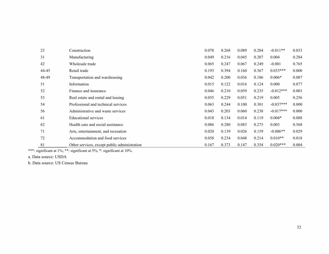
Table 1 Descriptive statistics of variables and definitions.

Variable Description Rural Urban Difference p-value

Mean Std. D Mean Std. D (rural-urban)

Survival duration T Life of establishments 9.069 4.231 8.694 4.234 0.376*** 0.000

Establishment characteristics

Minority 1 if the owner is from a minority, 0 otherwise 0.001 0.038 0.005 0.069 -0.003*** 0.001 Medium 1 if number of employees in the establishment is between 6 and 50, 0 otherwise 0.198 0.398 0.242 0.428 -0.045*** 0.000

Large 1 if number of employees in the establishment is more than 50, 0 otherwise 0.020 0.140 0.029 0.169 -0.009*** 0.001 Branch 1 if the establishment is a branch of a multi-establishment firm, 0 otherwise 0.294 0.456 0.322 0.467 -0.028*** 0.001

Headquarters 1 if the establishment is the headquarter, 0 otherwise 0.012 0.110 0.017 0.128 -0.004** 0.045 Location characteristics

Education a The proportion of residents with a at least college degree in the county 13.594 5.852 21.572 6.935 -7.978*** 0.000 Local Capital a The per capita deposits in the county in 2003 17.873 4.343 17.844 7.003 0.029 0.786

Debt a Log (debt in 1997 / population in 2000) in a county -0.027 0.591 0.516 0.343 -0.543*** 0.000 Entry1991 The entry rate in the county where the establishment is located 0.026 0.007 0.043 0.010 -0.017*** 0.000

Amenities a Natural amenities scale(1-7 with 7 meaning most natural amenities) 2.345 0.495 2.538 0.499 -0.193*** 0.000 Water a Percentage of water areas in a county 0.849 1.194 1.834 1.314 -0.986*** 0.000

Highway a 1 if the county is close to a highway, 0 otherwise 0.259 0.438 0.945 0.227 -0.687*** 0.000 Industry characteristics

Growth b The annual percentage change in employment in US industries 1.527 1.583 1.671 1.597 -0.144*** 0.000 Concentration Concentration ratio of the four largest firms in 4-digit NAICS industries 0.232 0.267 0.238 0.225 -0.006 0.224

21 Mining 0.002 0.042 0.001 0.027 0.001 0.111

32

23 Construction 0.078 0.268 0.089 0.284 -0.011** 0.033 31 Manufacturing 0.049 0.216 0.045 0.207 0.004 0.284

42 Wholesale trade 0.065 0.247 0.067 0.249 -0.001 0.765 44-45 Retail trade 0.193 0.394 0.160 0.367 0.033*** 0.000

48-49 Transportation and warehousing 0.042 0.200 0.036 0.186 0.006* 0.087 51 Information 0.015 0.122 0.016 0.124 0.000 0.877

52 Finance and insurance 0.046 0.210 0.059 0.235 -0.012*** 0.003 53 Real estate and rental and leasing 0.055 0.229 0.051 0.219 0.005 0.256

54 Professional and technical services 0.063 0.244 0.100 0.301 -0.037*** 0.000 56 Administrative and waste services 0.043 0.203 0.060 0.238 -0.017*** 0.000

61 Educational services 0.018 0.134 0.014 0.119 0.004* 0.088 62 Health care and social assistance 0.086 0.280 0.083 0.275 0.003 0.568

71 Arts, entertainment, and recreation 0.020 0.139 0.026 0.159 -0.006** 0.029 72 Accommodation and food services 0.058 0.234 0.048 0.214 0.010** 0.018

81 Other services, except public administration 0.167 0.373 0.147 0.354 0.020*** 0.004 ***: significant at 1%; **: significant at 5%; *: significant at 10%. a. Data source: USDA b. Data source: US Census Bureau

Table 2 Regression results from log-logistic survival model. Variable Coefficient t statistic

Establishment characteristics Minority 0.197 1.40 Medium 0.320 11.27*** Large 0.423 5.54*** Branch 0.442 17.24*** Headquarters 0.347 3.51***

LR test 3.662)5(2 =χ , p-value <0.001

Location characteristics Rural 0.068 1.91* Education 0.007 3.59*** Local Capital 0.002 0.80 Debt -0.028 -2.07** Entry1991 -2.547 -1.90* Amenities 0.000 -0.01 Water 0.023 1.99** Highway -0.020 -0.64

LR test 1.36)8(2 =χ , p-value <0.001

Industry characteristics Growth 0.038 3.10** Concentration -0.035 -0.55 Mining -0.223 -0.79 Construction -0.148 -1.96** Wholesale -0.149 -2.39** Retail -0.206 -3.26*** Transportation 0.014 0.20 Information -0.163 -1.44 Finance/Insurance -0.085 -1.05 Real estate -0.112 -1.35 Professional service -0.211 -2.36** Administrative service -0.252 -3.39*** Heal care -0.109 -1.48 Arts/Entertainment -0.236 -2.39** Accommodation 0.007 0.09 Private services -0.060 -0.86

LR test of industry types 2.57)14(2 =χ , p-value <0.001

Constant 1.669 15.23*** γ 0.401 [0.009]*** θ 2.044 [0.176]*** Log likelihood -12400.8 Number of observations 10827 Likelihood Ratio test 8.758)29(2 =χ p-value <0.001 Likelihood Ratio test a θ = 0 5.431)01(2 =χ p-value <0.001 Note: number in the bracket parenthesis is standard error. LR tests reported below establishment characteristics, location and industry characteristics are global tests of zero coefficients of variables in each groups. a. The distribution of the LR test statistic is not the usual chi-square with 1 degree of freedom, but instead a 50:50 mixture of a chi-square with no degrees of freedom and a chi-square with 1 degree of freedom ( Stata). ***: significant at 1%; **: significant at 5%; *: significant at 10%.

34

Figure 4 Estimated average hazard functions in different groups

Figure 4(a)

Figure 4(b)

Figure 4(c)

0.0

5.1

Haz

ard

func

tion

0 5 10 15Duration

Small Medium Large

with different initial sizesAverage hazard functions of establishments

0.0

5.1

.15

Haz

ard

func

tion

0 5 10 15Duration

Independent Branch Headquarter

for different ownershipsAverage hazard functions of establishments

.02

.04

.06

.08

.1H

azar

d fu

nctio

n

0 5 10 15Duration

Urban Rural

in urban and rural IowaAverage hazard functions of establishments

35

Table 3 Bivariate probit models of location selection and survival of rural and urban firms

Survival Rural Coefficient t statistic Coefficient t statistic

Establishment characteristics Minority -0.566 -2.38** -0.725 -3.12*** Medium 0.298 9.06*** -0.202 -6.17*** Large 0.469 5.55*** -0.240 -2.91*** Branch 0.438 14.59*** -0.072 -2.40**

Headquarters 0.493 4.68*** -0.220 -2.09** Industry characteristics Growth 0.011 0.71 0.013 0.91 Concentration -0.193 -2.57*** -0.139 -2.04** Mining -0.163 -0.49 0.521 1.49 Construction -0.086 -0.93 -0.381 -4.23*** Wholesale -0.180 -2.36** -0.196 -2.65*** Retail -0.137 -1.80* -0.103 -1.40 Transportation -0.034 -0.38 -0.080 -0.90 Information -0.043 -0.32 -0.150 -1.15 Finance/Insurance -0.061 -0.61 -0.359 -3.69*** Real estate -0.168 -1.64 -0.248 -2.49** Professional service -0.072 -0.66 -0.552 -5.20*** Administrative service -0.163 -1.77* -0.465 -5.17*** Heal care -0.024 -0.27 -0.192 -2.22** Arts/Entertainment -0.235 -1.89* -0.399 -3.32*** Accommodation -0.043 -0.47 -0.062 -0.70 Private services -0.026 -0.31 -0.201 -2.45** Constant -0.348 -5.03*** 0.375 5.63*** Rho 0.080[0.015]*** Log likelihood -14407.707 Number of observations 10827

Note: number in the bracket parenthesis is standard error. ***: significant at 1%; **: significant at 5%; *: significant at 10%.

36

Appendix

Figure A1 Examination of Log-logistic distributional assumption.

0.5

11.

5C

umul

ativ

e H

azar

d

0 .5 1 1.5Cox Snell Residual

residual 45 degree line

Loglogistic

0.5

11.

5C

umul

ativ

e H

azar

d

0 .5 1 1.5Cox Snell Residual

residual 45 degree line

Log-normal

0.5

11.

5C

umul

ativ

e H

azar

d

0 .5 1 1.5Cox Snell Residual

residual 45 degree line

Weibull

0.5

11.

5C

umul

ativ

e H

azar

d

0 .5 1 1.5Cox Snell Residual

residual 45 degree line

Gamma