Electrochemical Impedance Spectroscopy - …ww2.che.ufl.edu/orazem/pdf-files/Orazem EIS Spring...
306
Electrochemical Impedance Electrochemical Impedance Spectroscopy Spectroscopy Mark E. Orazem Department of Chemical Engineering University of Florida Gainesville, Florida 32611 [email protected] 352-392-6207 © Mark E. Orazem, 2000-2008. All rights reserved.
Transcript of Electrochemical Impedance Spectroscopy - …ww2.che.ufl.edu/orazem/pdf-files/Orazem EIS Spring...
Electrochemical Impedance Electrochemical Impedance SpectroscopySpectroscopy
Mark E. OrazemDepartment of Chemical Engineering
University of FloridaGainesville, Florida 32611
352-392-6207
© Mark E. Orazem, 2000-2008. All rights reserved.
ContentsContents• Chapter 1. Introduction • Chapter 2. Motivation • Chapter 3. Impedance Measurement • Chapter 4. Representations of Impedance Data• Chapter 5. Development of Process Models• Chapter 6. Regression Analysis• Chapter 7. Error Structure• Chapter 8. Kramers-Kronig Relations• Chapter 9. Use of Measurement Models• Chapter 10. Conclusions• Chapter 11. Suggested Reading• Chapter 12. Notation
Chapter 1. Introduction page 1: 1
Electrochemical Impedance Electrochemical Impedance SpectroscopySpectroscopy
Mark E. OrazemDepartment of Chemical Engineering
University of FloridaGainesville, Florida 32611
352-392-6207
© Mark E. Orazem, 2000-2008. All rights reserved.
Chapter 1. Introduction page 1: 2
Electrochemical Impedance Electrochemical Impedance SpectroscopySpectroscopyChapter 1. IntroductionChapter 1. Introduction
• How to think about impedance spectroscopy• EIS as a generalized transfer function• Overview of applications of EIS• Objective and outline of course
© Mark E. Orazem, 2000-2007. All rights reserved.
Chapter 1. Introduction page 1: 3
1992 – no logo

Chapter 1. Introduction page 1: 4
The Blind Men and the ElephantThe Blind Men and the ElephantJohn Godfrey SaxeJohn Godfrey Saxe
It was six men of IndostanTo learning much inclined,Who went to see the Elephant(Though all of them were blind),That each by observationMight satisfy his mind.
The First approached the Elephant,And happening to fallAgainst his broad and sturdy side,At once began to bawl:“God bless me! but the ElephantIs very like a wall!” ...
Chapter 1. Introduction page 1: 5
Electrochemical Impedance Electrochemical Impedance SpectroscopySpectroscopy
• Electrochemical technique– steady-state– transient– impedance spectroscopy
• Measurement in terms of macroscopic quantities– total current– averaged potential
• Not a chemical spectroscopy• Type of generalized transfer-function measurement
Chapter 1. Introduction page 1: 6
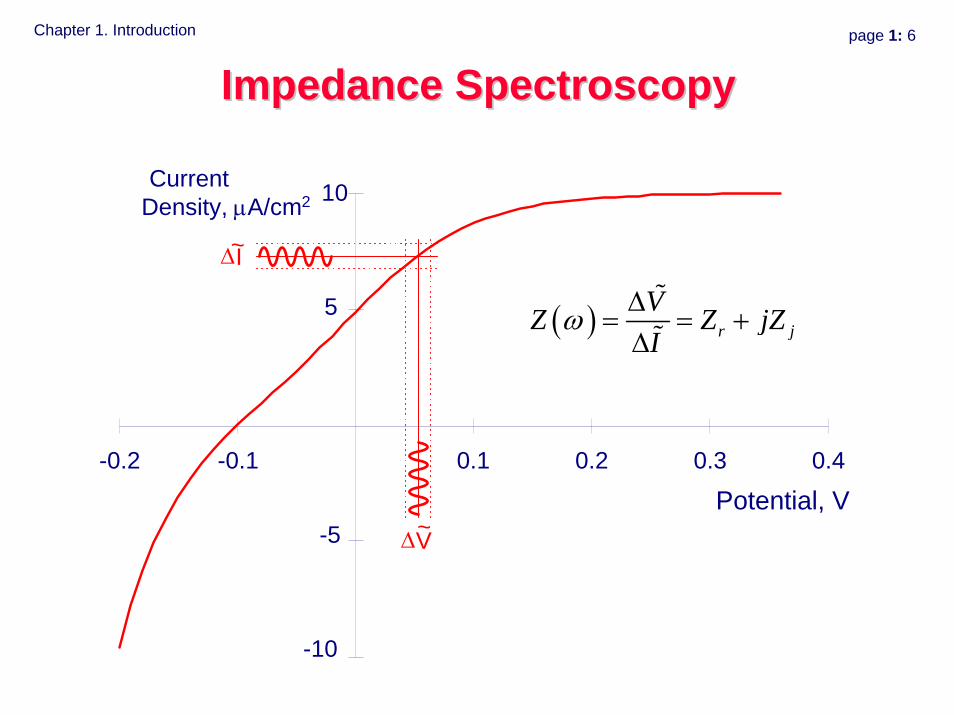
-10
-5
5
10
-0.2 -0.1 0.1 0.2 0.3 0.4
Potential, V
CurrentDensity, μA/cm2
~ΔI
ΔV~
( )
Impedance SpectroscopyImpedance Spectroscopy
r jVZ Z jZI
ω Δ= = +Δ
Chapter 1. Introduction page 1: 7
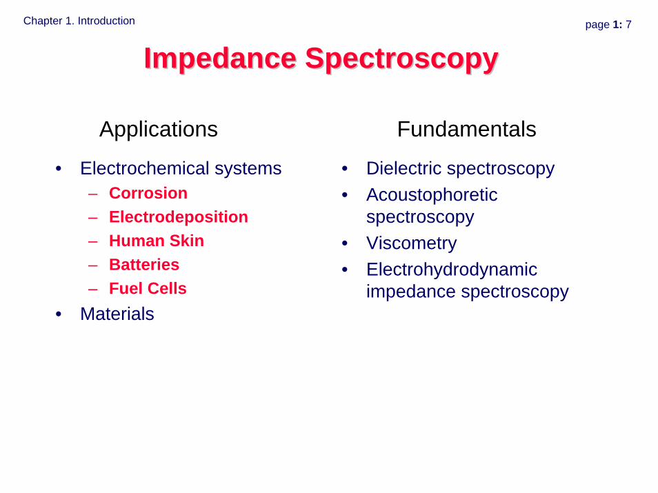
Impedance SpectroscopyImpedance Spectroscopy
• Electrochemical systems– Corrosion– Electrodeposition– Human Skin– Batteries– Fuel Cells
• Materials
• Dielectric spectroscopy• Acoustophoretic
spectroscopy• Viscometry• Electrohydrodynamic
impedance spectroscopy
Applications Fundamentals
Chapter 1. Introduction page 1: 8
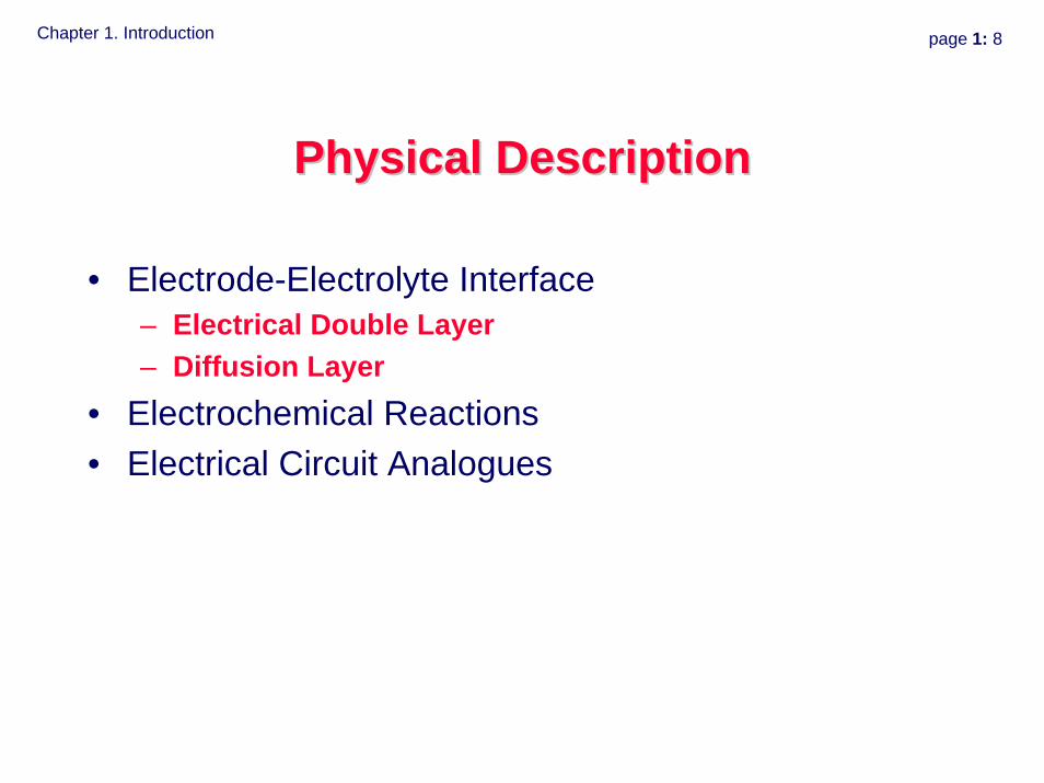
Physical DescriptionPhysical Description
• Electrode-Electrolyte Interface– Electrical Double Layer– Diffusion Layer
• Electrochemical Reactions• Electrical Circuit Analogues
Chapter 1. Introduction page 1: 9
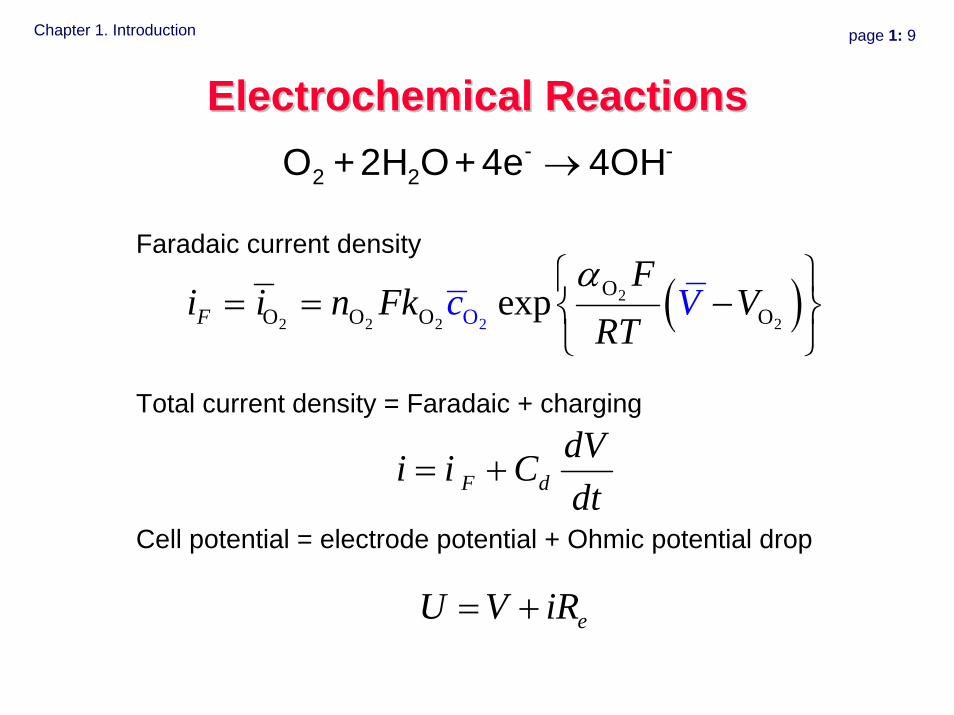
Electrochemical ReactionsElectrochemical Reactions
eU V iR= +
F ddVi i Cdt
= +
( )2 22
2
2 2
OO O O OO expF
Fi i n Fk V
RTc V
α⎧ ⎫= = −⎨ ⎬
⎩ ⎭
Faradaic current density
→- -2 2O +2H O+ 4e 4OH
Total current density = Faradaic + charging
Cell potential = electrode potential + Ohmic potential drop
Chapter 1. Introduction page 1: 10
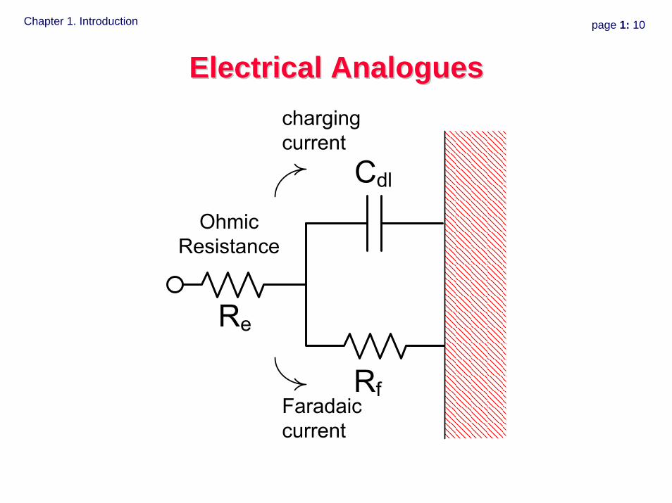
Electrical AnaloguesElectrical Analogues
Chapter 1. Introduction page 1: 11
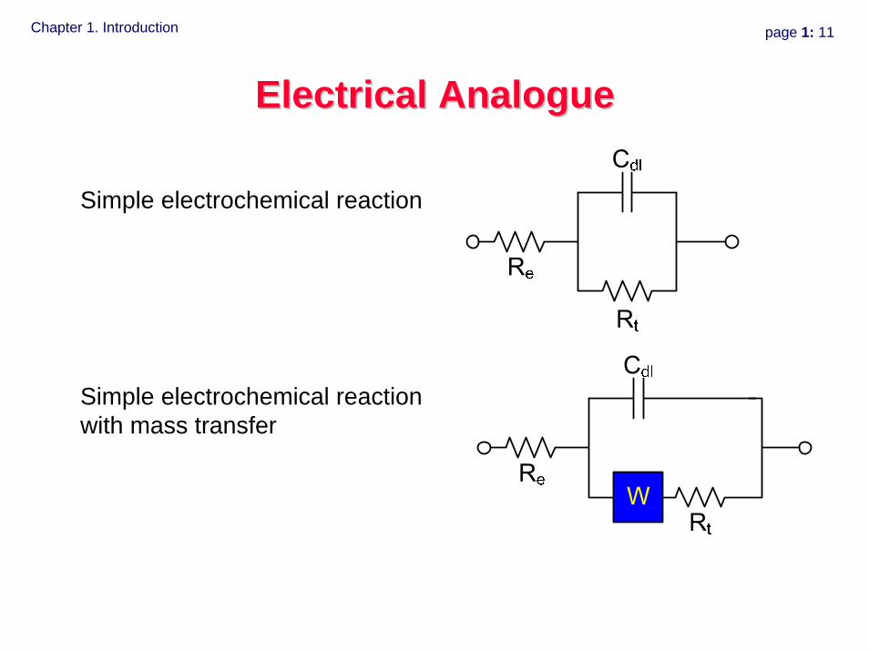
Electrical AnalogueElectrical Analogue
Simple electrochemical reaction
Simple electrochemical reaction with mass transfer
Chapter 1. Introduction page 1: 12
Course ObjectivesCourse Objectives
• Benefits and advantages of impedance spectroscopy• Methods to improve experimental design• Interpretation of data
– graphical representations– regression– error analysis– equivalent circuits– process models
Chapter 1. Introduction page 1: 13
ContentsContents• Chapter 1. Introduction • Chapter 2. Motivation • Chapter 3. Impedance Measurement • Chapter 4. Representations of Impedance Data• Chapter 5. Development of Process Models• Chapter 6. Regression Analysis• Chapter 7. Error Structure• Chapter 8. Kramers-Kronig Relations• Chapter 9. Use of Measurement Models• Chapter 10. Conclusions• Chapter 11. Suggested Reading• Chapter 12. Notation

Chapter 1. Introduction page 1: 14
Chapter 2. Motivation page 2: 1
Electrochemical Impedance Electrochemical Impedance SpectroscopySpectroscopy
Chapter 2. MotivationChapter 2. Motivation
• Comparison of measurements– steady state– step transients– single-sine impedance
• In principle, step and single-sine perturbations yield same results
• Impedance measurements have better error structure
© Mark E. Orazem, 2000-2007. All rights reserved.
Chapter 2. Motivation page 2: 2
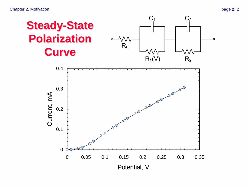
SteadySteady--State State Polarization Polarization
CurveCurve
0
0.1
0.2
0.3
0.4
0 0.05 0.1 0.15 0.2 0.25 0.3 0.35
Potential, V
Cur
rent
, mA
Chapter 2. Motivation page 2: 3
SteadySteady--State TechniquesState Techniques
• Yield information on state after transient is completed• Do not provide information on
– system time constants– capacitance
• Influenced by– Ohmic potential drop– non-stationarity– film growth– coupled reactions
Chapter 2. Motivation page 2: 4
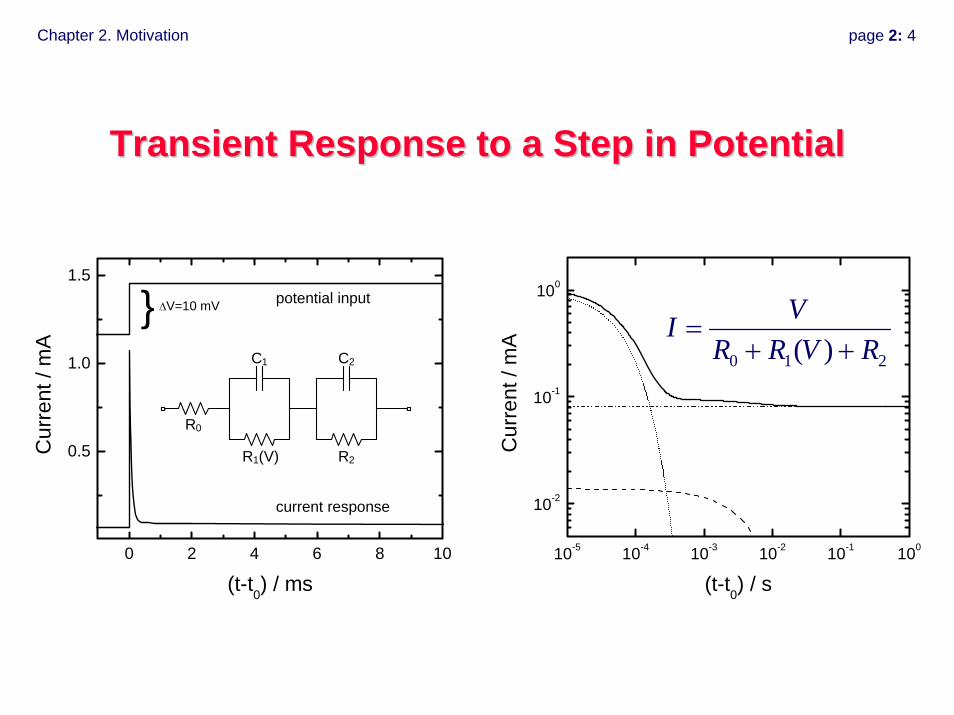
Transient Response to a Step in PotentialTransient Response to a Step in Potential
0 2 4 6 8 10
0.5
1.0
1.5
R0
R1(V)
C1
R2
C2
Cur
rent
/ m
A
(t-t0) / ms
current response
potential inputΔV=10 mV}
10-5 10-4 10-3 10-2 10-1 100
10-2
10-1
100
Cur
rent
/ m
A
(t-t0) / s
210 )( RVRRVI
++=
Chapter 2. Motivation page 2: 5
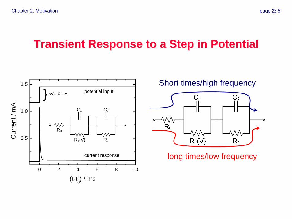
Transient Response to a Step in PotentialTransient Response to a Step in Potential
long times/low frequency
Short times/high frequency
0 2 4 6 8 10
0.5
1.0
1.5
R0
R1(V)
C1
R2
C2
Cur
rent
/ m
A
(t-t0) / ms
current response
potential inputΔV=10 mV}
Chapter 2. Motivation page 2: 6
Transient Techniques: Transient Techniques: potential or current stepspotential or current steps
• Decouples phenomena– characteristic time constants
• mass transfer • kinetics
– capacitance• Limited by accuracy of measurements
– current– potential– time
• Limited by sample rate– <~1 kHz
Chapter 2. Motivation page 2: 7
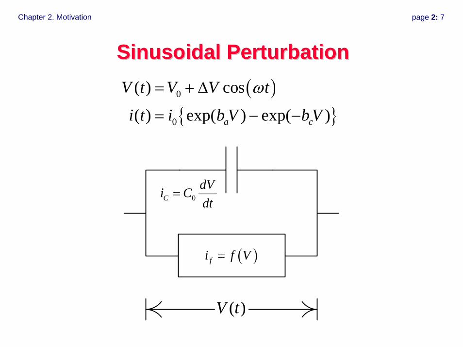
Sinusoidal PerturbationSinusoidal Perturbation
0CdVi Cdt
=
( )fi f V=
( )V t
( ){ }
0
0
( ) cos
( ) exp( ) exp( )a c
V t V V t
i t i b V b V
ω= + Δ
= − −
Chapter 2. Motivation page 2: 8
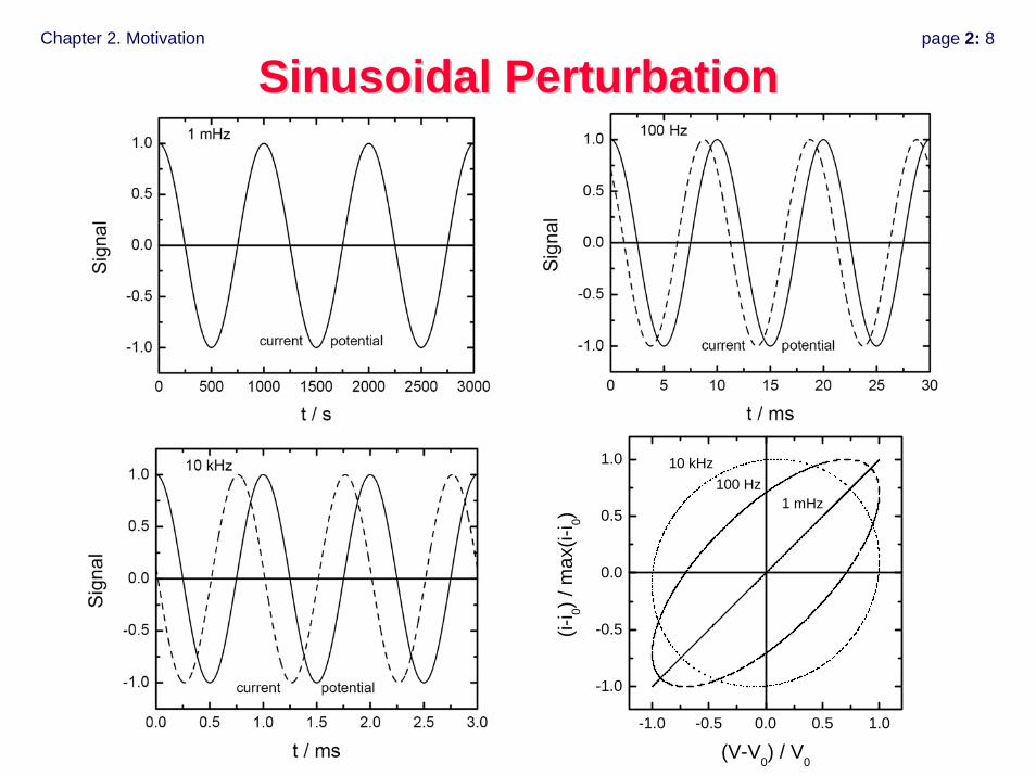
Sinusoidal PerturbationSinusoidal Perturbation
-1.0 -0.5 0.0 0.5 1.0
-1.0
-0.5
0.0
0.5
1.0
1 mHz100 Hz
(i-i 0) /
max
(i-i 0)
(V-V0) / V0
10 kHz

Chapter 2. Motivation page 2: 9
LissajousLissajous RepresentationRepresentation
| |
sin( )
VZI
φ
Δ= =
Δ
= −
OAOB
ODOA
( ) cos( )
( ) cos( )
V t V tVI t tZ
ω
ω φ
= ΔΔ
= +
-1.0 -0.5 0 0.5 1.0
-1.0
-0.5
0
0.5
1.0
Y(t)/
Y 0
X(t)/X0
O D A
B
Chapter 2. Motivation page 2: 10
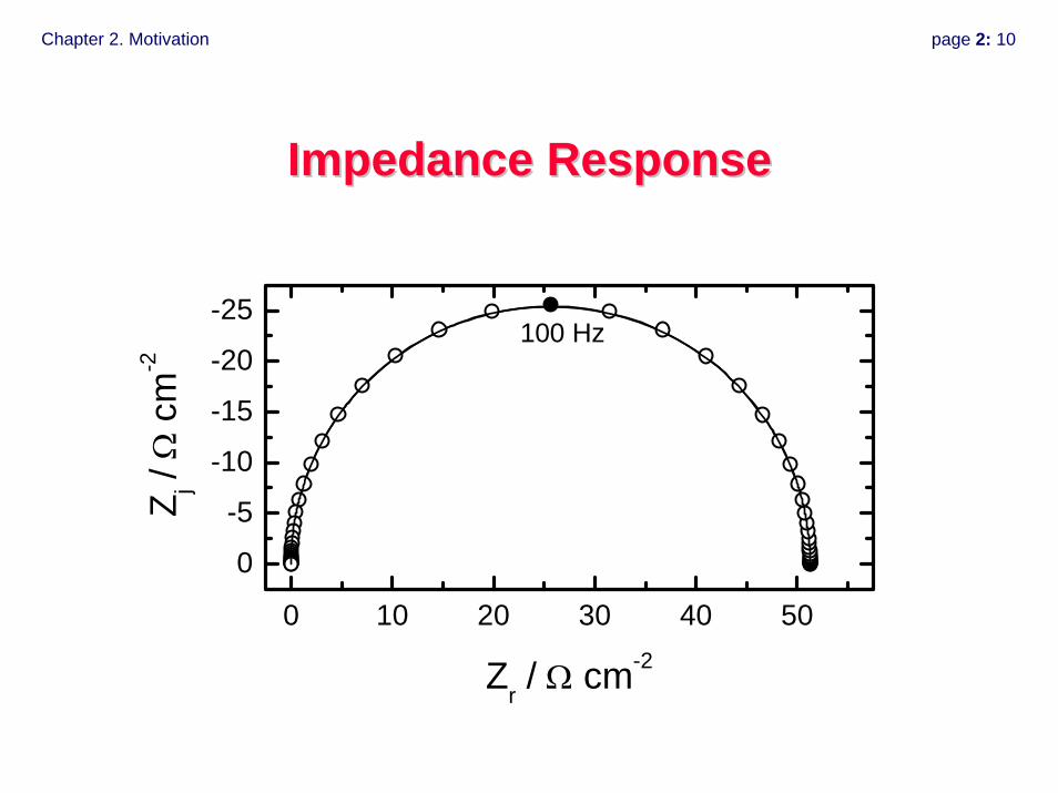
Impedance ResponseImpedance Response
0 10 20 30 40 50
0
-5
-10
-15
-20
-25
Z j / Ω
cm
-2
Zr / Ω cm-2
100 Hz
Chapter 2. Motivation page 2: 11
Impedance SpectroscopyImpedance Spectroscopy• Decouples phenomena
– characteristic time constants• mass transfer • kinetics
– capacitance• Gives same type of information as DC transient.• Improves information content and frequency range by
repeated sampling.• Takes advantage of relationship between real and
imaginary impedance to check consistency.
Chapter 2. Motivation page 2: 12
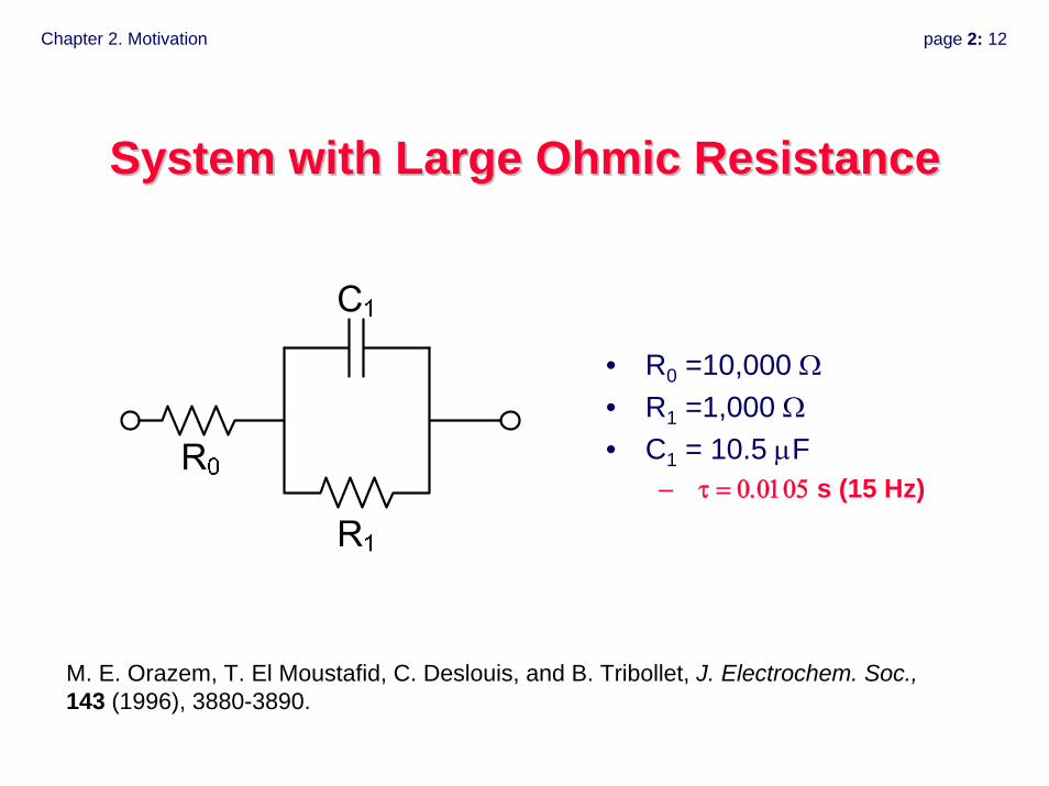
System with Large Ohmic ResistanceSystem with Large Ohmic Resistance
• R0 =10,000 Ω• R1 =1,000 Ω • C1 = 10.5 μF
– τ = 0.0105 s (15 Hz)
M. E. Orazem, T. El Moustafid, C. Deslouis, and B. Tribollet, J. Electrochem. Soc.,143 (1996), 3880-3890.
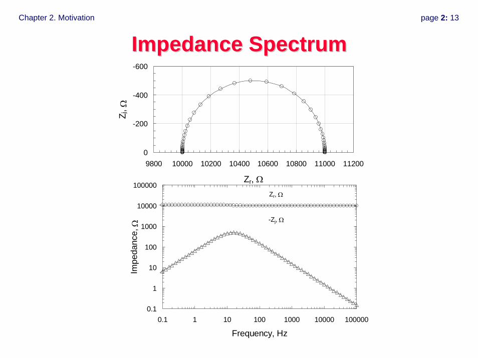
Chapter 2. Motivation page 2: 13
Impedance SpectrumImpedance Spectrum-600
-400
-200
09800 10000 10200 10400 10600 10800 11000 11200
Zr, Ω
Z j, Ω
0.1
1
10
100
1000
10000
100000
0.1 1 10 100 1000 10000 100000
Frequency, Hz
Impe
danc
e, Ω
Zr, Ω
-Zj, Ω
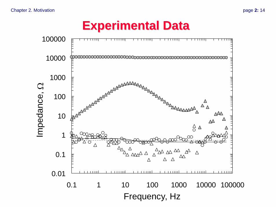
Chapter 2. Motivation page 2: 14
Experimental DataExperimental Data
0.01
0.1
1
10
100
1000
10000
100000
0.1 1 10 100 1000 10000 100000Frequency, Hz
Impe
danc
e, Ω
Chapter 2. Motivation page 2: 15
Impedance Spectroscopy Impedance Spectroscopy vs. Stepvs. Step--Change TransientsChange Transients
• Information sought is the same• Increased sensitivity
– stochastic errors– frequency range– consistency check
• Better decoupling of physical phenomena

Chapter 2. Motivation page 2: 16
Chapter 3. Impedance Measurement page 3: 1
Electrochemical Impedance Electrochemical Impedance SpectroscopySpectroscopy
Chapter 3. Impedance MeasurementChapter 3. Impedance Measurement
• Overview of techniques– A.C. bridge– Lissajous analysis– phase-sensitive detection (lock-in amplifier)– Fourier analysis
• Experimental design
© Mark E. Orazem, 2000-2008. All rights reserved.
Chapter 3. Impedance Measurement page 3: 2
Measurement TechniquesMeasurement Techniques
• A.C. Bridge• Lissajous analysis• Phase-sensitive detection (lock-in amplifier)• Fourier analysis
– digital transfer function analyzer– fast Fourier transform
D. Macdonald, Transient Techniques in Electrochemistry, Plenum Press, NY, 1977.J. Ross Macdonald, editor, Impedance Spectroscopy Emphasizing Solid Materials and Analysis, John Wiley and Sons, New York, 1987.C. Gabrielli, Use and Applications of Electrochemical Impedance Techniques, Technical Report, Schlumberger, Farnborough, England, 1990.
Chapter 3. Impedance Measurement page 3: 3
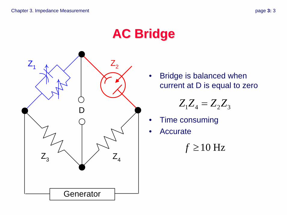
AC BridgeAC Bridge
Generator
Z2Z1
Z3 Z4
D
• Bridge is balanced when current at D is equal to zero
• Time consuming• Accurate
1 4 2 3Z Z Z Z=
10 Hzf ≥
Chapter 3. Impedance Measurement page 3: 4
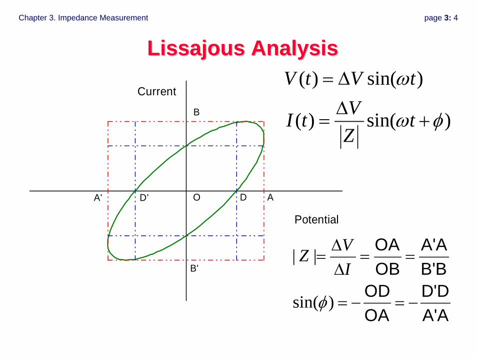
| |
sin( )
VZI
φ
Δ= = =Δ
= − = −
OA A'AOB B'B
OD D'DOA A'A
( ) sin( )
( ) sin( )
V t V tVI t tZ
ω
ω φ
= ΔΔ
= +
Potential
Current
ADO
B
B'
D'A'
LissajousLissajous AnalysisAnalysis
Chapter 3. Impedance Measurement page 3: 5
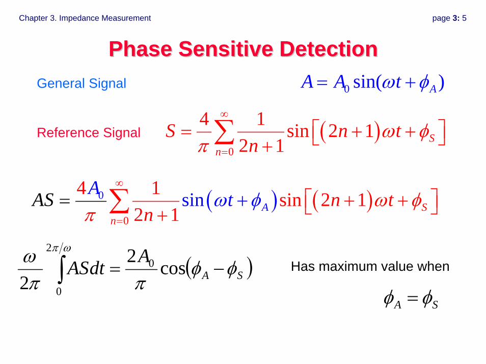
Phase Sensitive DetectionPhase Sensitive Detection0 sin( )AA A tω φ= +
( )0
4 1 sin 2 12 1 S
n
S n tn
ω φπ
∞
=
= + +⎡ ⎤⎣ ⎦+∑
( ) ( )0
0
4 1 si sin 2 12 1
n Sn
A n tn
A A tS ω ω φπ
φ∞
=
+ + ⎦++= ⎡ ⎤⎣∑
General Signal
Reference Signal
( )SAAdtAS φφππ
ω ωπ
−=∫ cos22
02
0
Has maximum value when
A Sφ φ=
Chapter 3. Impedance Measurement page 3: 6
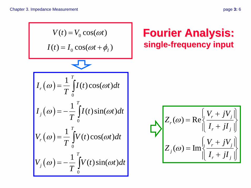
Fourier Analysis:Fourier Analysis:singlesingle--frequency inputfrequency input
0( ) cos( )II t I tω φ= +
0( ) cos( )V t V tω=
( )
( )
( )
( )
0
0
0
0
1 ( ) cos( )
1 ( )sin( )
1 ( )cos( )
1 ( )sin( )
T
r
T
j
T
r
T
j
I I t t dtT
I I t t dtT
V V t t dtT
V V t t dtT
ω ω
ω ω
ω ω
ω ω
=
= −
=
= −
∫
∫
∫
∫
( ) Re
( ) Im
r jr
r j
r jj
r j
V jVZ
I jI
V jVZ
I jI
ω
ω
⎧ ⎫+⎪ ⎪= ⎨ ⎬+⎪ ⎪⎩ ⎭⎧ ⎫+⎪ ⎪= ⎨ ⎬+⎪ ⎪⎩ ⎭
Chapter 3. Impedance Measurement page 3: 7
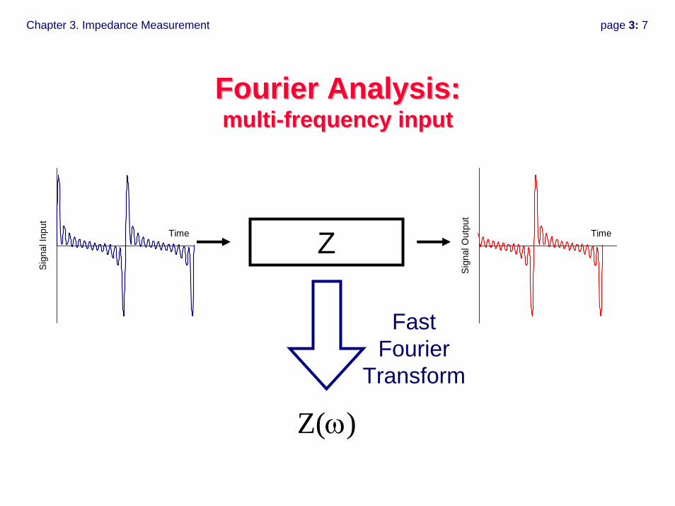
Fourier Analysis:Fourier Analysis:multimulti--frequency inputfrequency input
Time
Sign
al O
utpu
t
Time
Sign
al In
put
Z
Z(ω)
Fast Fourier
Transform
Chapter 3. Impedance Measurement page 3: 8
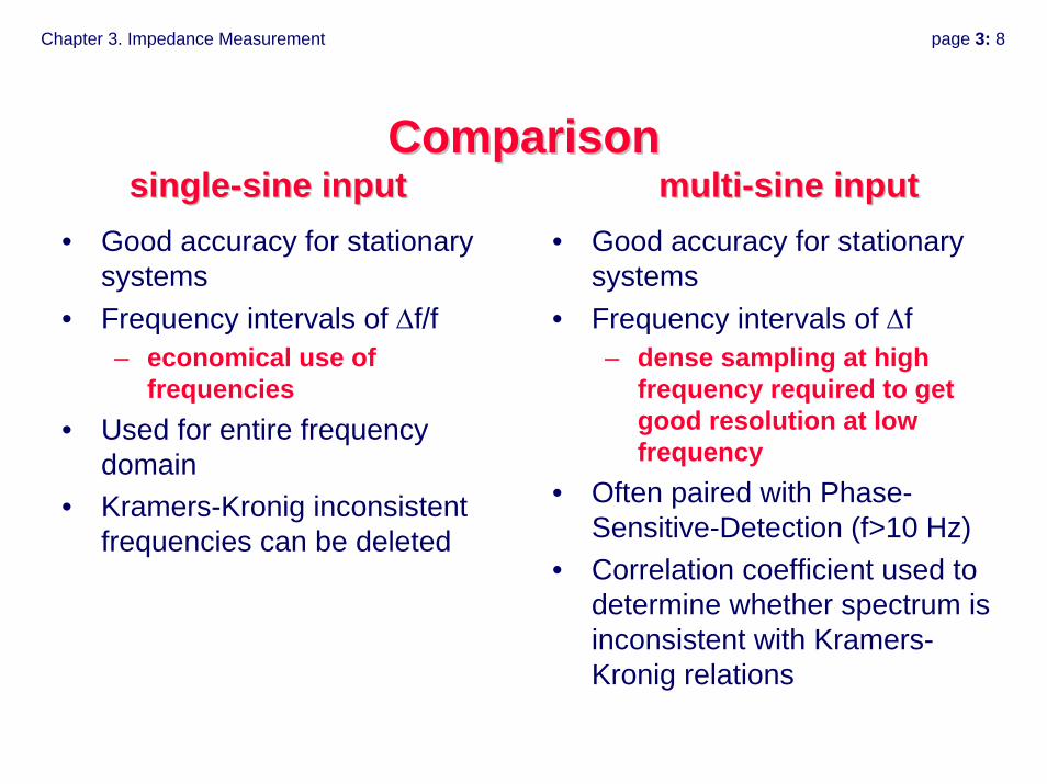
ComparisonComparisonsinglesingle--sine input multisine input multi--sine inputsine input
• Good accuracy for stationary systems
• Frequency intervals of Δf/f– economical use of
frequencies• Used for entire frequency
domain• Kramers-Kronig inconsistent
frequencies can be deleted
• Good accuracy for stationary systems
• Frequency intervals of Δf– dense sampling at high
frequency required to get good resolution at low frequency
• Often paired with Phase-Sensitive-Detection (f>10 Hz)
• Correlation coefficient used to determine whether spectrum is inconsistent with Kramers-Kronig relations
Chapter 3. Impedance Measurement page 3: 9
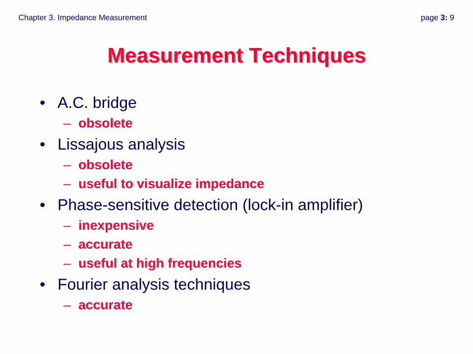
Measurement TechniquesMeasurement Techniques
• A.C. bridge– obsolete
• Lissajous analysis– obsolete– useful to visualize impedance
• Phase-sensitive detection (lock-in amplifier)– inexpensive– accurate– useful at high frequencies
• Fourier analysis techniques– accurate
Chapter 3. Impedance Measurement page 3: 10
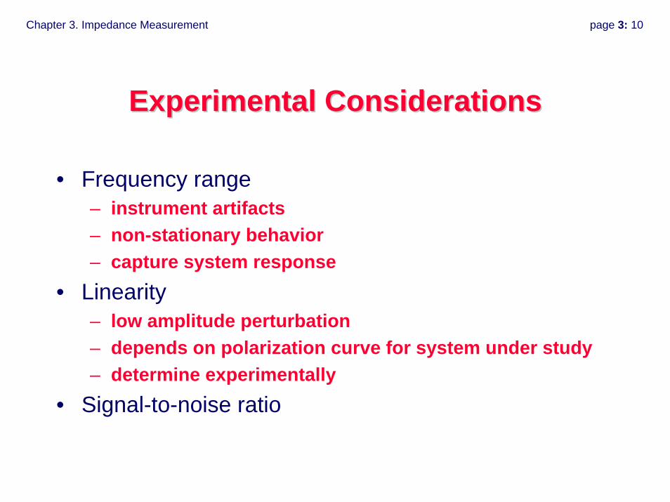
Experimental ConsiderationsExperimental Considerations
• Frequency range– instrument artifacts– non-stationary behavior– capture system response
• Linearity– low amplitude perturbation– depends on polarization curve for system under study– determine experimentally
• Signal-to-noise ratio
Chapter 3. Impedance Measurement page 3: 11
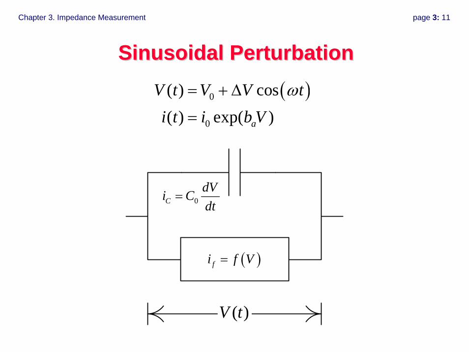
Sinusoidal PerturbationSinusoidal Perturbation
0CdVi Cdt
=
( )fi f V=
( )V t
( )0
0
( ) cos( ) exp( )a
V t V V ti t i b V
ω= + Δ
=

Chapter 3. Impedance Measurement page 3: 12
LinearityLinearity
-1.0 -0.5 0.0 0.5 1.0
-1.0
-0.5
0.0
0.5
1.0 f = 1 mHz 1 mV 20 mV 40 mV
(I-I 0)/m
ax(I-
I 0)
(V-V0)/ΔV-1.0 -0.5 0.0 0.5 1.0
-1.0
-0.5
0.0
0.5
1.0 f = 10 Hz 1 mV 20 mV 40 mV
(I-I 0)/m
ax(I-
I 0)
(V-V0)/ΔV
-1.0 -0.5 0.0 0.5 1.0
-1.0
-0.5
0.0
0.5
1.0 f = 100 Hz 1 mV 20 mV 40 mV
(I-I 0)/m
ax(I-
I 0)
(V-V0)/ΔV-1.0 -0.5 0.0 0.5 1.0
-1.0
-0.5
0.0
0.5
1.0
f = 10 kHz 1 mV 20 mV 40 mV
(I-I 0)
/max
(I-I 0)
(V-V0)/ΔV
Chapter 3. Impedance Measurement page 3: 13
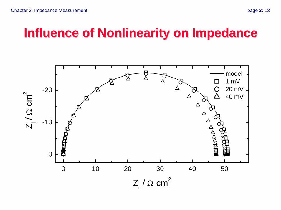
0 10 20 30 40 50
0
-10
-20
model 1 mV 20 mV 40 mV
Z j / Ω
cm
2
Zr / Ω cm2
Influence of Nonlinearity on ImpedanceInfluence of Nonlinearity on Impedance
Chapter 3. Impedance Measurement page 3: 14
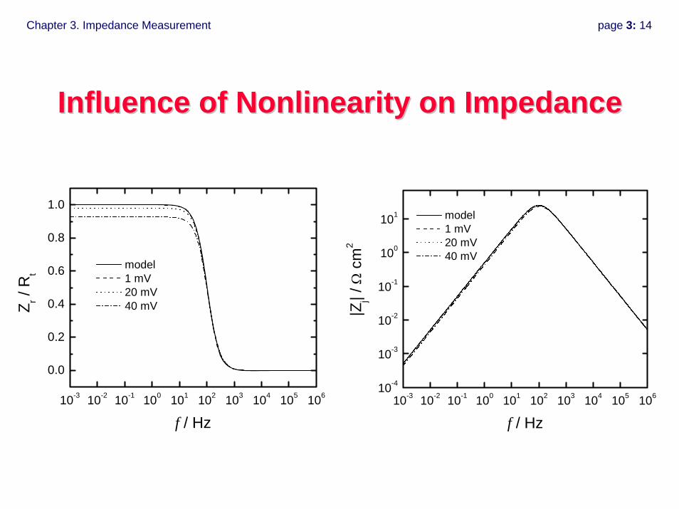
Influence of Nonlinearity on ImpedanceInfluence of Nonlinearity on Impedance
10-3 10-2 10-1 100 101 102 103 104 105 106
0.0
0.2
0.4
0.6
0.8
1.0
model 1 mV 20 mV 40 mVZ r /
Rt
f / Hz10-3 10-2 10-1 100 101 102 103 104 105 106
10-4
10-3
10-2
10-1
100
101 model 1 mV 20 mV 40 mV
|Zj| /
Ω c
m2
f / Hz
Chapter 3. Impedance Measurement page 3: 15
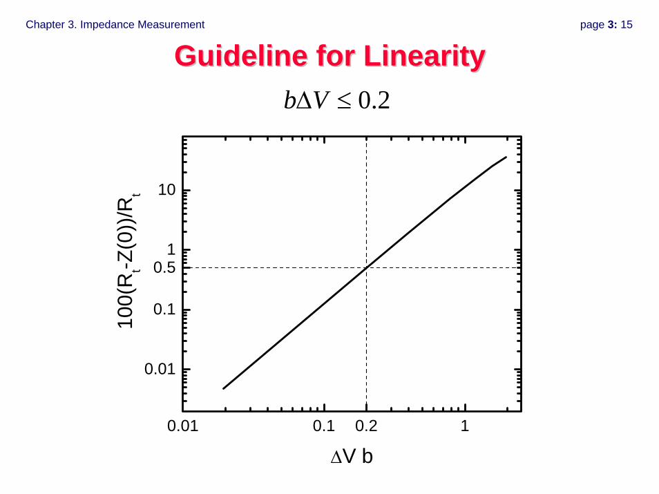
0.01 0.1 0.2 1
0.01
0.1
0.51
10
10
0(R
t-Z(0
))/R
t
ΔV b
Guideline for LinearityGuideline for Linearity0.2b VΔ ≤
Chapter 3. Impedance Measurement page 3: 16
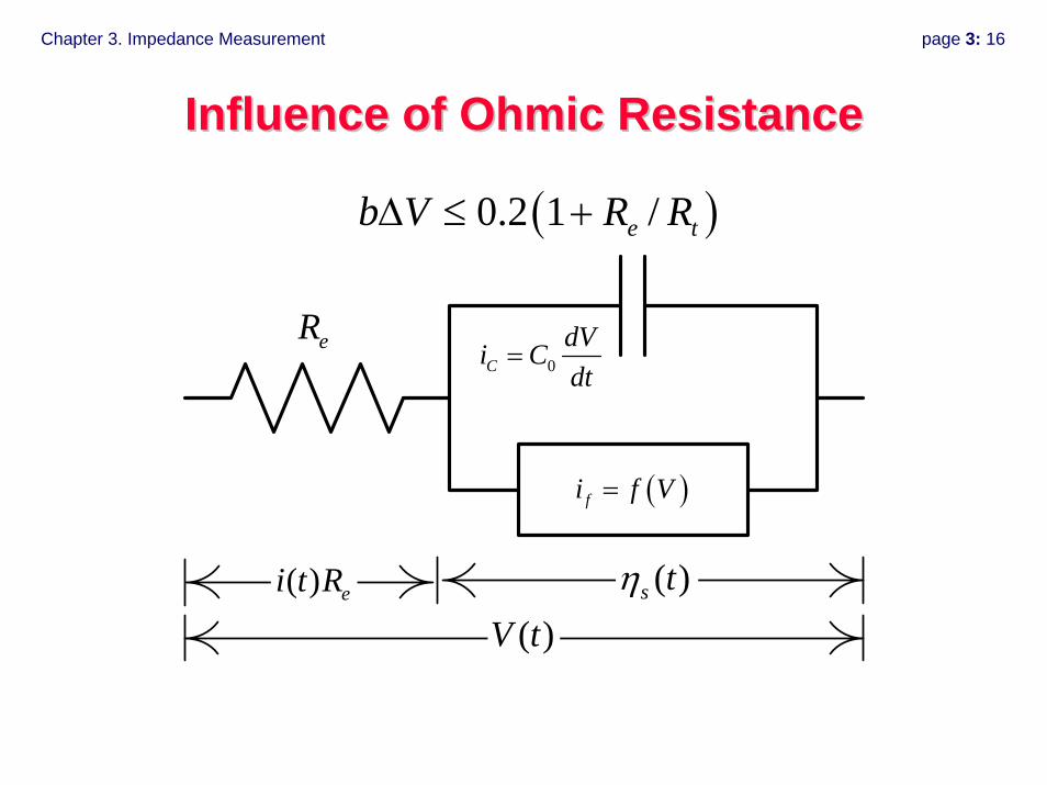
Influence of Ohmic ResistanceInfluence of Ohmic Resistance
0CdVi Cdt
=
( )fi f V=
( )V t( )s tη
eR
( ) ei t R
( )0.2 1 /e tb V R RΔ ≤ +
Chapter 3. Impedance Measurement page 3: 17
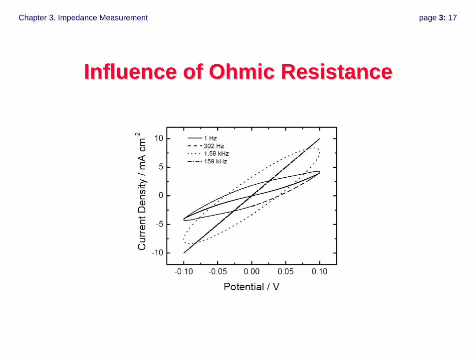
Influence of Ohmic ResistanceInfluence of Ohmic Resistance
Chapter 3. Impedance Measurement page 3: 18
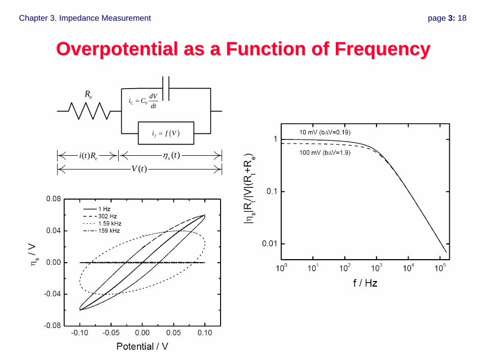
Overpotential as a Function of FrequencyOverpotential as a Function of Frequency
0CdVi Cdt
=
( )fi f V=
( )V t( )s tη
eR
( ) ei t R
Chapter 3. Impedance Measurement page 3: 19
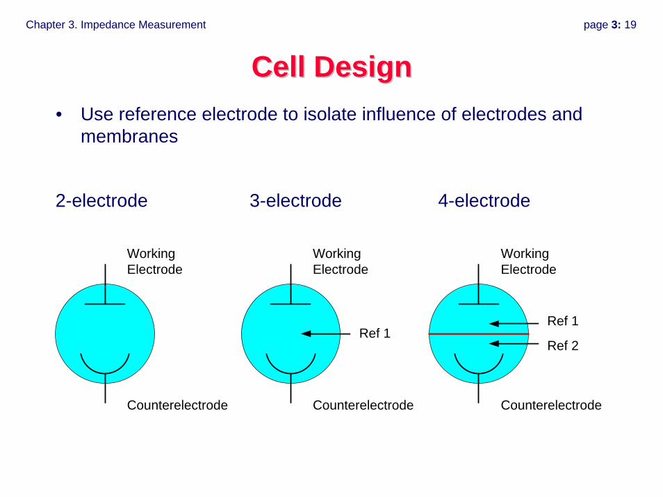
Cell DesignCell Design• Use reference electrode to isolate influence of electrodes and
membranes
WorkingElectrode
Counterelectrode
2-electrode
Ref 1
WorkingElectrode
Counterelectrode
3-electrode
Ref 1
Ref 2
WorkingElectrode
Counterelectrode
4-electrode
Chapter 3. Impedance Measurement page 3: 20
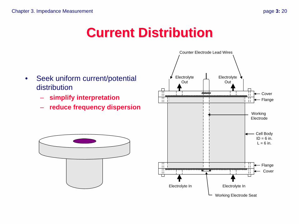
Current DistributionCurrent Distribution
• Seek uniform current/potential distribution
– simplify interpretation– reduce frequency dispersion
Working Electrode Seat
Counter Electrode Lead Wires
Cell BodyID = 6 in.L = 6 in.
Working Electrode
Electrolyte In Electrolyte In
ElectrolyteOut
ElectrolyteOut
FlangeCover
CoverFlange
Chapter 3. Impedance Measurement page 3: 21
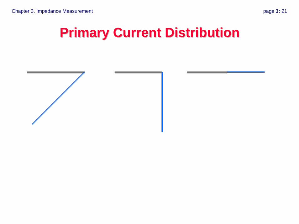
Primary Current DistributionPrimary Current Distribution
Chapter 3. Impedance Measurement page 3: 22
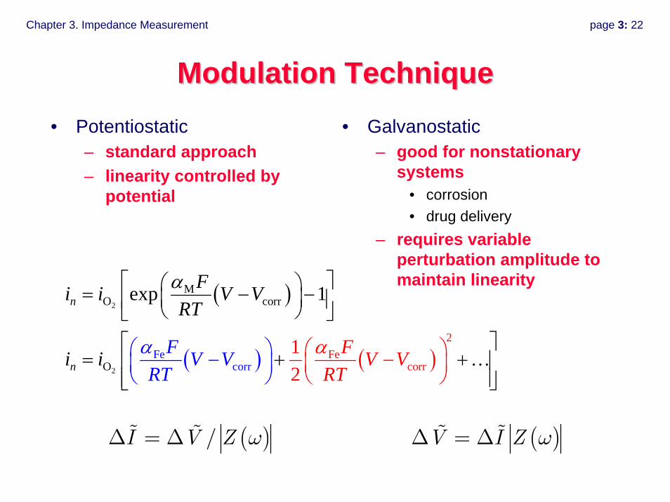
Modulation TechniqueModulation Technique• Potentiostatic
– standard approach– linearity controlled by
potential
• Galvanostatic– good for nonstationary
systems• corrosion• drug delivery
– requires variable perturbation amplitude to maintain linearity
( )
( ) ( )
2
2
MO corr
Fecorr
2Fe
coO rr
exp
12
1n
nF V V
RT
Fi i V
F
V
T
RT
i Vi VR
α
α α
⎡ ⎤⎛ ⎞= − −⎜ ⎟⎢ ⎥⎝ ⎠⎣ ⎦
⎛ ⎞−⎜ ⎟⎝ ⎠
⎡ ⎤= + +⎢ ⎥
⎢ ⎥⎣
⎛ ⎞−⎜⎝ ⎠ ⎦
⎟ …
( ) ( )/I V Z V I Zω ωΔ = Δ Δ = Δ
Chapter 3. Impedance Measurement page 3: 23
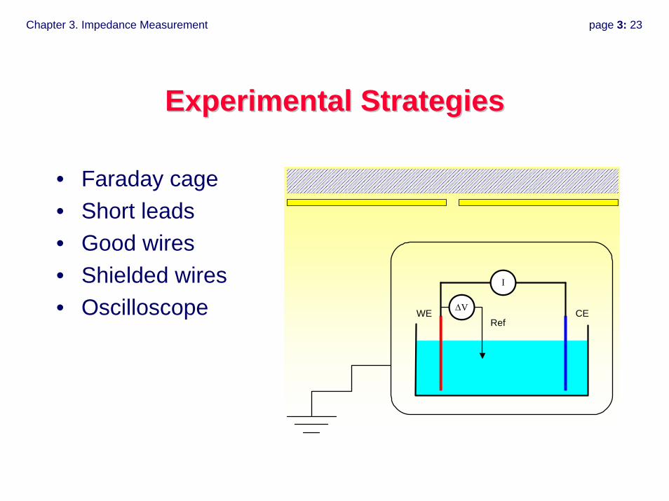
Experimental StrategiesExperimental Strategies
• Faraday cage• Short leads• Good wires• Shielded wires• Oscilloscope
I
ΔVWE CERef
Chapter 3. Impedance Measurement page 3: 24
Reduce Stochastic NoiseReduce Stochastic Noise
• Current measuring range• Integration time/cycles
– long/short integration on some FRAs• Delay time• Avoid line frequency and harmonics (±5 Hz)
– 60 Hz & 120 Hz– 50 Hz & 100 Hz
• Ignore first frequency measured (to avoid start-up transient)
Chapter 3. Impedance Measurement page 3: 25
Reduce NonReduce Non--Stationary EffectsStationary Effects
• Reduce time for measurement– shorter integration (fewer cycles)
• accept more stochastic noise to get less bias error– fewer frequencies
• more measured frequencies yields better parameter estimates• fewer frequencies takes less time
– avoid line frequency and harmonic (±5 Hz)• takes a long time to measure on auto-integration• cannot use data anyway
– select appropriate modulation technique• decide what you want to hold constant (e.g., current or potential)• system drift can increase measurement time on auto-integration
Chapter 3. Impedance Measurement page 3: 26
Reduce Instrument Bias ErrorsReduce Instrument Bias Errors
• Faster potentiostat• Short shielded leads• Faraday cage• Check results
– against electrical circuit– against independently obtained parameters

Chapter 3. Impedance Measurement page 3: 27
Measurement Case StudyMeasurement Case Study
Chapter 3. Impedance Measurement page 3: 28
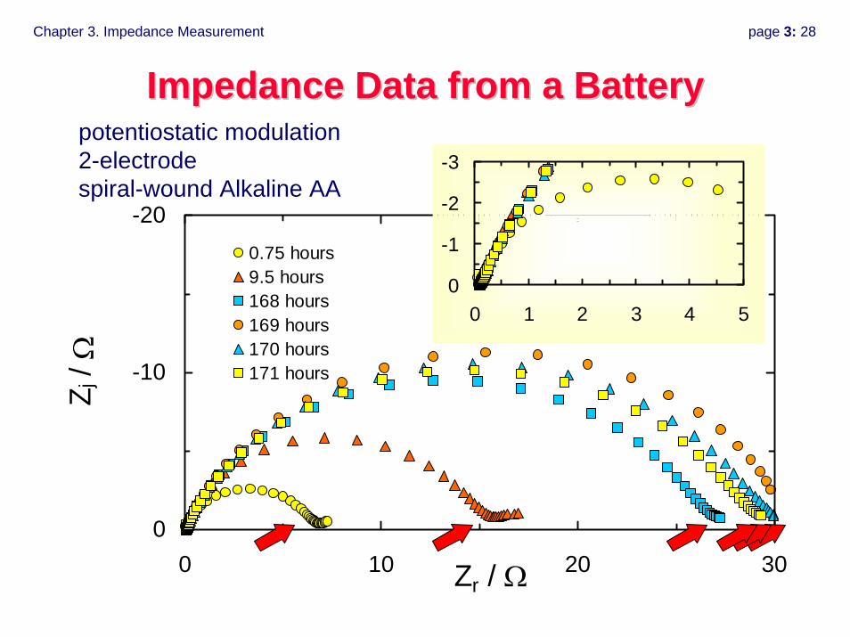
Impedance Data from a BatteryImpedance Data from a Battery
-20
-10
00 10 20 30Zr / Ω
Z j / Ω
0.75 hours9.5 hours168 hours169 hours170 hours171 hours
-3
-2
-1
00 1 2 3 4 5
potentiostatic modulation2-electrodespiral-wound Alkaline AA
Chapter 3. Impedance Measurement page 3: 29
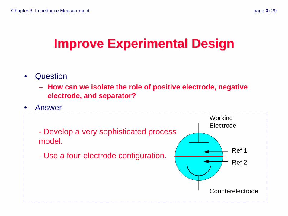
Improve Experimental DesignImprove Experimental Design
• Question– How can we isolate the role of positive electrode, negative
electrode, and separator?• Answer
Ref 1
Ref 2
WorkingElectrode
Counterelectrode
- Develop a very sophisticated process model.
- Use a four-electrode configuration.
Chapter 3. Impedance Measurement page 3: 30
Improve Experimental DesignImprove Experimental Design
• Question– How can we reduce stochastic noise in the measurement?
- Use more cycles during integration. - Add at least a 2-cycle delay.- Ensure use of optimal current measuring resistor.- Check wires and contacts.- Avoid line frequency and harmonics.- Use a Faraday cage.
• Answer
Chapter 3. Impedance Measurement page 3: 31
Improve Experimental DesignImprove Experimental Design
• Question– How can we determine the cause of variability at long times?
- Use the Kramers-Kronig relations to see if data are self-consistent.- Change mode of modulation to variable-amplitude galvanostatic to ensure that the base-line is not changed by the experiment.
• Answer
Chapter 3. Impedance Measurement page 3: 32
Facilitate InterpretationFacilitate Interpretation
• Question– How can we be certain that the instrument is not corrupting
the data?
- Use the Kramers-Kronig relations to see if data are self-consistent.- Build a test circuit with the same impedance response and see if you get the correct result.- Compare results to independently obtained data (such as electrolyte resistance).
• Answer
Chapter 3. Impedance Measurement page 3: 33
Experimental ConsiderationsExperimental Considerations
• Frequency range– instrument artifacts– non-stationary behavior
• Linearity– low amplitude perturbation– depends on polarization curve for system under study– determine experimentally
• Signal-to-noise ratio
Chapter 3. Impedance Measurement page 3: 34
Can We Perform Impedance on Transient Can We Perform Impedance on Transient Systems?Systems?
• Timeframes for measurement– Individual frequency– Individual scan– Multiple scans
Chapter 3. Impedance Measurement page 3: 35
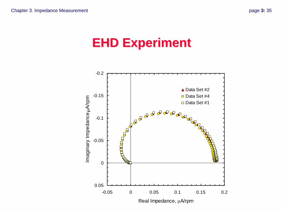
EHD ExperimentEHD Experiment
-0.2
-0.15
-0.1
-0.05
0
0.05-0.05 0 0.05 0.1 0.15 0.2
Real Impedance, μA/rpm
Imag
inar
y Im
peda
nce,
μA/rp
mData Set #2Data Set #4Data Set #1
Chapter 3. Impedance Measurement page 3: 36
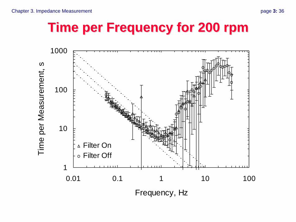
Time per Frequency for 200 rpmTime per Frequency for 200 rpm
1
10
100
1000
0.01 0.1 1 10 100
Frequency, Hz
Tim
e pe
r Mea
sure
men
t, s
1
10
100
10000.01 0.1 1 10 100
Filter OnFilter Off
Chapter 3. Impedance Measurement page 3: 37
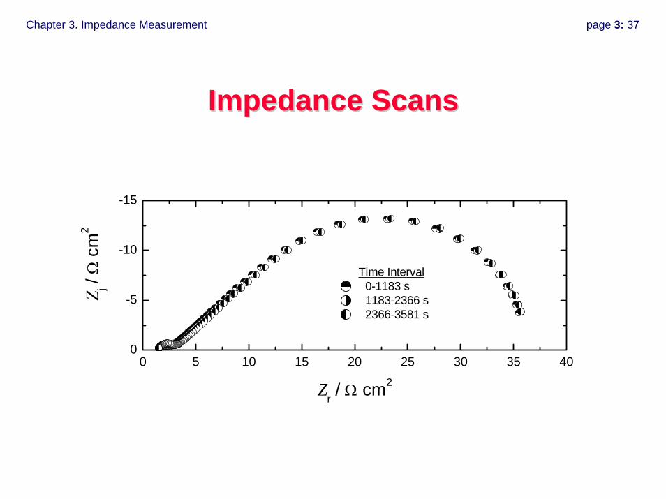
Impedance ScansImpedance Scans
0 5 10 15 20 25 30 35 400
-5
-10
-15
Time Interval 0-1183 s 1183-2366 s 2366-3581 s
Z j / Ω
cm
2
Zr / Ω cm2
Chapter 3. Impedance Measurement page 3: 38
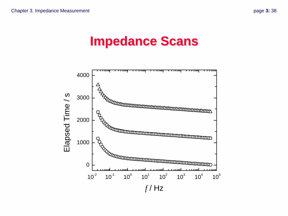
Impedance ScansImpedance Scans
10-2 10-1 100 101 102 103 104 105
0
1000
2000
3000
4000
E
laps
ed T
ime
/ s
f / Hz
Chapter 3. Impedance Measurement page 3: 39
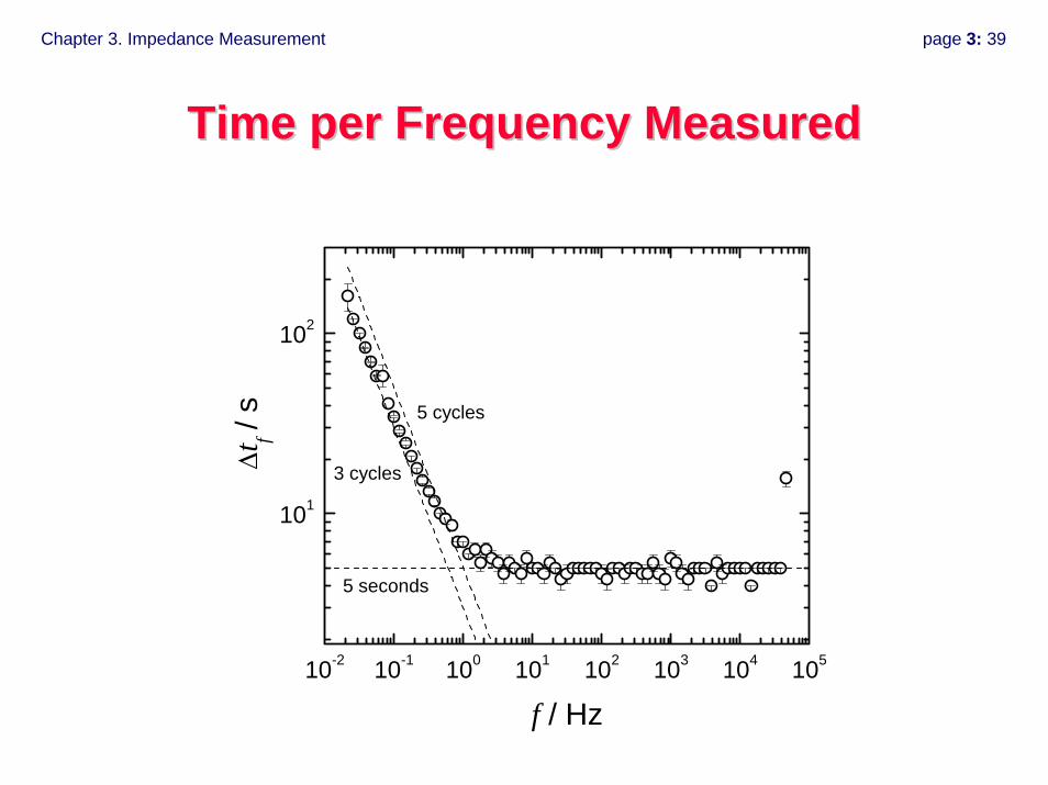
Time per Frequency MeasuredTime per Frequency Measured
10-2 10-1 100 101 102 103 104 105
101
102
Δt f /
s
f / Hz
5 cycles
3 cycles
5 seconds
Chapter 3. Impedance Measurement page 3: 40

Chapter 3. Impedance Measurement page 3: 41

Chapter 4. Representation of Impedance Data page 4: 1
Electrochemical Impedance Electrochemical Impedance SpectroscopySpectroscopy
Chapter 4. Representation of Impedance DataChapter 4. Representation of Impedance Data
• Electrical circuit components• Methods to plot data
– standard plots– subtract electrolyte resistance
• Constant phase elements
© Mark E. Orazem, 2000-2008. All rights reserved.
Chapter 4. Representation of Impedance Data page 4: 2
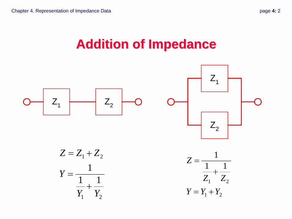
Addition of ImpedanceAddition of Impedance
Z1 Z2
21
21
111
YY
Y
ZZZ
+=
+=
Z1
Z2
21
21
111
YYYZZ
Z
+=
+=
Chapter 4. Representation of Impedance Data page 4: 3
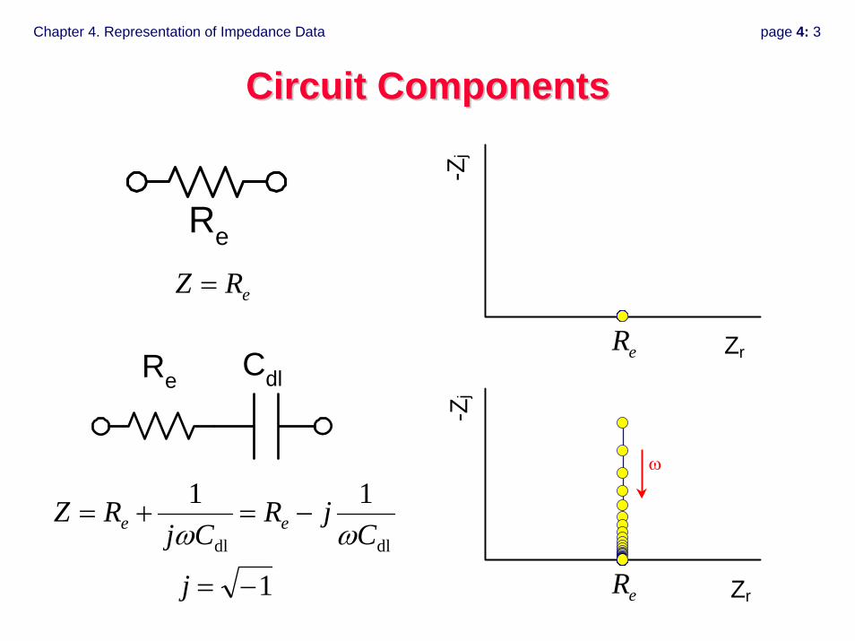
Circuit ComponentsCircuit Components
Re
Zr
-Zj
eRZ =
1
11
dldl
−=
−=+=
j
CjR
CjRZ ee ωω
eR
eR Zr
-Zj
ω
CdlRe
Chapter 4. Representation of Impedance Data page 4: 4
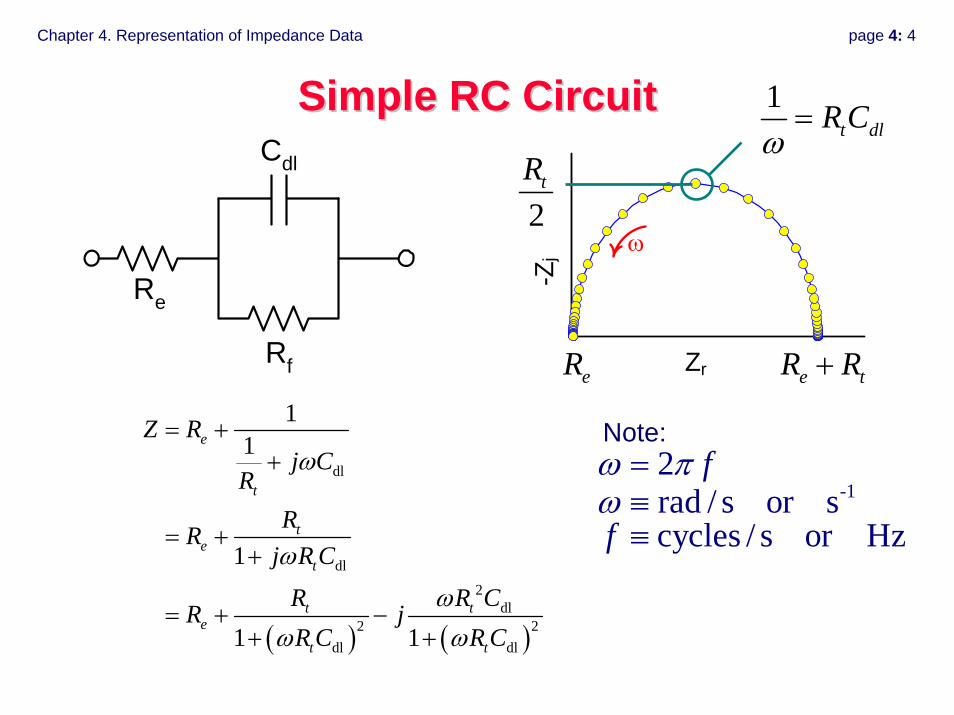
Zr
-Zj ω
Simple RC CircuitSimple RC Circuit
( ) ( )
dl
dl
2dl
2 2dl dl
11
1
1 1
e
t
te
t
t te
t t
Z Rj C
RRR
j R C
R R CR jR C R C
ω
ω
ωω ω
= ++
= ++
= + −+ +
eR e tR R+
2tR
1t dlR C
ω=
Rf
Cdl
Re
-12rad / s or scycles / s or Hz
f
f
ω πω
=≡≡
Note:
Chapter 4. Representation of Impedance Data page 4: 5
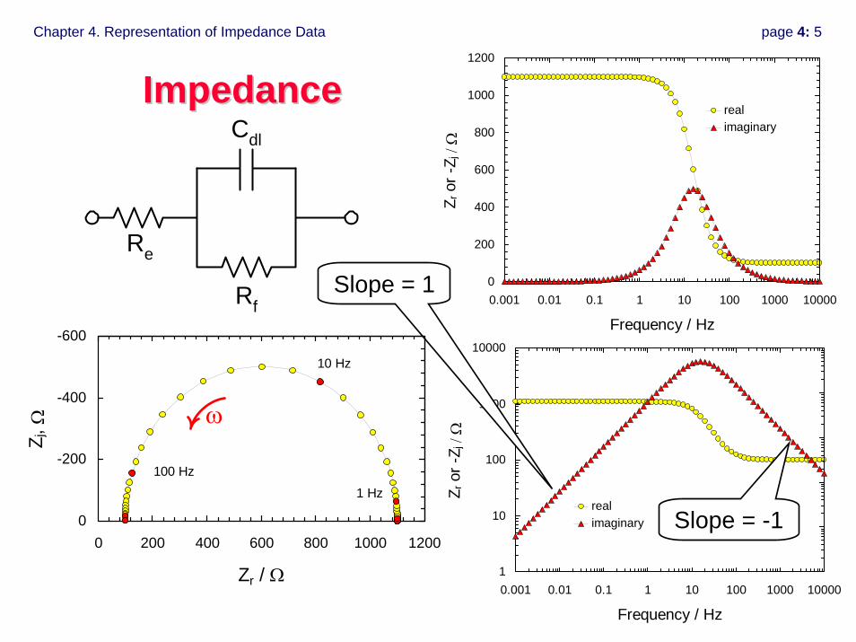
1
10
100
1000
10000
0.001 0.01 0.1 1 10 100 1000 10000
Frequency / Hz
Z r o
r -Z j
/ Ω
realimaginary
ImpedanceImpedance
Slope = 1
Slope = -1
Rf
Cdl
Re
-600
-400
-200
00 200 400 600 800 1000 1200
Zr / Ω
Z j, Ω ω
10 Hz
1 Hz
100 Hz
0
200
400
600
800
1000
1200
0.001 0.01 0.1 1 10 100 1000 10000
Frequency / Hz
Z r o
r -Z j
/ Ω
realimaginary
Chapter 4. Representation of Impedance Data page 4: 6
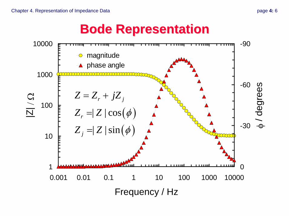
Bode RepresentationBode Representation
1
10
100
1000
10000
0.001 0.01 0.1 1 10 100 1000 10000
Frequency / Hz
|Z| /
Ω-90
-60
-30
0
φ / d
egre
es
magnitudephase angle
( )( )
| | cos
| | sin
r j
r
j
Z Z jZ
Z Z
Z Z
φ
φ
= +
=
=
Chapter 4. Representation of Impedance Data page 4: 7
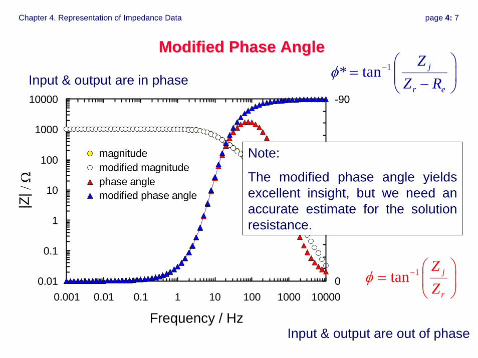
Modified Phase AngleModified Phase Angle
0.01
0.1
1
10
100
1000
10000
0.001 0.01 0.1 1 10 100 1000 10000
Frequency / Hz
|Z| /
Ω
-90
-60
-30
0
φ∗ /
degr
eesmagnitude
modified magnitudephase anglemodified phase angle
1* tan j
r e
ZZ R
φ − ⎛ ⎞= ⎜ ⎟−⎝ ⎠Input & output are in phase
Input & output are out of phase
1tan j
r
ZZ
φ − ⎛ ⎞= ⎜ ⎟
⎝ ⎠
Note:
The modified phase angle yields excellent insight, but we need an accurate estimate for the solution resistance.
Chapter 4. Representation of Impedance Data page 4: 8
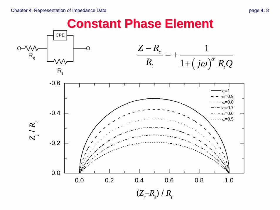
Constant Phase ElementConstant Phase Element
( )1
1e
t t
Z RR j R Qαω−
= ++
Rt
Re
CPE
0.0 0.2 0.4 0.6 0.8 1.00.0
-0.2
-0.4
-0.6 α=1 α=0.9 α=0.8 α=0.7 α=0.6 α=0.5
Z j / R t
(Zr−Re) / Rt
Chapter 4. Representation of Impedance Data page 4: 9
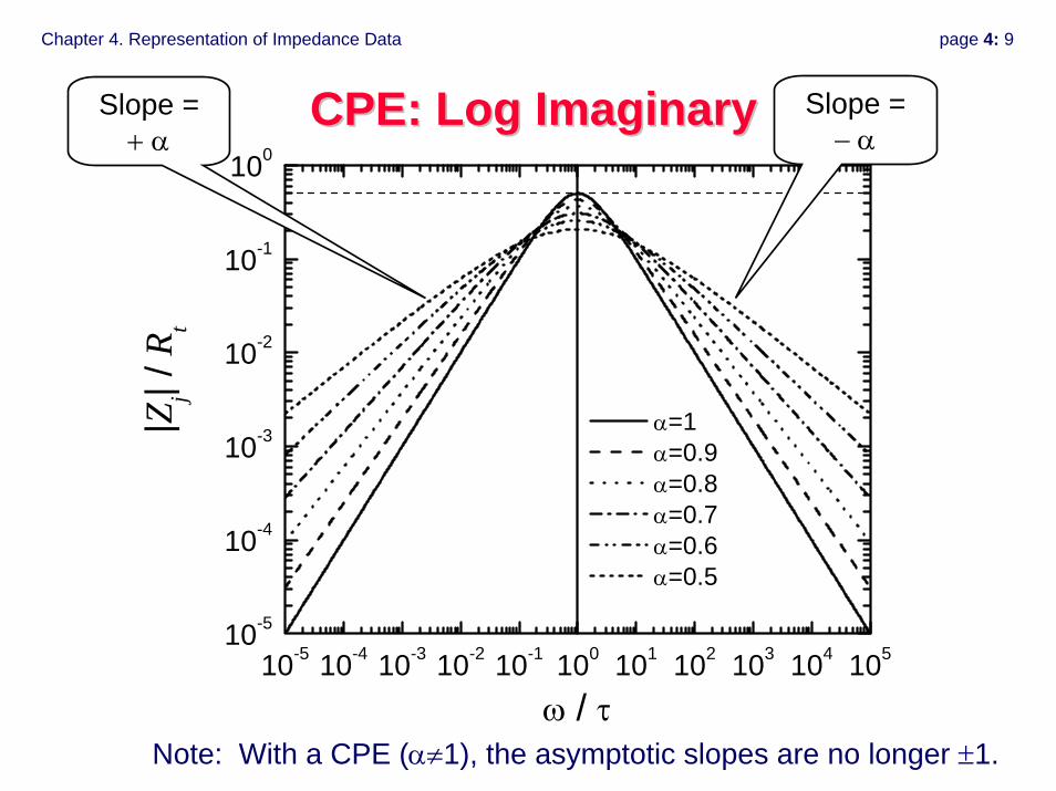
10-5 10-4 10-3 10-2 10-1 100 101 102 103 104 10510-5
10-4
10-3
10-2
10-1
100
α=1 α=0.9 α=0.8 α=0.7 α=0.6 α=0.5
|Zj| /
Rt
ω / τ
CPE: Log ImaginaryCPE: Log Imaginary
Note: With a CPE (α≠1), the asymptotic slopes are no longer ±1.
Slope = − α
Slope = + α
Chapter 4. Representation of Impedance Data page 4: 10
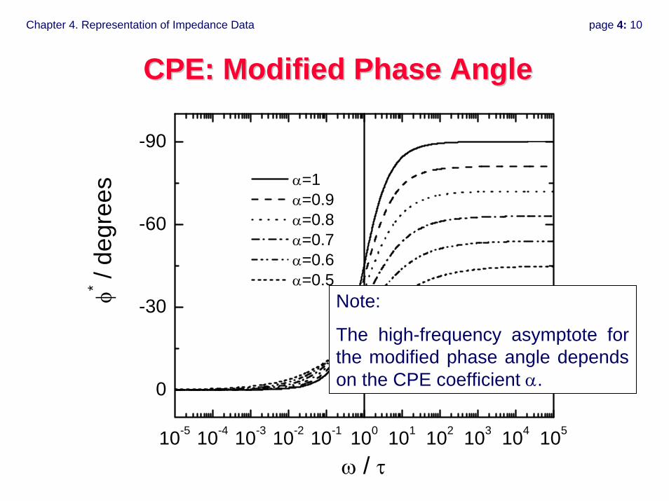
CPE: Modified Phase AngleCPE: Modified Phase Angle
10-5 10-4 10-3 10-2 10-1 100 101 102 103 104 105
0
-30
-60
-90
α=1 α=0.9 α=0.8 α=0.7 α=0.6 α=0.5
φ* / de
gree
s
ω / τ
Note:
The high-frequency asymptote for the modified phase angle depends on the CPE coefficient α.
Chapter 4. Representation of Impedance Data page 4: 11
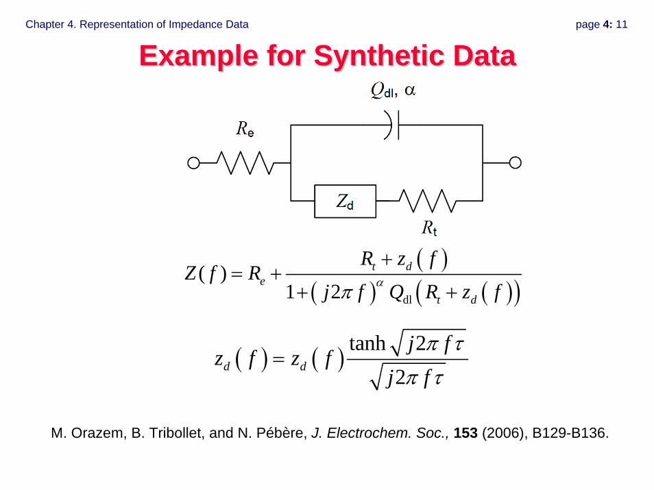
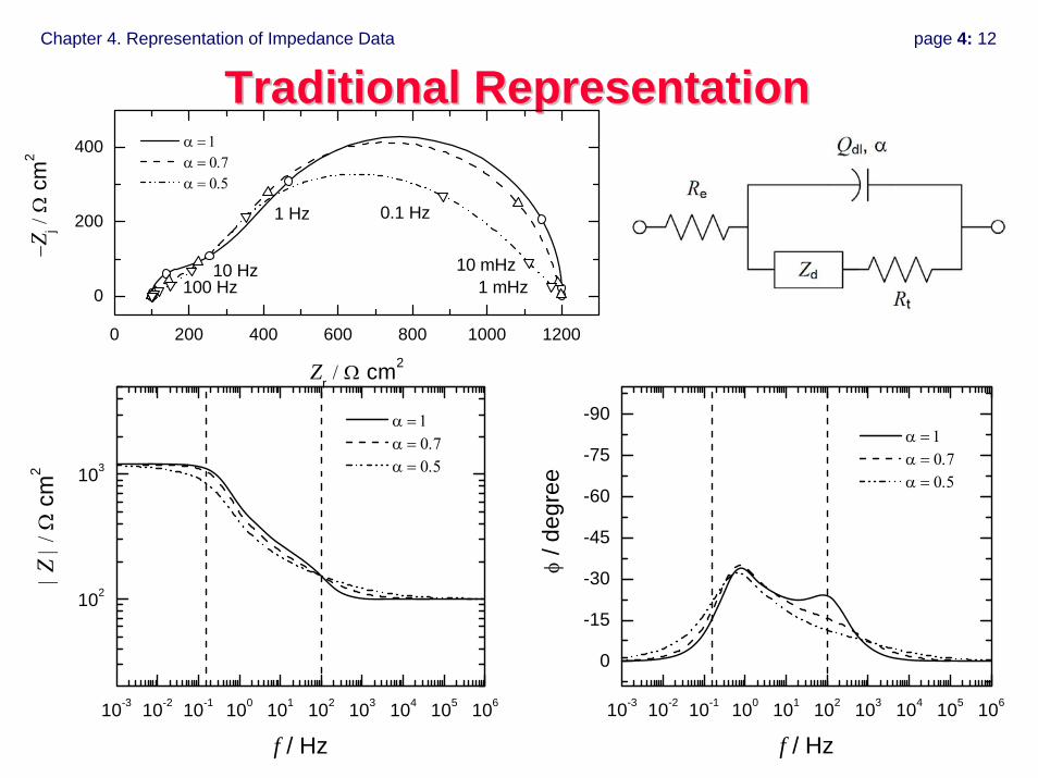
Example for Synthetic DataExample for Synthetic Data
( )( ) ( )( )dl
( )1 2
t de
t d
R z fZ f R
j f Q R z fαπ
+= +
+ +
( ) ( ) tanh 22d d
j fz f z f
j fπ τ
π τ=
M. Orazem, B. Tribollet, and N. Pébère, J. Electrochem. Soc., 153 (2006), B129-B136.
Chapter 4. Representation of Impedance Data page 4: 12
Traditional RepresentationTraditional Representation
0 200 400 600 800 1000 1200
0
200
400 α = 1 α = 0.7 α = 0.5
1 mHz100 Hz10 Hz
1 Hz 0.1 Hz
−Zj /
Ω c
m2
Zr / Ω cm2
10 mHz
10-3 10-2 10-1 100 101 102 103 104 105 106
102
103
α = 1 α = 0.7 α = 0.5
| Z |
/ Ω c
m2
f / Hz10-3 10-2 10-1 100 101 102 103 104 105 106
0
-15
-30
-45
-60
-75
-90 α = 1 α = 0.7 α = 0.5
φ / d
egre
e
f / Hz
Chapter 4. Representation of Impedance Data page 4: 13
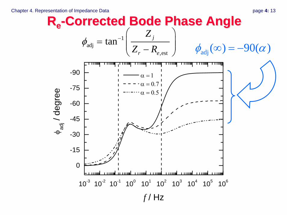
RRee--Corrected Bode Phase AngleCorrected Bode Phase Angle1
adj,est
tan j
r e
ZZ R
φ − ⎛ ⎞= ⎜ ⎟⎜ ⎟−⎝ ⎠ adj ( ) 90( )φ α∞ = −
10-3 10-2 10-1 100 101 102 103 104 105 106
0
-15
-30
-45
-60
-75
-90 α = 1 α = 0.7 α = 0.5
φ ad
j / de
gree
f / Hz
Chapter 4. Representation of Impedance Data page 4: 14
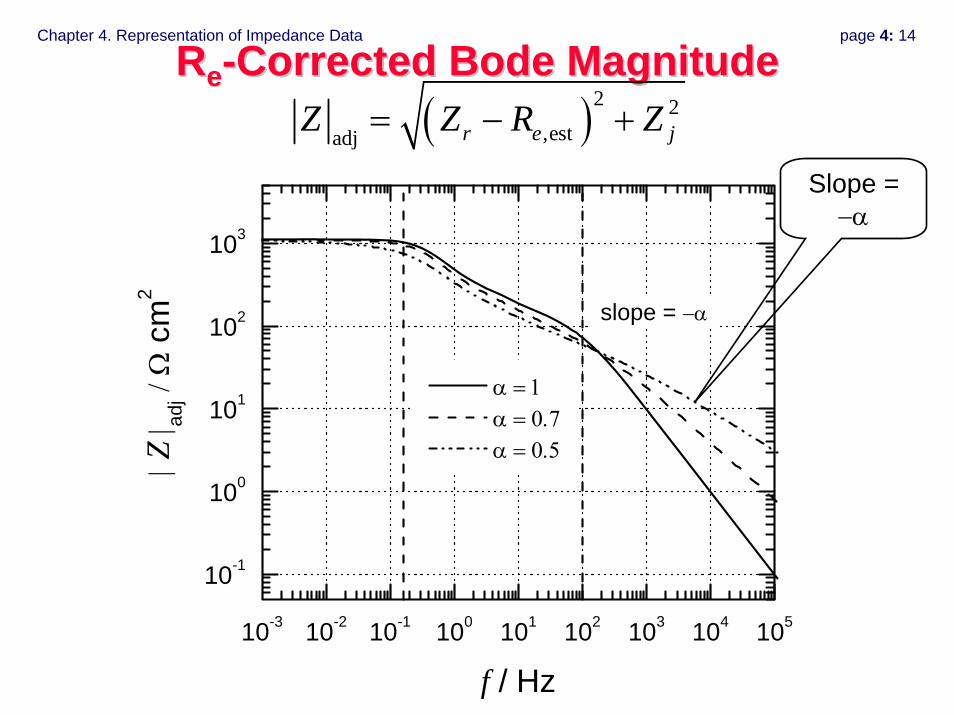
RRee--Corrected Bode MagnitudeCorrected Bode Magnitude( )2 2
,estadj r e jZ Z R Z= − +
Slope = −α
10-3 10-2 10-1 100 101 102 103 104 105
10-1
100
101
102
103
α = 1 α = 0.7 α = 0.5
| Z
| adj /
Ω c
m2
f / Hz
slope = −α
Chapter 4. Representation of Impedance Data page 4: 15
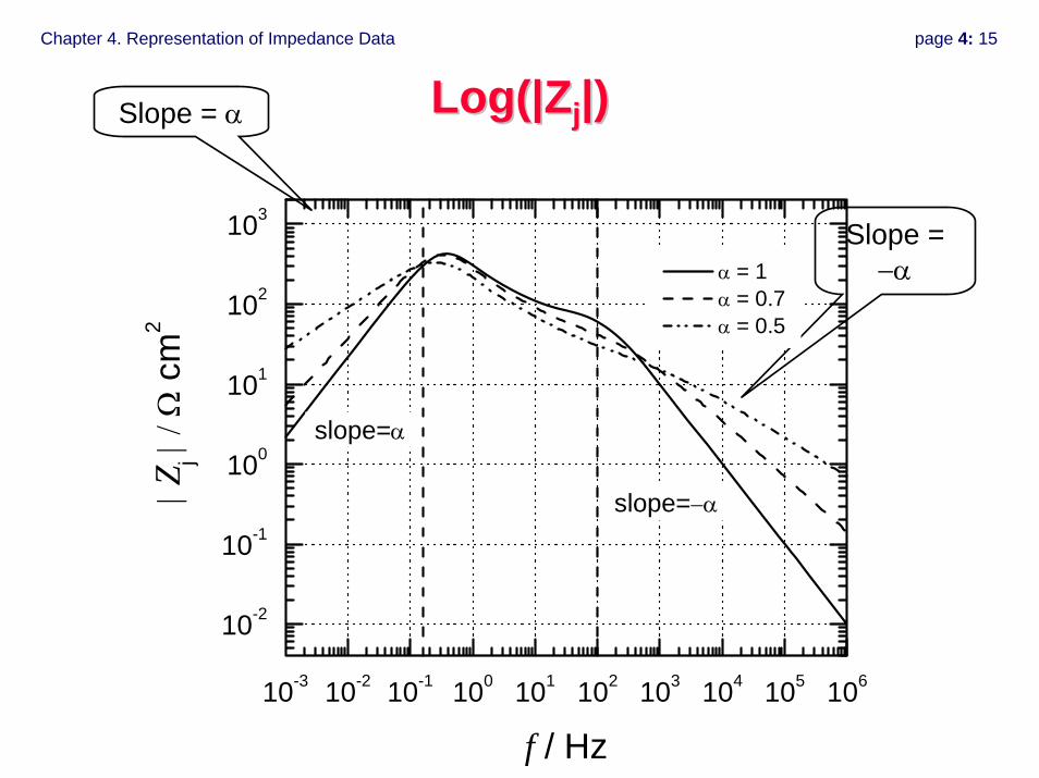
Log(|ZLog(|Zjj|)|)
Slope = −α
Slope = α
10-3 10-2 10-1 100 101 102 103 104 105 106
10-2
10-1
100
101
102
103
α = 1 α = 0.7 α = 0.5
slope=α
slope=−α
| Z
j | / Ω
cm
2
f / Hz
Chapter 4. Representation of Impedance Data page 4: 16
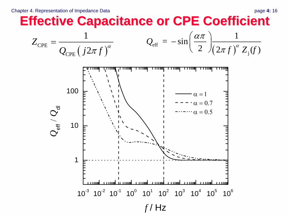
Effective Capacitance or CPE CoefficientEffective Capacitance or CPE Coefficient
( )effj
1 = sin2 2 ( )
Qf Z fα
αππ
⎛ ⎞− ⎜ ⎟⎝ ⎠( )CPE
CPE
12
ZQ j f απ
=
10-3 10-2 10-1 100 101 102 103 104 105 106
1
10
100 α = 1 α = 0.7 α = 0.5
Q
eff /
Qdl
f / Hz
Chapter 4. Representation of Impedance Data page 4: 17
• Re-Corrected Bode Plots (Phase Angle) – Shows expected high-frequency behavior for surface– High-Frequency limit reveals CPE behavior
• Re-Corrected Bode Plots (Magnitude) – High-Frequency slope related to CPE behavior
• Log|Zj|– Slopes related to CPE behavior– Peaks reveal characteristic time constants
• Effective Capacitance– High-Frequency limit yields capacitance or CPE
coefficient
Alternative PlotsAlternative Plots

Chapter 4. Representation of Impedance Data page 4: 18
ApplicationApplication
Chapter 4. Representation of Impedance Data page 4: 19
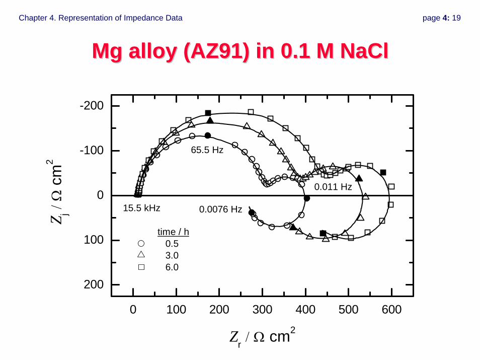
Mg alloy (AZ91) in 0.1 M Mg alloy (AZ91) in 0.1 M NaClNaCl
0 100 200 300 400 500 600
200
100
0
-100
-200
15.5 kHz
0.011 Hz
0.0076 Hz
time / h 0.5 3.0 6.0
Z j / Ω
cm
2
Zr / Ω cm2
65.5 Hz

Chapter 4. Representation of Impedance Data page 4: 20
Proposed ModelProposed Model
22 Mg(OH)OH2Mg
4
4
⎯⎯←⎯→⎯
+−
−+
k
k
OHMgOMg(OH) 25-k
5k
2 +⎯⎯←⎯→⎯
( ) −+ +⎯→⎯ eMgMg ads1k
( ) 2212
2ads HOHMgOHMg 2 ++⎯→⎯+ −++ k
( ) −++ +⎯⎯←⎯→⎯
−
eMgMg 2ads
3
3
k
k
G. Baril, G. Galicia, C. Deslouis, N. Pébère, B. Tribollet, and V. Vivier, J. Electrochem. Soc.,154 (2007), C108-C113
“negative difference effect”(NDE)

Chapter 4. Representation of Impedance Data page 4: 21
0 100 200 300 400 500 600
200
100
0
-100
-200
15.5 kHz
0.011 Hz
0.0076 Hz
time / h 0.5 3.0 6.0
Z j / Ω
cm
2
Zr / Ω cm2
65.5 Hz
Physical InterpretationPhysical Interpretationdiffusion of Mg2+
( ) −+ +⎯→⎯ eMgMg ads1k
( ) −++ +⎯⎯←⎯→⎯
−
eMgMg 2ads
3
3
k
k
relaxation of (Mg+)ads.intermediate
Chapter 4. Representation of Impedance Data page 4: 22
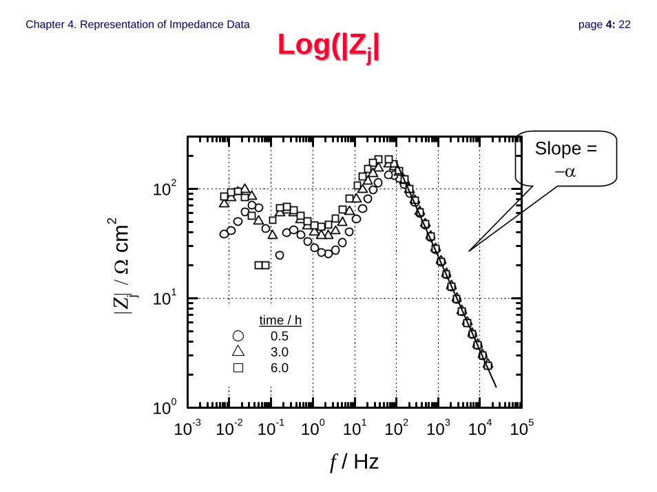
Log(|ZLog(|Zjj||
Slope = −α
10-3 10-2 10-1 100 101 102 103 104 105100
101
102
time / h 0.5 3.0 6.0
|Z
j| / Ω
cm
2
f / Hz
Chapter 4. Representation of Impedance Data page 4: 23
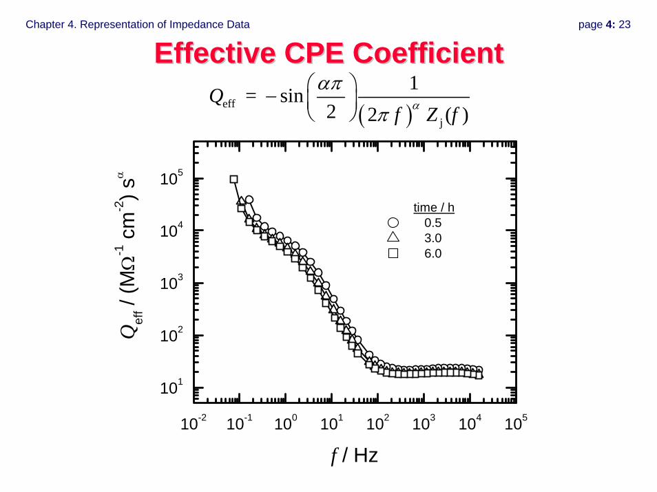
Effective CPE CoefficientEffective CPE Coefficient
( )effj
1 = sin2 2 ( )
Qf Z fα
αππ
⎛ ⎞− ⎜ ⎟⎝ ⎠
10-2 10-1 100 101 102 103 104 105
101
102
103
104
105
time / h 0.5 3.0 6.0
Q
eff /
(MΩ
-1 c
m-2) s
α
f / Hz
Chapter 4. Representation of Impedance Data page 4: 24
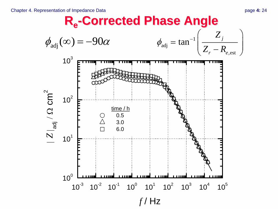
RRee--Corrected Phase AngleCorrected Phase Angle
adj ( ) 90φ α∞ = − 1adj
,est
tan j
r e
ZZ R
φ − ⎛ ⎞= ⎜ ⎟⎜ ⎟−⎝ ⎠
10-3 10-2 10-1 100 101 102 103 104 105100
101
102
103
time / h 0.5 3.0 6.0
| Z
| adj /
Ω c
m2
f / Hz
Chapter 4. Representation of Impedance Data page 4: 25
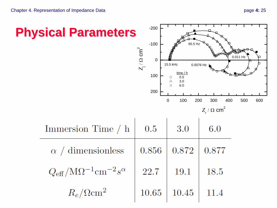
Physical ParametersPhysical Parameters
0 100 200 300 400 500 600
200
100
0
-100
-200
15.5 kHz
0.011 Hz
0.0076 Hz
time / h 0.5 3.0 6.0
Z j / Ω
cm
2
Zr / Ω cm2
65.5 Hz

Chapter 4. Representation of Impedance Data page 4: 26
Experimental device for LEISExperimental device for LEIS
appliedlocal
local
VZ
iΔ
=Δ
layer
Chapter 4. Representation of Impedance Data page 4: 27
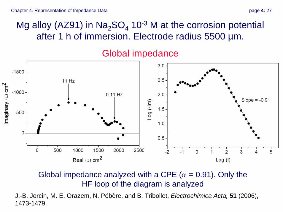
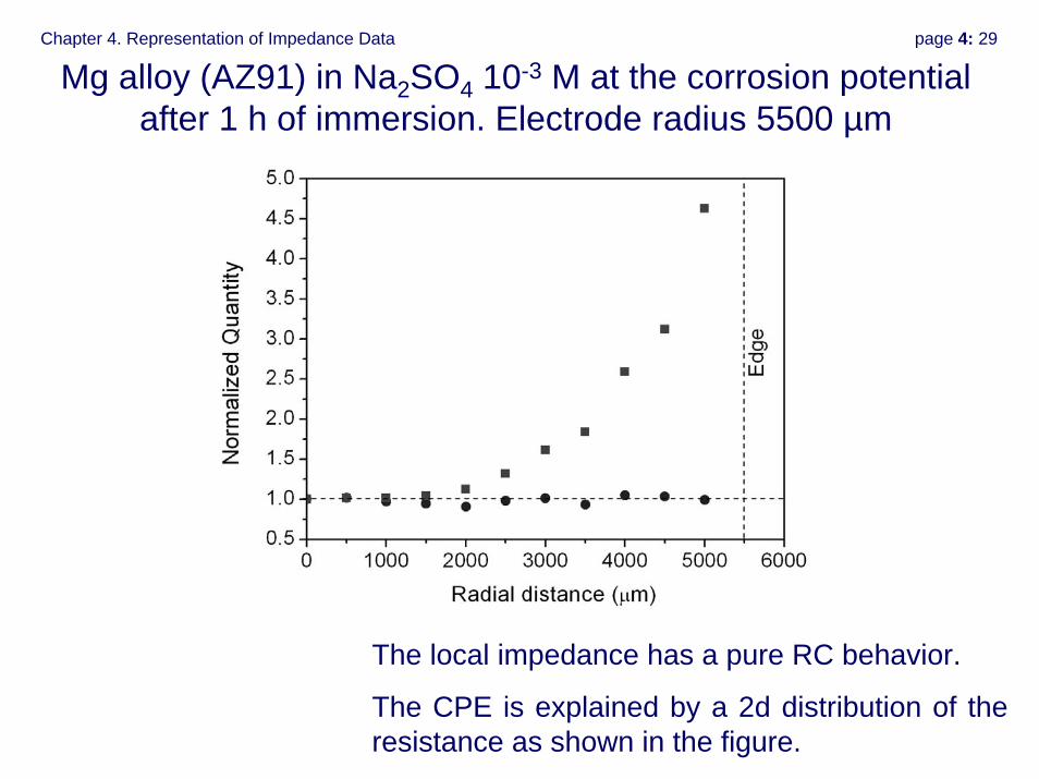
Mg alloy (AZ91) in Na2SO4 10-3 M at the corrosion potential after 1 h of immersion. Electrode radius 5500 µm.
Global impedance
Global impedance analyzed with a CPE (α = 0.91). Only the HF loop of the diagram is analyzed
J.-B. Jorcin, M. E. Orazem, N. Pébère, and B. Tribollet, Electrochimica Acta, 51 (2006), 1473-1479.

Chapter 4. Representation of Impedance Data page 4: 28
Local impedance
α = 1 to 0.92
Chapter 4. Representation of Impedance Data page 4: 29
Mg alloy (AZ91) in Na2SO4 10-3 M at the corrosion potential after 1 h of immersion. Electrode radius 5500 µm
The local impedance has a pure RC behavior.
The CPE is explained by a 2d distribution of the resistance as shown in the figure.Local impedance
Chapter 4. Representation of Impedance Data page 4: 30
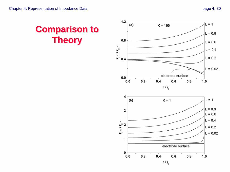
Comparison to Comparison to TheoryTheory
Chapter 4. Representation of Impedance Data page 4: 31
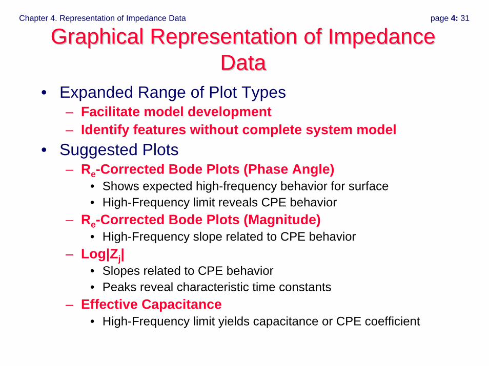
Graphical Representation of Impedance Graphical Representation of Impedance DataData
• Expanded Range of Plot Types– Facilitate model development– Identify features without complete system model
• Suggested Plots– Re-Corrected Bode Plots (Phase Angle)
• Shows expected high-frequency behavior for surface• High-Frequency limit reveals CPE behavior
– Re-Corrected Bode Plots (Magnitude) • High-Frequency slope related to CPE behavior
– Log|Zj|• Slopes related to CPE behavior• Peaks reveal characteristic time constants
– Effective Capacitance• High-Frequency limit yields capacitance or CPE coefficient
Chapter 4. Representation of Impedance Data page 4: 32
Plots based on Deterministic ModelsPlots based on Deterministic Models

Chapter 4. Representation of Impedance Data page 4: 33
Convective Diffusion to a RDEConvective Diffusion to a RDElow-frequency asymptote
Reduction of Fe(CN)63- on a Pt Disk, i/ilim = 1/2
0 50 100 150 200 2500
-50
-100
120 rpm 600 rpm 1200 rpm 2400 rpm
Z j / Ω
Zr / Ω
Chapter 4. Representation of Impedance Data page 4: 34
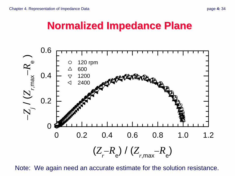
Normalized Impedance PlaneNormalized Impedance Plane
0 0.2 0.4 0.6 0.8 1.0 1.20
0.2
0.4
0.6 120 rpm 600 1200 2400
−Zj /
(Zr,m
ax−R
e )
(Zr−Re) / (Zr,max−Re)Note: We again need an accurate estimate for the solution resistance.
Chapter 4. Representation of Impedance Data page 4: 35
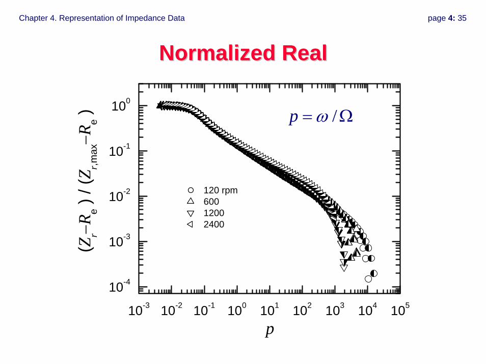
Normalized RealNormalized Real
10-3 10-2 10-1 100 101 102 103 104 105
10-4
10-3
10-2
10-1
100
120 rpm 600 1200 2400
(Zr−R
e ) /
(Zr,m
ax−R
e )
p
/p ω= Ω
Chapter 4. Representation of Impedance Data page 4: 36
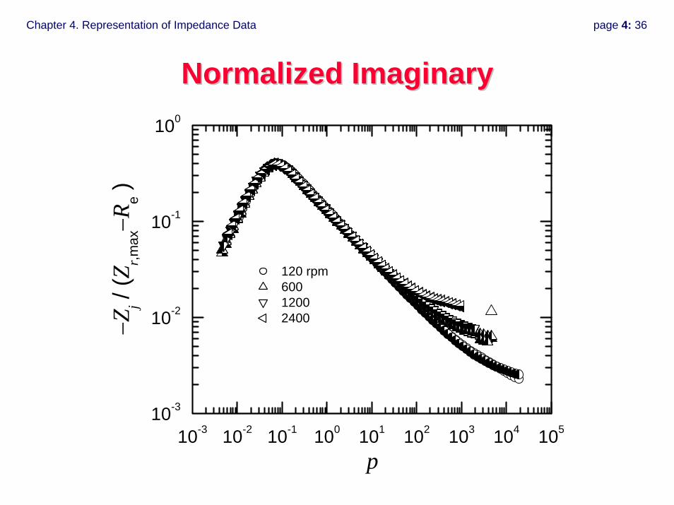
Normalized ImaginaryNormalized Imaginary
10-3 10-2 10-1 100 101 102 103 104 10510-3
10-2
10-1
100
120 rpm 600 1200 2400
−Zj /
(Zr,m
ax−R
e )
p

Chapter 4. Representation of Impedance Data page 4: 37
0 0.1 0.2 0.3 0.4 0.5
0
0.2
0.4
0.6
0.8
1.0 120 rpm 600 1200 2400
(Zr−R
e ) /
(Zr,m
ax−R
e )
−pZj / (Zr,max−Re )
Straight line at low frequencyStraight line at low frequency
Tribollet, Newman, and Smyrl, JES 135 (1988), 134-138.
Chapter 4. Representation of Impedance Data page 4: 38
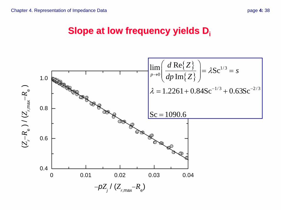
Slope at low frequency yields DSlope at low frequency yields Dii
0 0.01 0.02 0.03 0.040.4
0.6
0.8
1.0
(Zr−R
e ) /
(Zr,m
ax−R
e )
−pZj / (Zr,max−Re)
{ }{ }
1/ 30
1/ 3 2 / 3
Relim ScIm
1.2261 0.84Sc 0.63Sc
Sc 1090.6
p
d Zs
dp Zλ
λ
→
− −
⎛ ⎞= =⎜ ⎟⎜ ⎟
⎝ ⎠= + +
=
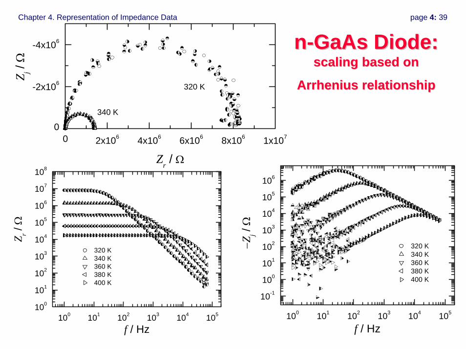
Chapter 4. Representation of Impedance Data page 4: 39
100 101 102 103 104 105
10-1
100
101
102
103
104
105
106
320 K 340 K 360 K 380 K 400 K
−Zj /
Ω
f / Hz
nn--GaAsGaAs Diode:Diode:scaling based on scaling based on
Arrhenius relationshipArrhenius relationship
0 2x10⁶ 4x10⁶ 6x10⁶ 8x10⁶ 1x1070
-2x10⁶
-4x10⁶
340 K
320 K
Z j / Ω
Zr / Ω
100 101 102 103 104 105100
101
102
103
104
105
106
107
108
320 K 340 K 360 K 380 K 400 K
Z r / Ω
f / Hz
Chapter 4. Representation of Impedance Data page 4: 40
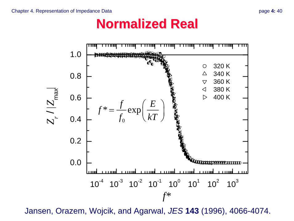
10-4 10-3 10-2 10-1 100 101 102 103
0.0
0.2
0.4
0.6
0.8
1.0 320 K 340 K 360 K 380 K 400 K
Z r / |Z
max
|
f*
Normalized RealNormalized Real
0
* expf Eff kT
⎛ ⎞= ⎜ ⎟⎝ ⎠
Jansen, Orazem, Wojcik, and Agarwal, JES 143 (1996), 4066-4074.
Chapter 4. Representation of Impedance Data page 4: 41
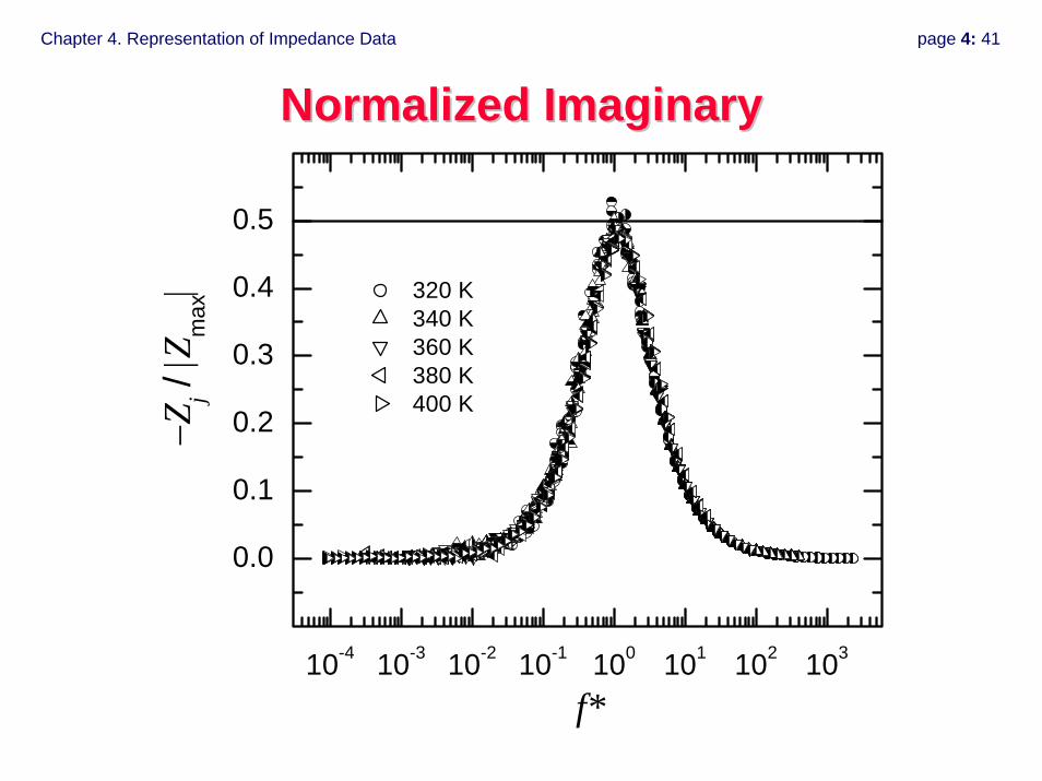
Normalized ImaginaryNormalized Imaginary
10-4 10-3 10-2 10-1 100 101 102 103
0.0
0.1
0.2
0.3
0.4
0.5
320 K 340 K 360 K 380 K 400 K
−Zj /
|Zm
ax|
f*
Chapter 4. Representation of Impedance Data page 4: 42
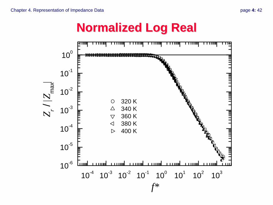
Normalized Log RealNormalized Log Real
10-4 10-3 10-2 10-1 100 101 102 10310-6
10-5
10-4
10-3
10-2
10-1
100
320 K 340 K 360 K 380 K 400 K
Z r / |Z
max
|
f*
Chapter 4. Representation of Impedance Data page 4: 43
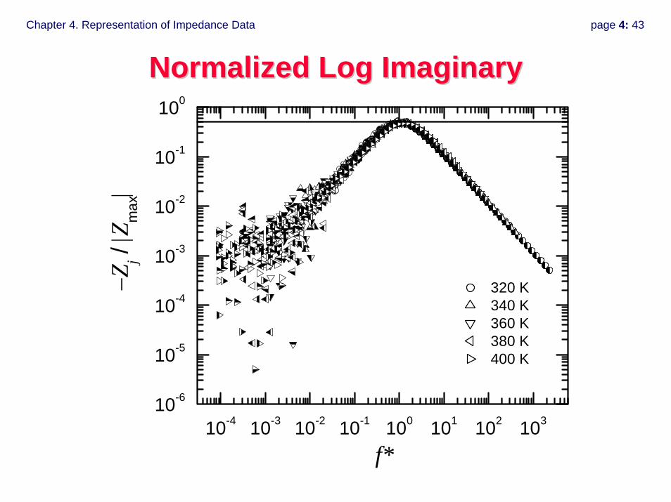
Normalized Log ImaginaryNormalized Log Imaginary
10-4 10-3 10-2 10-1 100 101 102 10310-6
10-5
10-4
10-3
10-2
10-1
100
320 K 340 K 360 K 380 K 400 K
−Zj /
|Zm
ax|
f*
Chapter 4. Representation of Impedance Data page 4: 44
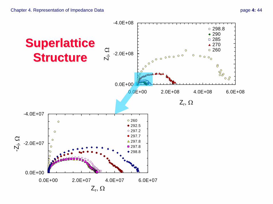
SuperlatticeSuperlatticeStructureStructure
-4.0E+08
-2.0E+08
0.0E+000.0E+00 2.0E+08 4.0E+08 6.0E+08
Zr, ΩZ j
, Ω
298.8290285270260
-4.0E+07
-2.0E+07
0.0E+000.0E+00 2.0E+07 4.0E+07 6.0E+07
Zr, Ω
-Zj,
Ω
260292.5297.2297.7297.8297.8298.8
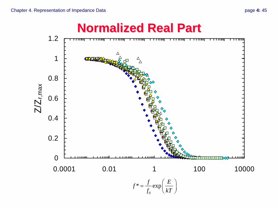
Chapter 4. Representation of Impedance Data page 4: 45
0
0.2
0.4
0.6
0.8
1
1.2
0.0001 0.01 1 100 10000
Z/Z r
,max
Normalized Real PartNormalized Real Part
0
* expf Eff kT
⎛ ⎞= ⎜ ⎟⎝ ⎠
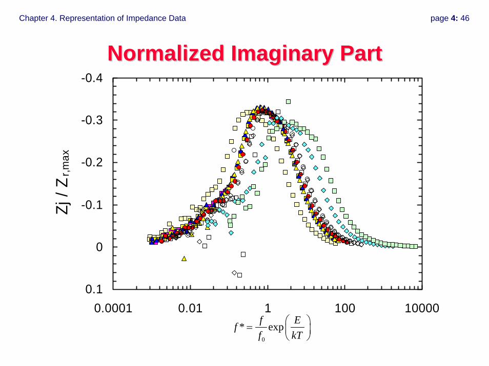
Chapter 4. Representation of Impedance Data page 4: 46
Normalized Imaginary PartNormalized Imaginary Part-0.4
-0.3
-0.2
-0.1
0
0.10.0001 0.01 1 100 10000
Zj /
Zr,m
ax
0
* expf Eff kT
⎛ ⎞= ⎜ ⎟⎝ ⎠
Chapter 4. Representation of Impedance Data page 4: 47
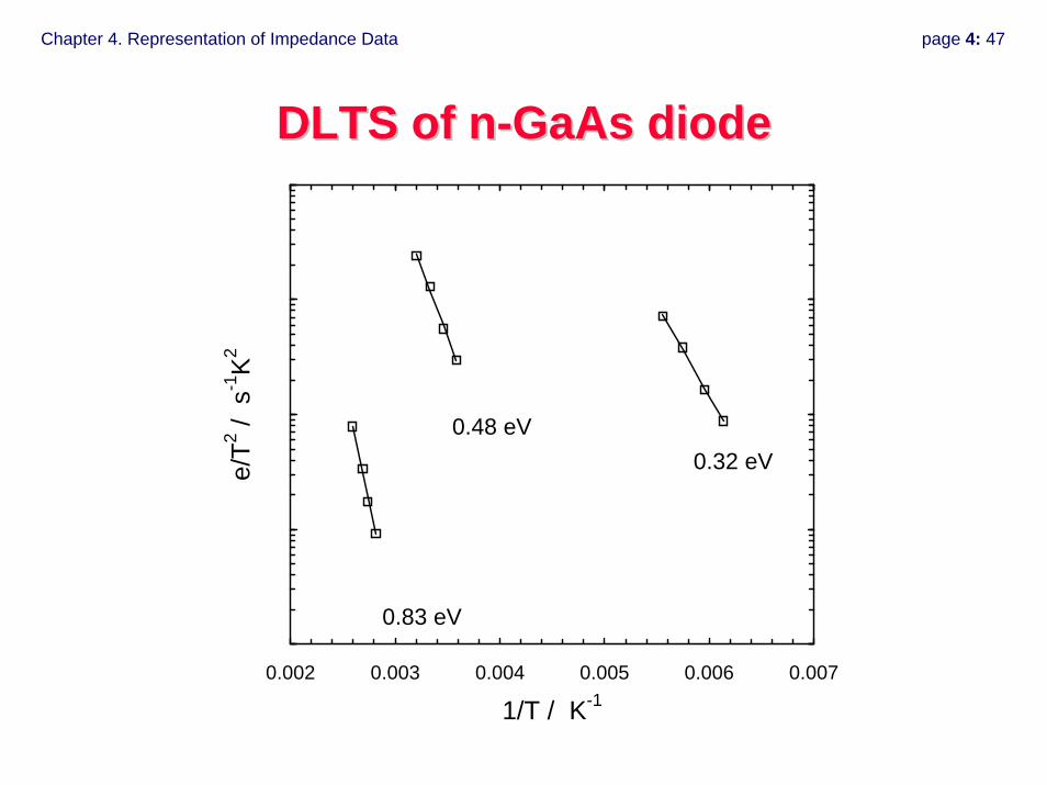
DLTS of DLTS of nn--GaAsGaAs diodediode
0.002 0.003 0.004 0.005 0.006 0.007
1/T / K-1
e/T2 /
s-1
K2
0.83 eV
0.48 eV0.32 eV
Chapter 4. Representation of Impedance Data page 4: 48
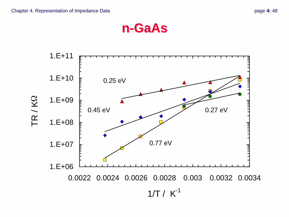
nn--GaAsGaAs
1.E+06
1.E+07
1.E+08
1.E+09
1.E+10
1.E+11
0.0022 0.0024 0.0026 0.0028 0.003 0.0032 0.0034
1/T / K-1
TR /
K
0.77 eV
0.45 eV
0.25 eV
0.27 eV
Chapter 4. Representation of Impedance Data page 4: 49
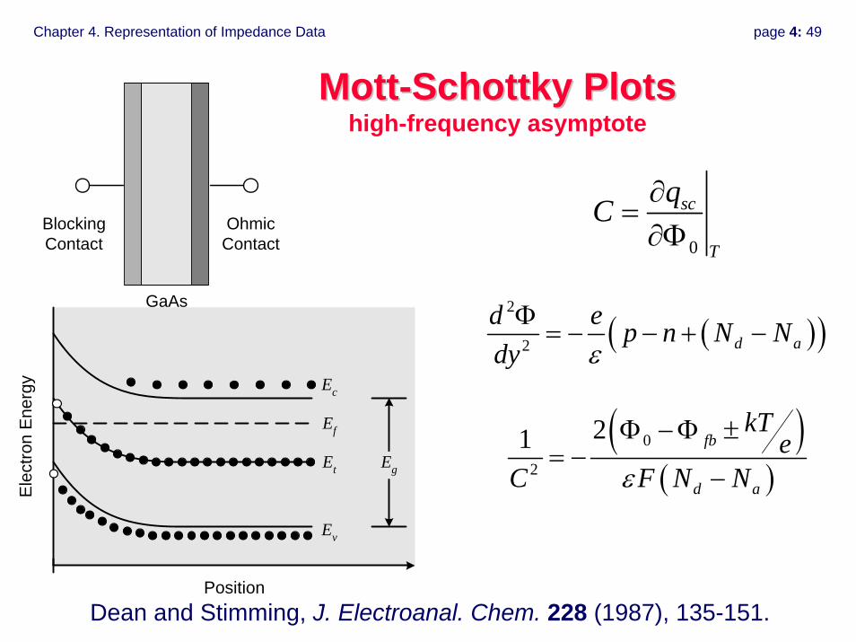
MottMott--SchottkySchottky PlotsPlotshigh-frequency asymptote
0
sc
T
qC ∂=
∂Φ
( )( )2
2 d ad e p n N Ndy ε
Φ= − − + −
( )( )
0
2
21 fb
d a
kTe
C F N Nε
Φ − Φ ±= −
−
Ef
Ec
Ev
Et Eg
Position
Elec
tron
Ener
gy
GaAs
BlockingContact
OhmicContact
Dean and Stimming, J. Electroanal. Chem. 228 (1987), 135-151.

Chapter 4. Representation of Impedance Data page 4: 50
C as a function of PotentialC as a function of Potentialintrinsic semiconductor
-0.4 -0.2 0 0.2 0.410-8
10-7
10-6
10-5
10-4
10-3
C
/ μF
cm
-2
(Φ-Φfb) / V
Chapter 4. Representation of Impedance Data page 4: 51
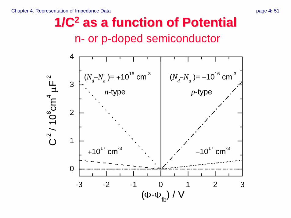
1/C1/C22 as a function of Potentialas a function of Potentialn- or p-doped semiconductor
-3 -2 -1 0 1 2 3
0
1
2
3
4
p-typen-type
−1017 cm-3 +1017 cm-3
(Nd−Na )= +1016 cm-3 (Nd−Na )= −1016 cm-3
C-2 /
108 cm
4 μF-2
(Φ-Φfb) / V

Chapter 4. Representation of Impedance Data page 4: 52
GaAsGaAs--SchottkySchottky DiodeDiode
-3 -2 -1 0 1 20
2
4
6
8
C -2
/ nF
-2
Potential / V

Chapter 4. Representation of Impedance Data page 4: 53
Choice of RepresentationChoice of Representation
• Plotting approaches are useful to show governing phenomena
• Complement to regression of detailed models• Sensitive analysis requires use of properly weighted
complex nonlinear regression

Chapter 4. Representation of Impedance Data page 4: 54
Chapter 5. Development of Process Models page 5: 1
Electrochemical Impedance Electrochemical Impedance SpectroscopySpectroscopy
Chapter 5. Development of Process ModelsChapter 5. Development of Process Models
• Use of Circuits to guide development• Develop models from physical grounds• Model case study• Identify correspondence between physical models and
electrical circuit analogues• Account for mass transfer
© Mark E. Orazem, 2000-2008. All rights reserved.

Chapter 5. Development of Process Models page 5: 2
Use circuits to create frameworkUse circuits to create framework
Chapter 5. Development of Process Models page 5: 3
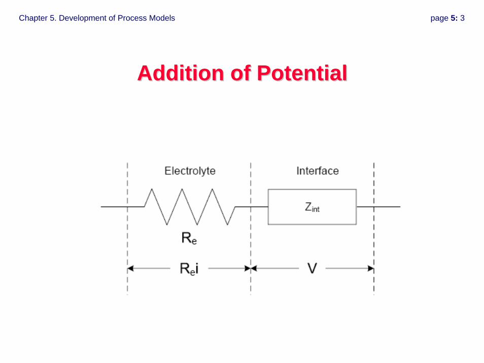
Addition of PotentialAddition of Potential
Chapter 5. Development of Process Models page 5: 4
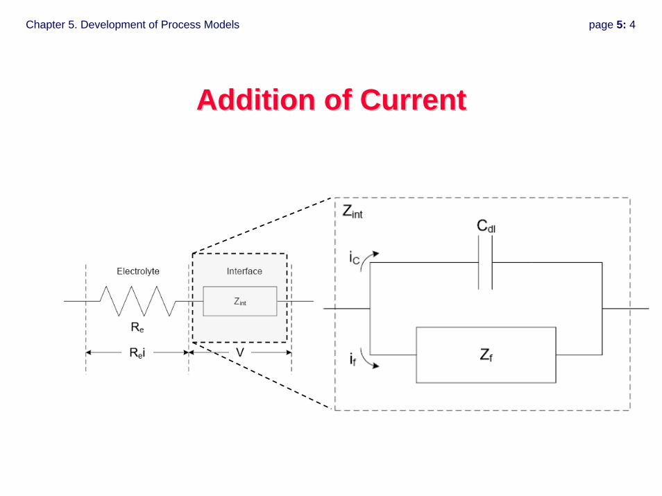
Addition of CurrentAddition of Current
Chapter 5. Development of Process Models page 5: 5
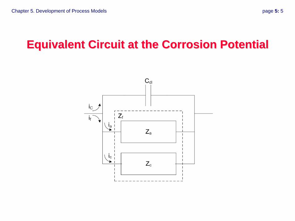
Equivalent Circuit at the Corrosion PotentialEquivalent Circuit at the Corrosion Potential
Chapter 5. Development of Process Models page 5: 6
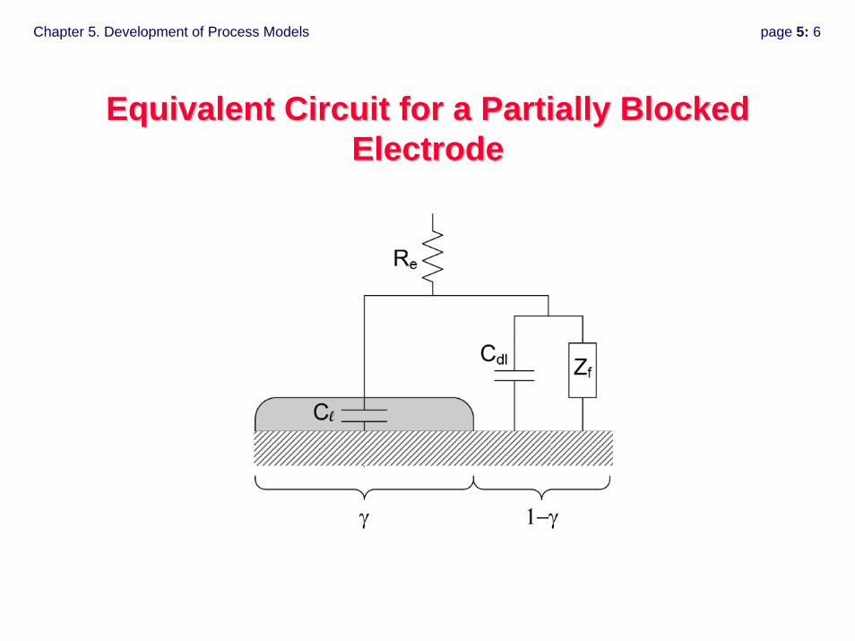
Equivalent Circuit for a Partially Blocked Equivalent Circuit for a Partially Blocked ElectrodeElectrode
Chapter 5. Development of Process Models page 5: 7
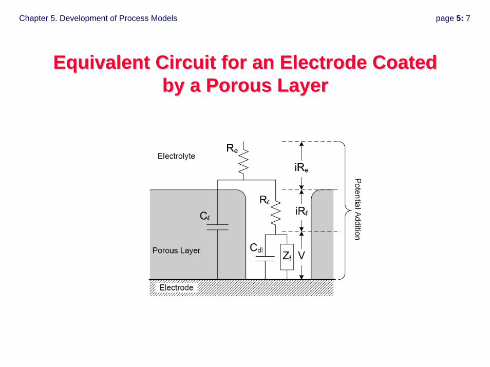
Equivalent Circuit for an Electrode Coated Equivalent Circuit for an Electrode Coated by a Porous Layerby a Porous Layer
Chapter 5. Development of Process Models page 5: 8
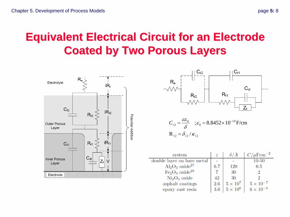
Equivalent Electrical Circuit for an Electrode Equivalent Electrical Circuit for an Electrode Coated by Two Porous LayersCoated by Two Porous Layers
1402 0
2 2 2
; 8.8452 10 F/cm
R /
C εεε
δδ κ
−= = ×
=
Chapter 5. Development of Process Models page 5: 9
Use kinetic models to determine Use kinetic models to determine expressions for the interfacial impedanceexpressions for the interfacial impedance
Chapter 5. Development of Process Models page 5: 10
ApproachApproachidentify reaction mechanismwrite expression for steady state current contributionswrite expression for sinusoidal steady statesum current contributionsaccount for charging currentaccount for ohmic potential dropaccount for mass transfercalculate impedance
√√√√√√√√
Chapter 5. Development of Process Models page 5: 11
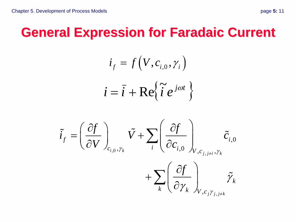
General Expression for General Expression for FaradaicFaradaic CurrentCurrent
,0 ,
,
,0, ,0 , ,
,
i k j j i k
j j j k
f iic i V c
kk k V c
f fi V cV c
f
γ γ
γ
γγ
≠
≠
⎛ ⎞∂ ∂⎛ ⎞= + ⎜ ⎟⎜ ⎟ ⎜ ⎟∂ ∂⎝ ⎠ ⎝ ⎠
⎛ ⎞∂+ ⎜ ⎟∂⎝ ⎠
∑
∑
( ),0, ,f i ii f V c γ=
{ }tjeiii ω~Re+=
Chapter 5. Development of Process Models page 5: 12
Reactions ConsideredReactions Considered
• Dependent on Potential• Dependent on Potential and Mass Transfer• Dependent on Potential, Mass Transfer, and Surface
Coverage• Coupled Reactions
Chapter 5. Development of Process Models page 5: 13
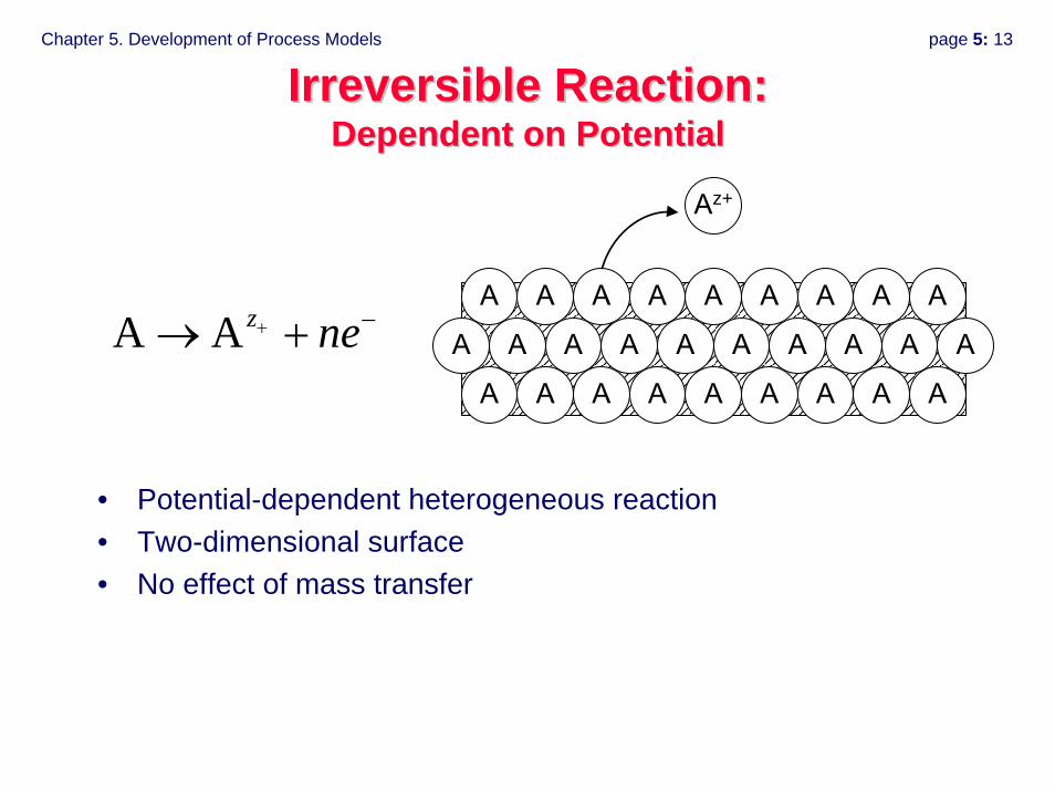
Irreversible Reaction: Irreversible Reaction: Dependent on PotentialDependent on Potential
A A z ne+ −→ +
z+
• Potential-dependent heterogeneous reaction• Two-dimensional surface• No effect of mass transfer
Chapter 5. Development of Process Models page 5: 14
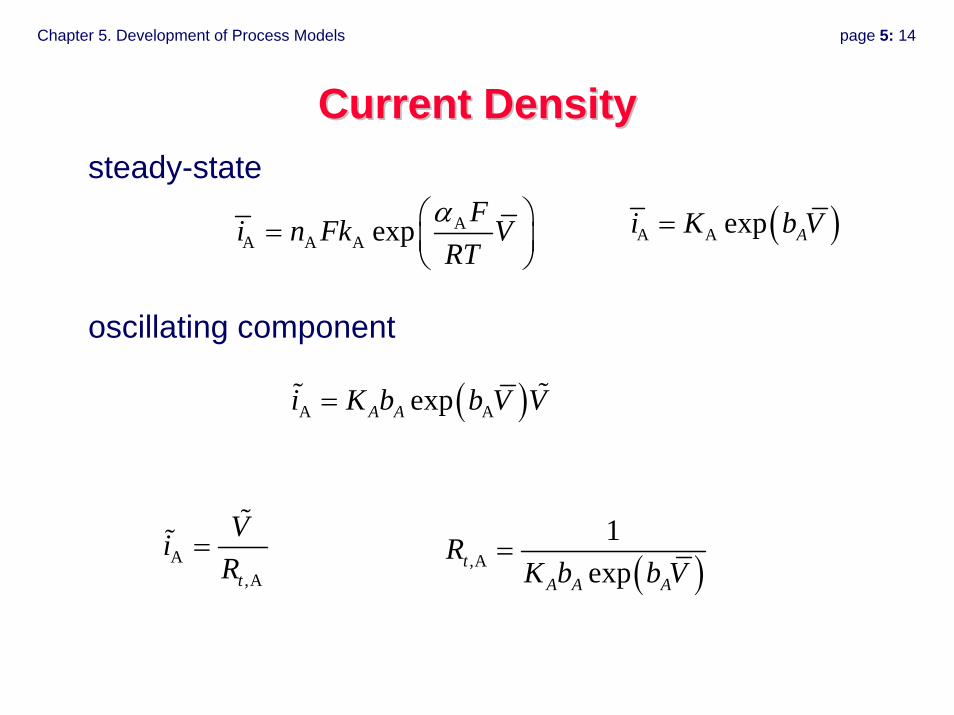
Current DensityCurrent Density
A,At
ViR
=( ),A
1expt
A A A
RK b b V
=
AA A A exp Fi n Fk V
RTα⎛ ⎞= ⎜ ⎟⎝ ⎠
steady-state
( )A AexpA Ai K b b V V=
oscillating component
( )A A exp Ai K b V=

Chapter 5. Development of Process Models page 5: 15
f dl
f dl
dVi i Cdt
i i j C Vω
= +
= +
Charging CurrentCharging Current
low frequency
high frequency
,A
,A
1
dlt
dlt
Vi j C VR
V j CR
ω
ω
= +
⎛ ⎞= +⎜ ⎟⎜ ⎟
⎝ ⎠
,A
,A1t
t dl
RVi j R Cω=
+
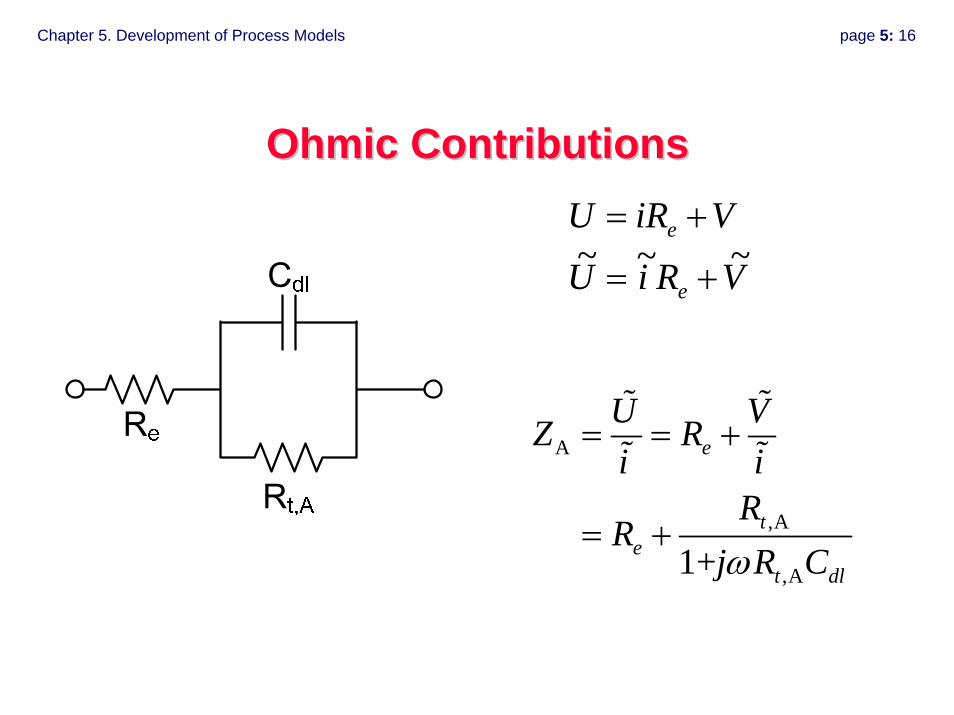
Chapter 5. Development of Process Models page 5: 16
Ohmic ContributionsOhmic Contributions
VRiU
ViRU
e
e~~~ +=
+=
A
,A
,A1+
e
te
t dl
U VZ Ri i
RR
j R Cω
= = +
= +
Chapter 5. Development of Process Models page 5: 17
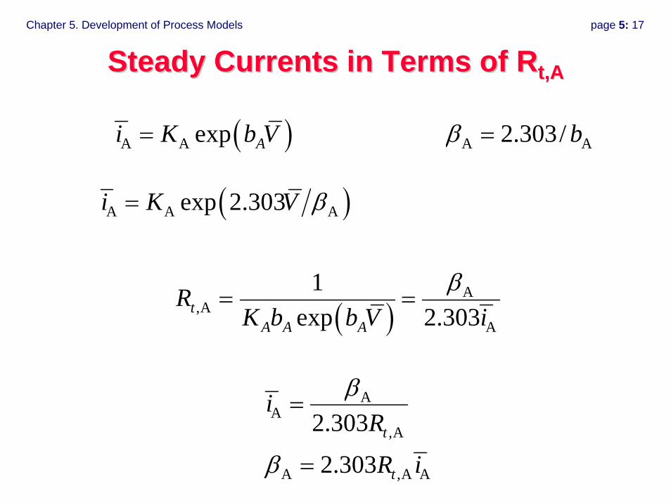
( )A A Aexp 2.303i K V β=
A A2.303/ bβ =
( )A
,AA
1exp 2.303t
A A A
RK b b V i
β= =
AA
,A
A ,A A
2.303
2.303t
t
iR
R i
β
β
=
=
( )A A exp Ai K b V=
Steady Currents in Terms of Steady Currents in Terms of RRt,At,A
Chapter 5. Development of Process Models page 5: 18
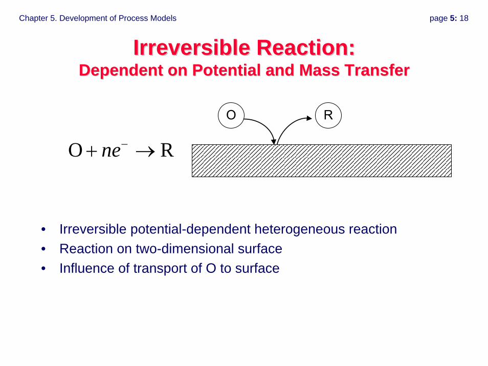
Irreversible Reaction: Irreversible Reaction: Dependent on Potential and Mass TransferDependent on Potential and Mass Transfer
O Rne−+ →
• Irreversible potential-dependent heterogeneous reaction• Reaction on two-dimensional surface• Influence of transport of O to surface
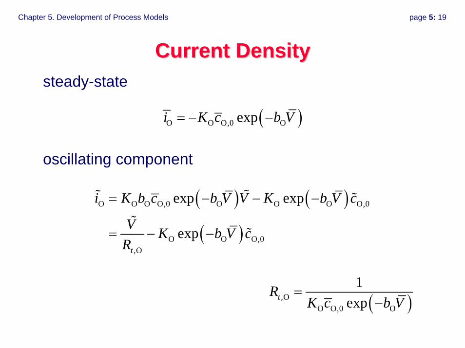
Chapter 5. Development of Process Models page 5: 19
Current DensityCurrent Density
( ),OO O,0 O
1exptR
K c b V=
−
( )O O O,0 Oexpi K c b V= − −
steady-state
( ) ( )
( )
O O O O,0 O O O O,0
O O O,0,O
exp exp
expt
i K b c b V V K b V c
V K b V cR
= − − −
= − −
oscillating component
Chapter 5. Development of Process Models page 5: 20
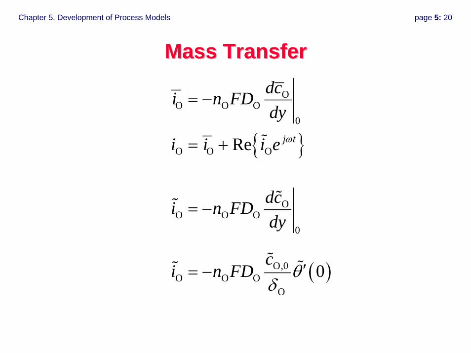
Mass TransferMass Transfer
{ }
OO O O
0
O O ORe j t
dci n FDdy
i i i e ω
= −
= +
OO O O
0
dci n FDdy
= −
( )O,0O O O
O
0c
i n FD θδ
′= −

Chapter 5. Development of Process Models page 5: 21
Combine ExpressionsCombine Expressions
( )O O O O,0,O
expt
Vi K b V cR
= −
( )O O
O,0O O 0
icn FD
δθ
= −′
Chapter 5. Development of Process Models page 5: 22
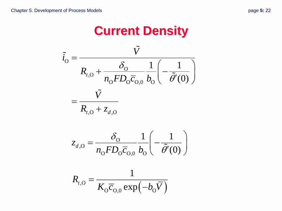
Current DensityCurrent Density
OO
,OO O O,0 O
,O ,O
1 1(0)t
t d
ViR
n FD c b
VR z
δθ
=⎛ ⎞
+ −⎜ ⎟′⎝ ⎠
=+
O,O
O O O,0 O
1 1(0)dz
n FD c bδ
θ⎛ ⎞
= −⎜ ⎟′⎝ ⎠
( ),OO O,0 O
1exptR
K c b V=
−
Chapter 5. Development of Process Models page 5: 23
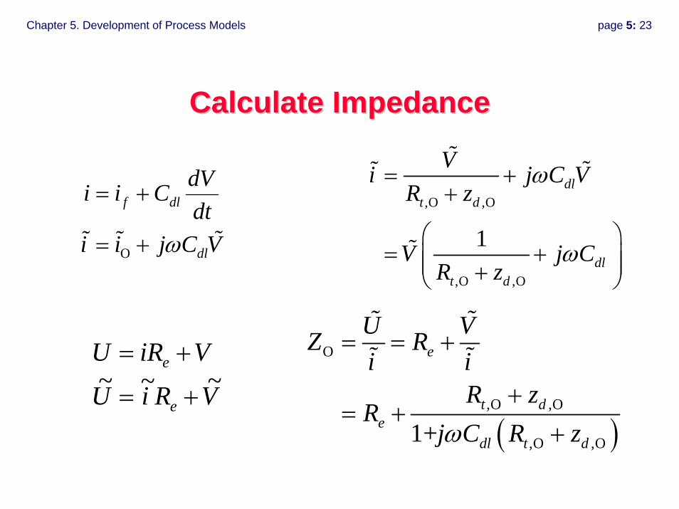
Calculate ImpedanceCalculate Impedance
O
f dl
dl
dVi i Cdt
i i j C Vω
= +
= +
,O ,O
,O ,O
1
dlt d
dlt d
Vi j C VR z
V j CR z
ω
ω
= ++
⎛ ⎞= +⎜ ⎟⎜ ⎟+⎝ ⎠
VRiU
ViRU
e
e~~~ +=
+=
( )
O
,O ,O
,O ,O1+
e
t de
dl t d
U VZ Ri i
R zR
j C R zω
= = +
+= +
+
Chapter 5. Development of Process Models page 5: 24
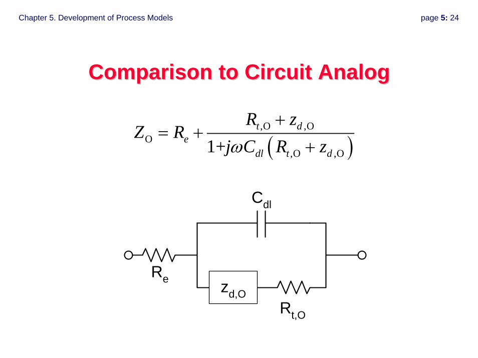
Comparison to Circuit AnalogComparison to Circuit Analog
Cdl
Re
Rt,O
zd,O
( ),O ,O
O,O ,O1+
t de
dl t d
R zZ R
j C R zω+
= ++
Chapter 5. Development of Process Models page 5: 25
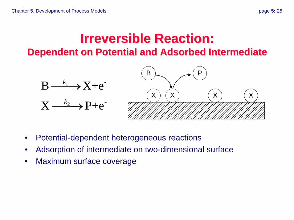
Irreversible Reaction: Irreversible Reaction: Dependent on Potential and Adsorbed IntermediateDependent on Potential and Adsorbed Intermediate
1
2
-
-
B X+eX P+e
k
k
⎯⎯→
⎯⎯→
• Potential-dependent heterogeneous reactions• Adsorption of intermediate on two-dimensional surface• Maximum surface coverage
B
X X XX
P
Chapter 5. Development of Process Models page 5: 26
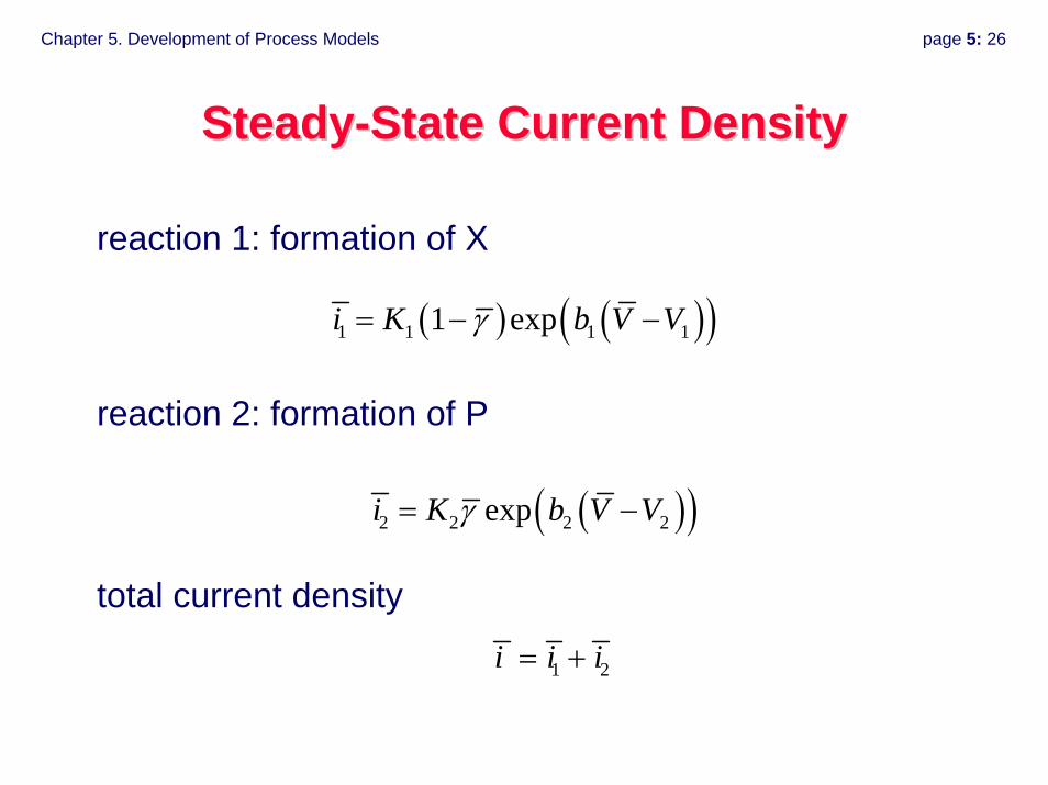
SteadySteady--State Current DensityState Current Density
( ) ( )( )1 1 1 11 expi K b V Vγ= − −
reaction 1: formation of X
reaction 2: formation of P
( )( )2 2 2 2expi K b V Vγ= −
total current density
1 2i i i= +
Chapter 5. Development of Process Models page 5: 27
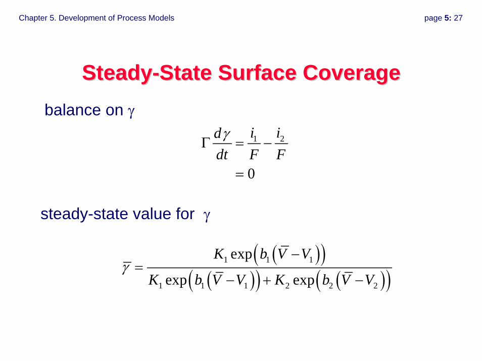
SteadySteady--State Surface CoverageState Surface Coverage
1 2
0
i iddt F Fγ
Γ = −
=
balance on γ
( )( )( )( ) ( )( )
1 1 1
1 1 1 2 2 2
exp
exp exp
K b V V
K b V V K b V Vγ
−=
− + −
steady-state value for γ
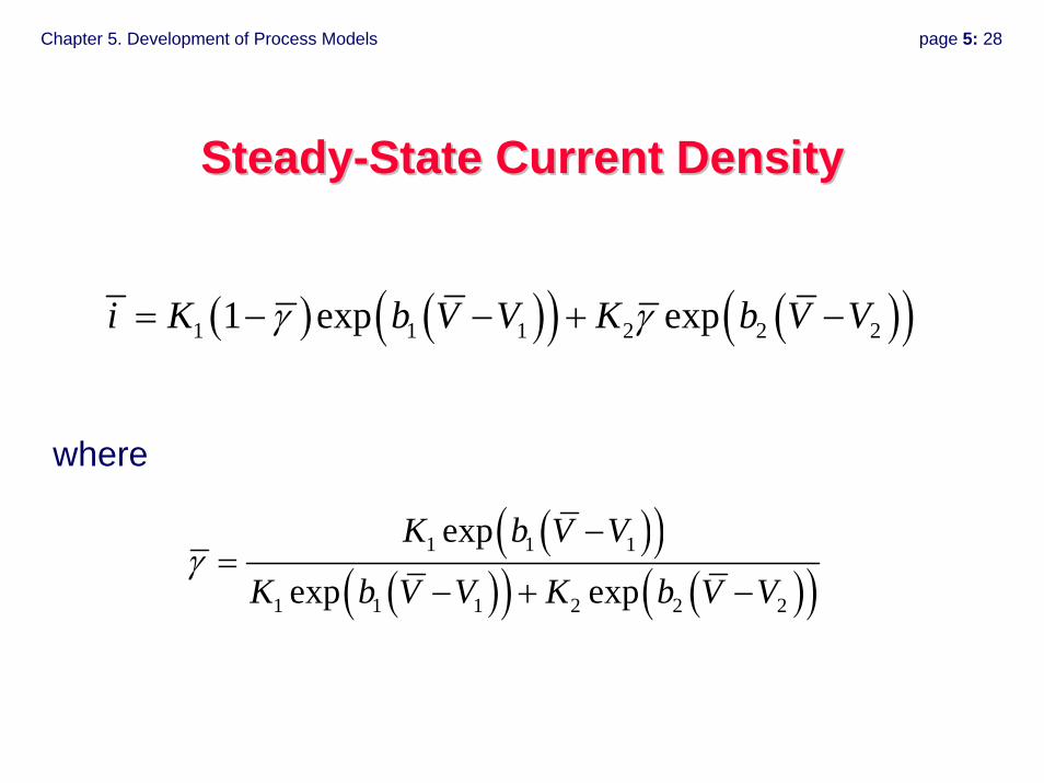
Chapter 5. Development of Process Models page 5: 28
SteadySteady--State Current DensityState Current Density
( ) ( )( ) ( )( )1 1 1 2 2 21 exp expi K b V V K b V Vγ γ= − − + −
( )( )( )( ) ( )( )
1 1 1
1 1 1 2 2 2
exp
exp exp
K b V V
K b V V K b V Vγ
−=
− + −
where
Chapter 5. Development of Process Models page 5: 29
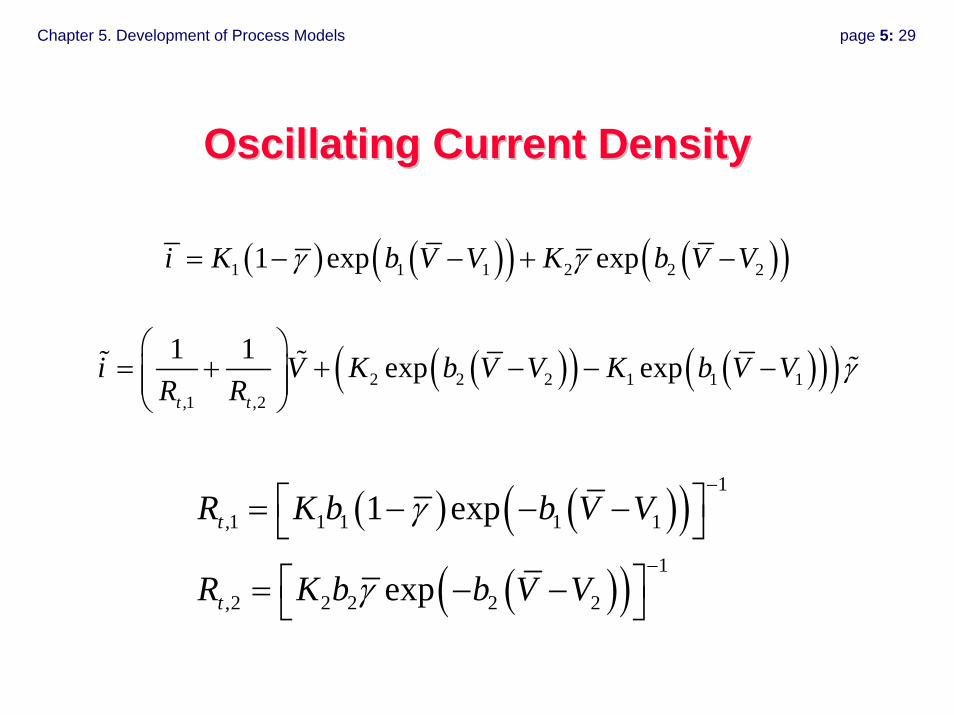
Oscillating Current DensityOscillating Current Density
( ) ( )( ) ( )( )1 1 1 2 2 21 exp expi K b V V K b V Vγ γ= − − + −
( )( ) ( )( )( )2 2 2 1 1 1,1 ,2
1 1 exp expt t
i V K b V V K b V VR R
γ⎛ ⎞
= + + − − −⎜ ⎟⎜ ⎟⎝ ⎠
( ) ( )( )( )( )
1
,1 1 1 1 1
1
,2 2 2 2 2
1 exp
exp
t
t
R K b b V V
R K b b V V
γ
γ
−
−
⎡ ⎤= − − −⎣ ⎦
⎡ ⎤= − −⎣ ⎦
Chapter 5. Development of Process Models page 5: 30
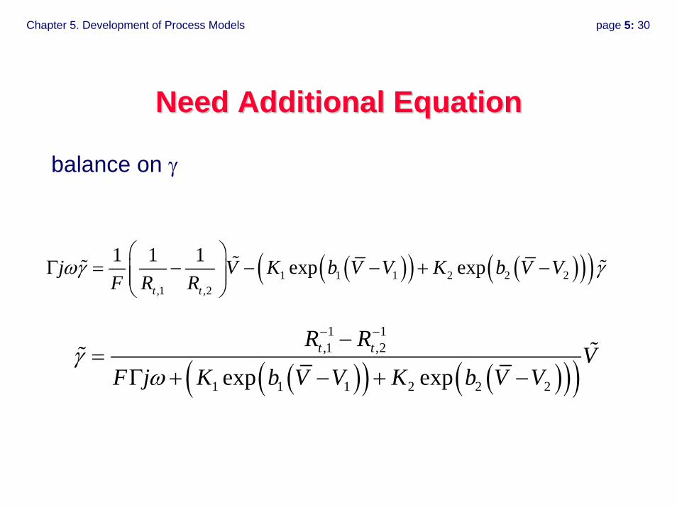
Need Additional EquationNeed Additional Equation
( )( ) ( )( )( )1 1 1 2 2 2,1 ,2
1 1 1 exp expt t
j V K b V V K b V VF R R
ωγ γ⎛ ⎞
Γ = − − − + −⎜ ⎟⎜ ⎟⎝ ⎠
balance on γ
( )( ) ( )( )( )1 1
,1 ,2
1 1 1 2 2 2exp expt tR R
VF j K b V V K b V V
γω
− −−=
Γ + − + −
Chapter 5. Development of Process Models page 5: 31
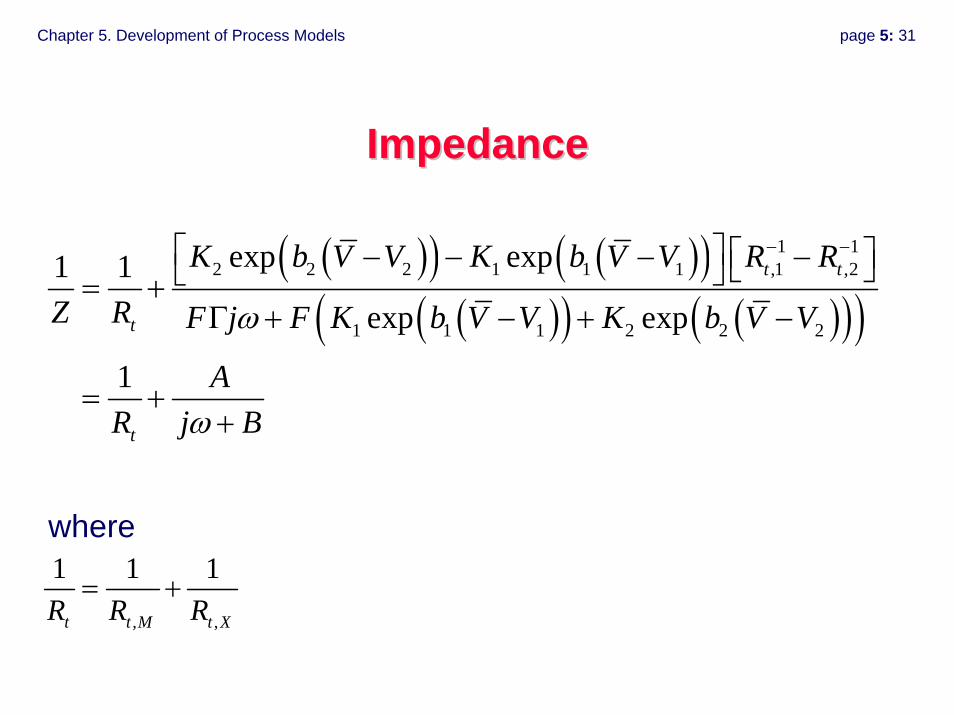
ImpedanceImpedance
( )( ) ( )( )( )( ) ( )( )( )
1 12 2 2 1 1 1 ,1 ,2
1 1 1 2 2 2
exp exp1 1exp exp
1
t t
t
t
K b V V K b V V R R
Z R F j F K b V V K b V V
AR j B
ω
ω
− −⎡ ⎤ ⎡ ⎤− − − −⎣ ⎦⎣ ⎦= +Γ + − + −
= ++
, ,
1 1 1
t t M t XR R R= +
where
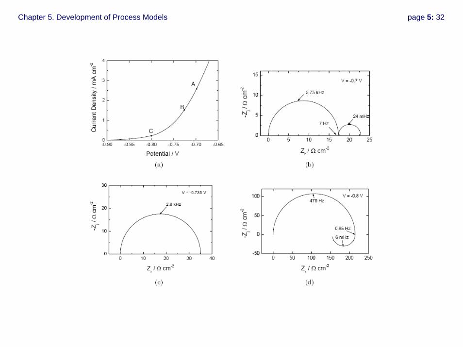
Chapter 5. Development of Process Models page 5: 32
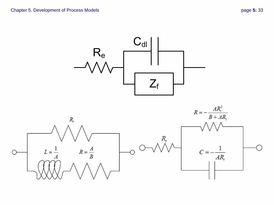
Chapter 5. Development of Process Models page 5: 33
Chapter 5. Development of Process Models page 5: 34
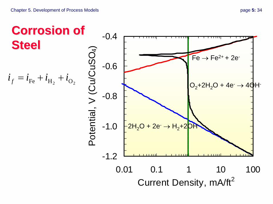
-1.2
-1.0
-0.8
-0.6
-0.4
0.01 0.1 1 10 100Current Density, mA/ft2
Pot
entia
l, V
(Cu/
CuS
O4)
Corrosion of Corrosion of SteelSteel
2H2O + 2e- → H2+2OH-
O2+2H2O + 4e- → 4OH-
Fe → Fe2+ + 2e-
22 OHFe iiii f ++=
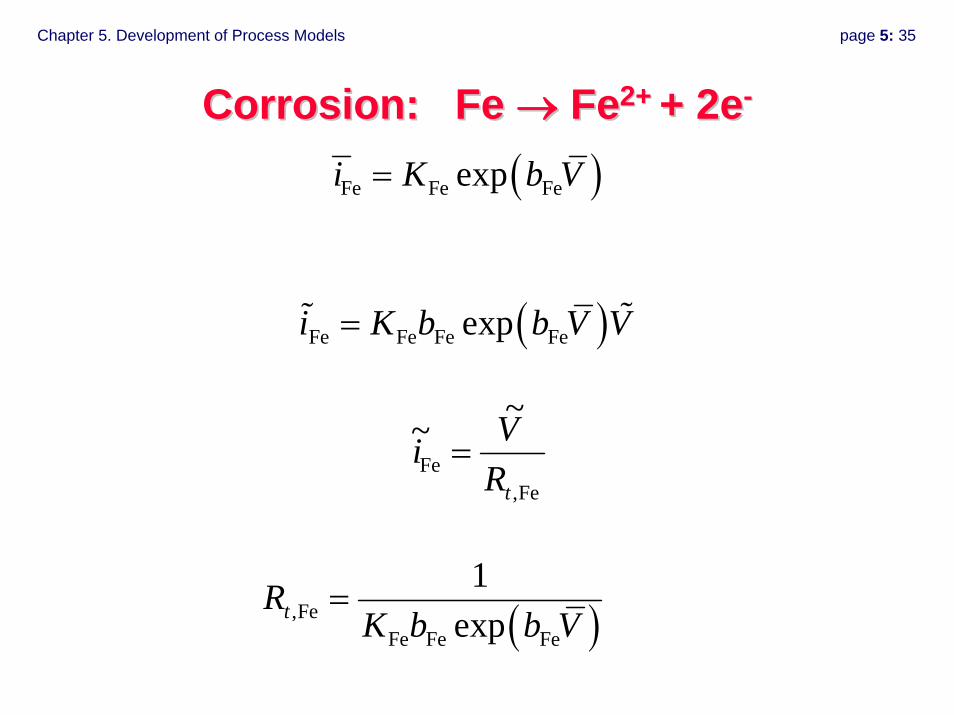
Chapter 5. Development of Process Models page 5: 35
Fe,Fe
~~tRVi =
( ),FeFe Fe Fe
1exptR
K b b V=
Corrosion: Fe Corrosion: Fe →→ FeFe2+ 2+ + 2e+ 2e--
( )Fe Fe Feexpi K b V=
( )Fe Fe Fe Feexpi K b b V V=
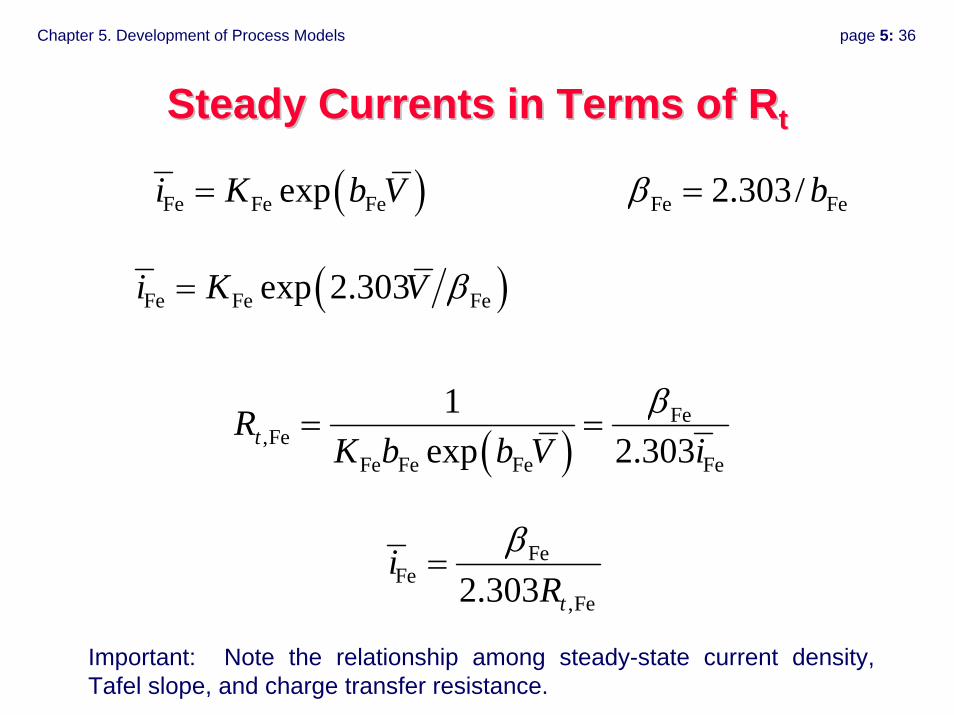
Chapter 5. Development of Process Models page 5: 36
Steady Currents in Terms of Steady Currents in Terms of RRtt
( )Fe Fe Feexp 2.303i K V β=
Fe Fe2.303/ bβ =
( )Fe
,FeFe Fe Fe Fe
1exp 2.303tR
K b b V iβ
= =
FeFe
,Fe2.303 t
iR
β=
( )Fe Fe Feexpi K b V=
Important: Note the relationship among steady-state current density, Tafel slope, and charge transfer resistance.
Chapter 5. Development of Process Models page 5: 37
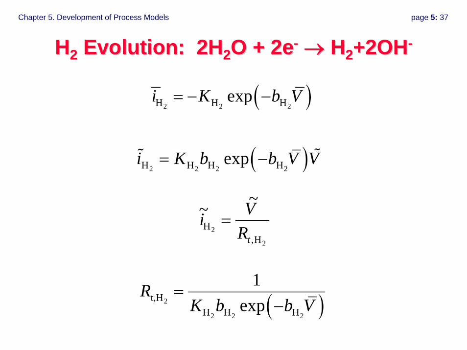
( )2 2 2H H Hexpi K b V= − −
( )2 2 2 2H H H Hexpi K b b V V= −
2
2H,
H
~~tRVi =
( )2
2 2 2
t,HH H H
1exp
RK b b V
=−
HH22 Evolution: 2HEvolution: 2H22O + 2eO + 2e-- →→ HH22+2OH+2OH--
Chapter 5. Development of Process Models page 5: 38
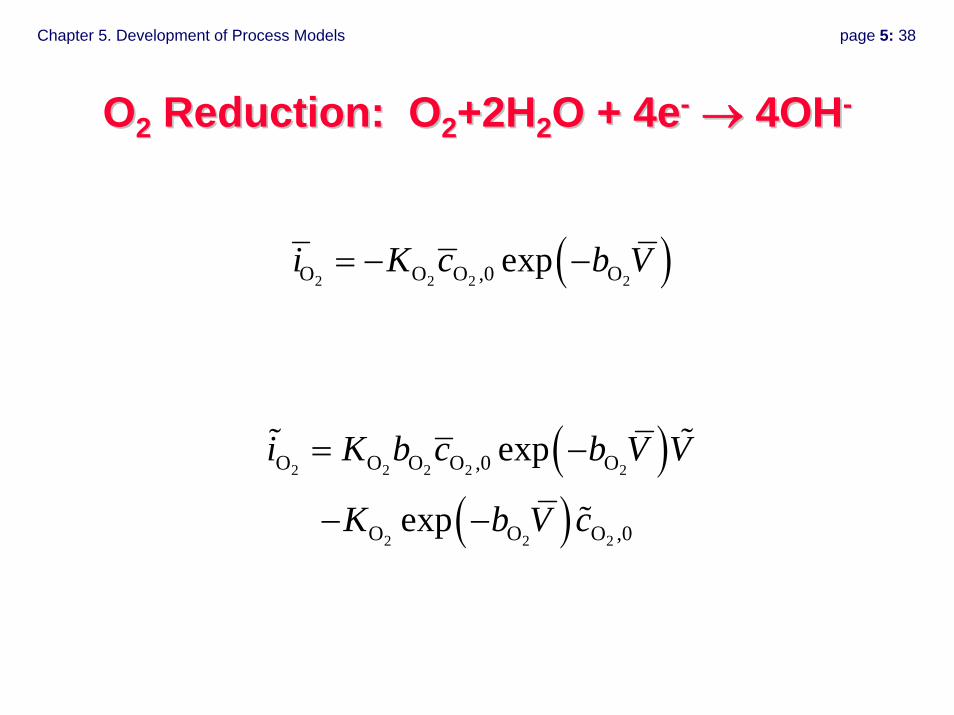
( )2 2 2 2O O O ,0 Oexpi K c b V= − −
( )( )
2 2 2 2 2
2 2 2
O O O O ,0 O
O O O ,0
exp
exp
i K b c b V V
K b V c
= −
− −
OO22 Reduction: OReduction: O22+2H+2H22O + 4eO + 4e-- →→ 4OH4OH--
Chapter 5. Development of Process Models page 5: 39
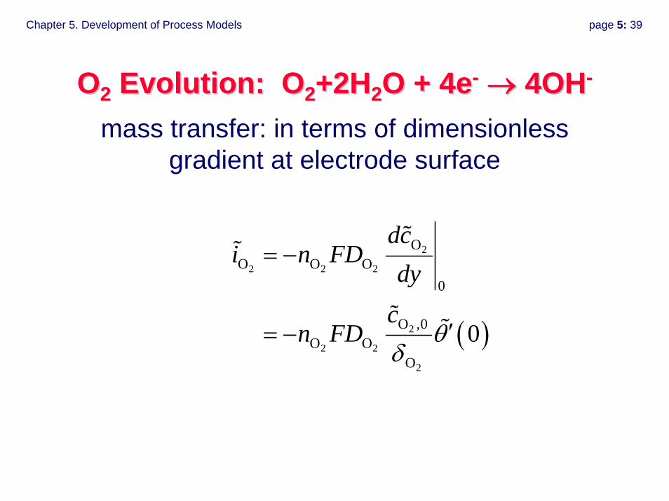
OO22 Evolution: OEvolution: O22+2H+2H22O + 4eO + 4e-- →→ 4OH4OH--
mass transfer: in terms of dimensionless gradient at electrode surface
( )
2
2 2 2
2
2 2
2
OO O O
0
O ,0O O
O
0
dci n FD
dyc
n FD θδ
= −
′= −
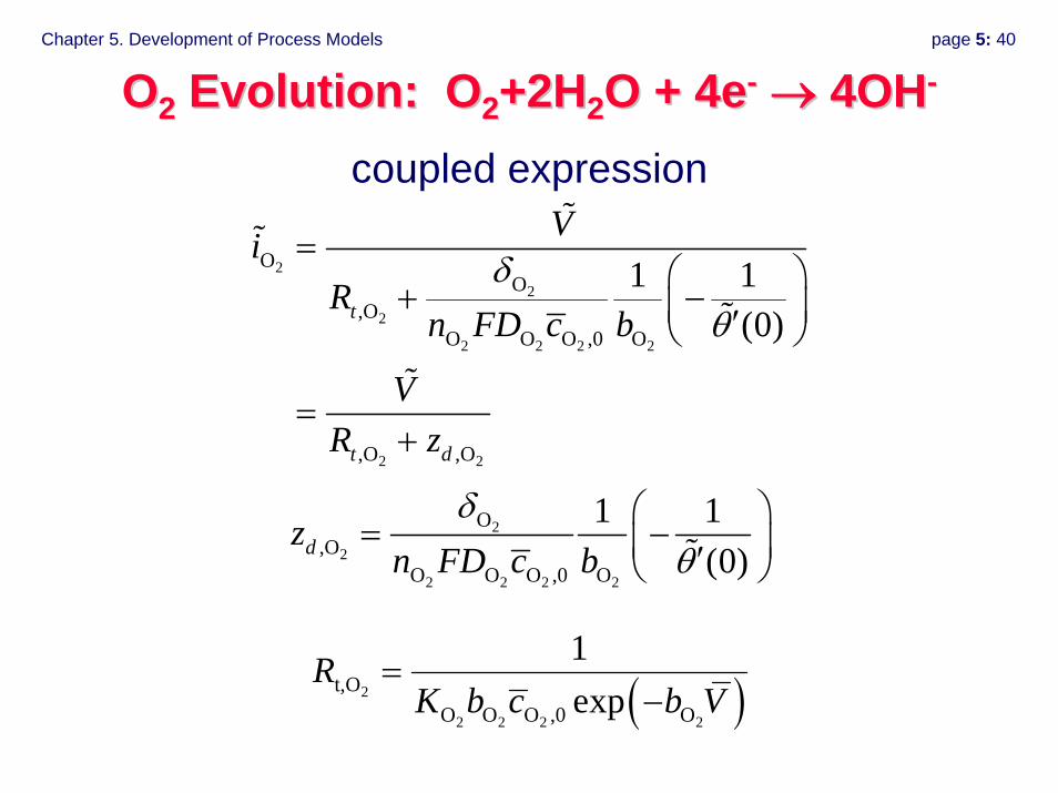
Chapter 5. Development of Process Models page 5: 40
22
2
2 2 2 2
2 2
OO
,OO O O ,0 O
,O ,O
1 1(0)t
t d
ViR
n FD c b
VR z
δθ
=⎛ ⎞
+ −⎜ ⎟′⎝ ⎠
=+
( )2
2 2 2 2
t,OO O O ,0 O
1exp
RK b c b V
=−
2
2
2 2 2 2
O,O
O O O ,0 O
1 1(0)dz
n FD c bδ
θ⎛ ⎞
= −⎜ ⎟′⎝ ⎠
OO22 Evolution: OEvolution: O22+2H+2H22O + 4eO + 4e-- →→ 4OH4OH--
coupled expression
Chapter 5. Development of Process Models page 5: 41
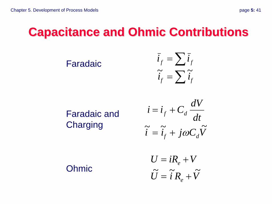
Capacitance and Ohmic ContributionsCapacitance and Ohmic Contributions
∑∑
=
=
ff
ff
ii
ii~~
Faradaic
VCjiidtdVCii
df
df
~~~ ω+=
+=Faradaic and Charging
VRiU
ViRU
e
e~~~ +=
+=Ohmic
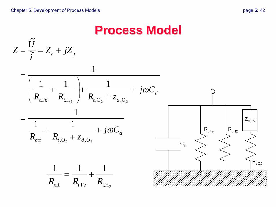
Chapter 5. Development of Process Models page 5: 42
ddt
ddtt,t,
jr
CjzRR
CjzRRR
jZZiUZ
ω
ω
++
+=
++
+⎟⎟⎠
⎞⎜⎜⎝
⎛+
=
+==
22
222
O,O,eff
O,O,HFe
111
1111
~~
2eff Fe H
1 1 1
t, t,R R R= +
Process ModelProcess Model
Rt,O2
Rt,H2Rt,Fe
Cdl
Zd,O2
Chapter 5. Development of Process Models page 5: 43
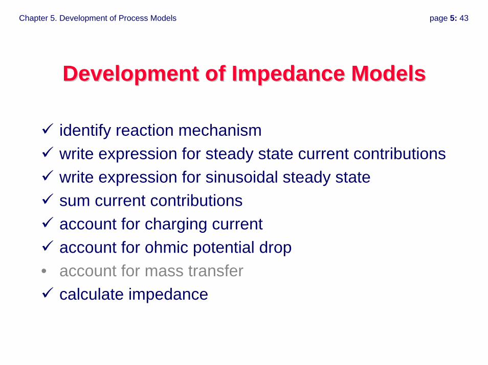
Development of Impedance ModelsDevelopment of Impedance Models
identify reaction mechanismwrite expression for steady state current contributionswrite expression for sinusoidal steady statesum current contributionsaccount for charging currentaccount for ohmic potential drop
• account for mass transfercalculate impedance

Chapter 5. Development of Process Models page 5: 44
Mass TransferMass Transfer
Chapter 5. Development of Process Models page 5: 45
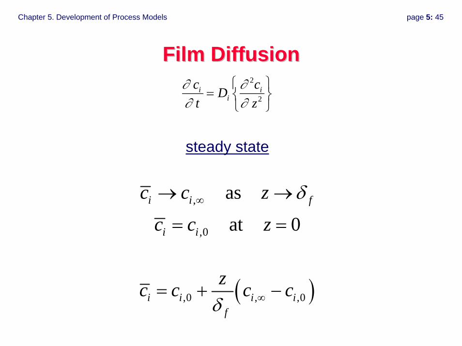
Film DiffusionFilm Diffusion2
2i i
ic cDt z
∂ ∂∂ ∂
⎧ ⎫= ⎨ ⎬
⎩ ⎭
,
,0
as
at 0i i f
i i
c c z
c c z
δ∞→ →
= =
( ),0 , ,0i i i if
zc c c cδ ∞= + −
steady state
Chapter 5. Development of Process Models page 5: 46
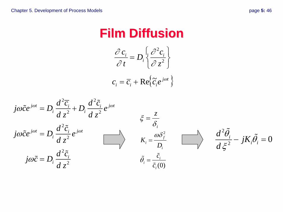
Film DiffusionFilm Diffusion2
2i i
ic cDt z
∂ ∂∂ ∂
⎧ ⎫= ⎨ ⎬
⎩ ⎭
2 2
2 2
2
2
2
2
j t j ti ii i
j t j tii
ii
d c d cj ce D D ed z d zd cj ce D ed zd cj c Dd z
ω ω
ω ω
ω
ω
ω
= +
=
=
{ }tjiii eccc ω~Re+=
2
(0)
fi
i
ii
i
KDc
c
ωδ
θ
=
=
i
zδ
ξ =
2
2 0ii i
d jKdθ
θξ
− =
Chapter 5. Development of Process Models page 5: 47
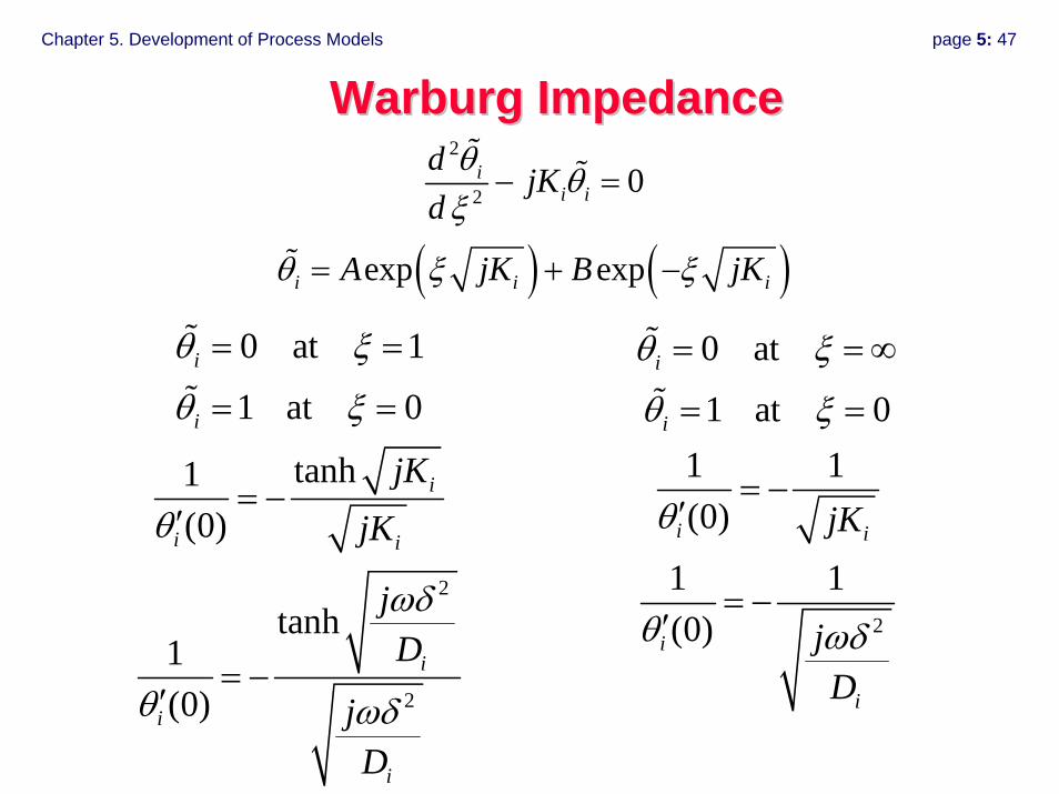
Warburg ImpedanceWarburg Impedance
( ) ( )
2
2 0
exp exp
ii i
i i i
d jKd
A jK B jK
θθ
ξ
θ ξ ξ
− =
= + −
2
2
0 at 1
1 at 0
tanh1(0)
tanh1(0)
i
i
i
i i
i
i
i
jKjK
jD
jD
θ ξ
θ ξ
θ
ωδ
θ ωδ
= =
= =
= −′
= −′
2
0 at
1 at 01 1(0)
1 1(0)
i
i
i i
i
i
jK
jD
θ ξ
θ ξ
θ
θ ωδ
= = ∞
= =
= −′
= −′
Chapter 5. Development of Process Models page 5: 48
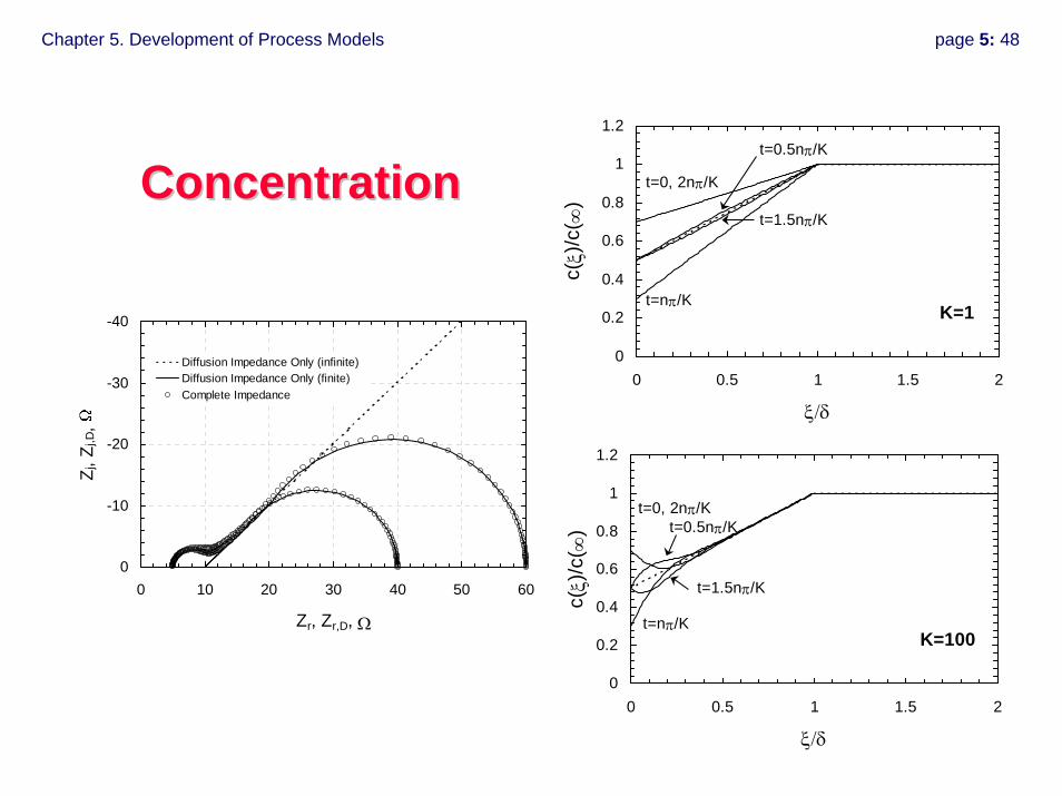
ConcentrationConcentration
0
0.2
0.4
0.6
0.8
1
1.2
0 0.5 1 1.5 2
ξ/δ
c(ξ)
/c( ∞
)
t=0, 2nπ/K
t=nπ/K
t=0.5nπ/K
t=1.5nπ/K
K=100
0
0.2
0.4
0.6
0.8
1
1.2
0 0.5 1 1.5 2
ξ/δ
c(ξ)
/c( ∞
)
t=0, 2nπ/K
t=nπ/K
t=0.5nπ/K
t=1.5nπ/K
K=1-40
-30
-20
-10
00 10 20 30 40 50 60
Zr, Zr,D, Ω
Z j, Z
j,D,
Diffusion Impedance Only (infinite)Diffusion Impedance Only (finite)Complete Impedance
Chapter 5. Development of Process Models page 5: 49
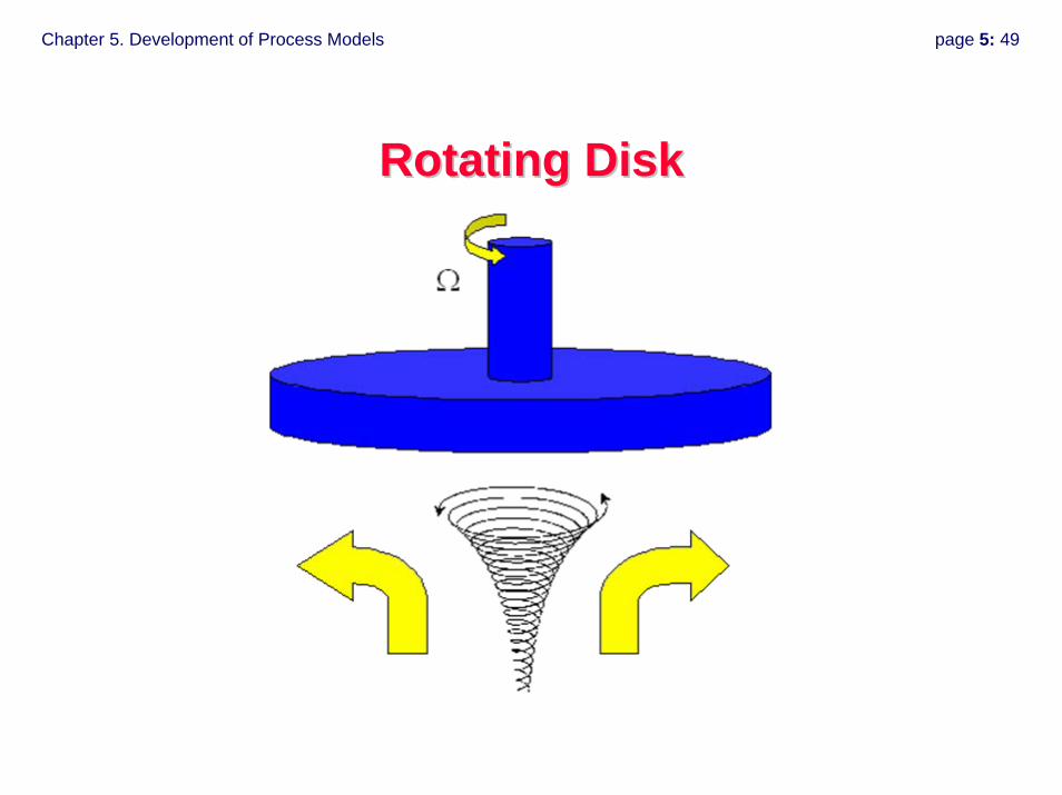
Rotating DiskRotating Disk
Chapter 5. Development of Process Models page 5: 50
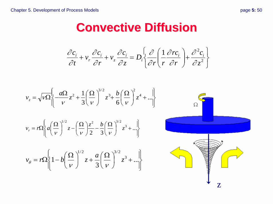
Convective DiffusionConvective Diffusion
⎭⎬⎫
⎩⎨⎧
+⎟⎟⎠
⎞⎜⎜⎝
⎛=++ 2
21zc
rrc
rrD
zcv
rcv
tc ii
ii
zi
ri
∂∂
∂∂
∂∂
∂∂
∂∂
∂∂
⎪⎭
⎪⎬⎫
⎪⎩
⎪⎨⎧
+⎟⎠⎞
⎜⎝⎛ Ω+⎟
⎠⎞
⎜⎝⎛ Ω+
Ω−Ω= ...
631 4
23
2/32 zbzzavz ννν
ν
⎪⎭
⎪⎬⎫
⎪⎩
⎪⎨⎧
+⎟⎠⎞
⎜⎝⎛ Ω−⎟
⎠⎞
⎜⎝⎛ Ω−⎟
⎠⎞
⎜⎝⎛ ΩΩ= ...
323
2/322/1
zbzzarvr ννν
⎪⎭
⎪⎬⎫
⎪⎩
⎪⎨⎧
+⎟⎠⎞
⎜⎝⎛ Ω+⎟
⎠⎞
⎜⎝⎛ Ω−Ω= ...
31 3
2/32/1
zazbrvννθ
z
Chapter 5. Development of Process Models page 5: 51
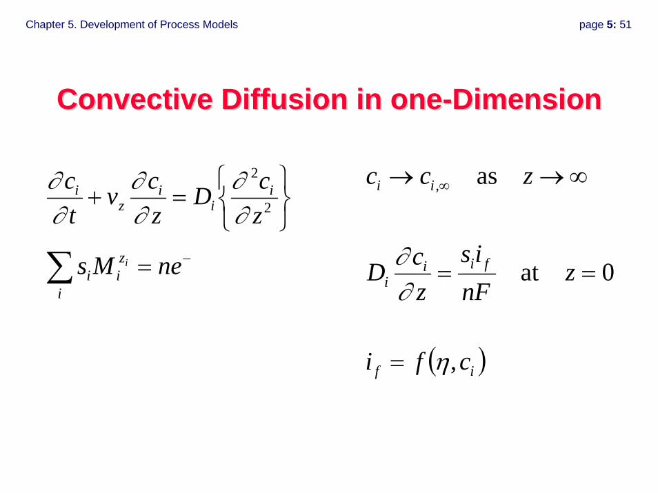
Convective Diffusion in oneConvective Diffusion in one--DimensionDimension
⎭⎬⎫
⎩⎨⎧
=+ 2
2
zcD
zcv
tc i
ii
zi
∂∂
∂∂
∂∂
−=∑ neMsi
zii
i
∞→→ ∞ zcc ii as,
0at == znFis
zcD fii
i ∂∂
( )if cfi ,η=
Chapter 5. Development of Process Models page 5: 52
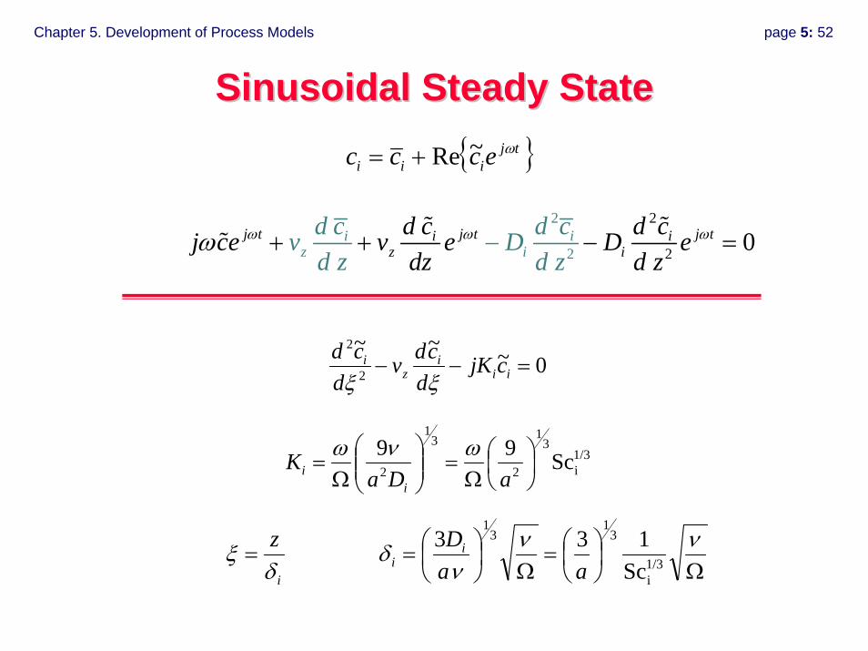
2
2
2
2 0j t j t j ti ii iz iz id c d cv Dd z d
d c d cj ce v e D edz d zz
ω ω ωω + + −− =
Sinusoidal Steady StateSinusoidal Steady State{ }tj
iii eccc ω~Re+=
1/3i
31
2
31
2 Sc99⎟⎠⎞
⎜⎝⎛
Ω=⎟⎟
⎠
⎞⎜⎜⎝
⎛Ω
=aDa
Ki
iωνω
i
zδ
ξ =Ω
⎟⎠⎞
⎜⎝⎛=
Ω⎟⎠⎞
⎜⎝⎛=
ννν
δ 1/3i
31
31
Sc133
aaDi
i
0~~~2
2
=−− iii
zi cjK
dcdv
dcd
ξξ
Chapter 5. Development of Process Models page 5: 53
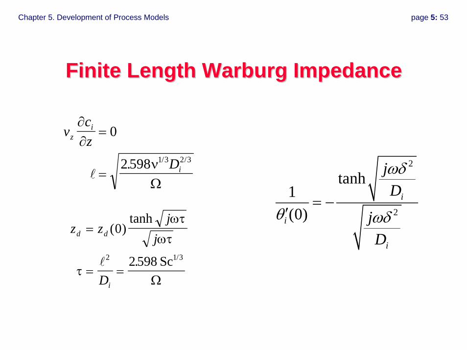
Finite Length Warburg ImpedanceFinite Length Warburg Impedance
vcz
D
zi
i
∂∂
ν
=
=
0
2598 1 3 2 3. / /
Ω
z zj
j
D
d d
i
=
= =
( )tanh
. /
0
25982 1 3
ωτωτ
τSc
Ω
2
2
tanh1(0)
i
i
i
jD
jD
ωδ
θ ωδ= −
′
Chapter 5. Development of Process Models page 5: 54
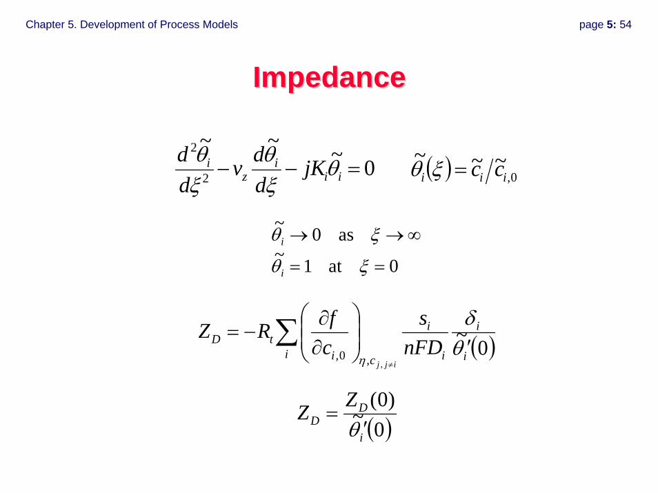
ImpedanceImpedance
0~~~2
2
=−− iii
zi jK
ddv
dd θ
ξθ
ξθ ( ) 0,
~~~iii cc=ξθ
0at1~as0~
==
∞→→
ξθ
ξθ
i
i
( )0~,,0, i
i
i
i
ci itD nFD
scfRZ
ijjθδ
η′⎟⎟
⎠
⎞⎜⎜⎝
⎛
∂∂
−=≠
∑
( )0~)0(
i
DD
ZZθ ′
=
Chapter 5. Development of Process Models page 5: 55
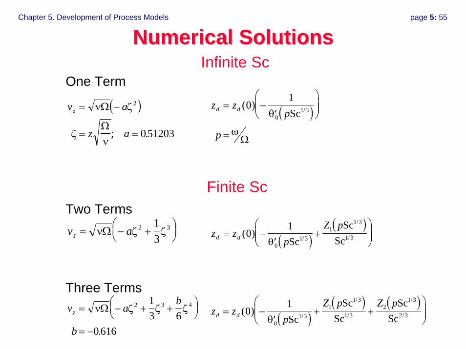
Numerical SolutionsNumerical Solutions
One Term
( )v a
z a
z = −
= =
νΩ ζ
ζν
2
051203Ω
; .
( )z zp
p
d d= −′
⎛
⎝⎜⎜
⎞
⎠⎟⎟
=
( )01
0θ
ω
Sc1/3
Ω
Two Termsv az = − +
⎛⎝⎜
⎞⎠⎟νΩ ζ ζ2 31
3 ( )( )
z zp
Z pd d= −
′+
⎛
⎝⎜⎜
⎞
⎠⎟⎟( )0
1
0
1
θ ScSc
Sc1/3
1/3
1/3
Three Termsv a
b
b
z = − + +⎛⎝⎜
⎞⎠⎟
= −
νΩ ζ ζ ζ2 3 413 6
0 616.( )
( ) ( )z z
pZ p Z p
d d= −′
+ +⎛
⎝⎜⎜
⎞
⎠⎟⎟( )0
1
0
1 2
θ ScSc
ScSc
Sc1/3
1/3
1/3
1/3
2/3
Infinite Sc
Finite Sc

Chapter 5. Development of Process Models page 5: 56
Coupled Diffusion ImpedanceCoupled Diffusion Impedance
, ,, ,
, ,
2, ,
, ,, , ,
i outer i innerd outer d inner
i inner i outerd
i outer i innerinnerd inner d outer
i inner i inner i outer
Dz z
Dz
Dz z j
D D
δδ
δδωδ
+=
⎛ ⎞+⎜ ⎟⎜ ⎟
⎝ ⎠
Chapter 5. Development of Process Models page 5: 57
Interpretation Models for Impedance Interpretation Models for Impedance SpectroscopySpectroscopy
• Models can account rigorously for proposed kinetic and mass transfer mechanisms.
• There are significant differences between models for mass transfer.
• Stochastic errors in impedance spectroscopy are sufficiently small to justify use of accurate models for mass transfer.

Chapter 5. Development of Process Models page 5: 58
Chapter 6. Regression Analysis page 6: 1
Electrochemical Impedance Electrochemical Impedance SpectroscopySpectroscopy
Chapter 6. Regression AnalysisChapter 6. Regression Analysis
• Regression response surfaces– noise– incomplete frequency range
• Adequacy of fit– quantitative– qualitative
© Mark E. Orazem, 2000-2008. All rights reserved.
Chapter 6. Regression Analysis page 6: 2
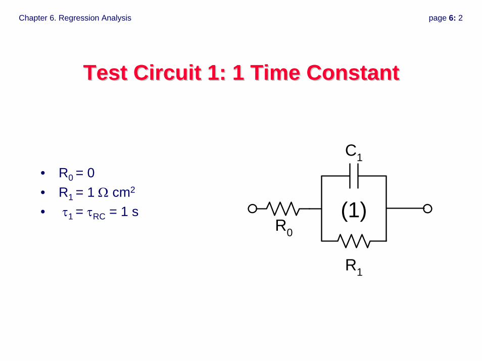
Test Circuit 1: 1 Time ConstantTest Circuit 1: 1 Time Constant
• R0 = 0• R1 = 1 Ω cm2
• τ1 = τRC = 1 sR0
R1
C1
(1)
Chapter 6. Regression Analysis page 6: 3
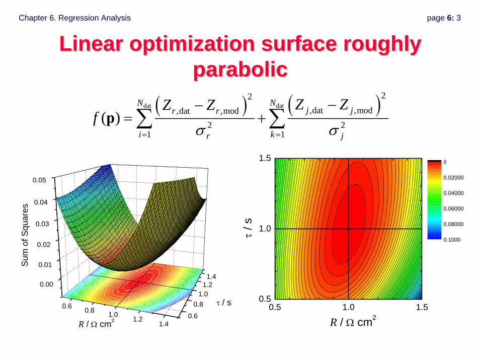
Linear optimization surface roughly Linear optimization surface roughly parabolicparabolic
0.6 0.8 1.01.2
1.4
0.00
0.01
0.02
0.03
0.04
0.05
0.6
0.81.0
1.21.4
Sum
of S
quar
es
τ / s
R / Ω cm2
0.5 1.0 1.50.5
1.0
1.5
R / Ω cm2
τ / s
0
0.02000
0.04000
0.06000
0.08000
0.1000
( ) ( )dat dat22
,dat ,mod,dat ,mod2 2
1 1( )
N Nj jr r
i kr j
Z ZZ Zf
σ σ= =
−−= +∑ ∑p
Chapter 6. Regression Analysis page 6: 4
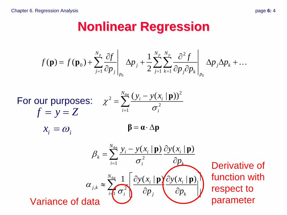
Nonlinear RegressionNonlinear Regression
0 0
2
01 1 1
1( ) ( )2
p p pN N N
j j kj j kj j kp p
f ff f p p pp p p= = =
∂ ∂= + Δ + Δ Δ +
∂ ∂ ∂∑ ∑∑p p …
= ⋅ Δβ α p
dat
21
( | ) ( | )Ni i i
ki i k
y y x y xp
βσ=
− ∂=
∂∑ p p
dat
, 21
1 ( | ) ( | )Ni i
j ki i j k
y x y xp p
ασ=
⎡ ⎤∂ ∂≈ ⎢ ⎥
∂ ∂⎢ ⎥⎣ ⎦∑ p p
dat 22
21
( ( | ))Ni i
i i
y y xχσ=
−= ∑ p
i i
f y Zx ω= =
=
For our purposes:
Variance of data
Derivative of function with respect to parameter
Chapter 6. Regression Analysis page 6: 5
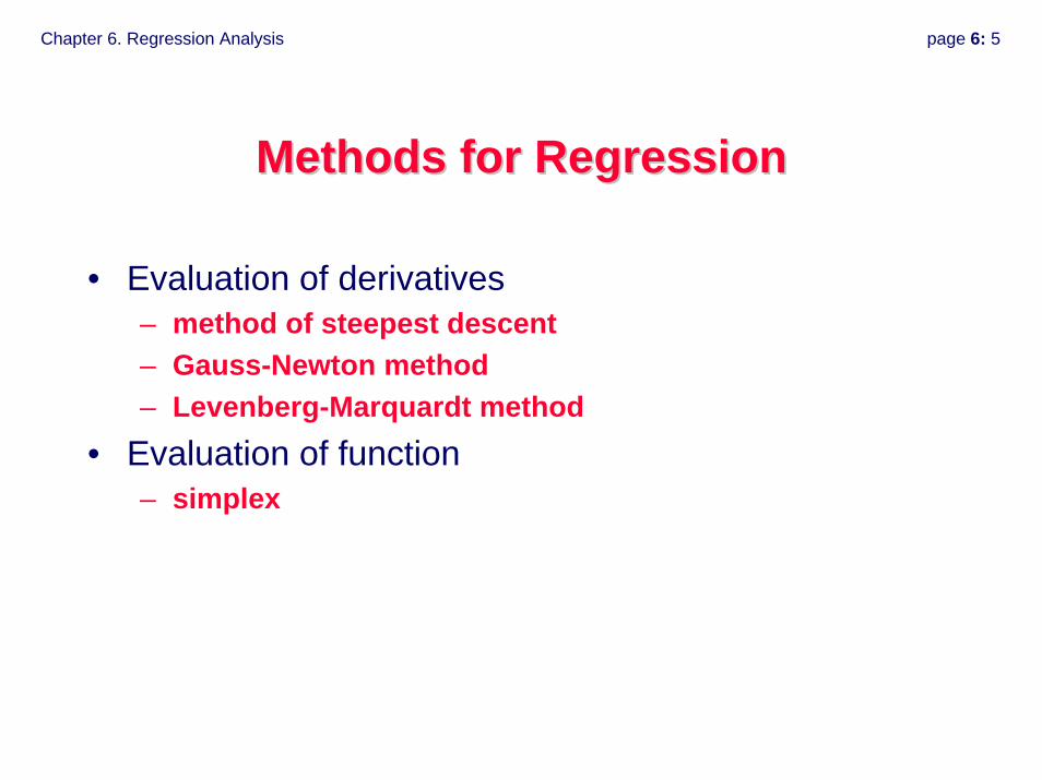
Methods for RegressionMethods for Regression
• Evaluation of derivatives– method of steepest descent– Gauss-Newton method– Levenberg-Marquardt method
• Evaluation of function– simplex
Chapter 6. Regression Analysis page 6: 6
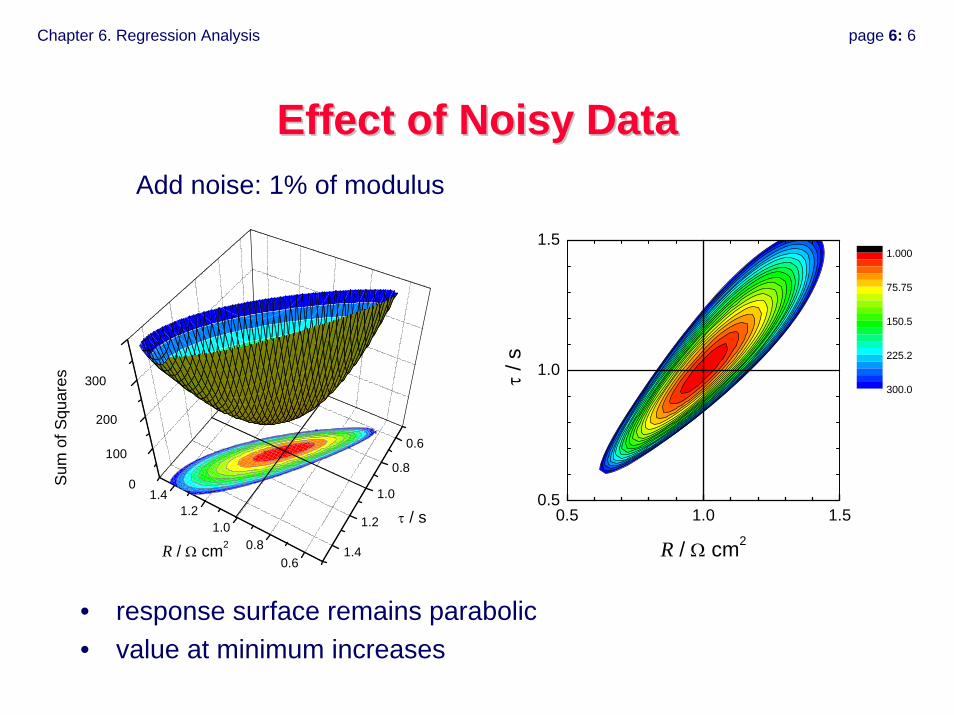
Effect of Noisy DataEffect of Noisy Data
0.5 1.0 1.50.5
1.0
1.5
R / Ω cm2
τ / s
1.000
75.75
150.5
225.2
300.0
• response surface remains parabolic• value at minimum increases
0.6
0.8
1.0
1.2
1.40.6
0.81.0
1.21.4
0
100
200
300
Sum
of S
quar
es
R / Ω cm2
τ / s
Add noise: 1% of modulus
Chapter 6. Regression Analysis page 6: 7
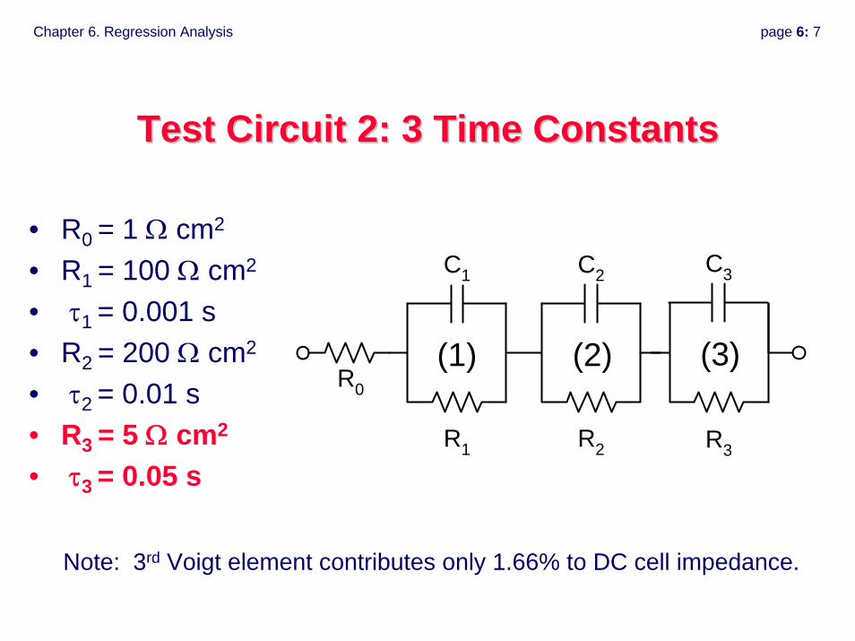
Test Circuit 2: 3 Time ConstantsTest Circuit 2: 3 Time Constants
R0
R1
C1
(1)
R2
C2
(2)
R3
C3
(3)
• R0 = 1 Ω cm2
• R1 = 100 Ω cm2
• τ1 = 0.001 s• R2 = 200 Ω cm2
• τ2 = 0.01 s• R3 = 5 Ω cm2
• τ3 = 0.05 s
Note: 3rd Voigt element contributes only 1.66% to DC cell impedance.
Chapter 6. Regression Analysis page 6: 8
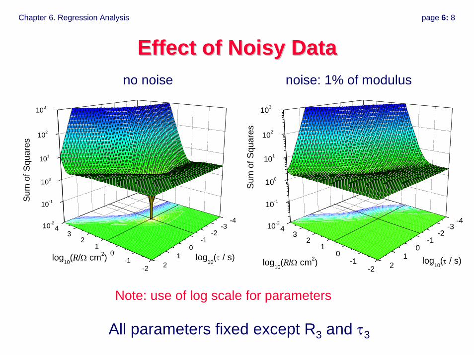
Effect of Noisy DataEffect of Noisy Data
All parameters fixed except R3 and τ3
-4-3
-2-1
01
2-2-1
01
23
410-2
10-1
100
101
102
103
Sum
of S
quar
es log10(R/Ω cm2) log10(τ / s)
noise: 1% of modulus
-4-3
-2-1
01
2-2-1
01
23
410-2
10-1
100
101
102
103
Sum
of S
quar
es
log10(R/Ω cm2) log10(τ / s)
no noise
Note: use of log scale for parameters
Chapter 6. Regression Analysis page 6: 9
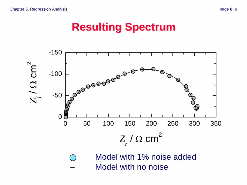
Resulting SpectrumResulting Spectrum
0 50 100 150 200 250 300 3500
-50
-100
-150
Z j /
Ω c
m2
Zr / Ω cm2
Model with 1% noise added− Model with no noise
Chapter 6. Regression Analysis page 6: 10
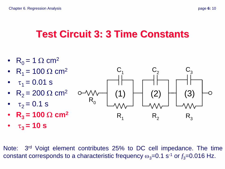
Test Circuit 3: 3 Time ConstantsTest Circuit 3: 3 Time Constants
R0
R1
C1
(1)
R2
C2
(2)
R3
C3
(3)
• R0 = 1 Ω cm2
• R1 = 100 Ω cm2
• τ1 = 0.01 s• R2 = 200 Ω cm2
• τ2 = 0.1 s• R3 = 100 Ω cm2
• τ3 = 10 s
Note: 3rd Voigt element contributes 25% to DC cell impedance. The time constant corresponds to a characteristic frequency ω3=0.1 s-1 or f3=0.016 Hz.
Chapter 6. Regression Analysis page 6: 11
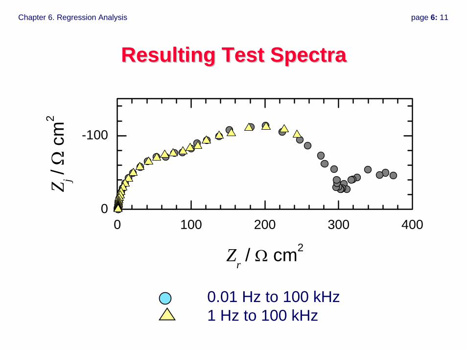
Resulting Test SpectraResulting Test Spectra
0 100 200 300 4000
-100
Z j / Ω
cm
2
Zr / Ω cm2
0.01 Hz to 100 kHz1 Hz to 100 kHz
Chapter 6. Regression Analysis page 6: 12
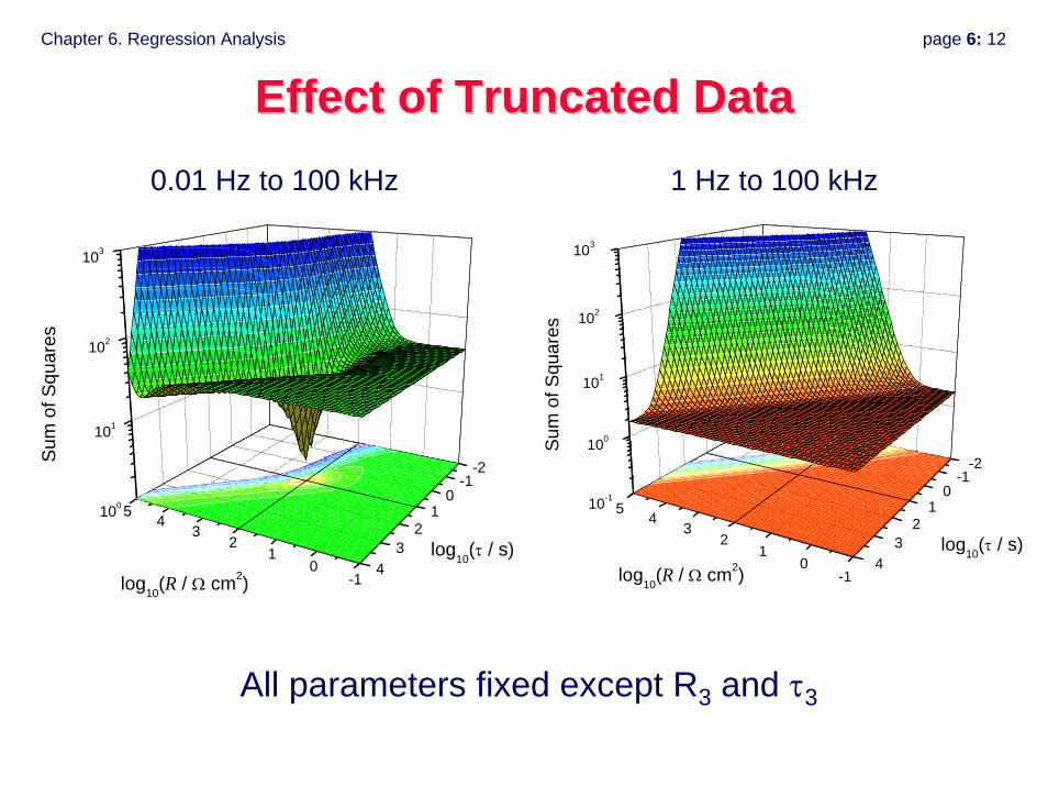
Effect of Truncated DataEffect of Truncated Data
All parameters fixed except R3 and τ3
-2-1
01
23
4-1
01
23
45100
101
102
103
Sum
of S
quar
es
log10(R / Ω cm2)
log10(τ / s)
0.01 Hz to 100 kHz
-2-1
01
23
4-1
01
23
4510-1
100
101
102
103
Sum
of S
quar
es log10(R / Ω cm2)
log10(τ / s)
1 Hz to 100 kHz
Chapter 6. Regression Analysis page 6: 13
Conclusions from Test Spectra Conclusions from Test Spectra
• The presence of noise in data can have a direct impact on model identification and on the confidence interval for the regressed parameters.
• The correctness of the model does not determine the number of parameters that can be obtained.
• The frequency range of the data can have a direct impact on model identification.
• The model identification problem is intricately linked to the error identification problem. In other words, analysis of data requires analysis of the error structure of the measurement.

Chapter 6. Regression Analysis page 6: 14
When Is the Fit Adequate?When Is the Fit Adequate?
• Chi-squared statistic– includes variance of data– should be near the degree of freedom
• Visual examination– should look good– some plots show better sensitivity than others
• Parameter confidence intervals– based on linearization about solution– should not include zero
Chapter 6. Regression Analysis page 6: 15
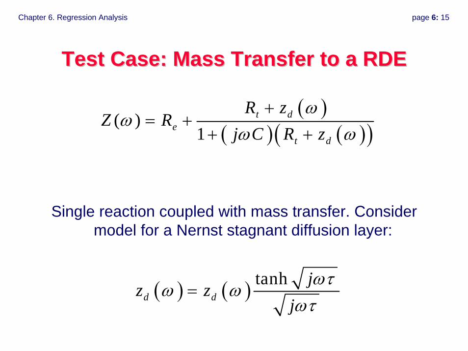
Test Case: Mass Transfer to a RDETest Case: Mass Transfer to a RDE
Single reaction coupled with mass transfer. Consider model for a Nernst stagnant diffusion layer:
( )( ) ( )( )
( )1
t de
t d
R zZ R
j C R zω
ωω ω
+= +
+ +
( ) ( ) tanhd d
jz z
jωτ
ω ωωτ
=
Chapter 6. Regression Analysis page 6: 16
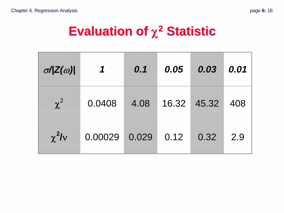
Evaluation of Evaluation of χχ22 StatisticStatistic
σ/|Z(ω)| 1 0.1 0.05 0.03 0.01
χ2 0.0408 4.08 16.32 45.32 408
χ2/ν 0.00029 0.029 0.12 0.32 2.9
Chapter 6. Regression Analysis page 6: 17
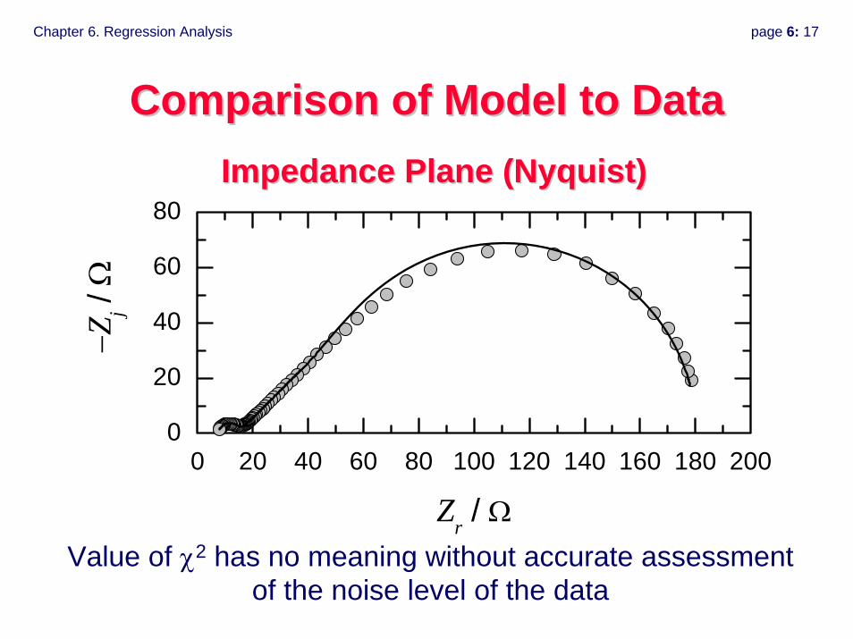
Comparison of Model to DataComparison of Model to Data
0 20 40 60 80 100 120 140 160 180 2000
20
40
60
80
−Zj /
Ω
Zr / Ω
Impedance Plane (Impedance Plane (NyquistNyquist))
Value of χ2 has no meaning without accurate assessment of the noise level of the data

Chapter 6. Regression Analysis page 6: 18
ModulusModulus
10-2 10-1 100 101 102 103 104
10
100
|Z| /
Ω
f / Hz
Chapter 6. Regression Analysis page 6: 19
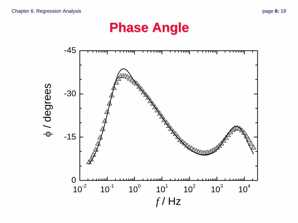
Phase AnglePhase Angle
10-2 10-1 100 101 102 103 1040
-15
-30
-45
φ
/ deg
rees
f / Hz
Chapter 6. Regression Analysis page 6: 20
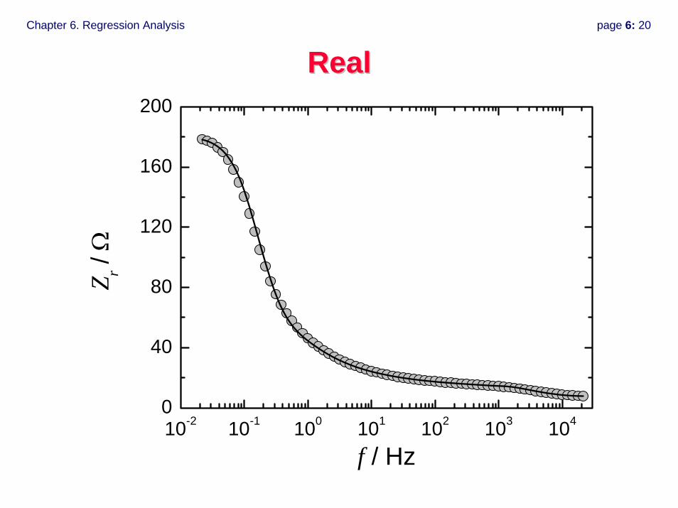
RealReal
10-2 10-1 100 101 102 103 1040
40
80
120
160
200
Z r /
Ω
f / Hz
Chapter 6. Regression Analysis page 6: 21
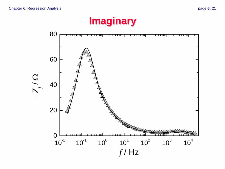
ImaginaryImaginary
10-2 10-1 100 101 102 103 1040
20
40
60
80
−Zj /
Ω
f / Hz
Chapter 6. Regression Analysis page 6: 22
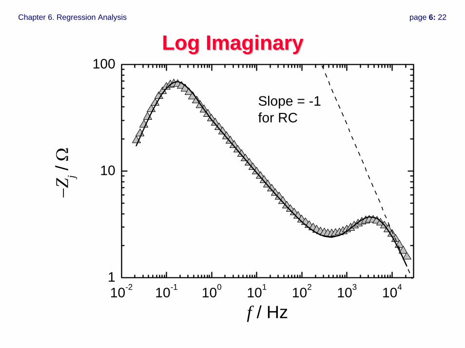
Log ImaginaryLog Imaginary
10-2 10-1 100 101 102 103 1041
10
100
Slope = -1 for RC
−Z
j / Ω
f / Hz
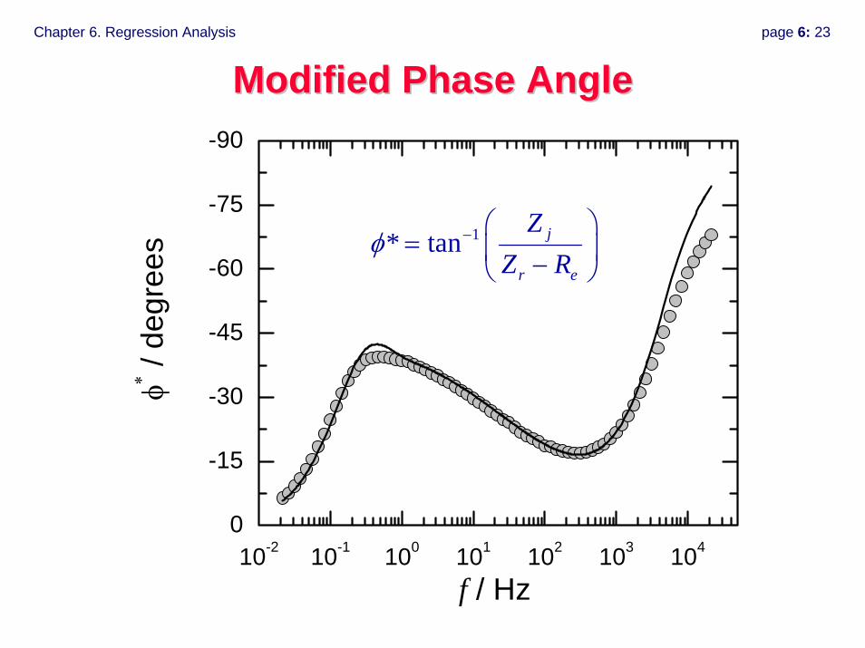
Chapter 6. Regression Analysis page 6: 23
Modified Phase AngleModified Phase Angle
10-2 10-1 100 101 102 103 1040
-15
-30
-45
-60
-75
-90φ∗ /
degr
ees
f / Hz
1* tan j
r e
ZZ R
φ − ⎛ ⎞= ⎜ ⎟−⎝ ⎠
Chapter 6. Regression Analysis page 6: 24
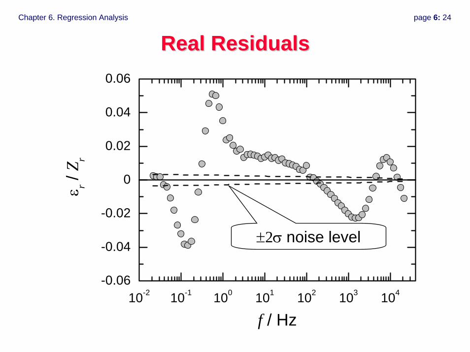
Real ResidualsReal Residuals
10-2 10-1 100 101 102 103 104-0.06
-0.04
-0.02
0
0.02
0.04
0.06
ε r /
Z r
f / Hz
±2σ noise level
Chapter 6. Regression Analysis page 6: 25
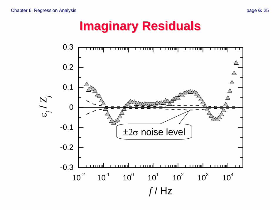
Imaginary ResidualsImaginary Residuals
10-2 10-1 100 101 102 103 104-0.3
-0.2
-0.1
0
0.1
0.2
0.3ε j /
Z j
f / Hz
±2σ noise level
Chapter 6. Regression Analysis page 6: 26
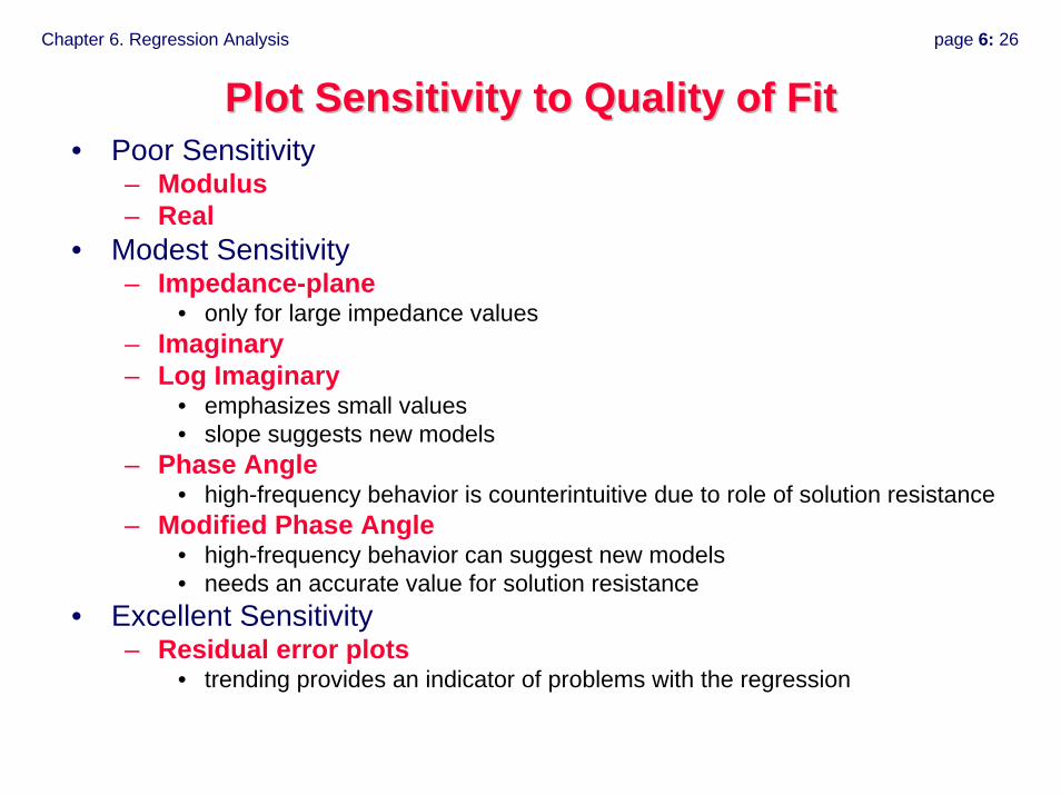
Plot Sensitivity to Quality of FitPlot Sensitivity to Quality of Fit• Poor Sensitivity
– Modulus– Real
• Modest Sensitivity– Impedance-plane
• only for large impedance values– Imaginary– Log Imaginary
• emphasizes small values• slope suggests new models
– Phase Angle• high-frequency behavior is counterintuitive due to role of solution resistance
– Modified Phase Angle• high-frequency behavior can suggest new models• needs an accurate value for solution resistance
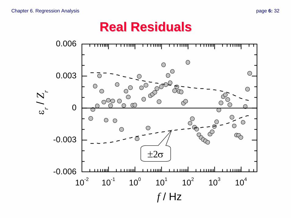
• Excellent Sensitivity– Residual error plots
• trending provides an indicator of problems with the regression
Chapter 6. Regression Analysis page 6: 27
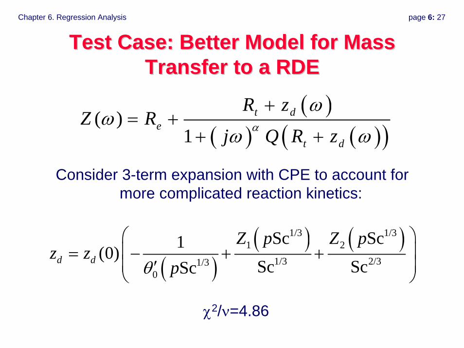
Test Case: Better Model for Mass Test Case: Better Model for Mass Transfer to a RDETransfer to a RDE
( )( ) ( )( )
( )1
t de
t d
R zZ R
j Q R zα
ωω
ω ω
+= +
+ +
Consider 3-term expansion with CPE to account for more complicated reaction kinetics:
( )( ) ( )1/3 1/3
1 21/3 2/31/3
0
Sc Sc1(0)Sc ScScd d
Z p Z pz z
pθ
⎛ ⎞⎜ ⎟= − + +⎜ ⎟′⎝ ⎠
χ2/ν=4.86
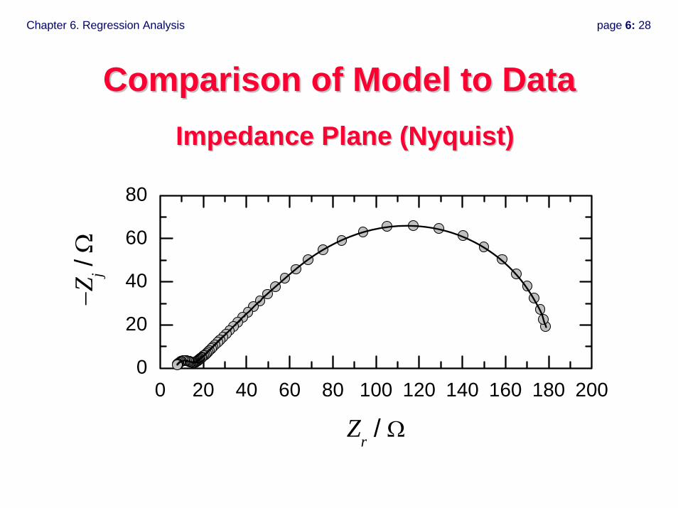
Chapter 6. Regression Analysis page 6: 28
Comparison of Model to DataComparison of Model to DataImpedance Plane (Impedance Plane (NyquistNyquist))
0 20 40 60 80 100 120 140 160 180 2000
20
40
60
80
−Zj /
Ω
Zr / Ω
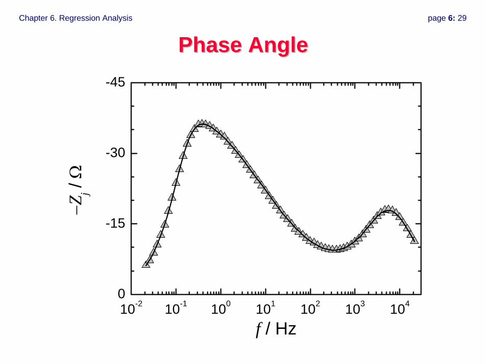
Chapter 6. Regression Analysis page 6: 29
Phase AnglePhase Angle
10-2 10-1 100 101 102 103 1040
-15
-30
-45
−Z
j / Ω
f / Hz
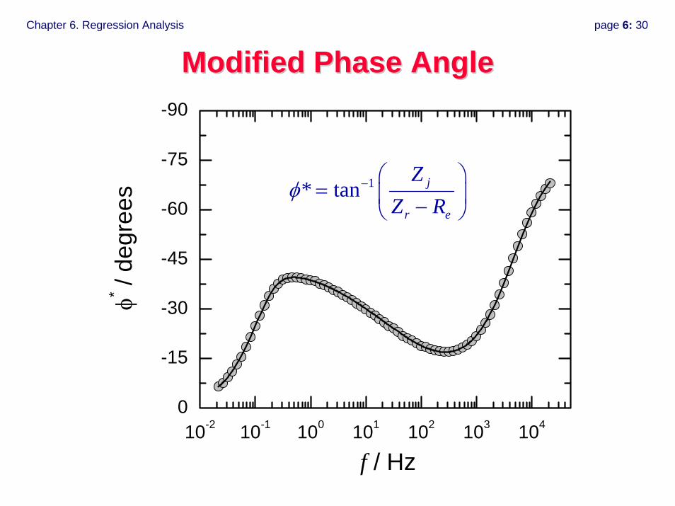
Chapter 6. Regression Analysis page 6: 30
Modified Phase AngleModified Phase Angle
10-2 10-1 100 101 102 103 1040
-15
-30
-45
-60
-75
-90φ* /
degr
ees
f / Hz
1* tan j
r e
ZZ R
φ − ⎛ ⎞= ⎜ ⎟−⎝ ⎠
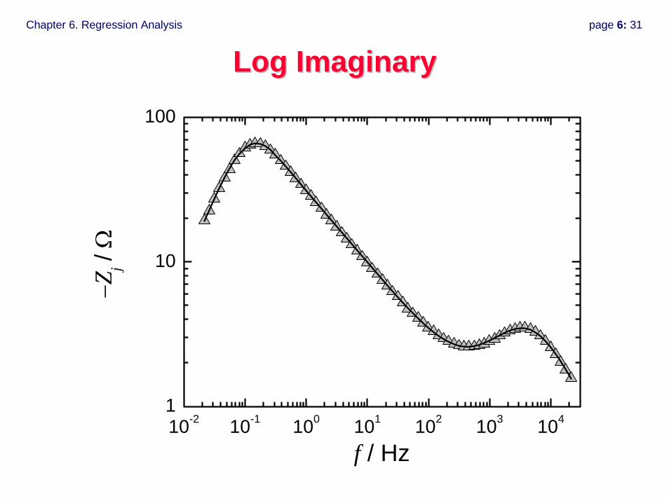
Chapter 6. Regression Analysis page 6: 31
Log ImaginaryLog Imaginary
10-2 10-1 100 101 102 103 1041
10
100
−Z
j / Ω
f / Hz
Chapter 6. Regression Analysis page 6: 32
10-2 10-1 100 101 102 103 104-0.006
-0.003
0
0.003
0.006ε r /
Z r
f / Hz
Real ResidualsReal Residuals
±2σ
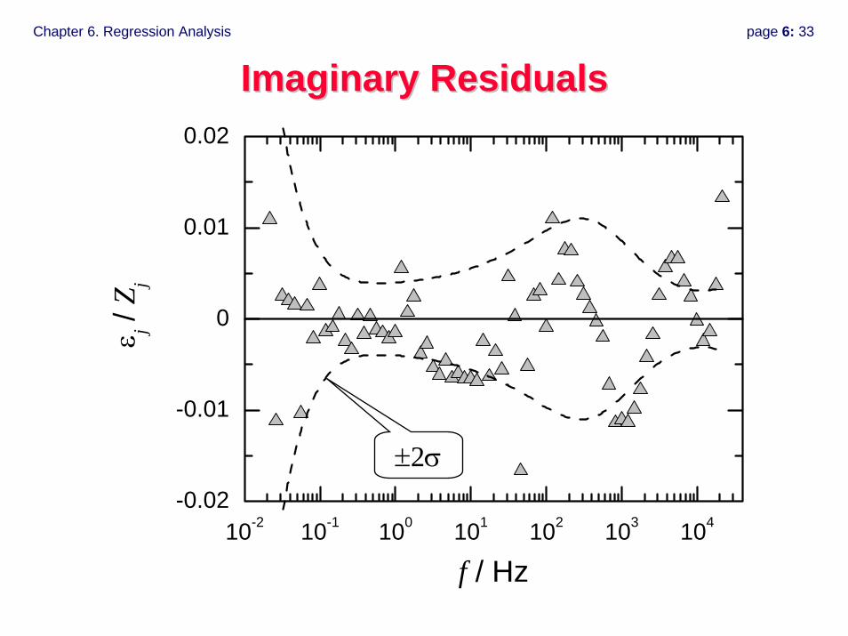
Chapter 6. Regression Analysis page 6: 33
10-2 10-1 100 101 102 103 104-0.02
-0.01
0
0.01
0.02ε j /
Z j
f / Hz
Imaginary ResidualsImaginary Residuals
±2σ
Chapter 6. Regression Analysis page 6: 34
Confidence IntervalsConfidence Intervals
• Based on linearization about trial solution• Assumption valid for good fits
– for normally distributed fitting errors– small estimated standard deviations
• Can use Monte Carlo simulations to test assumptions
Chapter 6. Regression Analysis page 6: 35
Regression of Models to DataRegression of Models to Data
• Regression is strongly influenced by – stochastic errors in data– incomplete frequency range– incorrect or incomplete models
• Some plots more sensitive to fit quality than others.• Quantitative measures of fit quality require
independent assessment of error structure.• The model identification problem is intricately linked
to the error identification problem.

Chapter 6. Regression Analysis page 6: 36
Chapter 7. Error Structure page 7: 1
Electrochemical Impedance Electrochemical Impedance SpectroscopySpectroscopy
Chapter 7. Error StructureChapter 7. Error Structure
• Contributions to error structure• Weighting strategies• General approach for error analysis• Experimental results
© Mark E. Orazem, 2000-2008. All rights reserved.
Chapter 7. Error Structure page 7: 2
Error Analysis Increasingly Important Error Analysis Increasingly Important
• Improved Instrumentation– improved signal-to-noise– more data– more detailed interpretation of data possible
• New experimental techniques– more ways to study a system– proper weight must be assigned to each experiment– error analysis used to improve experimental design
• Improved computational speed– increased use of regression– increased use of detailed models
Chapter 7. Error Structure page 7: 3
Contributions to Error StructureContributions to Error Structure
• Sampling Errors
• Stochastic Phenomena• Bias Errors
– Lack of Fit– Changing baseline (non-stationary processes)– Instrumental artifacts
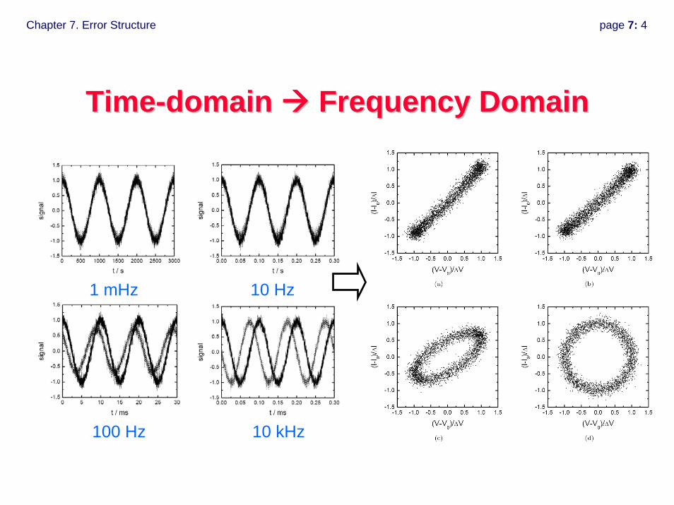
Chapter 7. Error Structure page 7: 4
TimeTime--domain domain Frequency DomainFrequency Domain
1 mHz 10 Hz
100 Hz 10 kHz
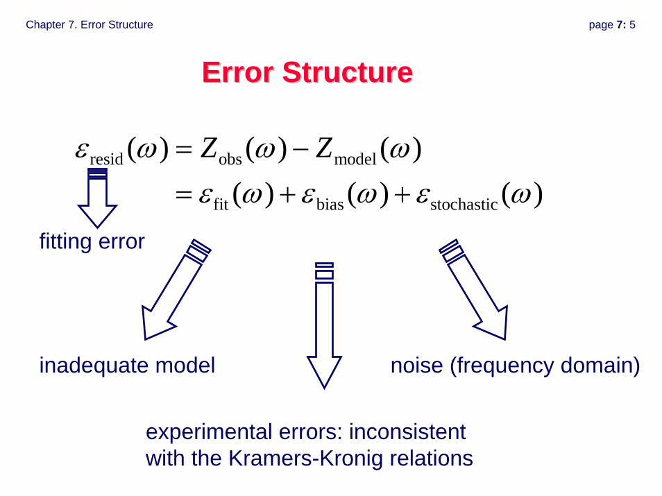
Chapter 7. Error Structure page 7: 5
Error StructureError Structure
resid obs model
fit bias stochastic
( ) ( ) ( )( ) ( ) ( )
Z Zε ω ω ωε ω ε ω ε ω
= −= + +
inadequate model noise (frequency domain)
experimental errors: inconsistent with the Kramers-Kronig relations
fitting error
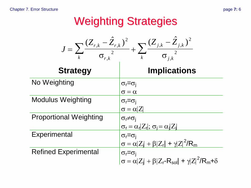
Chapter 7. Error Structure page 7: 6
Weighting StrategiesWeighting Strategies
JZ Z Z Zr k r k
r kk
j k j k
j kk=
−+
−∑ ∑( ) ( ), ,
,
, ,
,
2
2
2
2σ σ
Strategy ImplicationsNo Weighting σr=σj
σ = αModulus Weighting σr=σj
σ = α|Ζ|Proportional Weighting σr≠σj
σr = αr|Ζr|; σj = αj|Ζj|Experimental σr=σj
σ = α|Ζj| + β|Ζr| + γ|Ζ|2/RmRefined Experimental σr=σj
σ = α|Ζj| + β|Ζr-Rsol| + γ|Ζ|2/Rm+δ
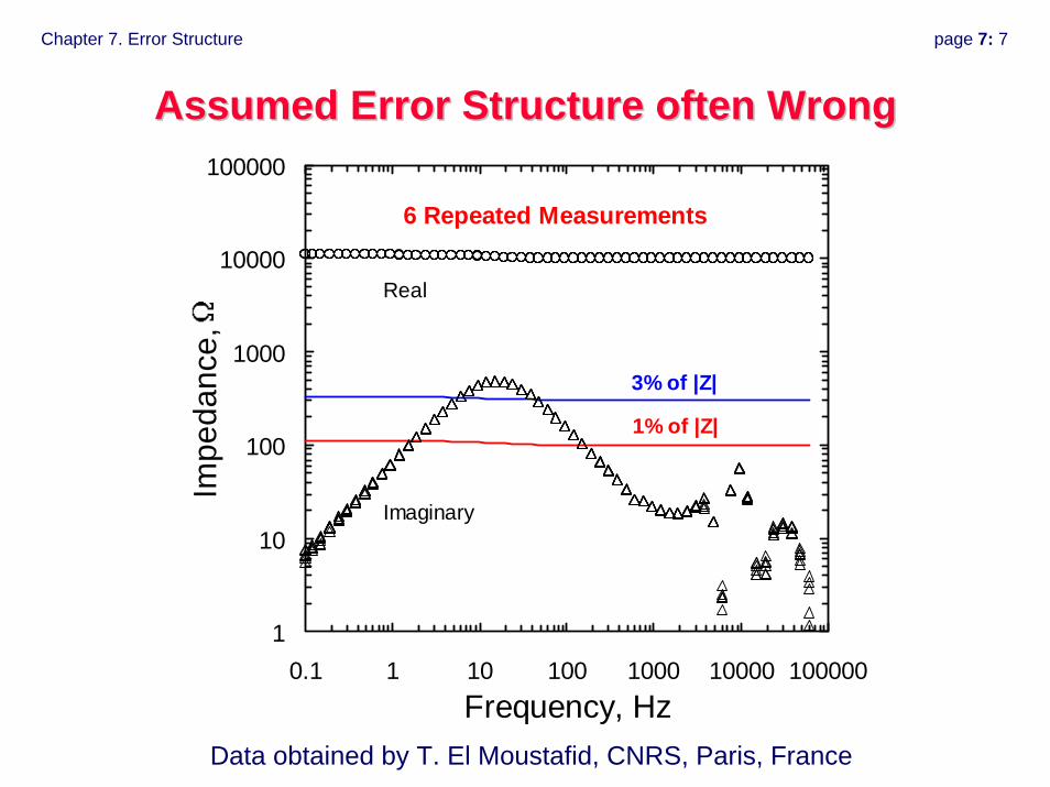
Chapter 7. Error Structure page 7: 7
Assumed Error Structure often WrongAssumed Error Structure often Wrong
1
10
100
1000
10000
100000
0.1 1 10 100 1000 10000 100000Frequency, Hz
Impe
danc
e,
3% of |Z|
1% of |Z|
6 Repeated Measurements
Real
Imaginary
Data obtained by T. El Moustafid, CNRS, Paris, France
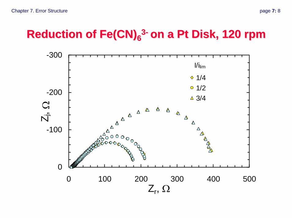
Chapter 7. Error Structure page 7: 8
Reduction of Fe(CN)Reduction of Fe(CN)6633-- on a Pt Disk, 120 rpmon a Pt Disk, 120 rpm
-300
-200
-100
00 100 200 300 400 500
Zr, Ω
Z j, Ω
1/41/23/4
I/ilim
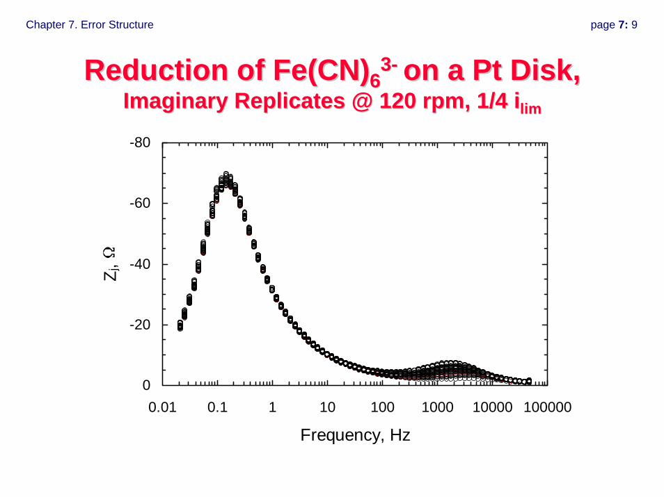
Chapter 7. Error Structure page 7: 9
Reduction of Fe(CN)Reduction of Fe(CN)6633-- on a Pt Disk, on a Pt Disk,
Imaginary Replicates @ 120 rpm, 1/4 Imaginary Replicates @ 120 rpm, 1/4 iilimlim
-80
-60
-40
-20
00.01 0.1 1 10 100 1000 10000 100000
Frequency, Hz
Z j,
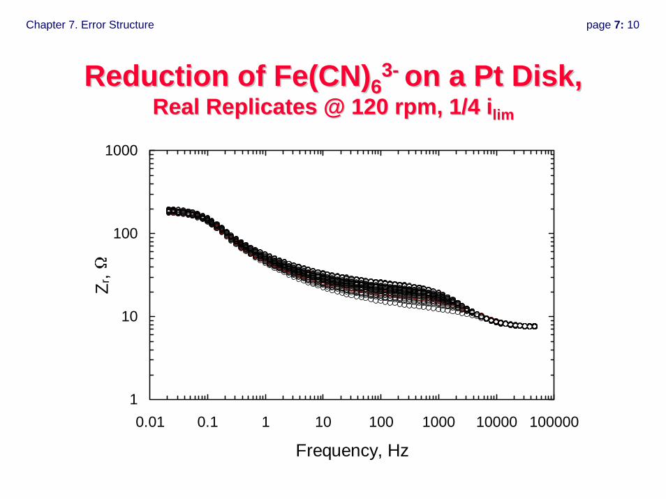
Chapter 7. Error Structure page 7: 10
Reduction of Fe(CN)Reduction of Fe(CN)6633-- on a Pt Disk, on a Pt Disk,
Real Replicates @ 120 rpm, 1/4 Real Replicates @ 120 rpm, 1/4 iilimlim
1
10
100
1000
0.01 0.1 1 10 100 1000 10000 100000
Frequency, Hz
Z r,
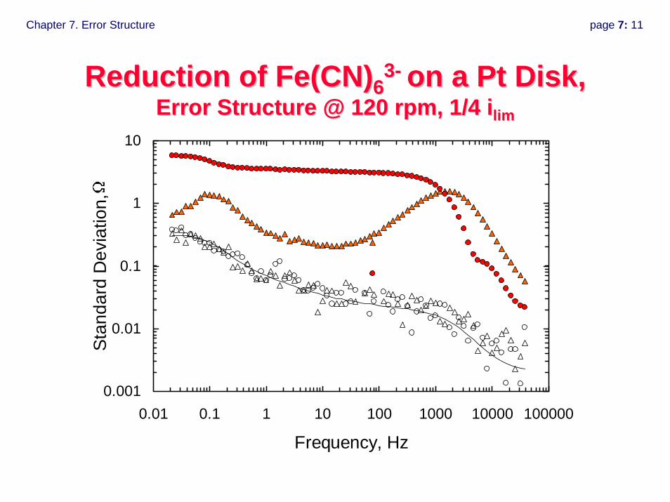
Chapter 7. Error Structure page 7: 11
Reduction of Fe(CN)Reduction of Fe(CN)6633-- on a Pt Disk, on a Pt Disk,
Error Structure @ 120 rpm, 1/4 Error Structure @ 120 rpm, 1/4 iilimlim
0.001
0.01
0.1
1
10
0.01 0.1 1 10 100 1000 10000 100000
Frequency, Hz
Stan
dard
Dev
iatio
n,
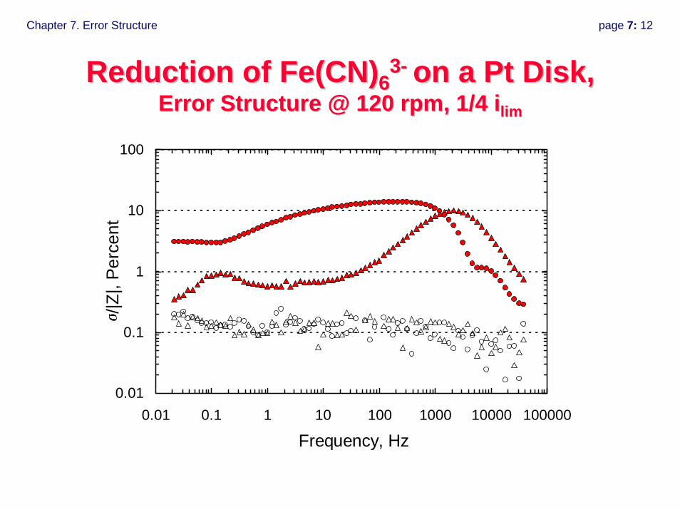
Chapter 7. Error Structure page 7: 12
Reduction of Fe(CN)Reduction of Fe(CN)6633-- on a Pt Disk, on a Pt Disk,
Error Structure @ 120 rpm, 1/4 Error Structure @ 120 rpm, 1/4 iilimlim
0.01
0.1
1
10
100
0.01 0.1 1 10 100 1000 10000 100000
Frequency, Hz
/|Z|,
Perc
ent
Chapter 7. Error Structure page 7: 13
Interpretation of Impedance SpectraInterpretation of Impedance Spectra• Need physical insight and knowledge of error structure
– stochastic component• weighting• determination of model adequacy• experimental design
– bias component• suitable frequency range• experimental design
• Approach is general– electrochemical impedance spectroscopies– optical spectroscopies– mechanical spectroscopies

Chapter 7. Error Structure page 7: 14
Chapter 8. Kramers-Kronig Relations page 8: 1
Electrochemical Impedance Electrochemical Impedance SpectroscopySpectroscopy
Chapter 8. KramersChapter 8. Kramers--Kronig RelationsKronig Relations
• Mathematical form and interpretation• Application to noisy data• Methods to evaluate consistency
© Mark E. Orazem, 2000-2008. All rights reserved.
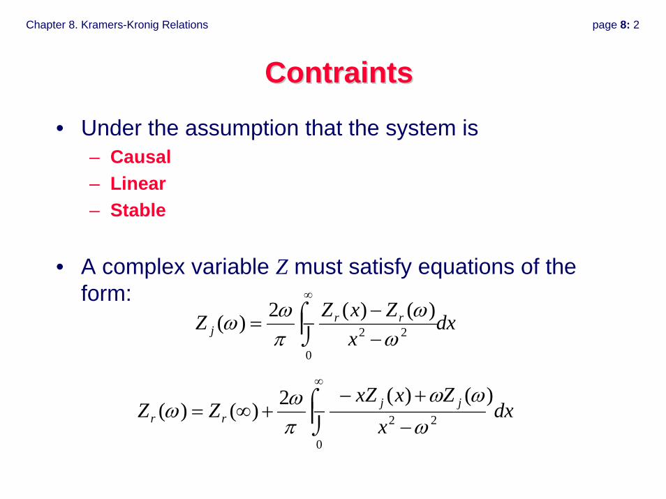
Chapter 8. Kramers-Kronig Relations page 8: 2
ContraintsContraints
• Under the assumption that the system is– Causal– Linear– Stable
• A complex variable Z must satisfy equations of the form:
dxx
ZxZZ rrj ⎮⌡
⌠−−
−=∞
0
22)()(2)(
ωω
πωω
dxx
ZxxZZZ jj
rr ⎮⌡⌠
−
+−−+∞=
∞
0
22
)()(2)()(ω
ωωπωω
Chapter 8. Kramers-Kronig Relations page 8: 3
Use of KramersUse of Kramers--Kronig RelationsKronig Relations
• Concept– if data do not satisfy Kramers-Kronig relations, a
condition of the derivation must not be satisfied• stationarity / causality• linearity• stability
– interpret result in terms of • instrument artifact• changing baseline
– if data satisfy Kramers-Kronig relations, conditions of the derivation may be satisfied
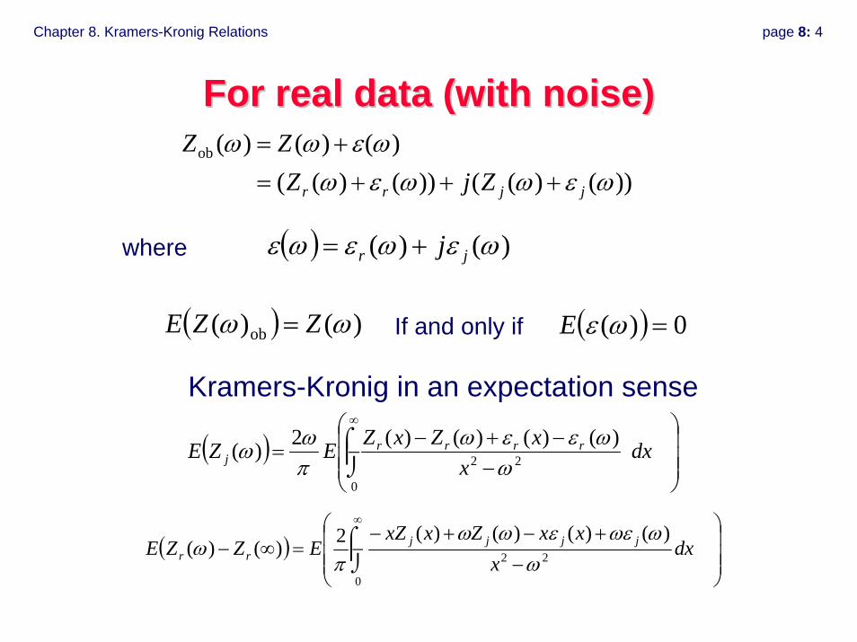
Chapter 8. Kramers-Kronig Relations page 8: 4
For real data (with noise)For real data (with noise)
))()(())()(()()()(ob
ωεωωεωωεωω
jjrr ZjZZZ
+++=+=
( ) )()( ωεωεωε jr j+=
( ) )()( ob ωω ZZE = ( ) 0)( =ωεE
where
If and only if
( )⎟⎟⎟
⎠
⎞
⎜⎜⎜
⎝
⎛⎮⌡⌠
−−+−
−=
∞
0
22)()()()(2)( dx
xxZxZEZE rrrr
j ωωεεω
πωω
( )⎟⎟⎟
⎠
⎞
⎜⎜⎜
⎝
⎛⎮⌡⌠
−
+−+−−=∞−
∞
0
22
)()()()(2)()( dxx
xxZxxZEZZE jjjj
rr ωωωεεωω
πω
Kramers-Kronig in an expectation sense

Chapter 8. Kramers-Kronig Relations page 8: 5
The KramersThe Kramers--Kronig relations can be Kronig relations can be satisfied ifsatisfied if
• This means– the process must be stationary in the sense of replication at every
measurement frequency. – As the impedance is sampled at a finite number of frequencies, εr(x)
represents the error between an interpolated function and the “true”impedance value at frequency x. In the limit that quadrature and interpolation errors are negligible, the residual errors εr(x) should be of the same magnitude as the stochastic noise εr(ω).
0)(2
0
22 =⎟⎟⎟
⎠
⎞
⎜⎜⎜
⎝
⎛⎮⌡⌠
−−∞
dxx
xE r
ωε
πω( ) 0)( =ωεE and
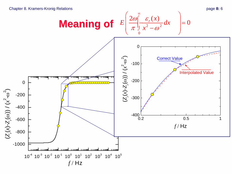
Chapter 8. Kramers-Kronig Relations page 8: 6
10-4 10-3 10-2 10-1 100 101 102 103 104 105
-1000
-800
-600
-400
-200
0
(Zr(x
)-Zr(ω
)) /
(x2 -ω
2 )
f / Hz
Meaning ofMeaning of 2 2
0
2 ( ) 0r xE dxx
ω επ ω
∞⌠⎮⎮⌡
⎛ ⎞⎜ ⎟− =
−⎜ ⎟⎝ ⎠
0.2 0.5 1-400
-300
-200
-100
0
Interpolated Value
Correct Value
(Zr(x
)-Zr(ω
)) /
(x2 -ω
2 )
f / Hz
Chapter 8. Kramers-Kronig Relations page 8: 7
Use of KramersUse of Kramers--Kronig RelationsKronig Relations
• Quadrature errors– require interpolation function
• Missing data at low and high frequency
Chapter 8. Kramers-Kronig Relations page 8: 8
Methods to Resolve Problems of Insufficient Methods to Resolve Problems of Insufficient Frequency RangeFrequency Range
• Direct Integration– Extrapolation
• single RC• polynomials• 1/ω and ω asymptotic behavior
– simultaneous solution for missing data• Regression
– proposed process model– generalized measurement model

Chapter 8. Kramers-Kronig Relations page 8: 9
Chapter 9. Use of Measurement Models page 9: 1
Electrochemical Impedance Electrochemical Impedance SpectroscopySpectroscopy
Chapter 9. Use of Measurement ModelsChapter 9. Use of Measurement Models
• Generalized model• Identification of stochastic component of error structure• Identification of bias component of error structure
© Mark E. Orazem, 2000-2008. All rights reserved.
Chapter 9. Use of Measurement Models page 9: 2
ApproachApproach• Experimental design
– quality (signal-to-noise, bias errors)– information content
• Process model– account for known phenomena– extract information concerning other phenomena
• Regression– uncorrupted frequency range– weighting strategy
• Error analysis - measurement model– stochastic errors– bias errors
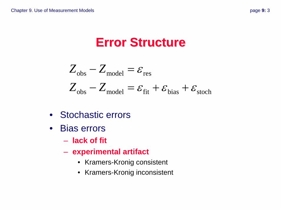
Chapter 9. Use of Measurement Models page 9: 3
Error StructureError Structure
obs model res
obs model fit bias stoch
Z ZZ Z
εε ε ε
− =− = + +
• Stochastic errors• Bias errors
– lack of fit– experimental artifact
• Kramers-Kronig consistent• Kramers-Kronig inconsistent

Chapter 9. Use of Measurement Models page 9: 4
Measurement ModelMeasurement Model
• Superposition of lineshapes
01 1
nk
k k k
RZ Rj R Cω=
= ++∑
Chapter 9. Use of Measurement Models page 9: 5
Identification of Stochastic Component Identification of Stochastic Component of Error Structureof Error Structure
How?• Replicate impedance scans.• Fit measurement model to
each scan:– use modulus or no-
weighting options.– same number of
lineshapes.– parameter estimates do
not include zero.• Calculate standard deviation
of residual errors.• Fit model for error structure.
Why?• Weight regression.• Identify good fit.• Improve experimental
design.
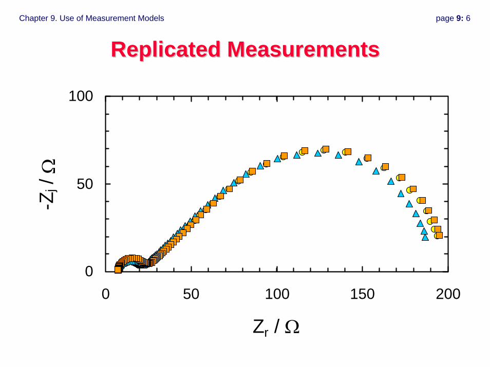
Chapter 9. Use of Measurement Models page 9: 6
Replicated MeasurementsReplicated Measurements
0
50
100
0 50 100 150 200
Zr / Ω
-Zj /
Ω
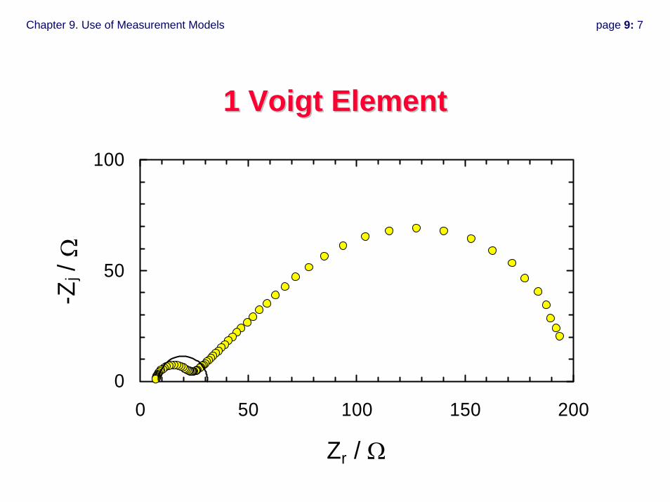
Chapter 9. Use of Measurement Models page 9: 7
1 Voigt Element1 Voigt Element
0
50
100
0 50 100 150 200
Zr / Ω
-Zj /
Ω
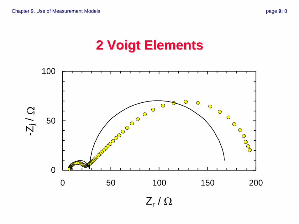
Chapter 9. Use of Measurement Models page 9: 8
2 Voigt Elements2 Voigt Elements
0
50
100
0 50 100 150 200
Zr / Ω
-Zj /
Ω
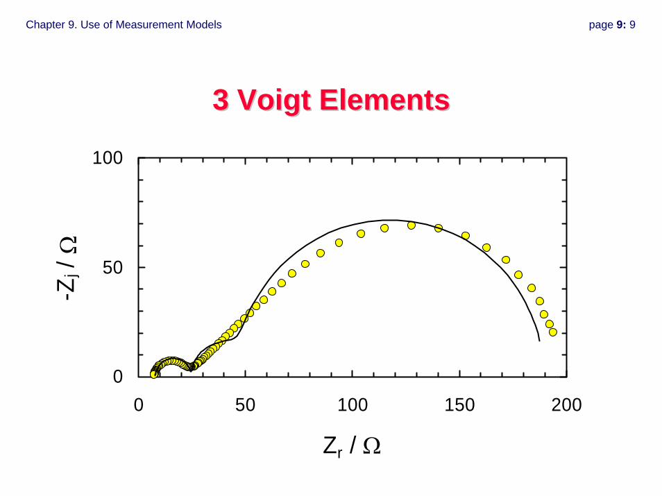
Chapter 9. Use of Measurement Models page 9: 9
3 Voigt Elements3 Voigt Elements
0
50
100
0 50 100 150 200
Zr / Ω
-Zj /
Ω
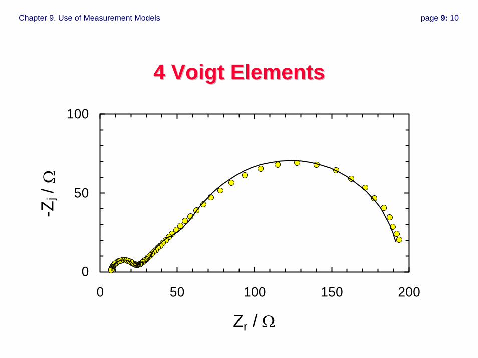
Chapter 9. Use of Measurement Models page 9: 10
4 Voigt Elements4 Voigt Elements
0
50
100
0 50 100 150 200
Zr / Ω
-Zj /
Ω
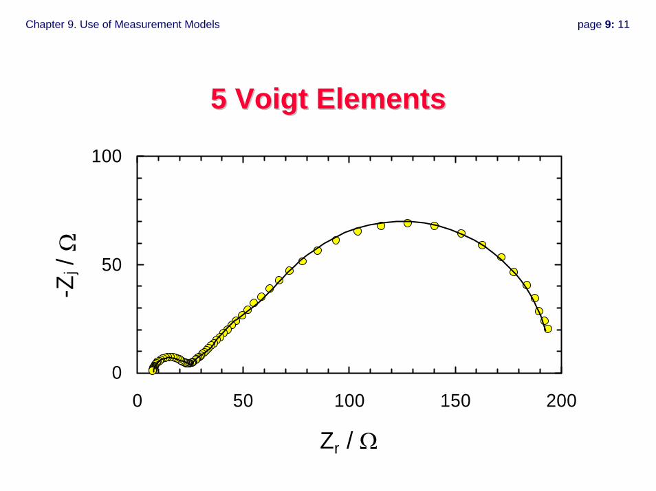
Chapter 9. Use of Measurement Models page 9: 11
5 Voigt Elements5 Voigt Elements
0
50
100
0 50 100 150 200
Zr / Ω
-Zj /
Ω
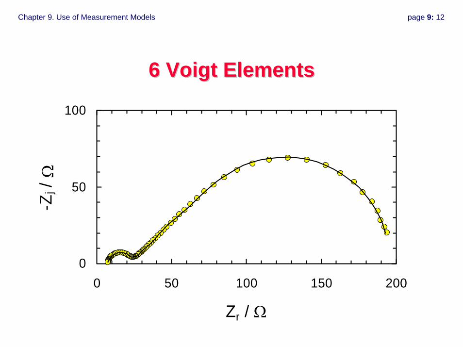
Chapter 9. Use of Measurement Models page 9: 12
6 Voigt Elements6 Voigt Elements
0
50
100
0 50 100 150 200
Zr / Ω
-Zj /
Ω
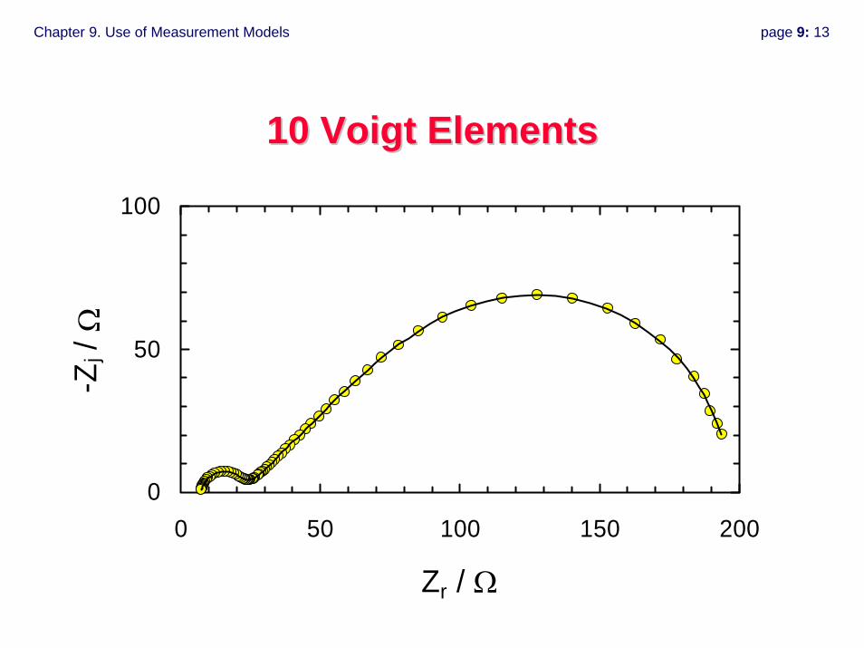
Chapter 9. Use of Measurement Models page 9: 13
10 Voigt Elements10 Voigt Elements
0
50
100
0 50 100 150 200
Zr / Ω
-Zj /
Ω
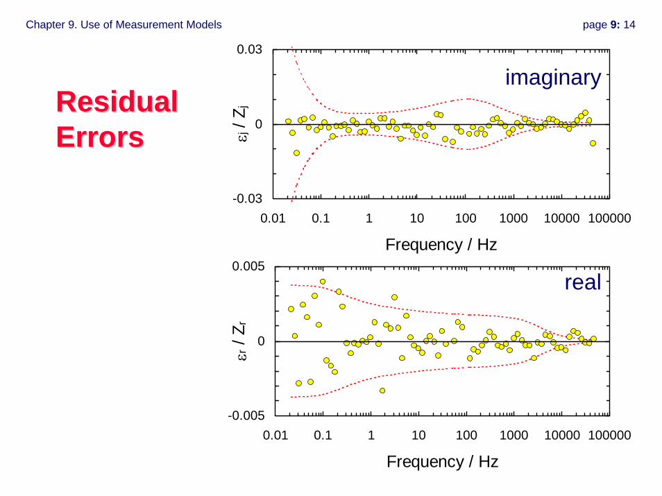
Chapter 9. Use of Measurement Models page 9: 14
Residual Residual ErrorsErrors
-0.005
0
0.005
0.01 0.1 1 10 100 1000 10000 100000
Frequency / Hz
εr /
Z r
-0.03
0
0.03
0.01 0.1 1 10 100 1000 10000 100000
Frequency / Hzεj
/ Zj
imaginary
real
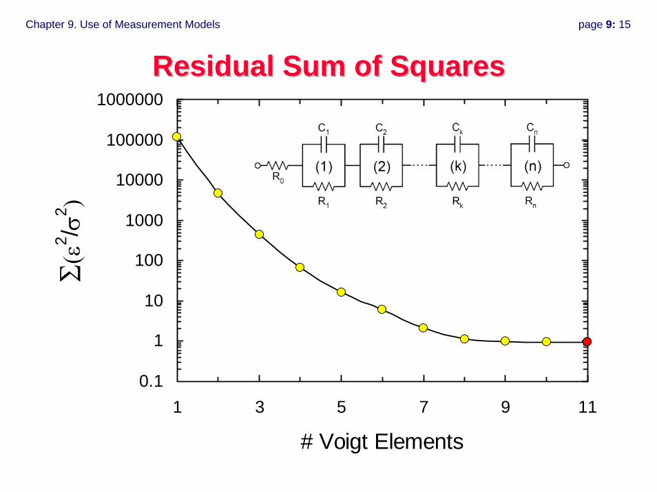
Chapter 9. Use of Measurement Models page 9: 15
Residual Sum of SquaresResidual Sum of Squares
0.1
1
10
100
1000
10000
100000
1000000
1 3 5 7 9 11
# Voigt Elements
Σ(ε2 / σ
2 )
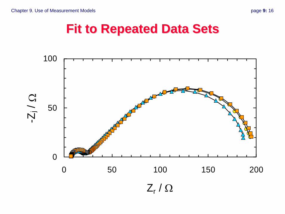
Chapter 9. Use of Measurement Models page 9: 16
Fit to Repeated Data SetsFit to Repeated Data Sets
0
50
100
0 50 100 150 200
Zr / Ω
-Zj /
Ω
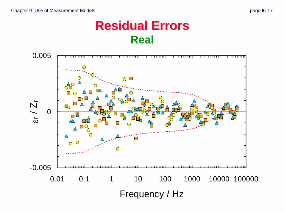
Chapter 9. Use of Measurement Models page 9: 17
Residual ErrorsResidual ErrorsReal
-0.005
0
0.005
0.01 0.1 1 10 100 1000 10000 100000
Frequency / Hz
εr /
Z r
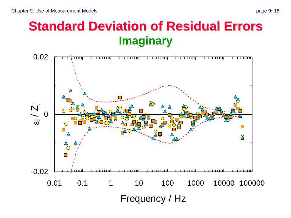
Chapter 9. Use of Measurement Models page 9: 18
Standard Deviation of Residual ErrorsStandard Deviation of Residual ErrorsImaginary
-0.02
0
0.02
0.01 0.1 1 10 100 1000 10000 100000
Frequency / Hz
εj / Z
j
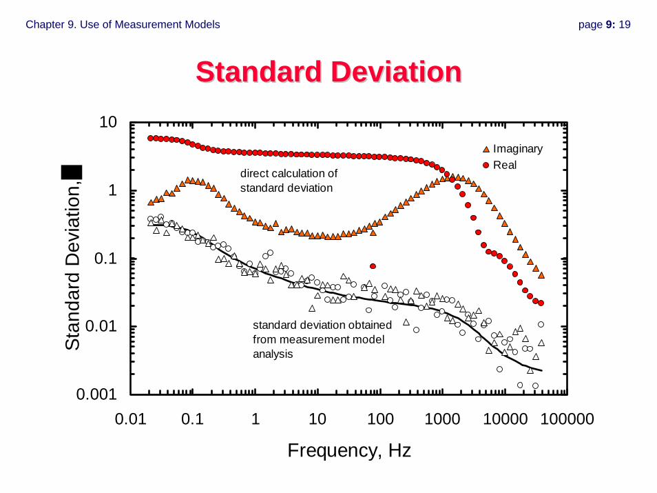
Chapter 9. Use of Measurement Models page 9: 19
Standard DeviationStandard Deviation
0.001
0.01
0.1
1
10
0.01 0.1 1 10 100 1000 10000 100000
Frequency, Hz
Stan
dard
Dev
iatio
n,
ImaginaryReal
direct calculation of standard deviation
standard deviation obtained from measurement model analysis
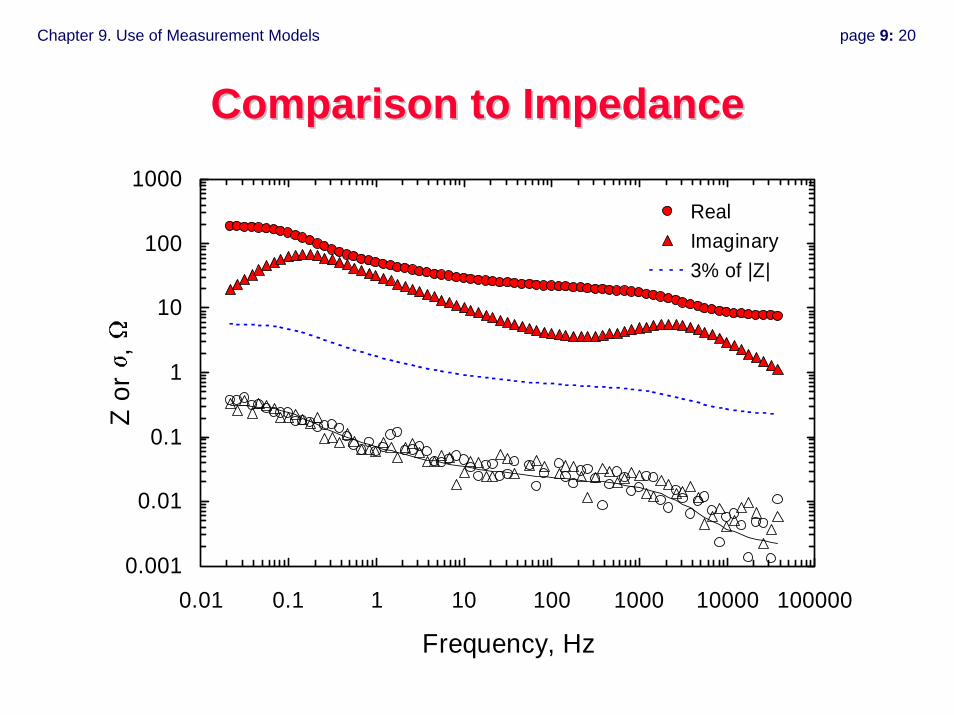
Chapter 9. Use of Measurement Models page 9: 20
Comparison to ImpedanceComparison to Impedance
0.001
0.01
0.1
1
10
100
1000
0.01 0.1 1 10 100 1000 10000 100000
Frequency, Hz
Z or
,
RealImaginary3% of |Z|
Chapter 9. Use of Measurement Models page 9: 21
Identification of Bias Component of Error Structure
How?• Fit measurement model to real
component:– predict imaginary component.– Use Monte Carlo calculations to
estimate confidence interval.• Fit measurement model to
imaginary component:– predict real component.– Use Monte Carlo calculations to
estimate confidence interval.
Why?• Identify suitable
frequency range for regression.
• Improve experimental design.
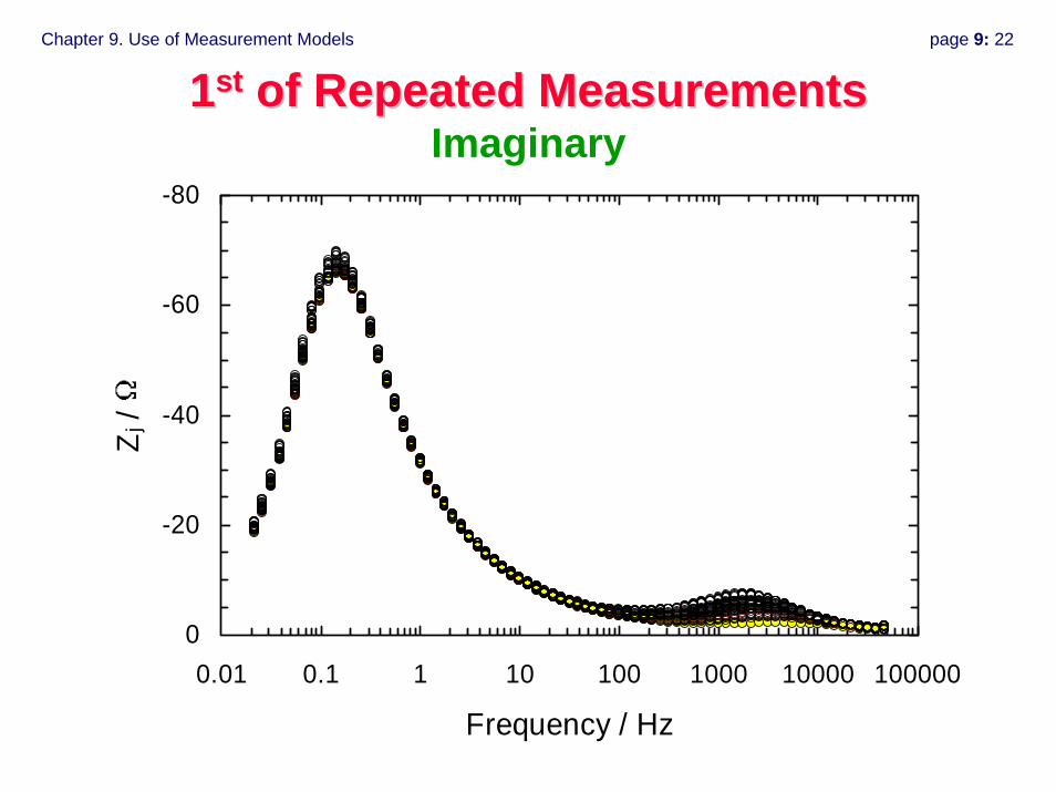
Chapter 9. Use of Measurement Models page 9: 22
11stst of Repeated Measurementsof Repeated MeasurementsImaginary
-80
-60
-40
-20
00.01 0.1 1 10 100 1000 10000 100000
Frequency / Hz
Z j /
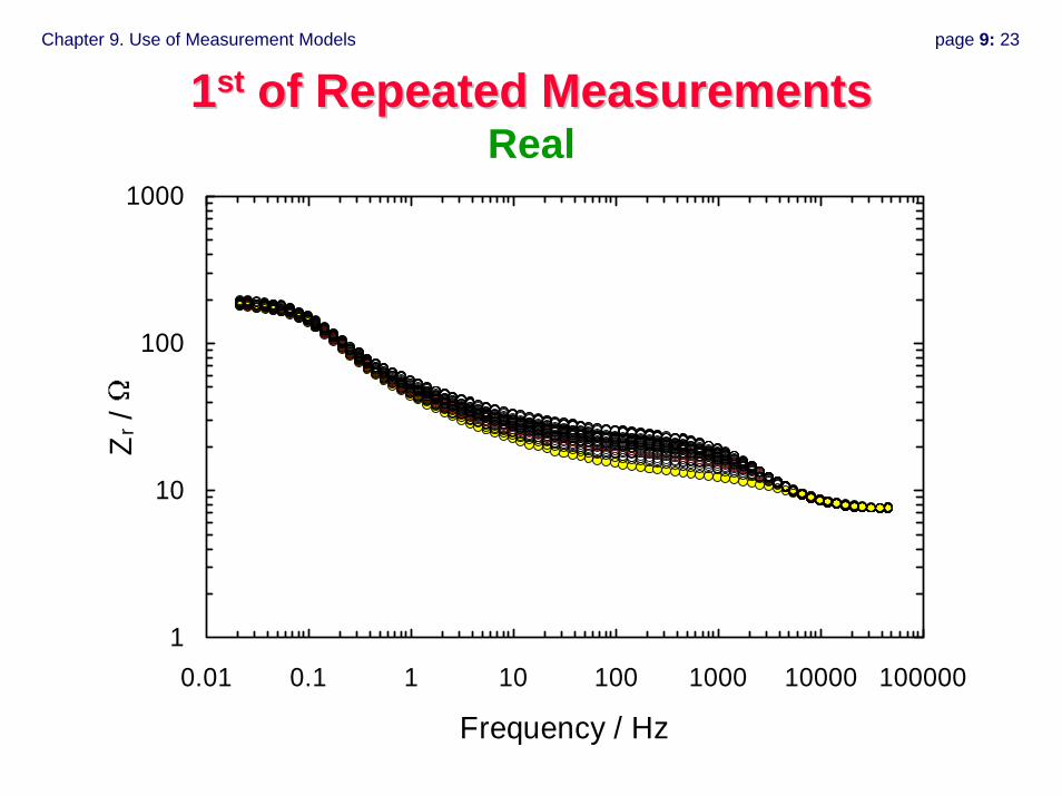
Chapter 9. Use of Measurement Models page 9: 23
11stst of Repeated Measurementsof Repeated MeasurementsReal
1
10
100
1000
0.01 0.1 1 10 100 1000 10000 100000
Frequency / Hz
Z r /
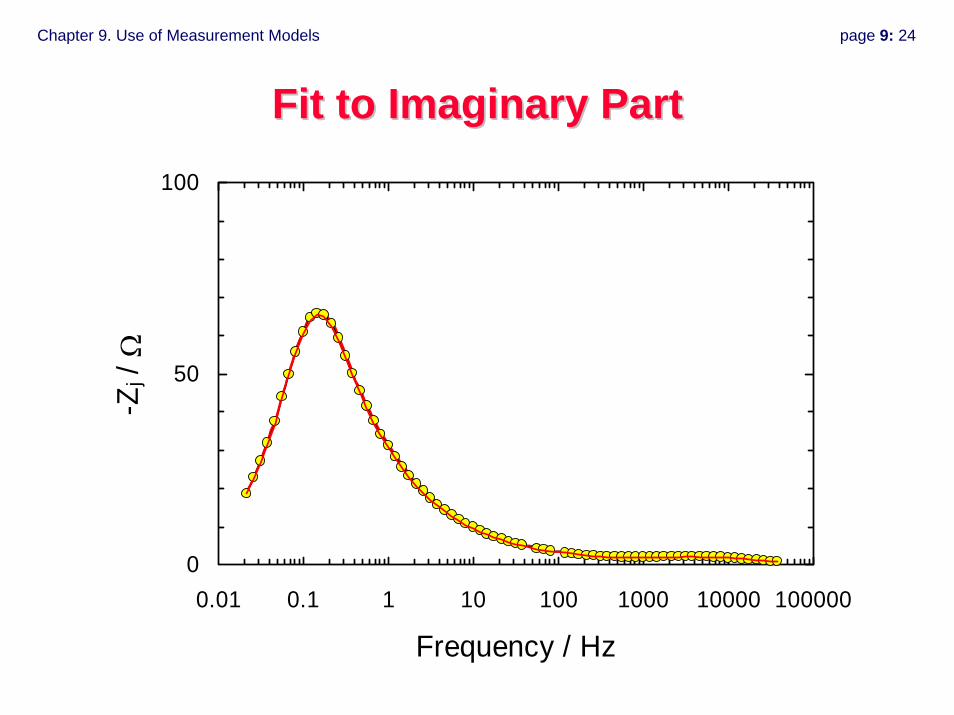
Chapter 9. Use of Measurement Models page 9: 24
Fit to Imaginary PartFit to Imaginary Part
0
50
100
0.01 0.1 1 10 100 1000 10000 100000
Frequency / Hz
-Zj /
Ω
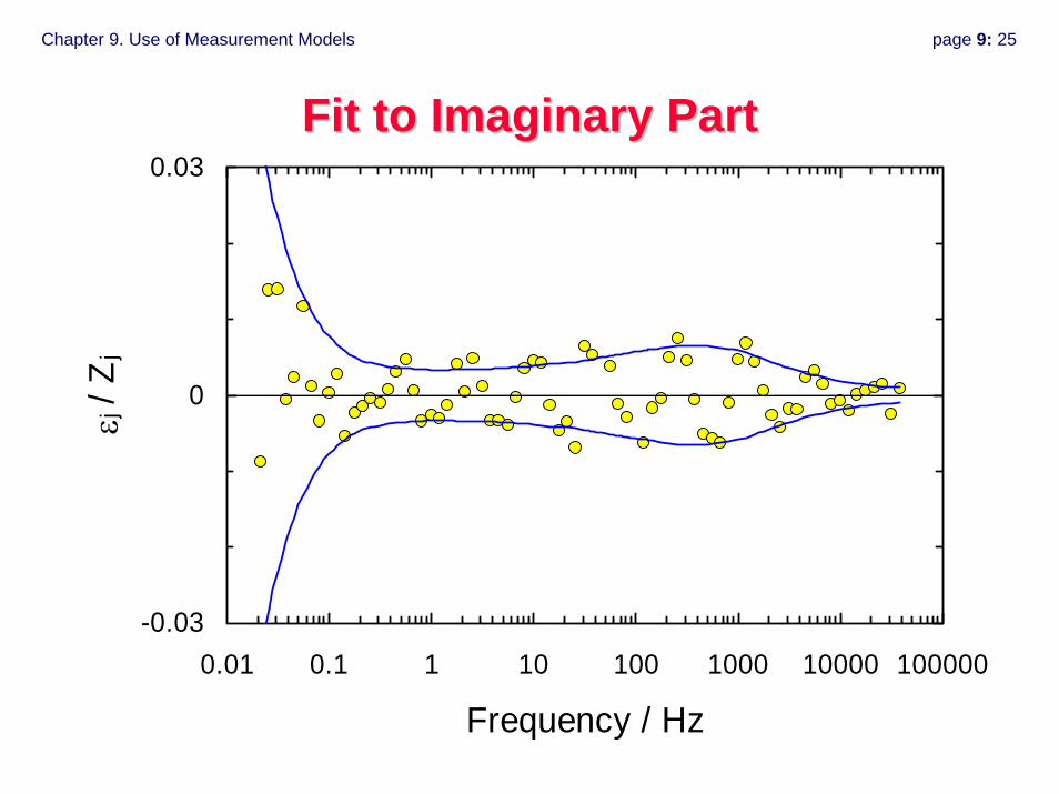
Chapter 9. Use of Measurement Models page 9: 25
Fit to Imaginary PartFit to Imaginary Part
-0.03
0
0.03
0.01 0.1 1 10 100 1000 10000 100000
Frequency / Hz
εj / Z
j
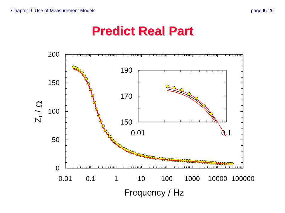
Chapter 9. Use of Measurement Models page 9: 26
Predict Real PartPredict Real Part
0
50
100
150
200
0.01 0.1 1 10 100 1000 10000 100000
Frequency / Hz
Z r / Ω
150
170
190
0.01 0.1
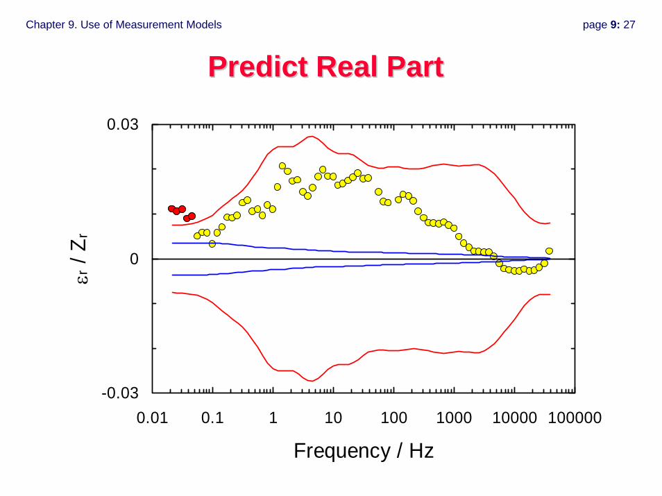
Chapter 9. Use of Measurement Models page 9: 27
Predict Real PartPredict Real Part
-0.03
0
0.03
0.01 0.1 1 10 100 1000 10000 100000
Frequency / Hz
εr /
Z r
Chapter 9. Use of Measurement Models page 9: 28
Validation of Measurement Model Validation of Measurement Model ApproachApproach
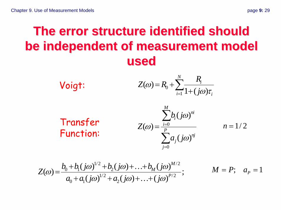
Chapter 9. Use of Measurement Models page 9: 29
The error structure identified should The error structure identified should be independent of measurement model be independent of measurement model
usedused
01
( )1 ( )
Ni
i i
RZ Rj
ωω τ=
= ++∑Voigt:
0
0
( )( )
( )
Mni
iiP
njj
j
b jZ
a j
ωω
ω
=
=
=∑
∑Transfer Function:
1/ 2n =
1/2 /20 1 2
1/2 /20 1 2
( ) ( ) ( )( ) ;( ) ( ) ( )
MM
P
b b j b j b jZa a j a j j
ω ω ωωω ω ω
+ + + +=
+ + + +……
; 1PM P a= =
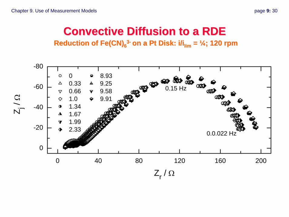
Chapter 9. Use of Measurement Models page 9: 30
Convective Diffusion to a RDEConvective Diffusion to a RDEReduction of Fe(CN)Reduction of Fe(CN)66
33-- on a Pt Disk: on a Pt Disk: i/ii/ilimlim = = ¼¼; 120 rpm; 120 rpm
0 40 80 120 160 200
0
-20
-40
-60
-80 0 8.93 0.33 9.25 0.66 9.58 1.0 9.91 1.34 1.67 1.99 2.33 0.0.022 Hz
Z j / Ω
Zr / Ω
0.15 Hz
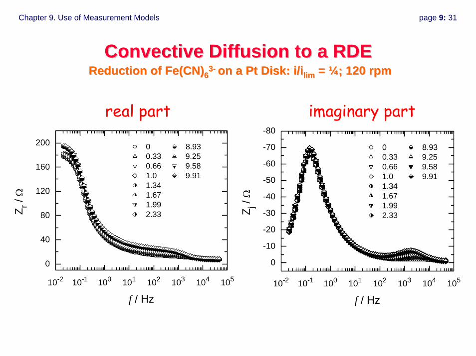
Chapter 9. Use of Measurement Models page 9: 31
10-2 10-1 100 101 102 103 104 105
0
40
80
120
160
200 0 8.93 0.33 9.25 0.66 9.58 1.0 9.91 1.34 1.67 1.99 2.33
Z r / Ω
f / Hz10-2 10-1 100 101 102 103 104 105
0
-10
-20
-30
-40
-50
-60
-70
-80
0 8.93 0.33 9.25 0.66 9.58 1.0 9.91 1.34 1.67 1.99 2.33
Z j / Ω
f / Hz
Convective Diffusion to a RDEConvective Diffusion to a RDEReduction of Fe(CN)Reduction of Fe(CN)66
33-- on a Pt Disk: on a Pt Disk: i/ii/ilimlim = = ¼¼; 120 rpm; 120 rpm
real part imaginary part
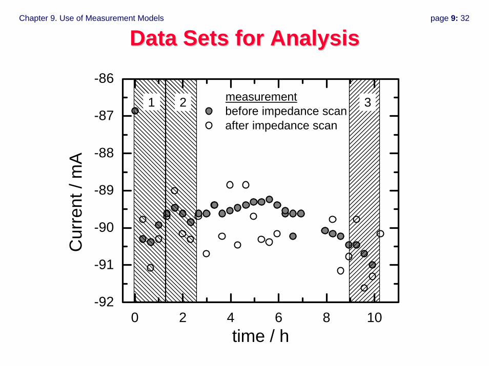
Chapter 9. Use of Measurement Models page 9: 32
Data Sets for AnalysisData Sets for Analysis
0 2 4 6 8 10-92
-91
-90
-89
-88
-87
-86 measurement
before impedance scan after impedance scan
3 2
Cur
rent
/ m
A
time / h
1
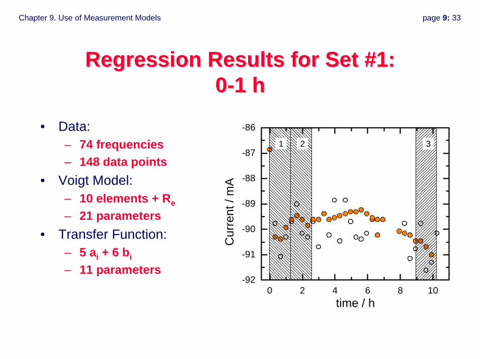
Chapter 9. Use of Measurement Models page 9: 33
Regression Results for Set #1: Regression Results for Set #1: 00--1 h1 h
• Data: – 74 frequencies – 148 data points
• Voigt Model: – 10 elements + Re
– 21 parameters• Transfer Function:
– 5 ai + 6 bi
– 11 parameters0 2 4 6 8 10
-92
-91
-90
-89
-88
-87
-86
3 2
Cur
rent
/ m
A
time / h
1
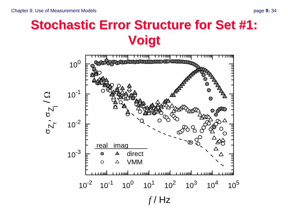
Chapter 9. Use of Measurement Models page 9: 34
Stochastic Error Structure for Set #1: Stochastic Error Structure for Set #1: VoigtVoigt
10-2 10-1 100 101 102 103 104 105
10-3
10-2
10-1
100
real imag direct VMM
σ Z
r, σZ j /
Ω
f / Hz
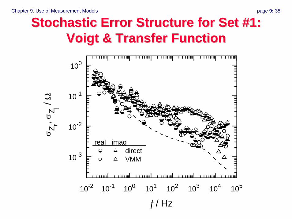
Chapter 9. Use of Measurement Models page 9: 35
Stochastic Error Structure for Set #1: Stochastic Error Structure for Set #1: Voigt & Transfer FunctionVoigt & Transfer Function
10-2 10-1 100 101 102 103 104 105
10-3
10-2
10-1
100
real imag direct VMM
σ Z
r, σZ j /
Ω
f / Hz
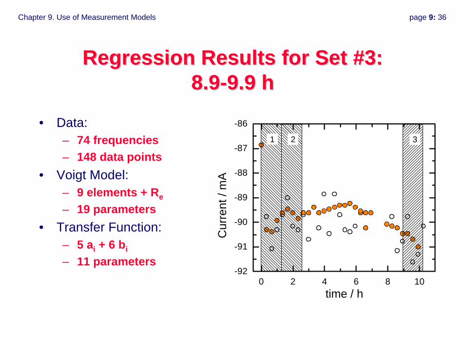
Chapter 9. Use of Measurement Models page 9: 36
Regression Results for Set #3: Regression Results for Set #3: 8.98.9--9.9 h9.9 h
• Data: – 74 frequencies – 148 data points
• Voigt Model: – 9 elements + Re
– 19 parameters• Transfer Function:
– 5 ai + 6 bi
– 11 parameters0 2 4 6 8 10
-92
-91
-90
-89
-88
-87
-86
3 2
Cur
rent
/ m
A
time / h
1
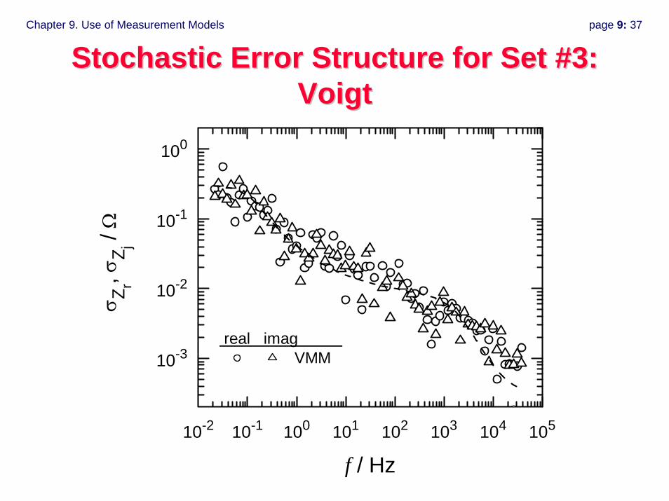
Chapter 9. Use of Measurement Models page 9: 37
Stochastic Error Structure for Set #3: Stochastic Error Structure for Set #3: VoigtVoigt
10-2 10-1 100 101 102 103 104 105
10-3
10-2
10-1
100
real imag VMM
σ Z
r, σZ j /
Ω
f / Hz
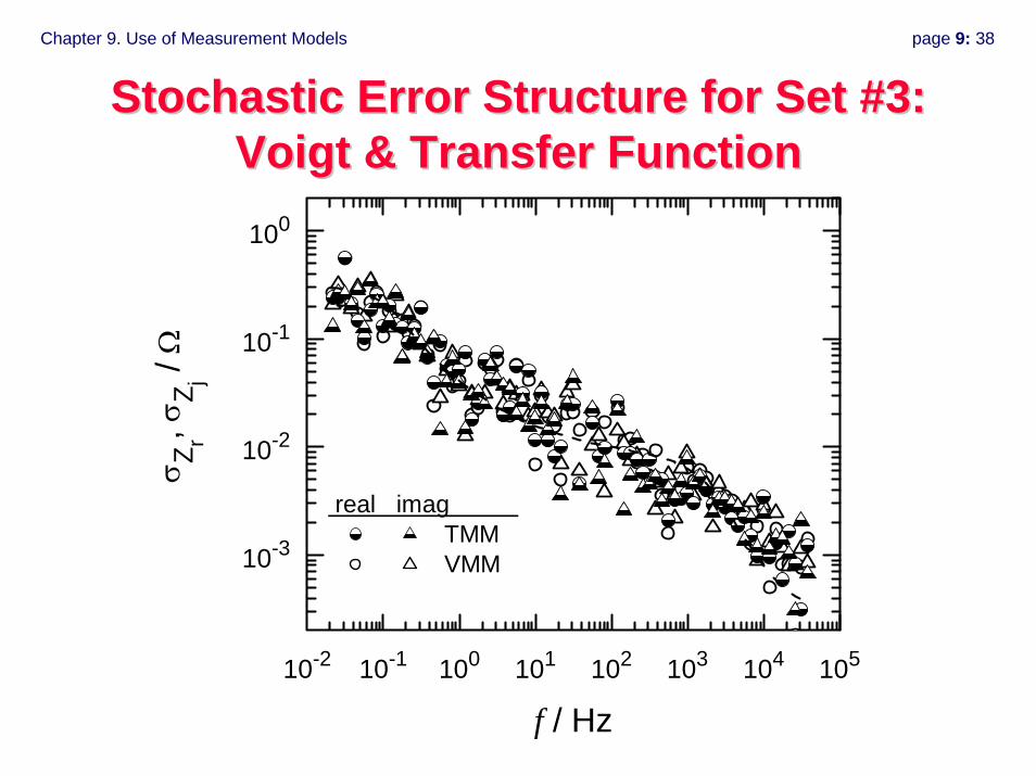
Chapter 9. Use of Measurement Models page 9: 38
Stochastic Error Structure for Set #3: Stochastic Error Structure for Set #3: Voigt & Transfer FunctionVoigt & Transfer Function
10-2 10-1 100 101 102 103 104 105
10-3
10-2
10-1
100
real imag TMM VMM
σ Z
r, σZ j /
Ω
f / Hz
Chapter 9. Use of Measurement Models page 9: 39
Identification of Stochastic Component Identification of Stochastic Component of Error Structureof Error Structure
• Direct evaluation of standard deviation includes significant contributions from changes in system behavior
• The error structure identified was independent of measurement model used
• Selection of measurement model– Ease of identification of initial parameters → Voigt– Number of parameters → Transfer Function
Chapter 9. Use of Measurement Models page 9: 40
Evaluation of Consistency with the Evaluation of Consistency with the KramersKramers--Kronig relationsKronig relations
• Approach– Fit measurement model to imaginary component– Use experimental variance to weight regression– Predict real component– Compare prediction to measured data– Use Monte Carlo calculations to estimate confidence interval
• Assumption– Measurement model satisfies the Kramers-Kronig relations
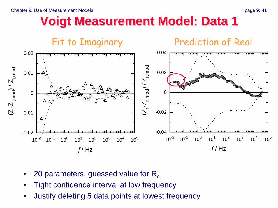
Chapter 9. Use of Measurement Models page 9: 41
Voigt Measurement Model: Data 1Voigt Measurement Model: Data 1
10-2 10-1 100 101 102 103 104 105-0.02
-0.01
0
0.01
0.02
(Zj-Z
j,mod
) / Z
j,mod
f / Hz
Fit to Imaginary
10-2 10-1 100 101 102 103 104 105-0.04
-0.02
0
0.02
0.04
• 20 parameters, guessed value for Re
• Tight confidence interval at low frequency• Justify deleting 5 data points at lowest frequency
(Zr-Z
r,mod
) / Z
r,mod
f / Hz
Prediction of Real
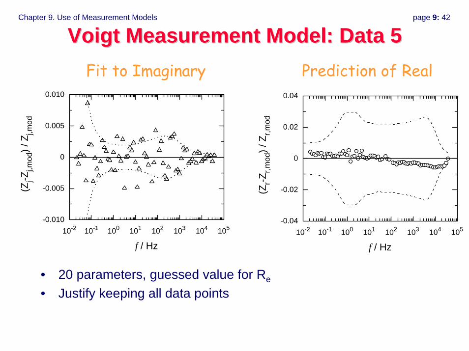
Chapter 9. Use of Measurement Models page 9: 42
Voigt Measurement Model: Data 5Voigt Measurement Model: Data 5
• 20 parameters, guessed value for Re
• Justify keeping all data points
10-2 10-1 100 101 102 103 104 105-0.010
-0.005
0
0.005
0.010
(Zj-Z
j,mod
) / Z
j,mod
f / Hz
Fit to Imaginary
10-2 10-1 100 101 102 103 104 105-0.04
-0.02
0
0.02
0.04
(Zr-Z
r,mod
) / Z
r,mod
f / Hz
Prediction of Real
Chapter 9. Use of Measurement Models page 9: 43
Interpretation of Impedance SpectraInterpretation of Impedance Spectra
• Physical insight and knowledge of error structure– stochastic component
• weighting• determination of model adequacy• experimental design
– bias component• suitable frequency range• experimental design
• Measurement model approach is general– electrochemical impedance spectroscopies– optical spectroscopies– mechanical spectroscopies

Chapter 9. Use of Measurement Models page 9: 44
Chapter 10. Conclusions page 10: 1
Electrochemical Impedance Electrochemical Impedance SpectroscopySpectroscopy
Chapter 10. ConclusionsChapter 10. Conclusions
• Overview of Course• Credits
© Mark E. Orazem, 2000-2008. All rights reserved.
Chapter 10. Conclusions page 10: 2
Overview of CourseOverview of Course
• Chapter 1. Introduction • Chapter 2. Motivation • Chapter 3. Impedance Measurement • Chapter 4. Representations of Impedance Data• Chapter 5. Development of Process Models• Chapter 6. Regression Analysis• Chapter 7. Error Structure• Chapter 8. Kramers-Kronig Relations• Chapter 9. Use of Measurement Models• Chapter 10. Conclusions• Chapter 11. Suggested Reading• Chapter 12. Notation
Chapter 10. Conclusions page 10: 3
Impedance SpectroscopyImpedance Spectroscopy• Electrochemical measurement of macroscopic properties• Example of a generalized transfer-function measurement• Can be used to extract contributions of
– electrode reactions– mass transfer– surface layers
• Can be used to estimate – reaction rates– transport properties
• Interpretation of data– graphical representations– regression– process models – error analysis

Chapter 10. Conclusions page 10: 4Integrated ApproachIntegrated Approach
Chapter 10. Conclusions page 10: 5
AcknowledgementsAcknowledgements• Students
– University of Florida• P. Agarwal, M. Durbha, S. Carson, M. Membrino, P. Shukla, V. Huang, S. Roy, B. Hirschorn,
S-L Wu– CNRS
• T. El Moustafid, I. Frateur, H. G. de Melo– CIRIMAT
• J-B Jorcin • Collaborators
– University of South Florida• L. García-Rubio
– University of Florida • O. Crisalle
– CNRS, Paris• B. Tribollet, C. Deslouis, H. Takenouti, V. Vivier
– CIRIMAT, Toulouse• N. Pébère
– CNR, Italy• M. Musiani
• Funding– NSF, ONR, SC Johnson, CNRS, NASA
• Other– The Electrochemical Society– The Fuel Cell Seminar

Chapter 10. Conclusions page 10: 6
Chapter 11. Suggested Reading page 11: 1
Electrochemical Impedance Electrochemical Impedance SpectroscopySpectroscopy
Chapter 11. Suggested Reading Chapter 11. Suggested Reading
• General• Process Models• Orazem group work on Fuel Cells• Measurement Models• CPE• Plotting
© Mark E. Orazem, 2000-2008. All rights reserved.
Chapter 11. Suggested Reading page 11: 2
Suggested ReadingSuggested ReadingGeneralGeneral
• J. R. Macdonald, editor, Impedance Spectroscopy Emphasizing Solid Materials and Analysis, John Wiley and Sons, New York, 1987.
• E. Barsoukov and J. R. Macdonald, editors, Impedance Spectroscopy: Theory, Experiment, and Applications, 2nd Edition, John Wiley and Sons, New York, 2005.
• C. Gabrielli, Use and Applications of Electrochemical Impedance Techniques, Technical Report, Schlumberger, Farnborough, England, 1990.
• D. Macdonald, Transient Techniques in Electrochemistry, Plenum Press, NY, 1977.
• M. E. Orazem and B. Tribollet, Electrochemical Impedance Spectroscopy, John Wiley and Sons, New York, 2008.
• Other Sources– See instrument vendor websites for for application notes.
Chapter 11. Suggested Reading page 11: 3
Suggested ReadingSuggested ReadingProcess ModelsProcess Models
• A. Lasia, “Electrochemical Impedance Spectroscopy and Its Applications,” Modern Aspects of Electrochemistry, 32, R. E. White, J. O'M. Bockris and B. E. Conway, editors, Plenum Press, New York, 1999, 143-248.
• C. Deslouis and B. Tribollet, Flow Modulation Techniques in Electrochemistry, Advances in Electrochemical Science and Engineering, 2, H. Gerischer and C. W. Tobias, editors, VCH, Weinheim, 1992, 205-264.
• M. E. Orazem, “Tutorial: Application of Mathematical Models for Interpretation of Impedance Spectra,” Tutorials in Electrochemical Engineering - Mathematical Modeling, PV 99-14, R.F. Savinell, A.C. West, J.M. Fenton and J. Weidner, editors, Electrochemical Society, Inc., Pennington, N.J., 68-99, 1999.
• B. Tribollet, Look-up Tables for Rotating Disk Electrode, April 28, 2000, http://www.ccr.jussieu.fr/lple/EnglishVersion.html

Chapter 11. Suggested Reading page 11: 4
• S. K. Roy and M. E. Orazem, “Error Analysis of the Impedance Response of PEM Fuel Cells,” Journal of the Electrochemical Society,154 (2007), B883-B891
• S. K. Roy and M. E. Orazem, “Deterministic Impedance Models for Interpretation of Low-Frequency Inductive Loops in PEM Fuel Cells,” in Proton Exchange Membrane Fuel Cells 6, T. Fuller, C. Bock, S. Cleghorn, H. Gasteiger, T. Jarvi, M. Mathias, M. Murthy, T. Nguyen, V. Ramani, E. Stuve, T. Zawodzinski, editors, ECS Transactions, 3:1(2006), 1031-1040.
• S. K. Roy and M. E. Orazem, “Stochastic Analysis of Flooding in PEM Fuel Cells by Electrochemical Impedance Spectroscopy,” in Proton Exchange Membrane Fuel Cells 7, T. Fuller, H. Gasteiger, S. Cleghorn, V. Ramani, T. Zhao, T. Nguyen, A. Haug, C. Bock, C. Lamy, and K. Ota, editors, Electrochemical Society Transactions, 11:1 (2007), 485-495.
• S. K. Roy, M. E. Orazem, and B. Tribollet “Interpretation of Low-Frequency Inductive Loops in PEM Fuel Cells,” Journal of the Electrochemical Society, 154 (2007), B1378-B1388.
Suggested ReadingSuggested ReadingOrazem group work on Fuel CellsOrazem group work on Fuel Cells
Chapter 11. Suggested Reading page 11: 5
Suggested ReadingSuggested ReadingCPECPE
• G. J. Brug, A. L. G. van den Eeden, M. Sluyters-Rehbach, and J. H. Sluyters, “The Analysis of Electrode Impedances Complicated by the Presence of a Constant Phase Element,” Journal of ElectroanalyticChemistry, 176 (1984), 275-295.
• V. Huang, V. Vivier, M. Orazem, N. Pébère, and B. Tribollet, “The Apparent CPE Behavior of an Ideally Polarized Blocking Electrode: A Global and Local Impedance Analysis,” Journal of the Electrochemical Society, 154 (2007), C81-C88.
• V. Huang, V. Vivier, M. Orazem, I. Frateur, and B. Tribollet, “The Global and Local Impedance Response of a Blocking Disk Electrode with Local CPE Behavior,” Journal of the Electrochemical Society, 154(2007), C89-C98.
• V. Huang, V. Vivier, M. Orazem, N. Pébère, and B. Tribollet, “The Apparent CPE Behavior of a Disk Electrode with Faradaic Reactions: A Global and Local Impedance Analysis,” Journal of the Electrochemical Society, 154 (2007), C99-C107.
Chapter 11. Suggested Reading page 11: 6
Suggested ReadingSuggested ReadingMeasurement ModelsMeasurement Models
• P. Agarwal, M. E. Orazem, and L. H. García-Rubio, "Measurement Models for Electrochemical Impedance Spectroscopy: 1. Demonstration of Applicability," Journal of the Electrochemical Society, 139 (1992), 1917-1927.
• P. Agarwal, Oscar D. Crisalle, M. E. Orazem, and L. H. García-Rubio, "Measurement Models for Electrochemical Impedance Spectroscopy: 2. Determination of the Stochastic Contribution to the Error Structure," Journal of the Electrochemical Society, 142 (1995), 4149-4158.
• P. Agarwal, M. E. Orazem, and L. H. García-Rubio, "Measurement Models for Electrochemical Impedance Spectroscopy: 3. Evaluation of Consistency with the Kramers-Kronig Relations,” Journal of the Electrochemical Society, 142 (1995), 4159-4168.
• M. E. Orazem “A Systematic Approach toward Error Structure Identification for Impedance Spectroscopy,” Journal of Electroanalytical Chemistry, 572 (2004), 317-327.
Chapter 11. Suggested Reading page 11: 7
Suggested ReadingSuggested ReadingPlottingPlotting
• M. Orazem, B. Tribollet, and N. Pébère, “Enhanced Graphical Representation of Electrochemical Impedance Data,” Journal of the Electrochemical Society, 153 (2006), B129-B136.
EElleeccttrroocchheemmiiccaall IImmppeeddaannccee
SSppeeccttrroossccooppyy
CChhaapptteerr 1122.. NNoottaattiioonn
• Roman • Greek

Chapter 12. Notation page 12: 2
Roman a coefficient in the Cochran expansion for velocity, 0.51023 a =
b coefficient in the Cochran expansion for velocity, -0.61592 b =
ic concentration of reacting species , mol/cm3 i
ic steady-state value of the concentration of reacting species , mol/cm3 i
ic Oscillating component of the concentration of reacting species , mol/cm3 i
,oic concentration of species on the electrode surface, mol/cm3 i
,oic steady-state value of the concentration of species on the electrode surface, mol/cm3 i
,oic Oscillating component of the concentration of species on the electrode surface, mol/cm3 i
∞c bulk concentration of the reacting species, mol/cm3
dC double layer capacitance, F/cm2
dlC double layer capacitance, F/cm2
iD diffusion coefficient of species , cm2/s i
f arbitrary function, e.g., ( ),f ii f V c=
F Faraday’s constant, C/equiv
i Total current density, A/cm2
i Steady-state total current density, A/cm2

Chapter 12. Notation page 12: 3
i Oscillating component of total current density, A/cm2
fi Faradic current density, A/cm2
fi Steady-state Faradic current density, A/cm2
fi Oscillating component of Faradic current density, A/cm2
0i Exchange current density, A/cm2
j imaginary number, 1−
Ak rate constant for reaction identified by index A (units depend on reaction stoichiometry)
dimensionless frequency,
1 13 31/3
2 2
9 9 Sci ii
Ka D a
ω ν ω⎛ ⎞ ⎛ ⎞= =⎜ ⎟ ⎜ ⎟Ω Ω ⎝ ⎠⎝ ⎠ K
iM notation for species i
n number of electrons produced when one reactant ion or molecule reacts
R universal gas constant, J/mol/K
eR Ohmic resistance, Ω cm2
,t AR Charge-transfer resistance associated with reaction A, Ω cm2
r radial coordinate, cm
0r radius of disk, cm
is stoichiometric coefficient for species , ( for a reactant and i 0is > 0is < for a product)
Chapter 12. Notation page 12: 4
Sci Schmidt number, Sc /i iDν=
T electrolyte temperature, K
t time, s
zr vv , radial and axial velocity components, respectively, cm/s
V potential, V
V steady-state potential, V
V oscillating contribution to potential, V
Z impedance, Ω cm2
z axial position, cm
dz diffusion impedance, Ω cm2
iz charge for species i
Greek α coefficient used in the exponent for a constant-phase element. When 0α = , the element behaves as an ideal capacitor in
parallel with a resistor.
Aα apparent transfer coefficient for reaction A
Aβ Tafel slope for reaction A, V
iγ Fractional surface coverage by species i
Chapter 12. Notation page 12: 5
Γ Maximum surface coverage
iδ characteristic diffusion length for species i
θ homogeneous solution to the oscillating dimensionless convective diffusion equation
(0)θ ′ derivative of the solution to the oscillating dimensionless convective diffusion equation evaluated at the electrode surface
η surface overpotential, V
∞κ solution conductivity, (Ω cm)-1
characteristic length for a finite-length diffusion layer, 1/ 3 2 / 32.598 /iDν= Ω
μ viscosity, g/cm s
ν kinematic viscosity, /ν μ ρ= , cm2/s
ρ density, g/cm3
τ finite-length diffusion time constant, 2 / iDτ =
ξ normalized axial position, / izξ δ=
Φ ohmic potential, V
ω frequency of perturbation, rad/s
Ω rotation speed, rad/sec