Lenient Multi-Agent Deep Reinforcement LearningGregory Palmer

University of LiverpoolUnited Kingdom

G.J.Palmer@liverpool.ac.uk

Karl TuylsDeepMind and University of Liverpool

United Kingdomkarltuyls@google.com

Daan BloembergenCentrum Wiskunde & Informatica

The Netherlandsd.bloembergen@cwi.nl

Rahul SavaniUniversity of Liverpool

United KingdomRahul.Savani@liverpool.ac.uk

ABSTRACTMuch of the success of single agent deep reinforcement learning(DRL) in recent years can be attributed to the use of experiencereplay memories (ERM), which allow Deep Q-Networks (DQNs)to be trained efficiently through sampling stored state transitions.However, care is required when using ERMs for multi-agent deepreinforcement learning (MA-DRL), as stored transitions can becomeoutdated because agents update their policies in parallel [11]. Inthis work we apply leniency [23] to MA-DRL. Lenient agents mapstate-action pairs to decaying temperature values that control theamount of leniency applied towards negative policy updates thatare sampled from the ERM. This introduces optimism in the value-function update, and has been shown to facilitate cooperation intabular fully-cooperative multi-agent reinforcement learning prob-lems.We evaluate our Lenient-DQN (LDQN) empirically against therelated Hysteretic-DQN (HDQN) algorithm [22] as well as a mod-ified version we call scheduled-HDQN, that uses average rewardlearning near terminal states. Evaluations take place in extendedvariations of the Coordinated Multi-Agent Object TransportationProblem (CMOTP) [8] which include fully-cooperative sub-tasksand stochastic rewards. We find that LDQN agents are more likelyto converge to the optimal policy in a stochastic reward CMOTPcompared to standard and scheduled-HDQN agents.

KEYWORDSDistributed problem solving; Multiagent learning; Deep learning

1 INTRODUCTIONThe field of deep reinforcement learning has seen a great numberof successes in recent years. Deep reinforcement learning agentshave been shown to master numerous complex problem domains,ranging from computer games [17, 21, 26, 33] to robotics tasks [10,12]. Much of this success can be attributed to using convolutionalneural network (ConvNet) architectures as function approximators,allowing reinforcement learning agents to be applied to domainswith large or continuous state and action spaces. ConvNets are oftentrained to approximate policy and value functions through sampling

Proc. of the 17th International Conference on Autonomous Agents and Multiagent Systems(AAMAS 2018), M. Dastani, G. Sukthankar, E. Andre, S. Koenig (eds.), July 2018, Stockholm,Sweden© 2018 International Foundation for Autonomous Agents and Multiagent Systems(www.ifaamas.org). All rights reserved.https://doi.org/doi

past state transitions stored by the agent inside an experience replaymemory (ERM).

Recently the sub-field of multi-agent deep reinforcement learn-ing (MA-DRL) has received an increased amount of attention. Multi-agent reinforcement learning is known for being challenging evenin environments with only two implicit learning agents, lackingthe convergence guarantees present in most single-agent learningalgorithms [5, 20]. One of the key challenges faced within multi-agent reinforcement learning is the moving target problem: Givenan environment with multiple agents whose rewards depend oneach others’ actions, the difficulty of finding optimal policies foreach agent is increased due to the policies of the agents being nonstationary [7, 14, 31]. The use of an ERM amplifies this problem,as a large proportion of the state transitions stored can becomedeprecated [22].

Due to the moving target problem reinforcement learning algo-rithms that converge in a single agent setting often fail in fully-cooperative multi-agent systems with independent learning agentsthat require implicit coordination strategies. Two well researchedapproaches used to help parallel reinforcement learning agentsovercome the moving target problem in these domains include hys-teretic Q-learning [19] and leniency [23]. Recently Omidshafiei etal. [22] successfully applied concepts from hysteretic Q-learning toMA-DRL (HDQN). However, we find that standard HDQNs strugglein fully cooperative domains that yield stochastic rewards. In thepast lenient learners have been shown to outperform hystereticagents for fully cooperative stochastic games within a tabular set-ting [35]. This raises the question whether leniency can be appliedto domains with a high-dimensional state space.

In this work we show how lenient learning can be extended toMA-DRL. Lenient learners store temperature values that are associ-ated with state-action pairs. Each time a state-action pair is visitedthe respective temperature value is decayed, thereby decreasing theamount of leniency that the agent applies when performing a policyupdate for the state-action pair. The stored temperatures enablethe agents to gradually transition from optimists to average rewardlearners for frequently encountered state-action pairs, allowing theagents to outperform optimistic and maximum based learners inenvironments with misleading stochastic rewards [35]. We extendthis idea to MA-DRL by storing leniency values in the ERM, anddemonstrate empirically that lenient MA-DRL agents that learn im-plicit coordination strategies in parallel are able to converge on theoptimal joint policy in difficult coordination tasks with stochastic

arX

iv:1

707.

0440

2v2

[cs

.MA

] 2

7 Fe

b 20

18

AAMAS’18, July 2018, Stockholm, Sweden Gregory Palmer, Karl Tuyls, Daan Bloembergen, and Rahul Savani

rewards. We also demonstrate that the performance of HystereticQ-Networks (HDQNs) within stochastic reward environments canbe improved with a scheduled approach.

Our main contributions can be summarized as follows.1)We introduce the Lenient Deep Q-Network (LDQN) algorithmwhich includes two extensions to leniency: a retroactive temper-ature decay schedule (TDS) that prevents premature temperaturecooling, and a T (s)-Greedy exploration strategy, where the proba-bility of the optimal action being selected is based on the averagetemperature of the current state. When combined, TDS and T (s)-Greedy exploration encourage exploration until average rewardshave been established for later transitions.2) We show the benefits of using TDS over average temperaturefolding (ATF) [35].3)We provide an extensive analysis of the leniency-related hyper-parameters of the LDQN.4) We propose a scheduled-HDQN that applies less optimism to-wards state transitions near terminal states compared to earliertransitions within the episode.5) We introduce two extensions to the Cooperative Multi-agentObject Transportation Problem (CMOTP) [8], including narrowpassages that test the agents’ ability to master fully-cooperativesub-tasks, stochastic rewards and noisy observations.6)We empirically evaluate our proposed LDQN and SHDQN againststandard HDQNs using the extended versions of the CMOTP. Wefind that while HDQNs performwell in deterministic CMOTPs, theyare significantly outperformed by SHDQNs in domains that yield astochastic reward. Meanwhile LDQNs comprehensively outperformboth approaches within the stochastic reward CMOTP.

The paper proceeds as follows: first we discuss related workand the motivation for introducing leniency to MA-DRL. We thenprovide the reader with the necessary background regarding howleniency is used within a tabular setting, briefly introduce hystereticQ-learning and discuss approaches for clustering states based onraw pixel values. We subsequently introduce our contributions,including the Lenient-DQN architecture, T (s)-Greedy exploration,Temperature Decay Schedules, Scheduled-HDQN and extensions tothe CMOTP, before moving on to discuss the results of empiricallyevaluating the LDQN. Finally we summarize our findings, anddiscuss future directions for our research.

2 RELATEDWORKA number of methods have been proposed to help deep reinforce-ment learning agents converge towards an optimal joint policy incooperative multi-agent tasks. Gupta et al. [13] evaluated policygradient, temporal difference error, and actor critic methods oncooperative control tasks that included discrete and continuousstate and action spaces, using a decentralized parameter sharingapproach with centralized learning. In contrast our current workfocuses on decentralized-concurrent learning. A recent successfulapproach has been to decompose a team value function into agent-wise value functions through the use of a value decompositionnetwork architecture [27]. Others have attempted to help concur-rent learners converge through identifying and deleting obsoletestate transitions stored in the replay memory. For instance, Foersteret al. [11] used importance sampling as a means to identify outdated

transitions while maintaining an action observation history of theother agents. Our current work does not require the agents to main-tain an action observation history. Instead we focus on optimisticagents within environments that require implicit coordination. Thisdecentralized approach to multi-agent systems offers a number ofadvantages including speed, scalability and robustness [20]. Themotivation for using implicit coordination is that communicationcan be expensive in practical applications, and requires efficientprotocols [2, 20, 29].

Hysteretic Q-learning is a form of optimistic learning with astrong empirical track record in fully-observable multi-agent rein-forcement learning [3, 20, 37]. Originally introduced to prevent theoverestimation of Q-Values in stochastic games, hysteretic learnersuse two learning rates: a learning rate α for updates that increasethe value estimate (Q-value) for a state-action pair and a smallerlearning rate β for updates that decrease the Q-value [19]. However,while experiments have shown that hysteretic learners performwellin deterministic environments, they tend to perform sub-optimallyin games with stochastic rewards. Hysteretic learners’ strugglesin these domains have been attributed to learning rate β ’s inter-dependencies with the other agents’ exploration strategies [20].

Lenient learners present an alternative to the hysteretic approach,and have empirically been shown to converge towards superiorpolicies in stochastic games with a small state space [35]. Similar tothe hysteretic approach, lenient agents initially adopt an optimisticdisposition, before gradually transforming into average rewardlearners [35]. Lenient methods have received criticism in the pastfor the time they require to converge [35], the difficulty involvedin selecting the correct hyperparameters, the additional overheadrequired for storing the temperature values, and the fact that theywere originally only proposed for matrix games [20]. However,given their success in tabular settings we here investigate whetherleniency can be applied successfully to MA-DRL.

3 BACKGROUNDQ-Learning. The algorithms implemented for this study are

based upon Q-learning, a form of temporal difference reinforcementlearning that is well suited for solving sequential decision makingproblems that yield stochastic and delayed rewards [4, 34]. Thealgorithm learns Q-values for state-action pairs which are estimatesof the discounted sum of future rewards (the return) that can beobtained at time t through selecting action at in a state st , providingthe optimal policy is selected in each state that follows.

Since most interesting sequential decision problems have a largestate-action space, Q-values are often approximated using functionapproximators such as tile coding [4] or neural networks [33]. Theparameters θ of the function approximator can be learned fromexperience gathered by the agent while exploring their environ-ment, choosing an action at in state st according to a policy π , andupdating the Q-function by bootstrapping the immediate rewardrt+1 received in state st+1 plus the expected future reward from thenext state (as given by the Q-function):

θt+1 = θt + α(YQt −Q(st ,at ;θt )

)∇θtQ(st ,at ;θt ). (1)

Here, YQt is the bootstrap target which sums the immediate rewardrt+1 and the current estimate of the return obtainable from the

Lenient Multi-Agent Deep Reinforcement Learning AAMAS’18, July 2018, Stockholm, Sweden

next state st+1 assuming optimal behaviour (hence the max oper-ator) and discounted by γ ∈ (0, 1], given in Eq. (2). The Q-valueQ(st ,at ;θt ) moves towards this target by following the gradient∇θtQ(st ,at ;θt ); α ∈ (0, 1] is a scalar used to control the learningrate.

YQt ≡ rt+1 + γ max

a∈AQ(st+1,a;θt ). (2)

DeepQ-Networks (DQN). In deep reinforcement learning [21]a multi-layer neural network is used as a function approxima-tor, mapping a set of n-dimensional state variables to a set ofm-dimensional Q-values f : Rn → Rm , where m represents thenumber of actions available to the agent. The network parame-ters θ can be trained using stochastic gradient descent, randomlysampling past transitions experienced by the agent that are storedwithin an experience replay memory (ERM) [18, 21]. Transitions aretuples (st ,at , st+1, rt+1) consisting of the original state st , the ac-tion at , the resulting state st+1 and the immediate reward rt+1. Thenetwork is trained to minimize the time dependent loss functionLi (θi ),

Li (θi ) = Es,a∼p(·)[(Yt −Q(s,a;θt ))2

], (3)

where p(s,a) represents a probability distribution of the transitionsstored within the ERM, and Yt is the target:

Yt ≡ rt+1 + γQ(st+1, argmaxa∈A

Q(st+1,a;θt );θ ′t ). (4)

Equation (4) is a form of double Q-learning [32] in which thetarget action is selected using weights θ , while the target valueis computed using weights θ ′ from a target network. The targetnetwork is a more stable version of the current network, withthe weights being copied from current to target network afterevery n transitions [33]. Double-DQNs have been shown to reduceoveroptimistic value estimates [33]. This notion is interesting forour current work, since both leniency and hysteretic Q-learningattempt to induce sufficient optimism in the early learning phasesto allow the learning agents to converge towards an optimal jointpolicy.

Hysteretic Q-Learning. Hysteretic Q-learning [19] is an algo-rithm designed for decentralised learning in deterministic multi-agent environments, and which has recently been applied to MA-DRL as well [22]. Two learning rates are used, α and β , with β < α .The smaller learning rate β is used whenever an update wouldreduce a Q-value. This results in an optimistic update functionwhich puts more weight on positive experiences, which is shownto be beneficial in cooperative multi-agent settings. Given a spec-trum with traditional Q-learning at one end and maximum-basedlearning, where negative experiences are completely ignored, atthe other, then hysteretic Q-learning lies somewhere in betweendepending on the value chosen for β .

Leniency. Lenient learning was originally introduced by Potterand De Jong [25] to help cooperative co-evolutionary algorithmsconverge towards an optimal policy, and has later been appliedto multi-agent learning as well [24]. It was designed to preventrelative overgeneralization [36], which occurs when agents gravitatetowards a robust but sub-optimal joint policy due to noise inducedby the mutual influence of each agent’s exploration strategy onothers’ learning updates.

Leniency has been shown to increase the likelihood of conver-gence towards the globally optimal solution in stateless coordina-tion games for reinforcement learning agents [6, 23, 24]. Lenientlearners do so by effectively forgiving (ignoring) sub-optimal ac-tions by teammates that lead to low rewards during the initialexploration phase [23, 24]. While initially adopting an optimisticdisposition, the amount of leniency displayed is typically decayedeach time a state-action pair is visited. As a result the agents be-come less lenient over time for frequently visited state-action pairswhile remaining optimistic within unexplored areas. This transitionto average reward learners helps lenient agents avoid sub-optimaljoint policies in environments that yield stochastic rewards [35].

During training the frequency with which lenient reinforcementlearning agents perform updates that result in lowering the Q-value of a state action pair (s,a) is determined by leniency andtemperature functions, l(st ,at ) andTt (st ,at ) respectively [35]. Therelation of the temperature function is one to one, with each state-action pair being assigned a temperature value that is initially setto a defined maximum temperature value, before being decayedeach time the pair is visited. The leniency function

l(st ,at ) = 1 − e−K∗Tt (st ,at ) (5)

uses a constantK as a leniency moderation factor to determine howthe temperature value affects the drop-off in lenience. Followingthe update, Tt (st ,at ) is decayed using a discount factor β ∈ [0, 1]such that Tt+1(st ,at ) = β Tt (st ,at ).

Given a TD-Error δ , where δ = Yt − Q(st ,at ;θt ), leniency isapplied to a Q-value update as follows:

Q(st ,at ) ={Q(st ,at ) + αδ if δ > 0 or x > l(st ,at ).Q(st ,at ) if δ ≤ 0 and x ≤ l(st ,at ).

(6)

The random variable x ∼ U (0, 1) is used to ensure that an updateon a negative δ is executed with a probability 1 − l(st ,at ).

Temperature-based exploration. The temperature valuesmain-tained by lenient learners can also be used to influence the actionselection policy. Recently Wei and Luke [35] introduced LenientMultiagent Reinforcement Learning 2 (LMRL2), where the averagetemperature of the agent’s current state is used with the Boltz-mann action selection strategy to determine the weight of eachaction. As a result agents are more likely to choose a greedy actionwithin frequently visited states while remaining exploratory forless-frequented areas of the environment. However, Wei and Luke[35] note that the choice of temperature moderation factor for theBoltzmann selection method is a non-trivial task, as Boltzmannselection is known to struggle to distinguish between Q-Values thatare close together [15, 35].

Average Temperature Folding (ATF). If the agents find them-selves in the same initial state at the beginning of each episode, thenafter repeated interactions the temperature values for state-actionpairs close to the initial state can decay rapidly as they are visitedmore frequently. However, it is crucial for the success of the lenientlearners that the temperatures for these state-action pairs remainssufficiently high for the rewards to propagate back from later stages,and to prevent the agents from converging upon a sub-optimalpolicy [35]. One solution to this problem is to fold the averagetemperature for the n actions available to the agent in st+1 into the

AAMAS’18, July 2018, Stockholm, Sweden Gregory Palmer, Karl Tuyls, Daan Bloembergen, and Rahul Savani

temperature that is being decayed for (st ,at ) [35]. The extent towhich this average temperature T t (st+1) = 1/n∑n

i=1Tt (st+1,ai ) isfolded in is determined by a constant υ as follows:

Tt+1(st ,at ) = β

{Tt (st ,at ) if st+1 is terminal.(1 − υ)Tt (st ,at ) + υT t (st+1) otherwise.

(7)

Clustering states using autoencoders. In environments witha high dimensional or continuous state space, a tabular approachfor mapping each possible state-action pair to a temperature as dis-cussed above is no longer feasible. Binning can be used to discretizelow dimensional continuous state-spaces, however further consid-erations are required regarding mapping semantically similar statesto a decaying temperature value when dealing with high dimen-sional domains, such as image observations. Recently, researchersstudying the application of count based exploration to Deep RLhave developed interesting solutions to this problem. For example,Tang et al. [30] used autoencoders to automatically cluster statesin a meaningful way in challenging benchmark domains includingMontezuma’s Revenge.

The autoencoder, consisting of convolutional, dense, and trans-posed convolutional layers, can be trained using the states stored inthe agent’s replay memory [30]. It then serves as a pre-processingfunction д : S → RD , with a dense layer consisting of D neuronswith a saturating activation function (e.g. a Sigmoid function) atthe centre. SimHash [9], a locality-sensitive hashing (LSH) function,can be applied to the rounded output of the dense layer to gener-ate a hash-key ϕ for a state s . This hash-key is computed using aconstant k × D matrix A with i.i.d. entries drawn from a standardGaussian distribution N (0, 1) as

ϕ(s) = sдn(Aд(s)

)∈ {−1, 1}k . (8)

where д(s) is the autoencoder pre-processing function, and k con-trols the granularity such that higher values yield a more fine-grained clustering [30].

4 ALGORITHMIC CONTRIBUTIONSIn the following we describe our main algorithmic contributions.First we detail our newly proposed Lenient Deep Q-Network, andthereafter we discuss our extension to Hysteretic DQN, which wecall Scheduled HDQN.

4.1 Lenient Deep Q-Network (LDQN)Approach. Combining leniency with DQNs requires careful

considerations regarding the use of the temperature values, in par-ticular when to compute the amount of leniency that should beapplied to a state transition that is sampled from the replay memory.In our initial trials we used leniency as a mechanism to determinewhich transitions should be allowed to enter the ERM. However,this approach led to poor results, presumably due to the agents de-veloping a bias during the initial random exploration phase wheretransitions were stored indiscriminately. To prevent this bias we usean alternative approach where we compute and store the amount ofleniency at time t within the ERM tuple: (st−1,at−1, rt , st , l(st ,at )t ).The amount of leniency that is stored is determined by the currenttemperature value T associated with the hash-key ϕ(s) for state s

and the selected action a, similar to Eq. (5):

l(s, t) = 1 − e−k×T (ϕ(s),a). (9)

We use a dictionary to map each (ϕ(s),a) pair encountered to atemperature value, where the hash-keys are computed using Tanget al.’s [30] approach described in Section 3. If a temperature valuedoes not yet exist for (ϕ(s),a)within the dictionary then an entry iscreated, setting the temperature value equal toMaxTemperature .Otherwise the current temperature value is used and subsequentlydecayed, to ensure the agent will be less lenient when encounteringa semantically similar state in the future. As in standard DQN theaim is to minimize the loss function of Eq. (3), with the modificationthat for each sample j chosen from the replay memory for whichthe leniency conditions of Eq. (6) are not met, are ignored.

RetroactiveTemperatureDecay Schedule (TDS). During ini-tial trials we found that temperatures decay rapidly for state-actionpairs belonging to challenging sub-tasks in the environment, evenwhen using ATF (Section 3). In order to prevent this prematurecooling of temperatures we developed an alternative approach us-ing a pre-computed temperature decay schedule β0, . . . , βn with astep limit n. The values for β are computed using an exponent ρwhich is decayed using a decay rate d :

βn = eρ×dt

(10)

for each t , 0 ≤ t < n.Upon reaching a terminal state the temperature decay schedule

is applied as outlined in Algorithm 1. The aim is to ensure thattemperature values of state-action pairs encountered during theearly phase of an episode are decayed at a slower rate than thoseclose to the terminal state transition (line 4). We find that main-taining a slow-decaying maximum temperature ν (lines 5-7) that isdecayed using a decay rate µ helps stabilize the learning processwhen ϵ-Greedy exploration is used. Without the decaying maxi-mum temperature the disparity between the low temperatures inwell explored areas and the high temperatures in relatively unex-plored areas has a destabilizing effect during the later stages of thelearning process. Furthermore, for agents also using the tempera-ture values to guide their exploration strategy (see below), ν canhelp ensure that the agents transition from exploring to exploitingwithin reasonable time. The decaying maximum temperature ν isused whenever T (ϕ(st−1),at−1) > νt , or when agents fail at theirtask in environments where a clear distinction can be made be-tween success and failure. Therefore TDS is best suited for domainsthat yield sparse large rewards.

Applying the TDS after the agents fail at a task could result in therepeated decay of temperature values for state-action pairs leadingup to a sub-task. For instance, the sub-task of transporting a heavyitem of goods through a doorway may only require a couple ofsteps for trained agents who have learned to coordinate. However,untrained agents may require thousands of steps to complete thetask. If a time-limit is imposed for the agents to deliver the goods,and the episode ends prematurely while an attempt is made to solvethe sub-task, then the application of the TDS will result in the rapiddecay of the temperature values associated with the frequently en-countered state-action pairs. We resolve this problem by setting thetemperature values Tt (ϕ(si ),ai ) > ν to ν at the end of incomplete

Lenient Multi-Agent Deep Reinforcement Learning AAMAS’18, July 2018, Stockholm, Sweden

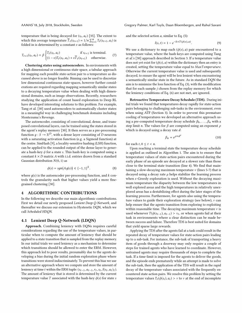
Algorithm 1 Application of temperature decay schedule (TDS)

1: Upon reaching a terminal state do2: n ← 0, steps ← steps taken during the episode3: for i = steps to 0 do4: if βnTt (ϕ(si ),ai ) < νt then5: Tt+1(ϕ(si ),ai ) ← βnTt (ϕ(si ),ai )6: else7: Tt+1(ϕ(si ),ai ) ← νt8: end if9: n ← n + 110: end for11: ν ← µ ν

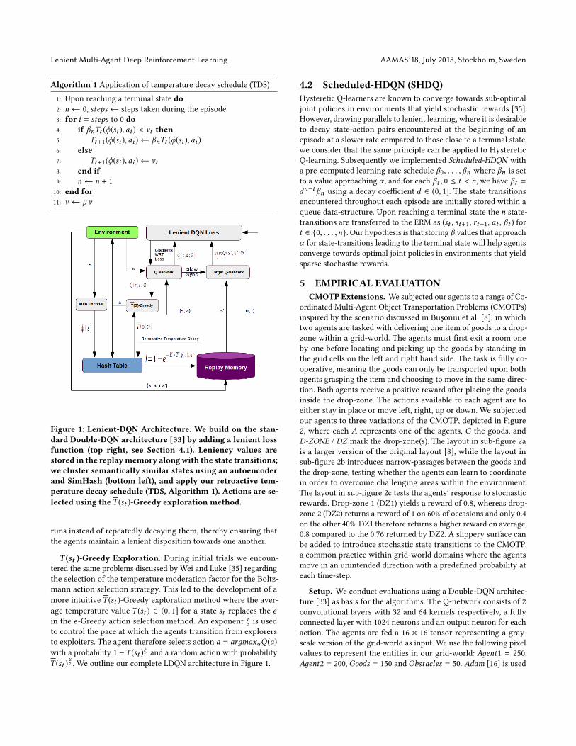
Figure 1: Lenient-DQN Architecture. We build on the stan-dard Double-DQN architecture [33] by adding a lenient lossfunction (top right, see Section 4.1). Leniency values arestored in the replaymemory alongwith the state transitions;we cluster semantically similar states using an autoencoderand SimHash (bottom left), and apply our retroactive tem-perature decay schedule (TDS, Algorithm 1). Actions are se-lected using the T (st )-Greedy exploration method.

runs instead of repeatedly decaying them, thereby ensuring thatthe agents maintain a lenient disposition towards one another.

T (st )-Greedy Exploration. During initial trials we encoun-tered the same problems discussed by Wei and Luke [35] regardingthe selection of the temperature moderation factor for the Boltz-mann action selection strategy. This led to the development of amore intuitive T (st )-Greedy exploration method where the aver-age temperature value T (st ) ∈ (0, 1] for a state st replaces the ϵin the ϵ-Greedy action selection method. An exponent ξ is usedto control the pace at which the agents transition from explorersto exploiters. The agent therefore selects action a = arдmaxaQ(a)with a probability 1 −T (st )ξ and a random action with probabilityT (st )ξ . We outline our complete LDQN architecture in Figure 1.

4.2 Scheduled-HDQN (SHDQ)Hysteretic Q-learners are known to converge towards sub-optimaljoint policies in environments that yield stochastic rewards [35].However, drawing parallels to lenient learning, where it is desirableto decay state-action pairs encountered at the beginning of anepisode at a slower rate compared to those close to a terminal state,we consider that the same principle can be applied to HystereticQ-learning. Subsequently we implemented Scheduled-HDQN witha pre-computed learning rate schedule β0, . . . , βn where βn is setto a value approaching α , and for each βt , 0 ≤ t < n, we have βt =dn−t βn using a decay coefficient d ∈ (0, 1]. The state transitionsencountered throughout each episode are initially stored within aqueue data-structure. Upon reaching a terminal state the n state-transitions are transferred to the ERM as (st , st+1, rt+1, at , βt ) fort ∈ {0, . . . ,n}. Our hypothesis is that storing β values that approachα for state-transitions leading to the terminal state will help agentsconverge towards optimal joint policies in environments that yieldsparse stochastic rewards.

5 EMPIRICAL EVALUATIONCMOTP Extensions. We subjected our agents to a range of Co-

ordinated Multi-Agent Object Transportation Problems (CMOTPs)inspired by the scenario discussed in Buşoniu et al. [8], in whichtwo agents are tasked with delivering one item of goods to a drop-zone within a grid-world. The agents must first exit a room oneby one before locating and picking up the goods by standing inthe grid cells on the left and right hand side. The task is fully co-operative, meaning the goods can only be transported upon bothagents grasping the item and choosing to move in the same direc-tion. Both agents receive a positive reward after placing the goodsinside the drop-zone. The actions available to each agent are toeither stay in place or move left, right, up or down. We subjectedour agents to three variations of the CMOTP, depicted in Figure2, where each A represents one of the agents, G the goods, andD-ZONE / DZ mark the drop-zone(s). The layout in sub-figure 2ais a larger version of the original layout [8], while the layout insub-figure 2b introduces narrow-passages between the goods andthe drop-zone, testing whether the agents can learn to coordinatein order to overcome challenging areas within the environment.The layout in sub-figure 2c tests the agents’ response to stochasticrewards. Drop-zone 1 (DZ1) yields a reward of 0.8, whereas drop-zone 2 (DZ2) returns a reward of 1 on 60% of occasions and only 0.4on the other 40%. DZ1 therefore returns a higher reward on average,0.8 compared to the 0.76 returned by DZ2. A slippery surface canbe added to introduce stochastic state transitions to the CMOTP,a common practice within grid-world domains where the agentsmove in an unintended direction with a predefined probability ateach time-step.

Setup. We conduct evaluations using a Double-DQN architec-ture [33] as basis for the algorithms. The Q-network consists of 2convolutional layers with 32 and 64 kernels respectively, a fullyconnected layer with 1024 neurons and an output neuron for eachaction. The agents are fed a 16 × 16 tensor representing a gray-scale version of the grid-world as input. We use the following pixelvalues to represent the entities in our grid-world: Aдent1 = 250,Aдent2 = 200, Goods = 150 and Obstacles = 50. Adam [16] is used

AAMAS’18, July 2018, Stockholm, Sweden Gregory Palmer, Karl Tuyls, Daan Bloembergen, and Rahul Savani

(a) Original (b) Narrow-Passage (c) Stochastic

Figure 2: CMOTP Layouts

to optimize the networks. Our initial experiments are conductedwithin a noise free environment, enabling us to speed up the testingof our LDQN algorithm without having to use an autoencoder forhashing; instead we apply python’s xxhash. We subsequently testthe LDQN with the autoencoder for hashing in a noisy versionof the stochastic reward CMOTP. The autoencoder consists of 2convolutional Layers with 32 and 64 kernels respectively, 3 fullyconnected layers with 1024, 512, and 1024 neurons followed by 2transposed convolutional layers. For our Scheduled-HDQN agentswe pre-compute β0 to n by setting βn = 0.9 and applying a decaycoefficient of d = 0.99 at each step t = 1 to n, i.e. βn−t = 0.99t βn ,with βn−t being bounded below at 0.4.We summarize the remaininghyper-parameters in Table 1. In Section 7 we include an extensiveanalysis of tuning the leniency related hyper-parameters. We noteat this point that each algorithm used the same learning rate αspecified in Table 1.

Component Hyper-parameter Setting

DQN-Optimization

Learning rate α 0.0001Discount rate γ 0.95

Steps between target network synchronization 5000ERM Size 250’000

ϵ -Greedy ExplorationInitial ϵ value 1.0ϵ Decay factor 0.999

Minimum ϵ Value 0.05

Leniency

MaxTemperature 1.0Temperature Modification Coefficient K 2.0

TDS Exponent ρ -0.01TDS Exponent Decay Rate d 0.95

Initial Max Temperature Value ν 1.0Max Temperature Decay Coefficient µ 0.999

Autoencoder HashKey Dimensions k 64Number of sigmoidal units in the dense layer D 512

Table 1: Hyper-parameters

6 DETERMINISTIC CMOTP RESULTSOriginal CMOTP. The CMOTP represents a challenging fully

cooperative task for parallel learners. Past research has shown thatdeep reinforcement learning agents can converge towards coop-erative policies in domains where the agents receive feedback fortheir individual actions, such as when learning to play pong withthe goal of keeping the ball in play for as long as possible [28].However, in the CMOTP feedback is only received upon deliveringthe goods after a long series of coordinated actions. No immediatefeedback is available upon miscoordination. When using uniformaction selection the agents only have a 20% chance of choosing

identical actions per state transition. As a result thousands of statetransitions are often required to deliver the goods and receive a re-ward while the agents explore the environment, preventing the useof a small replay memory where outdated transitions would be over-written within reasonable time. As a result standard Double-DQNarchitectures struggled to master the CMOTP, failing to coordinateon a significant number of runs even when confronted with therelatively simple original CMOTP.

We conducted 30 training runs of 5000 episodes per run for eachLDQN and HDQN configuration. Lenient and hysteretic agentswith β < 0.8 fared significantly better than the standard Double-DQN, converging towards joint policies that were only a few stepsshy of the optimal 33 steps required to solve the task. Lenientagents implemented with both ATF and TDS delivered a compara-ble performance to the hysteretic agents with regards to the averagesteps per episode and the coordinated steps percentage measuredover the final 100 steps of each episode (Table 2, left). However,both LDQN-ATF and LDQN-TDS averaged a statistically significanthigher number of steps per training run compared to hystereticagents with β < 0.7. For the hysteretic agents we observe a sta-tistically significant increase in the average steps per run as thevalues for β increase, while the average steps and coordinated stepspercentage over the final 100 episodes remain comparable.

Narrow Passage CMOTP. Lenient agents implemented withATF struggle significantly within the narrow-passage CMOTP, asevident from the results listed in Table 2 (right). We find that the av-erage temperature values cool off rapidly over the first 100 episodeswithin the Pickup and Middle compartments, as illustrated in Fig-ure 3. Meanwhile agents using TDS manage to maintain sufficientleniency over the first 1000 episodes to allow rewards to propagatebackwards from the terminal state. We conducted ATF experimentswith a range of values for the fold-in constant υ (0.2, 0.4 and 0.8),but always witnessed the same outcome. Slowing down the temper-ature decay would help agents using ATF remain lenient for longer,with the side-effects of an overoptimistic disposition in stochasticenvironments, and an increase in the number of steps required forconvergence if the temperatures are tied to the action selectionpolicy. Using TDS meanwhile allows agents to maintain sufficientleniency around difficult sub-tasks within the environment whilebeing able to decay later transitions at a faster rate. As a resultagents using TDS can learn the average rewards for state transi-tions close to the terminal state while remaining optimistic forupdates to earlier transitions.

Figure 3: Average temperature per compartment

Lenient Multi-Agent Deep Reinforcement Learning AAMAS’18, July 2018, Stockholm, Sweden

Original CMOTP Results Narrow-Passage CMOTP ResultsHyst. β = 0.5 Hyst. β = 0.6 Hyst. β = 0.7 Hyst. β = 0.8 LDQN ATF LDQN TDS Hyst. β = 0.5 Hyst. β = 0.6 LDQN ATF LDQN TDS

SPE 36.4 36.1 36.8 528.9 36.9 36.8 45.25 704.9 376.2 45.7CSP 92% 92% 92% 91% 92% 92% 92% 89% 90% 92%SPR 1’085’982 1’148’652 1’408’690 3’495’657 1’409’720 1’364’029 1’594’968 4’736’936 3’950’670 2’104’637

Table 2: Deterministic CMTOP Results, including average steps per episode (SPE) over the final 100 episodes, coordinatedsteps percentages (CSP) over the final 100 episodes, and the average steps per training run (SPR).

The success of HDQN agents within the narrow-passage CMOTPdepends on the value chosen for β . Agents with β > 0.5 struggle tocoordinate, as we observed over a large range of β values, exem-plars of which are given in Table 2. The only agents that convergeupon a near optimal joint-policy are those using LDQN-TDS andHDQN (β = 0.5). We performed a Kolmogorov-Smirnov test witha null hypothesis that there is no significant difference betweenthe performance metrics for agents using LDQN-TDS and HDQN(β = 0.5). We fail to reject the null hypothesis for average stepsper episode and percentage of coordinated steps for the final 100episodes. However, HDQN (β = 0.5) averaged significantly lesssteps per run while maintaining less overhead, replicating previousobservations regarding the strengths of hysteretic agents withindeterministic environments.

7 STOCHASTIC CMOTP RESULTSIn the stochastic setting we are interested in the percentage of runsfor each algorithm that converge upon the optimal joint policy,which is for the agents to deliver the goods to dropzone 1, yieldinga reward of 0.8, as opposed to dropzone 2 which only returns anaverage reward of 0.76 (see Section 5). We conducted 40 runs of5000 episodes for each algorithm.

As discussed in Section 6, HDQN agents using β > 0.7 frequentlyfail to coordinate in the deterministic CMOTP. Therefore, settingβ = 0.7 is the most likely candidate to succeed at solving the sto-chastic reward CMOTP for standard HDQN architectures. However,agents using HDQN (β = 0.7) only converged towards the optimalpolicy on 42.5% of runs. The scheduled-HDQN performed signifi-cantly better achieving a 77.5% optimal policy rate. Furthermorethe SHDQN performs well when an additional funnel-like narrow-passage is inserted close to the dropzones, with 93% success rate.The drop in performance upon removing the funnel suggests thatthe agents are led astray by the optimism applied to earlier tran-sitions within each episode, presumably around the pickup areawhere a crucial decision is made regarding the direction in whichthe goods should be transported.

LDQNusing ϵ−Greedy exploration performed similar to SHDQN,converging towards the optimal joint policy on 75% of runs. Mean-while LDQNs using T (st )-Greedy exploration achieved the highestpercentages of optimal joint-policies, with agents converging on100% of runs for the following configuration: K = 3.0, d = 0.9,ξ = 0.25 and µ = 0.9995, which will be discussed in more detailbelow. However the percentage of successful runs is related to thechoice of hyperparameters. We therefore include an analysis ofthree critical hyperparameters:• The temperature Modification CoefficientK , that determinesthe speed at which agents transition from optimist to averagereward learner (sub-figure 4a). Values: 1, 2 and 3

• The TDS decay-rate d which controls the rate at which tem-peratures are decayed n-steps prior to the terminal state(sub-figure 4b). Values: 0.9, 0.95 and 0.99• T (st )-Greedy exploration exponent ξ , controlling the agent’stransition from explorer to exploiter, with lower values forξ encouraging exploration. Values: 0.25, 0.5 and 1.0

(a) Leniency Schedules (b) TDS

Figure 4: TMC and TDS schedules used during analysis.

We conducted 40 simulation runs for each combination of thethree variables. To determine howwell agents using LDQN can copewith stochastic state transitions we added a slippery surface whereeach action results in a random transition with 10% probability1. The highest performing agents used a steep temperature decayschedule that maintains high temperatures for early transitions(d = 0.9 or d = 0.95) with temperature modification coefficientsthat slow down the transition from optimist to average rewardlearner (K = 2 or k = 3), and exploration exponents that delaythe transition from explorer to exploiter (ξ = 0.25 or ξ = 0.5).This is illustrated in the heat-maps in Figure 5. When using a TDSwith a more gradual incline (d = 0.99) the temperature values fromearlier state transitions decay at a similar rate to those near terminalstates. In this setting choosing larger values for K increases thelikelihood of the agents converging upon a sub-optimal policy priorto having established the average rewards available in later states,as evident from the results plotted in sub-figure 5c. Even whensetting the exploration exponent ξ to 0.25 the agents prematurelytransition to exploiter while holding an overoptimistic dispositiontowards follow-on states. Interestingly when K < 3 agents oftenconverge towards the optimal joint-policy despite setting d = 0.99.However, the highest percentages of optimal runs (97.5%) wereachieved through combining a steep TDS (d = 0.9 or d = 0.95) withthe slow transition to average reward learner (k = 3) and exploiter(ξ = 0.25). Meanwhile the lowest percentages for all TDSs resultedfrom insufficient leniency (K = 1) and exploration (ξ = 1.0).

Using one of the best-performing configuration (K = 3.0, d = 0.9and ξ = 0.25) we conducted further trials analyzing the agents’1Comparable results were obtained during preliminary trials without a slippery surface.

AAMAS’18, July 2018, Stockholm, Sweden Gregory Palmer, Karl Tuyls, Daan Bloembergen, and Rahul Savani

(a) d = 0.9 (b) d = 0.95 (c) d = 0.99

Figure 5: Analysis of the LDQN hyperparameters. Theheat-maps show the percentage of runs that converged to

the optimal joint-policy (darker is better).

sensitivity to the maximum temperature decay coefficient µ. Weconducted an additional set of 40 runs where µ was increased from0.999 to 0.9995. Combining T (S)-Greedy with the slow decayingµ = 0.9995 results in the agents spending more time exploring theenvironment at the cost of requiring longer to converge, resultingin an additional 1’674’106 steps on average per run. However, theagents delivered the best performance, converging towards theoptimal policy on 100% runs conducted.

Continuous State Space Analysis. Finally we show that se-mantically similar state-action pairs can be mapped to temperaturevalues using SimHash in conjunction with an autoencoder. We con-ducted experiments in a noisy version of the stochastic CMTOP,where at each time step every pixel value is multiplied by a uniquecoefficient drawn from a Gaussian distribution X ∼ N(1.0, 0.01).A non-sparse tensor is used to represent the environment, withbackground cells set to 1.0 prior to noise being applied.

Agents using LDQNs with xxhash converged towards the sub-optimal joint policy after the addition of noise as illustrated inFigure 6, with the temperature values decaying uniformly in tunewith ν . LDQN-TDS agents using an autoencoder meanwhile con-verged towards the optimal policy on 97.5% of runs. It is worthpointing out that the autoencoder introduces a new set of hyper-parameters that require consideration, including the size D of thedense layer at the centre of the autoencoder and the dimensionsK of the hash-key, raising questions regarding the influence of thegranularity on the convergence. We leave this for future work.

Figure 6: Noisy Stochastic CMOTP Average Reward

8 DISCUSSION & CONCLUSIONOur work demonstrates that leniency can help MA-DRL agentssolve a challenging fully cooperative CMOTP using high-dimensionaland noisy images as observations. Having successfully mergedleniency with a Double-DQN architecture raises the question re-garding how well our LDQN will work with other state of the artcomponents. We have recently conducted preliminary stochasticreward CMOTP trials with agents using LDQN with a PrioritizedExperience Replay Memory [1]. Interestingly the agents consistentlyconverged towards the sub-optimal joint policy. We plan to investi-gate this further in future work. In addition our research raises thequestion how well our extensions would perform in environmentswhere agents receive stochastic rewards throughout the episode. Toanswer this question we plan to test our LDQNwithin a hunter preyscenario where each episode runs for a fixed number of time-steps,with the prey being re-inserted at a random position each time itis caught [20]. Furthermore we plan to investigate how our LDQNresponds to environments with more than two agent by conductingCMOTP and hunter-prey scenarios with four agents.

To summarize our contributions:1) In this work we have shown that leniency can be applied toMA-DRL, enabling agents to converge upon optimal joint policieswithin fully-cooperative environments that require implicit coordi-nation strategies and yield stochastic rewards.2) We find that LDQNs significantly outperform standard andscheduled-HDQNs within environments that yield stochastic re-wards, replicating findings from tabular settings [35].3)We introduced two extensions to leniency, including a retroac-tive temperature decay schedule that prevents the premature decayof temperatures for state-action pairs and a T (st )-Greedy explo-ration strategy that encourages agents to remain exploratory instates with a high average temperature value. The extensions canin theory also be used by lenient agents within non-deep settings.4) Our LDQN hyperparameter analysis revealed that the highestperforming agents within stochastic reward domains use a steeptemperature decay schedule that maintains high temperatures forearly transitions combined with a temperature modification coef-ficient that slows down the transition from optimist to averagereward learner, and an exploration exponent that delays the transi-tion from explorer to exploiter.5)We demonstrate that the CMOTP [8] can be used as a benchmark-ing environment for MA-DRL, requiring reinforcement learningagents to learn fully-cooperative joint-policies from processinghigh dimensional and noisy image observations.6) Finally, we introduce two extensions to the CMOTP. First weinclude narrow passages, allowing us to test lenient agents’ abil-ity to prevent the premature decay of temperature values. Oursecond extension introduces two dropzones that yield stochasticrewards, testing the agents’ ability to converge towards an optimaljoint-policy while receiving misleading rewards.

9 ACKNOWLEDGMENTSWe thank the HAL Allergy Group for partially funding the PhD ofGregory Palmer and gratefully acknowledge the support of NVIDIACorporation with the donation of the Titan X Pascal GPU thatenabled this research.

Lenient Multi-Agent Deep Reinforcement Learning AAMAS’18, July 2018, Stockholm, Sweden

REFERENCES[1] Ioannis Antonoglou, John Quan Tom Schaul, and David Silver. 2015. Prioritized

Experience Replay. arXiv preprint arXiv:1511.05952 (2015).[2] Tucker Balch and Ronald C Arkin. 1994. Communication in reactive multiagent

robotic systems. Autonomous robots 1, 1 (1994), 27–52.[3] Nikos Barbalios and Panagiotis Tzionas. 2014. A robust approach for multi-agent

natural resource allocation based on stochastic optimization algorithms. AppliedSoft Computing 18 (2014), 12–24.

[4] Andrew Barto and Richard Sutton. 1998. Reinforcement learning: An introduction.MIT press.

[5] Daan Bloembergen, Daniel Hennes, Michael Kaisers, and Karl Tuyls. 2015. Evo-lutionary dynamics of multi-agent learning: A survey. Journal of Artificial Intelli-gence Research 53 (2015), 659–697.

[6] Daan Bloembergen, Michael Kaisers, and Karl Tuyls. 2011. Empirical and the-oretical support for lenient learning. In The 10th International Conference onAutonomous Agents and Multiagent Systems-Volume 3. International Foundationfor Autonomous Agents and Multiagent Systems, 1105–1106.

[7] Lucian Busoniu, Robert Babuska, and Bart De Schutter. 2008. A comprehensivesurvey of multiagent reinforcement learning. IEEE Transactions on Systems, Man,And Cybernetics-Part C: Applications and Reviews, 38 (2), 2008 (2008).

[8] Lucian Buşoniu, Robert Babuška, and Bart De Schutter. 2010. Multi-agent re-inforcement learning: An overview. In Innovations in multi-agent systems andapplications-1. Springer, 183–221.

[9] Moses S Charikar. 2002. Similarity estimation techniques from rounding algo-rithms. In Proceedings of the thiry-fourth annual ACM symposium on Theory ofcomputing. ACM, 380–388.

[10] Tim de Bruin, Jens Kober, Karl Tuyls, and Robert Babuška. 2015. The importanceof experience replay database composition in deep reinforcement learning. InDeep Reinforcement Learning Workshop, NIPS.

[11] Jakob Foerster, Nantas Nardelli, Gregory Farquhar, Philip Torr, Pushmeet Kohli,ShimonWhiteson, et al. 2017. Stabilising Experience Replay for DeepMulti-AgentReinforcement Learning. arXiv preprint arXiv:1702.08887 (2017).

[12] Shixiang Gu, Ethan Holly, Timothy Lillicrap, and Sergey Levine. 2016. DeepReinforcement Learning for Robotic Manipulation with Asynchronous Off-PolicyUpdates. arXiv preprint arXiv:1610.00633 (2016).

[13] Jayesh K Gupta, Maxim Egorov, and Mykel Kochenderfer. 2017. CooperativeMulti-Agent Control Using Deep Reinforcement Learning. In Proceedings of theAdaptive and Learning Agents workshop (at AAMAS 2017).

[14] Pablo Hernandez-Leal, Michael Kaisers, Tim Baarslag, and Enrique Munoz deCote. 2017. A Survey of Learning in Multiagent Environments: Dealing withNon-Stationarity. arXiv preprint arXiv:1707.09183 (2017).

[15] Leslie Pack Kaelbling, Michael L Littman, and Andrew W Moore. 1996. Rein-forcement learning: A survey. Journal of artificial intelligence research 4 (1996),237–285.

[16] Diederik P. Kingma and JimmyBa. 2014. Adam: AMethod for Stochastic Optimiza-tion. In Proceedings of the 3rd International Conference on Learning Representations(ICLR).

[17] Guillaume Lample and Devendra Singh Chaplot. 2017. Playing FPS Games withDeep Reinforcement Learning. AAAI (2017), 2140–2146.

[18] Long-H Lin. 1992. Self-improving reactive agents based on reinforcement learn-ing, planning and teaching. Machine learning 8, 3/4 (1992), 69–97.

[19] Laëtitia Matignon, Guillaume J Laurent, and Nadine Le Fort-Piat. 2007. Hystereticq-learning: an algorithm for decentralized reinforcement learning in cooperativemulti-agent teams. In Intelligent Robots and Systems, 2007. IROS 2007. IEEE/RSJInternational Conference on. IEEE, 64–69.

[20] Laetitia Matignon, Guillaume J Laurent, and Nadine Le Fort-Piat. 2012. Indepen-dent reinforcement learners in cooperative Markov games: a survey regardingcoordination problems. The Knowledge Engineering Review 27, 1 (2012), 1–31.

[21] Volodymyr Mnih, Koray Kavukcuoglu, David Silver, Andrei A Rusu, Joel Veness,Marc G Bellemare, Alex Graves, Martin Riedmiller, Andreas K Fidjeland, GeorgOstrovski, et al. 2015. Human-level control through deep reinforcement learning.Nature 518, 7540 (2015), 529–533.

[22] Shayegan Omidshafiei, Jason Pazis, Christopher Amato, Jonathan P How, andJohn Vian. 2017. Deep decentralized multi-task multi-agent reinforcement learn-ing under partial observability. In International Conference on Machine Learning.2681–2690.

[23] Liviu Panait, Keith Sullivan, and Sean Luke. 2006. Lenient learners in cooperativemultiagent systems. In Proceedings of the fifth international joint conference onAutonomous agents and multiagent systems. ACM, 801–803.

[24] Liviu Panait, Karl Tuyls, and Sean Luke. 2008. Theoretical advantages of le-nient learners: An evolutionary game theoretic perspective. Journal of MachineLearning Research 9, Mar (2008), 423–457.

[25] Mitchell A Potter and Kenneth A De Jong. 1994. A cooperative coevolutionaryapproach to function optimization. In International Conference on Parallel ProblemSolving from Nature. Springer, 249–257.

[26] Tom Schaul, John Quan, Ioannis Antonoglou, and David Silver. 2015. Prioritizedexperience replay. arXiv preprint arXiv:1511.05952 (2015).

[27] Peter Sunehag, Guy Lever, Audrunas Gruslys, Wojciech Marian Czarnecki, Vini-cius Zambaldi, Max Jaderberg, Marc Lanctot, Nicolas Sonnerat, Joel Z Leibo, KarlTuyls, and Thore Graepel. 2017. Value-Decomposition Networks For CooperativeMulti-Agent Learning. arXiv preprint arXiv:1706.05296 (2017).

[28] Ardi Tampuu, Tambet Matiisen, Dorian Kodelja, Ilya Kuzovkin, Kristjan Kor-jus, Juhan Aru, Jaan Aru, and Raul Vicente. 2017. Multiagent cooperation andcompetition with deep reinforcement learning. PLoS One 12, 4 (2017), e0172395.

[29] Ming Tan. 1993. Multi-agent reinforcement learning: Independent vs. cooperativeagents. In Proceedings of the tenth international conference on machine learning.330–337.

[30] Haoran Tang, Rein Houthooft, Davis Foote, Adam Stooke, Xi Chen, Yan Duan,John Schulman, Filip De Turck, and Pieter Abbeel. 2016. # Exploration: A Studyof Count-Based Exploration for Deep Reinforcement Learning. arXiv preprintarXiv:1611.04717 (2016).

[31] Karl Tuyls and Gerhard Weiss. 2012. Multiagent Learning: Basics, Challenges,and Prospects. AI Magazine 33, 3 (2012), 41–52.

[32] Hado Van Hasselt. 2010. Double Q-learning. In Advances in Neural InformationProcessing Systems. 2613–2621.

[33] Hado Van Hasselt, Arthur Guez, and David Silver. 2016. Deep ReinforcementLearning with Double Q-Learning. AAAI (2016), 2094–2100.

[34] Christopher JCH Watkins and Peter Dayan. 1992. Q-learning. Machine learning8, 3-4 (1992), 279–292.

[35] Ermo Wei and Sean Luke. 2016. Lenient Learning in Independent-Learner Sto-chastic Cooperative Games. Journal of Machine Learning Research 17, 84 (2016),1–42. http://jmlr.org/papers/v17/15-417.html

[36] R Paul Wiegand. 2003. An analysis of cooperative coevolutionary algorithms. Ph.D.Dissertation. George Mason University Virginia.

[37] Yinliang Xu, Wei Zhang, Wenxin Liu, and Frank Ferrese. 2012. Multiagent-basedreinforcement learning for optimal reactive power dispatch. IEEE Transactionson Systems, Man, and Cybernetics, Part C (Applications and Reviews) 42, 6 (2012),1742–1751.