Lecture5a Consumer Choice Examples
7
5a Consumer Choice Examples Optimization and Human Behavior Handout for Managerial Economics October 21, 2011 Thomas F. Rutherford, Center for Energy Policy and Economics, ETH Zürich 5a.1 A Choice Experiment Thomas lives in Ann Arbor where he currently spends 30% of his income on rent. He has an employment offer in Zürich which pays 50% more than he currently earns, but he is hesitant to take the job because rental rates in Zürich are three times higher than in Ann Arbor. Assum- ing that Thomas has CES preferences with elasticity of substitution σ ; on purely economic grounds, should he move? As is the case for all interesting questions in economics, the only good answer to this problem is “It depends.”. 5a.2 Intuition Thomas’s offer in Zürich does not pay him enough to live exactly the lifestyle that he enjoys in Ann Arbor, as he would need a 60% raise to cover rent and consumption. The elasticity of substitution is key. If it is high, he more willing substitutes consumption of goods and services for housing and thereby lowers his cost of living in Zürich. On the other hand, if the elas ticit y is low, he is “stuck in his ways” , and the move is a bad idea. 5a.3 Calibration to a Benchmark Equilibrium We are given information about Thomas’s choices in Ann Arbor. This information is essentially an observation of a benchmark equilibrium, consisting of the prevai ling prices and quantities of goods demand. The benchmark equilibrium data together with assumptions about elasticities are used to evaluate Thomas’s choices after a discr ete change in the economic enviro nmen t. The steps invo lved in solvi ng this little textbook model are identical to those typically employed in applied general equilibrium analysis. 5a.4 Graphical Representation 5a.5 1
Transcript of Lecture5a Consumer Choice Examples

8/13/2019 Lecture5a Consumer Choice Examples
http://slidepdf.com/reader/full/lecture5a-consumer-choice-examples 1/7
5aConsumer Choice ExamplesOptimization and Human Behavior
Handout for Managerial Economics October 21, 2011
Thomas F. Rutherford, Center for Energy Policy and Economics, ETH Zürich
5a.1
A Choice Experiment
Thomas lives in Ann Arbor where he currently spends 30% of his income on rent. He has an
employment offer in Zürich which pays 50% more than he currently earns, but he is hesitant
to take the job because rental rates in Zürich are three times higher than in Ann Arbor. Assum-
ing that Thomas has CES preferences with elasticity of substitution σ ; on purely economic
grounds, should he move?
As is the case for all interesting questions in economics, the only good answer to this problem is “It
depends.”. 5a.2
Intuition
Thomas’s offer in Zürich does not pay him enough to live exactly the lifestyle that he enjoys in Ann
Arbor, as he would need a 60% raise to cover rent and consumption. The elasticity of substitution is key.
If it is high, he more willing substitutes consumption of goods and services for housing and thereby lowers
his cost of living in Zürich. On the other hand, if the elasticity is low, he is “stuck in his ways”, and the
move is a bad idea. 5a.3
Calibration to a Benchmark Equilibrium
We are given information about Thomas’s choices in Ann Arbor. This information is essentially anobservation of a benchmark equilibrium, consisting of the prevailing prices and quantities of goods demand.
The benchmark equilibrium data together with assumptions about elasticities are used to evaluate Thomas’s
choices after a discrete change in the economic environment. The steps involved in solving this little
textbook model are identical to those typically employed in applied general equilibrium analysis. 5a.4
Graphical Representation
5a.5
1

8/13/2019 Lecture5a Consumer Choice Examples
http://slidepdf.com/reader/full/lecture5a-consumer-choice-examples 2/7
Preferences
The utility function:
U (C , H ) = (α C ρ + (1−α ) H ρ)1/ρ
Exponent ρ is defined by the elasticity of substitution, σ , as
ρ = 1−1/σ .
The model of consumer choice is:
maxU (C , H ) s.t. C + p H H = M
5a.6
Demand
Derivation of demand functions which solve the utility maximization problem involves solving two
equations in two unknowns:
∂ U /∂ H
∂ U /∂ C =
(1−α ) H ρ−1
α C ρ−1 = p H ;
hence H
C =
1−α
α p H
σ
Substituting into the budget constraint, we have:
H = M
p H +α p H
1−α
σ = (1−α )σ M p−σ H
α σ + (1−α )σ p1−σ H
and
C = M
1 + p H
1−α α p H
σ = α σ M
α σ + (1−α )σ p1−σ H
5a.7
Calibration
It is conventional in applied general equilibrium analysis to employ exogenous elasticities and calibrated
value values. If we follow this approach, σ is then exogenous and α is calibrated.
Choosing units so that the benchmark price of housing ( ¯ p H ) is unity, we have:
θ = ¯ p H ¯ H / ¯ M
Substitute into the demand function:
1 +
α
1−α
σ
=¯ M
¯ H =
1
θ ;
and then solve for the preference parameter α :
α = (1−θ )1/σ
θ 1/σ + (1−θ )1/σ .
5a.8
Money Metric Utility
Substitute for α in U (C , H ), and denoting the base year expenditure on other goods as C = (1−θ ) ¯ M ,we have
U (C , H ) = κ
(1−θ )1/σ C ρ +θ 1/σ H ρ1/ρ
where the κ is a constant which may take on any positive value without altering the preference ordering.
It is convenient to assign this value to the benchmark expenditure, so that utility can be measured in money-
metric units at benchmark prices.
Noting that θ 1/σ = θ 1−ρ , we then can write the utility function as:
U (C , H ) = ¯ M
(1−θ )
C
C
ρ
+θ
H
¯ H
ρ1/ρ
5a.9
2

8/13/2019 Lecture5a Consumer Choice Examples
http://slidepdf.com/reader/full/lecture5a-consumer-choice-examples 3/7
Indirect Utility
Formally, we have:
V ( p H , M ) = U (C ( p H , M ), M ( p H , M )) = M
α σ + (1−α )σ p1−σ H
1/(1−σ )
In money-metric terms, we can use benchmark income to normalize the utility function:
V ( p H , M ) = M
(1−
θ + θ p
1−σ
H )1/(1−σ )
5a.10
Demand Functions – Calibrated Share Form
H = ¯ H V ( p H , M )
¯ M
pU
p H
σ
C = C V ( p H , M )
¯ M
pU
1
σ where
pU =
1−θ + θ p1−σ H
1/(1−σ )
5a.11
Should Thomas Move?Thomas’s welfare level in Zürich can be easily computed in money-metric terms as:
V ( p H = 3, M = 1.5) = 1.5
0.7 + 0.3×31−σ 1/(1−σ )
This expression cannot (to my knowledge) be solved in closed form, however it is easily to solve using
Excel. The critical value for σ is that which equates welfare in Zürich with welfare level in Ann Arbor, i.e.
V = 1. The numerical value is found to be σ ∗ = 0.441. The general dependence of welfare on the θ and σ can be illustrated in a contour diagram. 5a.12
Dependence of Welfare on Benchmark Shares and Elasticity
5a.13
Multivariable OptimizationThe concept of multivariate optimization is important in managerial economics because many demand
and supply relations involve more than two variables. In demand analysis, it is typical to consider the
quantity sold as a function of the price of the product itself, the price of other goods, advertising, income,
and other factors. In cost analysis, cost is determined by output, input prices, the nature of technology, and
so on.. 5a.14
3

8/13/2019 Lecture5a Consumer Choice Examples
http://slidepdf.com/reader/full/lecture5a-consumer-choice-examples 4/7
Optimal Advertising
To explore the concepts of multivariate optimization and the optimal level of advertising, consider
a hypothetical multivariate product demand function for CSI, Inc., where the demand for product Q is
determined by the price charged, P, and the level of advertising, A:
Q = 5,000−10P + 40 A + PA−0.8 A2−0.5P2
Determine the joint optimal price (P∗) and level of advertising ( A∗) which maximize CSI output. 5a.15
First Order ConditionsBegin by calculating partial derivates of demand with respect to price and level of advertising:
∂ Q
∂ P= −10 + A−P
∂ Q
∂ A= 40 + P−1.6 A
First order conditions for maximization of demand are:
∂ Q
∂ P= 0
∂ Q
∂ A= 0
5a.16
Optimization = Solving Simultaneous Equations
Hence, the optimal level of price and advertising solve:
−10 + A−P = 0
40 + P−1.6 A = 0
Hence, P∗ = 40, A∗ = $5,000 and the maximal output is Q∗ = 5,800.
Note that in subsequent chapters we will learn that the policies which maximize output may differ from
those which maximal profit, depending on how production cost relates to output. 5a.17
Nonlinear Pricing
Consider a consumer choice model in which the two goods consist of telecommunication services ( x)and all other goods ( y). Let the price of other goods is fixed at unity. Telecommunication services are
somewhat special in that due to economies of scale, these are offered with potentially substantial quantity
discounts. Once a subscription fee of f CHF is made, services are offerred at a substantially reduced price.
In the absence of the connection fee, p x = 1. Telecommunication services made to customers who have
paid the connection fee are offered at a price of ˆ p x.
The consumer is assumed to have the following utility function:
maxU ( x, y) = xα y1−α
5a.18
A. Ignoring the subscription plan, solve for the quantity of telecommunication services demanded by
the consumer.
The standard consumer model is one of budget-constrained utility maximization. Hence, we solve
maxU ( x, y) s.t. p x x + y = M . The first order condition is:
∂ U ( x, y)/∂ x
∂ U ( x, y)/∂ y=
p x
1
Hence,
x∗ = α M
p x
and
y∗ = (1−α ) M
15a.19
4

8/13/2019 Lecture5a Consumer Choice Examples
http://slidepdf.com/reader/full/lecture5a-consumer-choice-examples 5/7
B. Assuming that the consumer chooses to buy a subscription. Show that she will buy the following
quantities:
ˆ x∗ = α M − f
ˆ p x
ˆ y∗ = (1−α )( M − f )
If the consumer buys a subscription, the purchase quantity solves:
maxU ( x, y)
s.t.
ˆ p x x + y = M − f .
The first order conditions are identical to the previous case, except that M is replaced by M − f and
p x is replaced by ˆ p x.5a.20
C. Holding ˆ p fixed, what is the critical value of f such that the consumer is indifferent about buying a
subscription.
The critical value of f is that for which:
U ( x∗, y∗) = U ( ˆ x∗, ˆ y∗)
Substituting for U () we have:α
M
p x
α (1−α )
M
1
1−α
=
α
M − f
ˆ p x
α (1−α )
M − f
1
1−α
Thus, M
pα x
= M − f
ˆ pα x
and
f ∗ = M
1−
ˆ p x
p x
α 5a.21
D. Sketch the budget constraint and the optimal choice for a consumer who chooses not to accept the
subscription.
If a consumer buys a subscription, the maximum amount she can purchase of other goods is M − f .The slope of the budget line is − ˆ p. If the optimal point on the subscription-based budget constraint
is associated with a lower indifference curve, then the consumer will not purchase a subscription:
5a.22
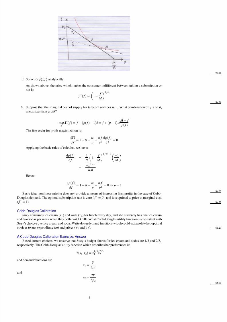
E. Holding f fixed, graphically find the maximum discount price level which would induce this con-
sumer to purchase additional units of telecommunication services ( ˆ p∗ x ).
Here we rotate the subscription based budget constraint around the y axis intercept to the point that it
is just tangent to the original indifference curve:
5
8/13/2019 Lecture5a Consumer Choice Examples
http://slidepdf.com/reader/full/lecture5a-consumer-choice-examples 6/7
5a.23
F. Solve for ˆ p∗h( f ) analytically.
As shown above, the price which makes the consumer indifferent between taking a subscription or
not is:
ˆ p∗( f ) =
1−
f
M
1/α
5a.24
G. Suppose that the marginal cost of supply for telecom services is 1. What combination of f and ˆ p x
maximizes firm profit?
max f Π( f ) = f + ( p( f )−1) ˆ x = f + ( p−1)α
M − f
p( f )
The first order for profit maximization is:
dΠ
d f = 1−α −
α
p−
α f
p2
d p( f )
d f = 0
Applying the basic rules of calculus, we have:
d p( f )
d f =
1
α
1−
f
M
1/α −1−1
M
=
− p1−α
α M
Hence:
d p( f )
d f = 1−α +
α
p+ α f
p2 = 0 ⇒ p = 1
5a.25Basic idea: nonlinear pricing does not provide a means of increasing firm profits in the case of Cobb-
Douglas demand. The optimal subscription rate is zero ( f ∗ = 0), and it is optimal to price at marginal cost
( ˆ p∗ = 1). 5a.26
Cobb-Douglas Calibration
Suzy consumes ice cream ( x1) and soda ( x2) for lunch every day, and she currently has one ice cream
and two sodas per week when they both cost 1 CHF. What Cobb-Douglas utility function is consistent with
Suzy’s choices over ice cream and soda. Write down demand functions which could extrapolate her optimal
choices to any expenditure (m) and prices ( p1 and p2). 5a.27
A Cobb-Douglas Calibration Exercise: Answer
Based current choices, we observe that Suzy’s budget shares for ice cream and sodas are 1/3 and 2/3,
respectively. The Cobb-Douglas utility function which describes her preferences is:
U ( x1, x2) = x1/31 x
2/32
and demand functions are
x1 = Y
3 p1
and
x2 = 2Y
3 p25a.28
6

8/13/2019 Lecture5a Consumer Choice Examples
http://slidepdf.com/reader/full/lecture5a-consumer-choice-examples 7/7
Calibration Exercise #2
Suppose that irregardless of relative prices, Suzy always has one soda before and one soda after eating
an ice cream. What utility function is consistent with these choices? Write down demand functions which
could extrapolate her optimal choices to any expenditure (m) and prices ( p1 and p2). 5a.29
Exercise # 2: Solution
Perfect complement preferences have the form:
U ( x1, x2) = min( x1
a1
, x2
a2
)
in which the ratio a1
a2determines the ratio in which goods 1 and 2 are consumed. In the present example,
we have:
U ( x1, x2) = min( x1, x2
2 )
and demand functions given by:
x1 = Y
p1 + 2 p2
and
x2 = 2 Y
p1 + 2 p25a.30
Calibration Exercise #3
When Suzy gets to the lunch counter, she always asks about the price of ice cream and the price of soda.If two sodas cost less than one ice cream, she has spends all of her money on soda. Otherwise she buys ice
cream. What utility function is consistent with these choices? Write down demand functions which could
extrapolate her optimal choices to any expenditure (m) and prices ( p1 and p2). 5a.31
Calibration Exercise #3 Solution
General perfect substitues preferences have the form:
U ( x1, x2) = a1 x1 + a2 x2
in which the ratio a1a2
represents the marginal rate of substitution of good 1 for good 2. The demand functions
for these preferences are given by:
x1 = 0 when p1
p2> a1
a2 M
p1 otherwise
x2 =
0 when p1
p2< a1
a2 M p2
otherwise5a.32
7