Lecture Notes for CAAM 378 A Quick Introduction to …yzhang/caam378/Notes/lec_notes.pdf · A Quick...

Lecture Notes for CAAM 378

A Quick Introduction to Linear Programming

(DRAFT)

Yin Zhang

Sept. 25, 2007

Contents

1 What is Linear Programming? 51.1 A Toy Problem . . . . . . . . . . . . . . . . . . . . . . . . . . 51.2 From Concrete to Abstract . . . . . . . . . . . . . . . . . . . . 61.3 A Standard Form . . . . . . . . . . . . . . . . . . . . . . . . . 81.4 Feasibility and Solution Sets . . . . . . . . . . . . . . . . . . . 101.5 Three Possibilities . . . . . . . . . . . . . . . . . . . . . . . . . 11

2 Vertices of the Feasibility Set 132.1 Matrix and Vector Partitions . . . . . . . . . . . . . . . . . . 132.2 Convex Set, Polyhedron and Extreme Point . . . . . . . . . . 15

2.2.1 Definitions . . . . . . . . . . . . . . . . . . . . . . . . . 152.2.2 Vertices of Feasibility Set . . . . . . . . . . . . . . . . . 162.2.3 Basic Feasible Partitions and Vertices . . . . . . . . . . 18

2.3 Exercises . . . . . . . . . . . . . . . . . . . . . . . . . . . . . . 19

3 Simplex Method: First Look 213.1 Terminology . . . . . . . . . . . . . . . . . . . . . . . . . . . . 213.2 Reduced Linear Program . . . . . . . . . . . . . . . . . . . . . 21

3.2.1 Partitioning and Elimination . . . . . . . . . . . . . . . 213.2.2 Reduced Linear Program . . . . . . . . . . . . . . . . . 223.2.3 What Happens at A Basic Feasible Solution? . . . . . . 23

3.3 One Iteration of the Simplex Method . . . . . . . . . . . . . . 243.4 Do We Reach a New Vertex? . . . . . . . . . . . . . . . . . . . 253.5 Exercises . . . . . . . . . . . . . . . . . . . . . . . . . . . . . . 26

4 Simplex Method: More Details 274.1 How to Start Simplex? – Two Phases . . . . . . . . . . . . . . 27

4.1.1 Phase-I: An Auxiliary Problem . . . . . . . . . . . . . 28

3

4 CONTENTS

4.1.2 Phase-II: The Original Problem . . . . . . . . . . . . . 294.2 Main Implemetational Issues . . . . . . . . . . . . . . . . . . . 304.3 Degeneracy, Cycling and Stalling . . . . . . . . . . . . . . . . 304.4 Exercises . . . . . . . . . . . . . . . . . . . . . . . . . . . . . . 30

5 Duality and Optimality Conditions 335.1 Dual Linear Program . . . . . . . . . . . . . . . . . . . . . . . 335.2 Optimality Conditions . . . . . . . . . . . . . . . . . . . . . . 355.3 How to find a dual? . . . . . . . . . . . . . . . . . . . . . . . . 355.4 Exercises . . . . . . . . . . . . . . . . . . . . . . . . . . . . . . 38

6 Primal-Dual Interior-Point Methods 396.1 Introduction . . . . . . . . . . . . . . . . . . . . . . . . . . . . 396.2 A Primal-Dual Method . . . . . . . . . . . . . . . . . . . . . . 406.3 Solving the Linear System . . . . . . . . . . . . . . . . . . . . 436.4 Convergence Considerations . . . . . . . . . . . . . . . . . . . 44

A Introduction to Newton’s Method 47A.1 An Example . . . . . . . . . . . . . . . . . . . . . . . . . . . . 50A.2 Exercises . . . . . . . . . . . . . . . . . . . . . . . . . . . . . . 51

Chapter 1

What is Linear Programming?

An optimization problem usually has three essential ingredients: a variablevector x consisting of a set of unknowns to be determined, an objectivefunction of x to be optimized, and a set of constraints to be satisfied by x.

A linear program is an optimization problem where all involved functionsare linear in x; in particular, all the constraints are linear inequalities andequalities. Linear programming is the subject of studying and solving linearprograms.

Linear programming was born during the second World War out of thenecessity of solving military logistic problems. It remains one of the mostused mathematical techniques in today’s modern societies.

1.1 A Toy Problem

A local furniture shop makes chairs and tables. The projected profits forthe two products are, respectively, $20 per chair and $30 per table. Theprojected demand is 400 chairs and 100 tables. Each chair requires 2 cubicfeet of wood while each table requires 4 cubic feet. The shop has a totalamount of 1,000 cubic feet of wood in stock. How many chairs and tablesshould the shop make in order to maximize its profit?

Let x1 be the number of chairs and x2 be the number of tables to be made.These are the two variables, or unknowns, for this problem. The shop wantsto maximize its total profit, 20x1 + 30x2, subject to the constraints that (a)the total amount of wood used to make the two products can not exceed the1,000 cubic feet available, and (b) the numbers of chairs and tables to be

5

6 CHAPTER 1. WHAT IS LINEAR PROGRAMMING?

made should not exceed the demands. In additional, we should not forgetthat the number of chairs and tables made need to be nonnegative. Puttingall these together, we have an optimization problem:

max 20x1 + 30x2s.t. 2x1 + 4x2 ≤ 1000

0 ≤ x1 ≤ 4000 ≤ x2 ≤ 100

(1.1)

where 20x1 + 30x2 is the objective function, “s.t.” is the shorthand for “sub-ject to” which is followed by the constraints of this problem.

This optimization problem is clearly a linear program where all the func-tions involved, both in the objective and in the constraints, are linear func-tions of x1 and x2.

1.2 From Concrete to Abstract

Let us look at an abstract production model. A company produces n prod-ucts using m kinds of materials. For the next month, the unit profits forthe n products are projected to be c1, c2, · · · , cn. The amounts of mate-rials available to the company in the next month are b1, b2, · · · , bm. Theamount of material i consumed by a unit of product j is given by aij ≥ 0 fori = 1, 2, · · · ,m and j = 1, 2, · · · , n (some aij could be zero if product j doesnot use material i). The question facing the company is, given the limitedavailability of materials, what quantity the company should produce in thenext month for each product in order to achieve the maximum total profit?

The decision variables are obviously the amounts produced for the nproducts in the next month. Let us call them x1, x2, · · · , xn. The optimiza-tion model is to maximize the total profit, subject to the material availabilityconstraints for all m materials, and the nonnegativity constraints on the nvariables.

In mathematical terms, the model is the following linear program:

1.2. FROM CONCRETE TO ABSTRACT 7

max c1x1 + c2x2 + · · ·+ cnxns.t. a11x1 + a12x2 + · · ·+ a1nxn ≤ b1

a21x1 + a22x2 + · · ·+ a2nxn ≤ b2...

am1x1 + am2x2 + · · ·+ amnxn ≤ bmx1, x2, · · · , xn ≥ 0

(1.2)

The nonnegativity constraints can be vital, but are often forgotten bybeginners. Why is nonnegativity important here? First, in the above context,it does not make sense to expect the company to produce a negative amountof a product. Moreover, if one product, say product k, is not profitable,corresponding to ck < 0, without the nonnegativity constraints the modelwould produce a solution xk < 0 and generate a profit ckxk > 0. In fact,since a negative amount of product k would not consume any material butinstead “generate” materials, one could drive the profit to infinity by forcingxk to go to negative infinity. Hence, the model would be wrong had oneforgotten nonnegativity.

The linear program in (1.2) is tedious to write. One can shorten theexpressions using the summation notation. For example, the total profit canbe represented by the left-hand side instead of the right-hand side of thefollowing identity

n∑i=1

cixi = c1x1 + c2x2 + · · ·+ cnxn.

However, a much more concise way is to use matrices and vectors. If welet c = (c1, c2, · · · , cn)T and x = (x1, x2, · · · , xn)T . Then the total profitbecomes cTx. In a matrix-vector notation, the linear program (1.2) becomes

max cTxs.t. Ax ≤ b

x ≥ 0(1.3)

where A ∈ <m×n and b ∈ <m. The inequalities involving vectors are alwaysunderstood as component-wise comparisons. For example, the n-vector x ≥ 0means that each component xi ≥ 0 for i = 1, 2, · · · , n.


1.3 A Standard Form

A linear program can have an objective of either minimization or maximiza-tion, while its constraints can have any combination of linear inequalitiesand equalities. It is impractical to study linear programs and to design algo-rithms for them without introducing a so-called standard form – a unifyingframework encompassing most, if not all, individual forms of linear programs.Different standard forms exist in the literature that may offer different advan-tages under different circumstances. Here we will use the following standardform:

min cTxs.t. Ax = b

x ≥ 0(1.4)

where the matrix A is m × n, b ∈ <m and c, x ∈ <n. The triple (A, b, c)represents problem data that needs to be specified, and x is the variable tobe determined. In fact, once the size of A is given, the sizes of all the otherquantities follow accordingly from the rule of matrix multiplication.

In plain English, a standard linear program is one that is a minimizationproblem with a set of equality constraints but no inequality constraints exceptnonnegativity on all variables.

We will always assume that A has full rank, or in other words, the rowsof A are linearly independent which ensures that the equations in Ax = bare consistent for any right-hand side b ∈ <m. We make this assumption tosimplify the matter without loss of generality, because redundant or inconsis-tent linear equations can always be detected, and removed through standardlinear algebra techniques. Moreover, we normally require that the matrix Ahave more columns than rows, that is m < n. This requirement, togetherwith the full rank of A, ensures that there are infinitely many solutions tothe equation Ax = b, leaving degrees of freedom for nonnegative and optimalsolutions.

A linear program is said to be equivalent to another linear program ifan optimal solution of the former, if it exists, can be obtained from an op-timal solution of the latter through some simple algebraic operations. Thisequivalence allows one to solve one and obtain a solution to the other.

We claim that every linear program is equivalent to a standard-form lin-ear program through a transformation, which usually requires adding extravariables and constraints. Obviously, maximizing a function is equivalent tominimizing the negative of the function. A common trick to transform an

1.3. A STANDARD FORM 9

inequality aTx ≤ β into an equivalent equality is to add a so-called slackvariable η so that

aTx ≤ β ⇐⇒ aTx+ η = β, η ≥ 0.

Let us consider the toy problem (1.1). With the addition of slack variablesx3, x4, x5 (we can name them anyway we want), we transform the linearprogram on the left to the one on the right:

max 20x1 + 30x2s.t. 2x1 + 4x2 ≤ 1000

x1 ≤ 400x2 ≤ 100x1, x2 ≥ 0

=⇒

max 20x1 + 30x2s.t. 2x1 + 4x2 + x3 = 1000

x1 + x4 = 400x2 + x5 = 100

x1, x2, x3, x4, x5 ≥ 0

After switching to minimization, we turn the linear program on the right toan equivalent linear program of the standard form:

min −20x1 − 30x2 + 0x3 + 0x4 + 0x5s.t. 2x1 + 4x2 + x3 + 0x4 + 0x5 = 1000

x1 + 0x2 + 0x3 + x4 + 0x5 = 4000x1 + x2 + 0x3 + 0x4 + x5 = 100

x1, x2, x3, x4, x5 ≥ 0

(1.5)

where cT = −(20 30 0 0 0), b is unchanged and

A =

2 4 1 0 01 0 0 1 00 1 0 0 1

.

This new coefficient matrix is obtained by appending the 3-by-3 identitymatrix to the right of the original coefficient matrix.

Similarly, the general linear program (1.3) can be transformed into

min −cTxs.t. Ax+ s = b

x, s ≥ 0(1.6)

where s ∈ <m is the slack variable vector. This linear program is in thestandard form because it is a minimization problem with only equality con-straints and nonnegativity on all variables. The variable in (1.6) consists of


x ∈ <n and s ∈ <m, and the new data triple is obtained by the construction

A→ [A I], b→ b, c→(−c0

),

where I is the m-by-m identity matrix and 0 ∈ <m.

1.4 Feasibility and Solution Sets

Let us call the following set

F = {x ∈ <n : Ax = b, x ≥ 0} ⊂ <n (1.7)

the feasibility set of the linear program (1.4). Points in the feasibility setare called feasible points, from which we seek an optimal solution x∗ thatminimizes the objective function cTx. With the help of the feasibility setnotation, we can write our standard linear program into a concise form

min{cTx : x ∈ F}. (1.8)

A polyhedron in <n is a subset of <n defined by all points satisfying a finitecollection of linear inequalities and/or equalities. For example, a hyper-plane

{x ∈ <n : aTx = β}

is a polyhedron where a ∈ <n and β ∈ <, and a half-space

{x ∈ <n : aTx ≤ β}

is a polyhedron as well. In geometric terms, a polyhedron is nothing butthe intersection of a finite collection of hyper-planes and half-spaces. Inparticular, the empty set and a singleton set (that contains only a singlepoint) are polyhedra.

Clearly, the feasibility set F in (1.7) for linear program (1.4) is a poly-hedron in <n. It may be empty if some constraints are contradictory (say,x1 ≤ −1 and x1 ≥ 1), or it may be an unbounded set, say,

F = {x ∈ <2 : x1 − x2 = 0, x ≥ 0} ⊂ <2, (1.9)

which is the half diagonal-line emitting from the origin towards infinity. Mostof the time, F will be a bounded, nonempty set. A bounded polyhedron iscalled a polytope.

1.5. THREE POSSIBILITIES 11

The optimal solution set, or just solution set for short, of a linear pro-gram consists of all feasible points that optimize its objective function. Inparticular, we denote the solution set of the standard linear program (1.4)or (1.8) as S. Since S ⊂ F , S is empty whenever F is empty. However, Scan be empty even if F is not.

The purpose of a linear programming algorithm is to determine whetherS is empty or not and, in the latter case, to find a member x∗ of S. In casesuch an x∗ exists, we can write S = {x ∈ F : cTx = cTx∗} or

S = {x ∈ <n : cTx = cTx∗} ∩ F . (1.10)

That is, S is the intersection of a hyper-plane with the polyhedron F . Hence,S itself is a polyhedron. If the intersection is a singleton S = {x∗}, then x∗

is the unique optimal solution; otherwise, there must exist infinitely manyoptimal solutions to the linear program.

1.5 Three Possibilities

A linear program is infeasible if its feasibility set is empty; otherwise, it isfeasible.

A linear program is unbounded if it is feasible but its objective functioncan be made arbitrarily “good”. For example, if a linear program is a mini-mization problem and unbounded, then its objective value can be made ar-bitrarily small while maintaining feasibility. In other words, we can drive theobjective value to negative infinity within the feasibility set. The situation issimilar for an unbounded maximization problem where we can drive the ob-jective value to positive infinity. Clearly, a linear program is unbounded onlyif its feasibility set is an unbounded set. However, a unbounded feasibilityset does not necessarily imply that the linear program itself is unbounded.

To make it clear, let us formally define the term unbounded for a set andfor a linear program. We say a set F is unbounded if there exists a sequence{xk} ⊂ F such that ‖xk‖ → ∞ as k → ∞. On the other hand, we say alinear program min{cTx : x ∈ F} is unbounded if there exists a sequence{xk} ⊂ F such that cTxk → −∞ as k → ∞. Hence, for a linear programthe term unbounded means objective unbounded.

When the feasibility set F is unbounded, whether or not the correspond-ing linear program is unbounded depends entirely on the objective function.


For example, consider F given by (1.9). The linear program

max{x1 + x2 : (x1, x2) ∈ F} = max{2x1 : x1 ≥ 0}

is unbounded. However, when the objective is changed to minimization in-stead, the resulting linear program has an optimal solution at the origin.

If a linear program is feasible but not (objective) unbounded, then it mustachieve a finite optimal value within its feasibility set; in other words, it hasan optimal solution x∗ ∈ S ⊂ F .

To sum up, for any given linear program there are three possibilities:

1. The linear program is infeasible, i.e., F = ∅. In this case, S = ∅.

2. The linear program is feasible but (objective) unbounded. In this case,F is an unbounded set, but S = ∅.

3. The linear program is feasible and has an optimal solution x∗ ∈ S ⊂ F .In this case, the feasibility set F can be either unbounded or bounded.

These three possibilities imply that if F is both feasible and bounded,then the corresponding linear program must have an optimal solution x∗ ∈S ⊂ F , regardless of what objective it has.

Chapter 2

Vertices of the Feasibility Set

We have seen that both the feasibility set and the solution set of a linearprogram are polyhedra in <n. Like polygons in two or three dimensionalspaces, polyhedra in <n generally have “corners” or vertices.

2.1 Matrix and Vector Partitions

It will be convenient for us to use matrix partitions in the development oftheory and algorithms for linear programming. This section introduces nec-essary notations for partitioned matrices and vectors, which can be skippedby advanced readers.

Consider a 3× 7 matrix

A =

a11 a12 a13 a14 a15 a16 a17a21 a22 a23 a24 a25 a26 a27a31 a32 a33 a34 a35 a36 a37

=(A1 A2 · · · A7

),

where Aj is the j-th column of A; i.e., Aj = (a1j a2j a3j)T is a 3 × 1 vector

for j = 1, 2, · · · , 7. For any vector x ∈ <7,

Ax =

a11x1 + a12x2 + · · ·+ a17x7a21x1 + a22x2 + · · ·+ a27x7a31x1 + a32x2 + · · ·+ a37x7

=7∑j=1

Ajxj.

Let us partition the index set {1, 2, 3, 4, 5, 6, 7} into two subsets B and Nwith an arbitrary order within each subset, say,

B = {5, 2, 4}, N = {1, 6, 7, 3}.

13

14 CHAPTER 2. VERTICES OF THE FEASIBILITY SET

Then AB and AN are, respectively, the 3 × 3 and 3 × 4 sub-matrices of Awhose columns are those of A corresponding to the indices and orders withinB and N , respectively. Namely,

AB = [A5 A2 A4], AN = [A1 A6 A7 A3].

Similarly, xB ∈ <3 and xN ∈ <4 are, respectively, sub-vectors of x whosecomponents are those of x corresponding to the indices and orders within Band N , respectively. Namely,

xB = (x5 x2 x4)T , xN = (x1 x6 x7 x3)

T .

Corresponding to the index-set partition (B,N),

Ax =7∑j=1

Ajxj =∑j∈B

Ajxj +∑j∈N

Ajxj = ABxB + ANxN .

Moreover, the linear system of equations Ax = b can be written as

ABxB + ANxN = b

for any right-hand side vector b ∈ <3.Obviously, these notations can be extended to the general case where

A ∈ <m×n, x ∈ <n and b ∈ <m. For any index partition (B,N) with

B ∪N = {1, 2, · · · , n}, B ∩N = ∅, (2.1)

there holds

Ax = b ⇔ ABxB + ANxN = b, (2.2)

where the symbol “⇔” denotes equivalence. Moreover, if B contains mindices (i.e., |B| = m) and the square matrix AB is nonsingular, there holds

Ax = b ⇔ xB = A−1B (b− ANxN). (2.3)

That is, we can solve the equation Ax = b to obtain xB as a function of xN .Furthermore, in this case,

x ≥ 0 ⇔ A−1B (b− ANxN) ≥ 0, xN ≥ 0. (2.4)

2.2. CONVEX SET, POLYHEDRON AND EXTREME POINT 15

2.2 Convex Set, Polyhedron and Extreme Point

2.2.1 Definitions

Definition 1 (Convex Set). A set C ⊂ <n is a convex set if

x, y ∈ C ⇒ λx+ (1− λ)y ∈ C; ∀λ ∈ [0, 1];

that is, the line segment connecting any two members lies entirely in the set.By this definition, an empty set is a convex set.

Definition 2 (Extreme Point). A point x is an extreme point of a convexset C ⊂ <n if it does not lie in between any other two members of the set,that is, for any y, z ∈ C such that y 6= x 6= z,

x 6= λy + (1− λ)z, ∀λ ∈ (0, 1).

Clearly, any extreme point must be on the boundary of the set and cannot be an interior point.

Definition 3 (Polyhedron and its vertices). A polyhedron in <n is a set ofpoints in <n defined by a finite collection of linear equalities and/or inequali-ties (i.e., the intersection of a finite number of hyper-planes and half-spaces).A bounded polyhedron is also called a polytope. An extreme point of a poly-hedron is also called a vertex of the polyhedron.

Figure 2.1: Convex sets

Proposition 1. The following statements are true.

1. A hyperplane {x ∈ <n : aTx = β} is convex.

2. A half-space {x ∈ <n : aTx ≤ β} is convex.


3. The intersection of a collection of convex sets is convex.

4. A polyhedron is convex.

The following facts will be useful for optimizing a linear function in closedconvex set C, that is,

min{cTx : x ∈ C ⊂ <n}. (2.5)

This is a problem more general than a linear program. It is called a convexprogram.

Proposition 2. If a linear function cTx has a unique minimum (maximum)on a closed convex set C, then the minimum (maximum) must be attained atan extreme point of the set.

The proof is by contradiction. Suppose that the unique minimum isattained at a non-extreme point x ∈ C, then there must exist two otherpoints y, z ∈ C such that cTx < cTy, cTx < cT z and x = λy+ (1−λ)z, whereλ ∈ (0, 1). Hence,

cTx = λcTy + (1− λ)cT z < λcTx+ (1− λ)cTx = cTx,

which is a contradiction.

2.2.2 Vertices of Feasibility Set

Let us examine closely a particular polyhedron – the feasibility set of ourstandard linear program (1.4):

F = {x ∈ <n : Ax = b, x ≥ 0}, (2.6)

where the matrix A ∈ <m×n and the vector b ∈ <m are given. The vectorinequality x ≥ 0 is understood as component-wise, i.e., xi ≥ 0 for i =1, 2, · · · , n. We will call F the “standard” polyhedron because we will treatit as the representative of polyhedrons.

We will assume that (a) the matrix A has more columns than rows sothat m < n; and (b) the ranks of A is m. These assumptions guarantee thatin general the equation Ax = b will have infinitely many solutions. While thefirst assumption will occur naturally from the context of linear programming,the second one can always be achieved by a routine linear-algebra procedurewhenever the original matrix A is not full rank.

2.2. CONVEX SET, POLYHEDRON AND EXTREME POINT 17

Extreme points of a polyhedron are the “corners” of the set. They areeasy to tell only in two- or three-dimensional spaces where visualization ispossible. In high dimensional spaces, we need some algebraic characterizationfor extreme points.

For any nonnegative vector x ∈ <n, we can define a natural index parti-tion:

P ≡ P (x) := {i : xi > 0}, O ≡ O(x) := {i : xi = 0}, (2.7)

where we drop the dependence of P and O on x whenever it is clear fromthe context. Furthermore, we assume that the indices within P and O arearranged in some orders, even though how they are ordered is inconsequential.

Lemma 1. A point x ∈ F is an extreme point of F if and only if the matrixAP (x) is of full column rank.

Proof. Without loss of generality, we assume that A = [AP AO] and xT =[xTP xTO] (otherwise, a re-ordering will suffice). Clearly, Ax = APxP = b,xP > 0 ∈ <|P | and xO = 0 ∈ <|O| with |P |+ |O| = n

We first prove the necessary condition by contradiction. Suppose x is anextreme point of F but AP is not of full rank. Then there exists a nonzerovector v ∈ <|P | such that Apv = 0. Moreover, there exists a sufficiently smallbut positive scalar τ ∈ < such that xP ± τv ≥ 0 since xP > 0. Let

y =

(xP + τv

0

)∈ <n, z =

(xP − τv

0

)∈ <n,

then Ay = Az = b and y, z ≥ 0; that is, y, z ∈ F . Since

x =1

2y +

1

2z

for x 6= y ∈ F and x 6= z ∈ F , we have arrived at a contradiction to thehypothesis that x is an extreme point of F .

We now prove the sufficient condition by contradiction. Suppose that APis of full column rank but x is not an extreme point of F . Then there existdistinct points y, z ∈ F with y 6= x 6= z such that for some λ ∈ (0, 1),(

xP0

)=

(λyP + (1− λ)zPλyO + (1− λ)zO

).

The nonnegativity of y and z implies that yO = zO = 0, but y 6= z, henceyP − zP 6= 0. Therefore, since APyP = AP zP = b, AP (yP − zP ) = 0,contradicting to the hypothesis that AP is of full column rank.


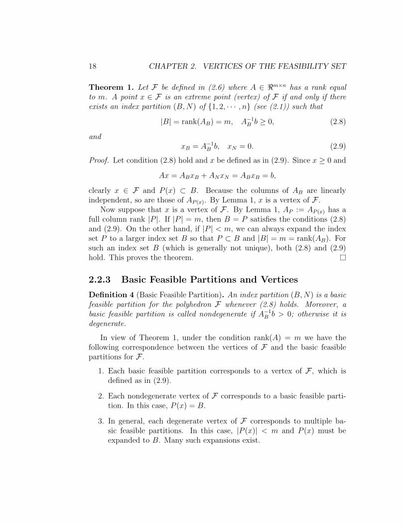
Theorem 1. Let F be defined in (2.6) where A ∈ <m×n has a rank equalto m. A point x ∈ F is an extreme point (vertex) of F if and only if thereexists an index partition (B,N) of {1, 2, · · · , n} (see (2.1)) such that

|B| = rank(AB) = m, A−1B b ≥ 0, (2.8)

andxB = A−1B b, xN = 0. (2.9)

Proof. Let condition (2.8) hold and x be defined as in (2.9). Since x ≥ 0 and

Ax = ABxB + ANxN = ABxB = b,

clearly x ∈ F and P (x) ⊂ B. Because the columns of AB are linearlyindependent, so are those of AP (x). By Lemma 1, x is a vertex of F .

Now suppose that x is a vertex of F . By Lemma 1, AP := AP (x) has afull column rank |P |. If |P | = m, then B = P satisfies the conditions (2.8)and (2.9). On the other hand, if |P | < m, we can always expand the indexset P to a larger index set B so that P ⊂ B and |B| = m = rank(AB). Forsuch an index set B (which is generally not unique), both (2.8) and (2.9)hold. This proves the theorem.

2.2.3 Basic Feasible Partitions and Vertices

Definition 4 (Basic Feasible Partition). An index partition (B,N) is a basicfeasible partition for the polyhedron F whenever (2.8) holds. Moreover, abasic feasible partition is called nondegenerate if A−1B b > 0; otherwise it isdegenerate.

In view of Theorem 1, under the condition rank(A) = m we have thefollowing correspondence between the vertices of F and the basic feasiblepartitions for F .

1. Each basic feasible partition corresponds to a vertex of F , which isdefined as in (2.9).

2. Each nondegenerate vertex of F corresponds to a basic feasible parti-tion. In this case, P (x) = B.

3. In general, each degenerate vertex of F corresponds to multiple ba-sic feasible partitions. In this case, |P (x)| < m and P (x) must beexpanded to B. Many such expansions exist.

2.3. EXERCISES 19

2.3 Exercises

1. Prove that the optimal solution set of a convex program defined in (2.5)is a convex set.

2. Consider the polytope

F = {x ∈ <4 : x1 + x2 + x3 = 1, x2 + x4 = 1, x ≥ 0}.

(a) Use Lemma 1 to determine whether or not the following points arevertices of F : (1, 0, 0, 1)T , (1

2, 12, 0, 1

2)T , and give your reasons.

(b) Use Theorem 1 to verify that the point x = (0, 1, 0, 0)T is a vertexof F . Find all possible index partitions so that the conditions of thetheorem hold.

Chapter 3

Simplex Method: First Look

3.1 Terminology

Due to historical reasons, the following terminology has been widely used inthe linear programming literature.

• Feasible solution: A set of values for the vector x that satisfy all theconstraints, including the nonnegativity.

• Basic feasible solution: A feasible solution that has m basic vari-ables taking nonnegative values and n − m nonbasic variables takingzero values. In addition, the submatrix of A corresponging the basicvariables is an m by m nonsingular matrix. The simplex method worksexclusively with basic feasible solutions.

• Degenerate basic feasible solution: A basic feasible solution thathas one or more zero basic variable. On the other hand, all basicvariables are positive in a non-degenerate basic feasible solutions.

3.2 Reduced Linear Program

3.2.1 Partitioning and Elimination

Given an index partition

B ∪N = {1, 2, · · · , n}, B ∩N = ∅

21

22 CHAPTER 3. SIMPLEX METHOD: FIRST LOOK

such that the submatrix AB of A, formed by the columns A with indices in B,is m×m and nonsingular (therefore, |B| = m and |N | = n−m). Similarly,we define AN as the submatrix of A formed by the columns A with indices inN . Accordingly, we partition x and c into [xB, xN ] and [cB, cN ], respectively.That is,

{1, 2, · · · , n} → [B | N ]A → [AB | AN ]c → [cB | cN ]x → [xB | xN ]

The actual ordering of indices inside B or N is immaterial as long as it isconsistent for all the portioned quantities.

Under such a partition where AB is nonsingular, we have the followingequivalence:

Ax = b ⇐⇒ ABxB + ANxN = b ⇐⇒ xB = A−1B (b− ANxN). (3.1)

Upon substituting the expression for xB into that for cTx, we have

cTx = cTBxB + cTNxN

= cTBA−1B b− cTBA−1B ANxN + cTNxN

= bT (A−TB cB) + (cN − ATNA−TB cB)TxN ;

or equivalently,

cTx = bTy + sTNxN , (3.2)

where we have used the short-hand notation:

y = A−TB cB and sN = cN − ATNy. (3.3)

Note that y and sN depend solely on the given data (A, b, c) and the givenpartitioning, but independent of x. They will change as the partitioningchanges.

3.2.2 Reduced Linear Program

We have used the equation Ax = b to eliminate the variables in xB fromthe original LP problem. The reduced LP problem has no more equality

3.2. REDUCED LINEAR PROGRAM 23

constraints and involves only variables in xN .

minxN

bTy + sTNxN

s.t. A−1B b− A−1B ANxN ≥ 0 (3.4)

xN ≥ 0.

The first inequality is nothing but the nonnegativity for xB. This reduced LPis completely equivalent to the original LP. However, we can deduce usefulinformation from this reduced LP that is not apparent in the original LP.

3.2.3 What Happens at A Basic Feasible Solution?

If the partitioning is associated with a basic feasible solution, then B corre-sponds to a “basis” and N to a “nonbasis” such that the “basic variables”xB = A−1B b ≥ 0 and the “nonbasic variables” xN = 0. In this case, we observethe following.

• Any feasible change that can be made to xN is to increase one or moreof its elements from zero to some positive value.

• If sN ≥ 0, then it is not possible to decrease the objective functionvalue by increasing one or more element of xN . Hence we can concludethat the current basic feasible solution is optimal.

• On the other hand, if any element of sN is negative, we can try toincrease the corresponding variable in xN , say xj in terms of the originalindexing, as much as possible so long as we maintain the inequalityconstraints in the reduced LP.

• When xj is increased from zero to t while all other elements of xNremain at zero, then ANxN becomes tAj where Aj is the j-th columnof A.

• In the above case, the first inequality in the reduced LP changes to

xB − tA−1B Aj ≥ 0.

• The problem is unbounded if the above inequality poses no restrictionon how large t can be, meaning that one can arbitrarily improve theobjective.


3.3 One Iteration of the Simplex Method

Given date A ∈ <m×n, c ∈ <n and a basic feasible solution x ∈ <n along withits corresponding index partition (B,N) with xN = 0 and xB = A−1B b ≥ 0.The indices in B and N are, respectively, in arbitrary but fixed orders.

Step 1 (Dual estimates)Solve ATBy = cB for y and compute sN = cN − ATNy.

Step 2 (Check optimality)If all sN ≥ 0, stop “Optimum Reached”.

Step 3 (Select entering variable)Choose an index q such that (sN)q < 0, and let j be the corresponding(the q-th) index in N . Here q is a local index for sN ∈ <n−m and j is aglobal index for x ∈ <n. The variable xj, currently non-basic, will beentering the basis.

Step 4 (Compute step)Solve ABd = Aj for d ∈ <m where Aj is the j-th column of A. (Thisvector d is used to update xB = A−1B b to account for the change that isto take place due to the increase in xj.)

Step 5 (Check Unboundedness)If all d ≤ 0, stop “Unbounded”.

Step 6 (Select leaving variable)Compute the largest step length t so that xB − td ≥ 0; namely,

t∗ = mindk>0

{(xB)kdk

}≡ (xB)p

dp, (3.5)

where the minimum occurs at (xB)p = xi for some index i ∈ B. Herep is a local index for xB ∈ <m and i is a global index for x ∈ <n. Thevariable xi, currently basic, will be leaving the basis.

Step 7 (Update variables)Let xj = t∗ and xB ⇐ xB − t∗d. Note that after the update the p-thbasic variable (xB)p ≡ xi is zero (and it leaves the basis and becomesnon-basic).

3.4. DO WE REACH A NEW VERTEX? 25

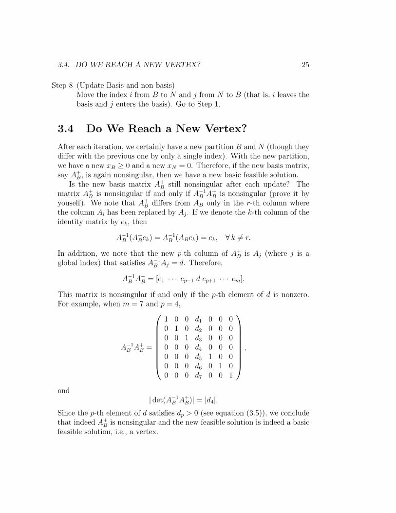
Step 8 (Update Basis and non-basis)Move the index i from B to N and j from N to B (that is, i leaves thebasis and j enters the basis). Go to Step 1.

3.4 Do We Reach a New Vertex?

After each iteration, we certainly have a new partition B and N (though theydiffer with the previous one by only a single index). With the new partition,we have a new xB ≥ 0 and a new xN = 0. Therefore, if the new basis matrix,say A+

B, is again nonsingular, then we have a new basic feasible solution.Is the new basis matrix A+

B still nonsingular after each update? Thematrix A+

B is nonsingular if and only if A−1B A+B is nonsingular (prove it by

youself). We note that A+B differs from AB only in the r-th column where

the column Ai has been replaced by Aj. If we denote the k-th column of theidentity matrix by ek, then

A−1B (A+Bek) = A−1B (ABek) = ek, ∀ k 6= r.

In addition, we note that the new p-th column of A+B is Aj (where j is a

global index) that satisfies A−1B Aj = d. Therefore,

A−1B A+B = [e1 · · · ep−1 d ep+1 · · · em].

This matrix is nonsingular if and only if the p-th element of d is nonzero.For example, when m = 7 and p = 4,

A−1B A+B =

1 0 0 d1 0 0 00 1 0 d2 0 0 00 0 1 d3 0 0 00 0 0 d4 0 0 00 0 0 d5 1 0 00 0 0 d6 0 1 00 0 0 d7 0 0 1

,

and| det(A−1B A+

B)| = |d4|.Since the p-th element of d satisfies dp > 0 (see equation (3.5)), we concludethat indeed A+

B is nonsingular and the new feasible solution is indeed a basicfeasible solution, i.e., a vertex.


3.5 Exercises

1. Let A and B are two square matrices of the same size and A is nonsin-gular. Prove that B is nonsingular if and only if A−1B is nonsingular.

Chapter 4

Simplex Method: More Details

4.1 How to Start Simplex? – Two Phases

Our simplex algorithm is constructed for solving the following standard formof linear programs:

min cTxs.t. Ax = b

x ≥ 0

where A is m × n. To start the algorithm, we need an initial basic feasiblesolution (or a vexter for the feasibility set). In general, such an initial basicfeasible solution is not readily available. Some work is required.

To be absolutely clear, what we need is essentially a partition (B,N) ofthe index set {1, 2, · · · , n}, with m indices in B, such that the basis matrixAB is nonsingular and A−1B b ≥ 0. Then we let the m basic variables to bexB = A−1B b and the rest of (non-basic) variables to be zeros. This gives us abasic feasible solution needed.

Let us see how we can start the simplex algorithm to solve the followingLP:

min cTxs.t. Ax ≤ b

x ≥ 0,(4.1)

where again A is m× n. We already know that the main constraint Ax ≤ bis equivalent to Ax + Is = b for s ≥ 0. By adding thd slack variable s, weconvert the LP into the standard form with m equations and n+m variables.The coefficient matrix bacomes A = [A I] which is m× (n+m).

27

28 CHAPTER 4. SIMPLEX METHOD: MORE DETAILS

Whenever b ≥ 0, the LP is clearly feasible since x = 0 satisfies theconstraints. It is also easy to construct an initial basic feasible solutiuon.We can simply set x = 0 as the non-basic variables and s = b ≥ 0 as them basic variables. This way, we satisfy the equation Ax + Is = b and infact obtain a basic feasible solution. This is true becarse the correspondingbasis matrix is the identity matrix and A−1B b = I ∗ b = b ≥ 0. If we orderour n + m variables in the order (x; s), then we have B = {1, 2, · · · , n} andN = {n+ 1, n+ 2, · · · , n+m}. From this partition, we can start the simplexmethod.

4.1.1 Phase-I: An Auxiliary Problem

When b is not nonnegative, however, things are more complicated. First ofall, we cannot easily tell whether the LP is feasible or not. Even it is feasible,an initial basic feasible solution is not obvious. To handle this case, we needto do a so-called phase-I procedure.

The purpose of phase-I is tow-folds. First, we would like to determinewhether the original LP is feasible or not. Second, we would like to constructan initial basic feasible solution wheneven the original LP is feasible. Towardsthis end, we consider a so-called auxiliary linear program.

Since x = 0 and s = b do not give a feasible solution when b has one ormore negative component, we consider adding another new scalar variable t,called the auxiliary variable, that is chosen to make si = bi + t ≥ 0 for eachcomponent si of s. However, since this auxiliary variable is inconsistent withthe original problem, we wish to eventually make it vanish if possible. Theauxiliary problem is the following.

min ts.t. Ax+ s− te = b

x, s, t ≥ 0.(4.2)

where t is the auxiliary scalar variable and e = (1, 1, · · · , 1)T ∈ <m is thevector of all ones. This linear program is always feasible and cannot beunbounded (prove it by yourself).

We will make the auxiliary variable t one of the basix variables and con-struct a basic feasible solution in the following manner. Recall that our ofthe n + m + 1 variables in (x; s; t), we need m basic variables and n + 1non-basic ones that are zeros.

4.1. HOW TO START SIMPLEX? – TWO PHASES 29

We still set x = 0 as our n non-basic variables, so we need one morenon-basic variable. We set

t = − min1≤i≤m

bi := −bk > 0,

namely, t takes the absolute value of the most negative element of b whichis assumed to be sk for some index k. Since t is positive, it must be a basicvariable. Now the equation Ax+ s− te = b dictates that

s = b+ te = b− bke ≥ 0,

where clearly sk = 0 (there might be other zero elements in s as well). Wemake sk to be the last non-basic variable. For example, for the vector b givenbelow, t = −b3 = 2 and

s = b+ te =

3−1−2

0

+ 2

1111

=

5102

≥ 0.

With these choices, we have (i) the feasibility: Ax + s − te = b withx, s, t ≥ 0; (ii) m basic variables, in t and in the m − 1 components of sexcluding sk; (iii) n + 1 non-basic variables, in x = 0 and in sk = 0. Thebasis matrix consists of the m− 1 columns of the identity matrix excludingthe k-th column, plus the column −e. It is nonsingular. So we have found abasic feasible solution for the auxiliary problem!

Starting from this basic feasible solution, we can use simplex method tosolve the auxiliary problem. In the subsequent simplex iterations, we shouldalways let t have the priority to leave the basis whenever it qualifies as acandidate. Once t leave the basis, the optimal objective value is reached.

At the optimality, if t = 0, then the original LP is feasible; otherwise(t > 0), it must be infeasible and we stop here.

4.1.2 Phase-II: The Original Problem

In the case where the original problem is feasible, we delete the columncorresponding to the auxiliary variable t (it’s non-basic and zero anyway)from the auxiliary problem, and shrink the non-basis by one. This producesa basic feasible solution for the original problem (since t is gone), from whichwe can start the simplex method to solve the original problem.


4.2 Main Implemetational Issues

We observe that in the revised simplex algorithm, the main computationaltask appears to be solving two linear systems of equations: one in Step 1 andanother in Step 4. The two systems involve the same matrix AB, though itappears in Step 4 as the transpose.

(TBC)

4.3 Degeneracy, Cycling and Stalling

So far everything sounds so rosy. But there is one place where things cango wrong. That is, what if xB has a zero component which happens tocorrespond to a positive component of d. In this case, t∗ = 0 in (3.5), andno real change whatsoever, except for the partitioning, has been made to thevariables. The objective value also remains the same. When this happens toa simplex iteration, such an iteration is called a degenerate simplex iteration.This situation is also called stalling. What are the consequences of degenerateiterations?

First of all, degenerate iterations that make no progress are not produc-tive. At the least, they slow down the convergence if convergence eventuallyoccur. Indeed, in the worst case, it can prevent convergence from occuring.This phenomenon is called cycling where the simplex method keeps changingbasis but going on circle. Namely, after a while it comes back to a basis thathas been visited before, while staying at the same vertex.

There exist some deliberate pivoting procedures (for choosing enteringand leaving variables) that can avoid cycling. Fortunately, as dangerous asit is in theory, cycling almost never happens in practice and therefore is notof a real concern. On the other hand, generacy does cause real problemsfor simplex methods because it occurs so frequently, even more often thannondegeneracy, in practice (well, people prefer redundancy than inadequacy),and it can significantly degrade the performance of simplex methods.

4.4 Exercises

1. Prove that the auxiliary LP is feasible and cannot be unbounded.

2. Prove that an m × m matrix consists of the m − 1 columns of the

4.4. EXERCISES 31

identity matrix plus the column −e, where e ∈ <m is the vector of allones, is nonsingular.

3. Let us arrange the variables in the order x; s; t with n variables in x, mvariables in s and one variable in t. Write down the index sets B andN for the initial basic feasible solution constructed for the auxiliaryproblem.

4. Prove that if the optimal value of the auxiliary LP is positive, then theoriginal LP is infeasible. Otherwise, it is feasible.

5. For the general standard-form LP: min{cTx : Ax = b, x ≥ 0}, con-struct an auxiliary LP and an initial basic feasible solution for it. (Hint:Put s in the objective.)

Chapter 5

Duality and OptimalityConditions

5.1 Dual Linear Program

Consider our standard form linear program (1.4) again, i.e.,

min cTxs.t. Ax = b

x ≥ 0

where A is m × n with m < n and full-rank, the the sizes of all the otherquantities follow accordingly. The reduced LP corresponding to (1.4) is

minxN

bTy + sTNxN

s.t. A−1B b− A−1B ANxN ≥ 0

xN ≥ 0.

From this reduced LP, we can make the following observation.

Proposition 3. If there is a partition (B,N) of the index set {1, 2, · · · , n}such that (i) A−1B b ≥ 0; (ii) sN = cN − ATNy∗ ≥ 0 for y∗ = A−TB cB, then x∗

solves the LP where x∗B = A−1B b and x∗N = 0. Moreover, the optimal objectivevalue satisfies cTx∗ = bTy∗.

Therefore, conditions (i)-(ii) are sufficient for optimality. In the nonde-generate case where (i) becomes A−1B b > 0, condition (ii) is clearly necessaryfor optimality.

33

34 CHAPTER 5. DUALITY AND OPTIMALITY CONDITIONS

Condition (ii) can be rewritten as cB − ATBy∗ = 0 and cN − ATNy∗ ≥ 0,which implies that y∗ satisfies

c− ATy ≥ 0 or ATy ≤ c. (5.1)

It turns out that for any y satisfying (5.1) and any feasible x (satisfyingAx = b and x ≥ 0), the following inequality holds

bTy = (Ax)Ty = xT (ATy) ≤ xT c = cTx,

where we have used the facts Ax = b, x ≥ 0 and ATy ≤ c. Consequently,

maxy{bTy : ATy ≤ c} ≤ min

x{cTx : Ax = b, x ≥ 0}, (5.2)

as long as both extreme values exist.The right-hand side is nothing but our linear program (1.4). Appearing

on the left-hand side is another linear program, which can also be written as

max bTys.t. ATy + s = c

s ≥ 0(5.3)

where a slack variable s is added.Obviously, this pair of linear programs share the same set of data (A, b, c)

and are closely related. We call (1.4) the primal LP and (5.3) the dual LP.Whenever this primal-dual pair of LPs are both feasible, they satisfy theproperty in (5.2) which is called weak duality. We now formally state theweak duality as follows.

Proposition 4 (Weak Duality). If x is primal feasible and y is dual feasible,then bTy ≤ cTx. As a result, (5.2) holds true.

The objective values of the primal and the dual serve as bounds for eachother. Once they coincide, then they must have reached their optimal valuessimultaneously. In fact, optimality can occur only if the primal and the dualobjective values coincide. This property is called strong duality.

Proposition 5 (Strong Duality). A primal feasible x∗ is optimal for theprimal if and only if there is a dual feasible y∗ such that cTx∗ = bTy∗. In thiscase, y∗ is optimal for the dual.

5.2. OPTIMALITY CONDITIONS 35

5.2 Optimality Conditions

Strong duality states that the optimality of the primal is inseparable fromthat of the dual. The pair is one entity as far as optimality is concerned.Now we can state the optimality conditions for the pair as follows.

Proposition 6 (Optimality Conditions). The points x∗ and y∗ are optimalfor the primal and the dual, respectively, if and only if they together satisfy(1) the primal feasibility: Ax = b and x ≥ 0; (2) the dual feasibility ATy ≤ c;and (3) the closure of the duality gap: cTx− bTy = 0.

5.3 How to find a dual?

We have seen that as far as optimality conditions are concerned, a linearprogram is inseparable with its dual and vice versa. Hence, being able tofind a dual for any given LP is crucial. There exist mathematical techniquesfor finding duals that are applicable not only to linear programming but alsoto more general problem classes. It is also possible to always convert an LPto one of the standard forms, get the corresponding dual and then simplify.Nonetheless, for linear programming it is much easier to just follow a verifiedrecipe.

For convenience, we will classify constraints into two classes: (1) signrestrictions and (2) main constraints. A sign restriction on a variable xi iseither xi ≥ 0 or xi ≤ 0. A variable without any sign restriction is calleda free variable. Any constraint that is not a sign restriction is treated as amain constraint which can be an equality or an inequality. The coefficientsfor all main constraints form an m by n coefficient matrix A ∈ <m×n, i.e.,there are n variables and m main constraints.

We consider the following linear program of a general form:

min /max cTx

s.t. aTi x

≥ bi= bi≤ bi

i = 1, 2, · · · ,m,

xj

≥ 0free≤ 0

j = 1, 2, · · · , n,

(5.4)


where aTi is the i-th row of A. In this LP, the objective can be either min-imization or maximization, and each constraint and each variable can take,respectively, one of the three given forms. The recipe for finding a dual forthus LP is given in the following chart, where if an LP is a minimizationproblem, we go from the left column to the right column to find its dual;otherwise, we go from right to left.

minimization ⇔ maximizationrhs/obj vectors ⇔ obj/rhs vectors

[coefficients] ⇔ [coefficients]T

#variables ⇔ #constraints#constraints ⇔ #variablesvariable ≥ 0 ⇔ constraint ≤variable free ⇔ constraint =variable ≤ 0 ⇔ constraint ≥constraint ≥ ⇔ variable ≥ 0constraint = ⇔ variable freeconstraint ≤ ⇔ variable ≤ 0

Figure 5.1: Chart for Finding a Dual

The chart says that to find a dual for a given primal, we flip the opti-mization goals, switch the objective and right-hand side vectors, and take atranspose of the coefficient matrix for the main constraints. This way, thenumbers of (main) constraints and variables in the dual are always equal to,respectively, the numbers of variables and constraints in the primal, and viceversa. In addition, the types of the constraints and variables follow the rulesstipulated in the chart. The chart also reveals one-to-one relationships be-tween the variables in the primal and the constraints in the dual and viceversa.

Example 1. Find the dual of ...

Now let us use the chart to find the dual of the general LP 5.4. Wepartition the index set {1, 2, · · · ,m} into three subsets:

1. G corresponding to constraints of the type aTi x ≥ bi;

5.3. HOW TO FIND A DUAL? 37

2. E corresponding to constraints of the type aTi x = bi;

3. L corresponding to constraints of the type aTi x ≤ bi.

Similarly, we partition the index set {1, 2, · · · , n} into three subsets:

1. P corresponding to variables of the type xi ≥ 0;

2. F corresponding to free variables;

3. M corresponding to variables of the type xi ≤ 0.

Now we partition the rows of A according to the partition (G,E,L), and thecolumns of A according to the partition (P, F,M); namely,

A =

AG

AE

AL

=[AP AF AM

]. (5.5)

With these partitions, we can write (5.4) into the following form:

min cTxs.t. AGx ≥ bG

AEx = bEALx ≤ bLxP ≥ 0xF freexM ≤ 0.

(5.6)

The dual readily follows from the chart in Figure 5.1.

max bTys.t. ATPy ≤ cP

ATFy = cFATMy ≥ cMyG ≥ 0yE freeyL ≤ 0

(5.7)

The complementarity conditions for this pair of primal-dual LPs are(AGx− bG) ◦ yG(ALx− bL) ◦ yLxP ◦ (cP − ATPy)xM ◦ (cM − ATMy)

= 0. (5.8)


It is possible that some of these subsets are empty, in which case thecorresponding constraints/variables are in non-existence. For example, ifM = ∅, then the variable xM and its dual constraint ATMy ≥ cM do not exist.

5.4 Exercises

1. Use the weak duality to show that if the primal is unbounded then thedual must be infeasible and vice versa.

2. Prove that for feasible x and y, the duality gap satisfies

cTx− bTy = sTx

where s = c− ATy ≥ 0 is the dual slack.

3. At each iteration of the primal simplex method, out of the three opti-mality conditions, which is satisfied and which is not? Explain.

Chapter 6

Primal-Dual Interior-PointMethods

6.1 Introduction

Consider the following primal linear program:

min cTxs.t. Ax = b

x ≥ 0(6.1)

where c, x ∈ <n, b ∈ <m and A ∈ <m×n(m < n).Its dual linear program is:

max bTys.t. ATy + z = c

z ≥ 0(6.2)

where z ∈ <n is the vector of dual slack variables.A primal-dual method is one that treats the primal and the dual equally

and tries to solve both at the same time.For feasible x and (y, z), the duality gap is

cTx− bTy= xT c− xTATy (Ax = b)= xT (c− ATy)= xT z (c− ATy = z)≥ 0 (x, z ≥ 0).

39

40 CHAPTER 6. PRIMAL-DUAL INTERIOR-POINT METHODS

Duality gap is closed at optimality:

cTx∗ − bTy∗ = (x∗)T z∗ = 0.

The complementarity conditions are:

x∗i z∗i = 0, i = 1, 2, . . . , n. (6.3)

6.2 A Primal-Dual Method

Consider F : R2n+m → R2n+m,

F (x, y, z) =

ATy + z − cAx− bx1z1

...xnzn

= 0. (6.4)

This is a linear-quadratic square system.The optimality conditions for the linear program is

F (x, y, z) = 0, (x, z) ≥ 0. (6.5)

It is also called the KKT (Karush-Kohn-Tucker) system for the LP.The Jacobian matrix of F (x, y, z) is

F ′(x, y, z) =

0 AT IA 0 0Z 0 X

, (6.6)

where X = diag(x) and Z = diag(z). F ′(x, y, z) is nonsingular for (x, z) > 0if A has full rank.

Even though (6.5) is just mildly nonlinear, one should not expect thatthe pure Newton’s method would solve the system because of the presenceof nonnegativity constraints on x and z.

A main idea for interior-point methods is that one starts from an initialpoint with x > 0 and z > 0 and forces all subsequent iterates for x and z toremain positive, i.e., to stay in the interior of the nonnegative orthant. One

6.2. A PRIMAL-DUAL METHOD 41

can always enforce this interiority requirement by choosing appropriate stepparameter in a dampled Newton setting.

It is important to note the necessity of keeping the nonnegative variables xand z strictly positive at every iteration instead of just nonnegative. Considera scalar complementarity condition xz = 0, x, z ∈ <. The Newton equation(i.e., the linearized equation) for xz = 0 at a given point (x, z) is xdz+ zdx =−xz. If one variable, say z, is zero, and the other is nonzero, then the Newtonequation becomes xdz = 0, leading to a zero update dz = 0. Consequently,z will remain zero all the time once it becomes zero. This is fatal becausean algorithm will never be able to recover once it mistakenly sets a variableto zero. Therefore, it is critical to keep the nonnegative variables strictlypositive at every iteration, not just nonnegative.

Even keeping nonnegative variables strictly positive, one would still ex-pect difficulty in recovering from a situation where a variable is adverselyset to too small a value. To decrease the chances of such mistakes at earlystages, it would be desirable that all the complementarity pairs converge tozero at the same pace, namely xki z

ki = µk→0 as k→∞ for every index i.

Towards this goal (and for other theoretic considerations as well), one canperturb each complementarity condition xizi = 0 into xizi − µ = 0 and let µgo to zero in a controlled fashion. This idea, incorporated into the dampedNewton method, leads to the following primal-dual interior-point algorithm.Recall that it is called primal-dual because it treats the primal and dualvariables equally.

Like in any iterative method, we need some initial point to start. Inparticular, we need positive x and z in our initial point. A simple, and notso bad, initial point consists of x = z = n ∗ e, where e is the vector of allones, and y = 0.

Algorithm 1 (A Prima-Dual Interior Point Algorithm).

Choose initial point (x > 0, y, z > 0).

WHILE “stopping criteria” not satisfied, DO

Step 1 Choose σ ∈ (0, 1) and set µ = σxT z/n.

Step 2 Solve the linear system for (dx, dy, dz)

F ′(x, y, z)

dxdydz

= −F (x, y, z) +

00µe

.


Step 3 Compute the primal and dual step-length parameters:

αp = −1/min([X−1dx;−1]), αd = −1/min([Z−1dz;−1]).

Step 4 Choose τ ∈ (0, 1) and update xyz

⇐=

xyz

+ τ

αp dxαd dyαd dz

.END

We now make the following observations on the algorithm. There aretwo basic parameters in the algorithm: σ in Step 2 and τ in Step 4. Theirsensible choices are of vital importance to both the theoretical analysis andthe practical performance of the algorithm. For starters, however, σ = .2and τ = .99, say, will work fine most of the time.

In Step 3, each minimum is taken as the smallest element of the corre-sponding n+1-dimensional vector. The scalars αp and αd are the largest steplengths in [0, 1] such that x+αp dx ≥ 0 and z+αd dz ≥ 0, respectively. (Theformulas are nothing but compact expressions of the ratio tests performed insimplex methods.)

In Step 4, tha parameter τ is chosen to step back a little from the bound-ary of the positive orthant where the next iterate might land had a full stepαp or αd been taken. By choosing τ ∈ (0, 1), the posititivity for the variablesx and z will always hold. If the algorithm converges, it does converge most ofthe time even for rather naive choices of parameters, then some componentsof x and z will go to zero in order to satisfy the complementary slackness con-ditions Xz = 0. Namely, the iterates will eventually approach the boundaryof the positive orthant.

The step computed in Step 2 is the Newton step for the so-called per-turbed KKT equation

Fµ(x, y, z) ≡ F (x, y, z)− µk

00e

= 0,

namely, the complementarity equation Xz = 0 is perturbed into Xz = µe.This perturbation tends to keep all components of Xz equal and, hopefully,forces them to converge to zero at more or less the similar pace.

6.3. SOLVING THE LINEAR SYSTEM 43

Overall, we may view the algorithm as a perturbed and damped New-ton method.

Finally, we state a reasonable stopping criterion

‖Ax− b‖1 + ‖b‖

+‖ATy + z − c‖

1 + ‖c‖+|cTx− bTy|1 + |bTy|

≤ tolerance,

where we use the sum of the relative errors in the three blocks of equationsto measure the total error.

6.3 Solving the Linear System

The main computation in Algorithm 1 at each iteration is to solve to thelinear system in Step 2 involving the coefficient matrix F ′(x, y, z) which is2n+m by 2n+m but very sparse (see (6.6)). This system can be written as

ATdy + dz = rd, (6.7)

Adx = rp, (6.8)

Zdx+Xdz = rc, (6.9)

where X = diag(x) and Z = diag(z) are diagonal matrices and

rd = c− ATy − z, rp = b− Ax, rc = µe−Xz.

Multiplying (6.7) by X and subtract (6.9) from it, we obtain

XATdy − Zdx = Xrd − rc.

Multiplying the above equation by AZ−1 and invoking (6.8), we arrive ata square system for dy in (6.10). After dy is computed, we can then easilycompute dz and dx by back substitution using (6.7) and (6.9). Hence aprocedure for solving the linear system is as follows:

(AZ−1XAT ) dy = AZ−1(Xrd − rc) + rp, (6.10)

dz = rd − ATdy, (6.11)

dx = Z−1(rc −Xdz), (6.12)

Now the major computation becomes solving (6.10) which is an m by msystem with a positive definite coefficient matrix provided that A has fullrank. (For large-scale problems, (6.10) is usually solved by sparse Choleskyfactorization.)


6.4 Convergence Considerations

To guarantee in theory that the primal-dual interior-point algorithm, Algo-rithm 1, always converges to a solution, one needs to use rather sophisti-cated schemes to choose the step parameter τ . On the other hand, even withsimple-minded choices such as τ = 0.9, the algorithm does converge mostof the time for problems that are not particularly difficult. Here we providesome indications on why the algorithm usually works even for choices suchas τ = 0.9.

At each iteration, given the current iterate (x, y, z) the update direction(dx, dy, dz) satisfies the equation

Adx = −(Ax− b), ATdy + dz = −(ATy + z − c),

and the next iterate (x+, y+, z+) is calculated as x+

y+

z+

=

xyz

+ α

dxdydz

, (6.13)

for some α ∈ (0, 1]. Here for simplicity we are using the same step parameterfor both the primal and the dual variables. By direct substitution we have

Ax+− b = (1− α)(Ax− b), ATy+ + z+− c = (1− α)(ATy+ z− c). (6.14)

Since 1− α ∈ [0, 1), we have the following relationships

‖Ax+ − b‖ = (1− α)‖Ax− b‖ < ‖Ax− b‖,‖ATy+ + z+ − c‖ = (1− α)‖ATy + z − c‖ < ‖ATy + z − c‖.

That is, we can improve the primal and dual feasibility at each iteration.However, such improvements do not imply that the iterates necessarily con-verge to a feasible (primal and dual) point (the improvements could shrinkto zero as α → 0). Moreover, it is not clear that we can also improve thecomplementary slackness at each iteration.

To simplify the matter, let us assume that the initial point (x0, y0, z0) isstrictly feasible, i.e., it satisfies

Ax0 = b, ATy0 + z0 = c, x0, z0 > 0.

6.4. CONVERGENCE CONSIDERATIONS 45

It follows from the recursive relationships (6.14) that the feasibility of (x0, y0, z0)implies the feasibility of (xk, yk, zk) for k = 1, 2, · · · . In this case,

F (xk, yk, zk) =

00

Xkzk

and

‖F (xk, yk, zk)‖1 =n∑i=1

xki zki = (xk)T (zk).

Hence, it suffices to consider driving the duality gap xT z to zero.Now consider the duality gap at (x+, y+, z+), where (x+, y+, z+) is ob-

tained from the update formula (6.13). Hence,

(x+)T (z+) = (x+ αdx)T (z + αdz)

= xT z + α(xTdz + zTdx) + α2(dx)T (dz)

= xT z + α(xTdz + zTdx) [(dx)T (dz) = 0]

= xT z + αeT (µe−Xz) [Xdz + Zdx = µe−Xz]= xT z + α(σ − 1)xT z [µ = σxT z/n]

= [1− α(1− σ)]xT z.

We leave the fact (dx)T (dz) = 0 as an exercise. Since by our choice α ∈ (0, 1]and σ ∈ (0, 1), we have the recursive relationship

(x+)T (z+) = [1− α(1− σ)]xT z < xT z,

that is, the algorithm always decreases the duality after each iteration. Moreprecisely,

(xk)T (zk) = [1− αk−1(1− σ)](xk−1)T (zk−1) = · · ·

=

(k−1∏j=0

[1− αj(1− σ)]

)(x0)T (z0).

If the step parameters αj are bounded below by a nonzero shortest step α,i.e., αj ≥ α, then for all j

1− αj(1− σ) ≤ 1− α(1− σ) < 1.


Consequently,

0 ≤ (xk)T (zk) ≤ [1− α(1− σ)]k(x0)T (z0)→ 0 as k →∞,

which implies the convergence of the duality gap to zero, and hence theconvergence of the algorithm. Indeed, we observe that the step parameterα rarely shrinks to zero. That is one of the reasons the algorithm usuallyworks even for naive choices of step parameter.

Appendix A

Introduction to Newton’sMethod

One of the fundamental computational problems in science and engineeringis to solve nonlinear systems of equations of multiple variables. A generalnonlinear, square system of equations can be expressed as follows:

F (x) = 0, (A.1)

where x ∈ <n and F : <n → <n; namely, there are n variables and nequations. We will assume that not all of the n equations are linear; otherwise(A.1) becomes a linear system which is much easier to solve. In a moredetailed notation, we have

x =

x1x2...xn

, F (x) =

F1(x)F2(x)

...Fn(x)

≡F1(x1, x2, · · · , xn)F2(x1, x2, · · · , xn)

...Fn(x1, x2, · · · , xn)

,where we use the subscripts to denote components of vectors. For example,a simple nonlinear system with n = 2 is

F (x) =

[e2x1 − ex2x21 + x22 − 5

]= 0. (A.2)

At a given point xc ∈ <n (note that we use a superscript to denotea particular vector), considered as the current approximate solution to the

47

48 APPENDIX A. INTRODUCTION TO NEWTON’S METHOD

equation F (x) = 0, we approximate F (x) by its first-order Taylor expansion:

F (x) ≈ Lc(x) ≡ F (xc) + F ′(xc)(x− xc),

where F ′(x) is an n× n matrix called the Jacobian matrix of F (x), which isthe first derivative of F (x). The entries of the Jacobian matrix F ′(x) consistof all the first-order partial derivatives of the component functions Fi(x)’s,arranged in an ordered fashion, i.e.,

[F ′(x)]ij =∂Fi(x)

∂xj, 1 ≤ i, j ≤ n.

In other words, the i-th row of F ′(x) is the gradient of Fi(x). For example,when n = 2, F ′(x) is a 2× 2 matrix,

F ′(x) =

∂F1(x)∂x1

∂F1(x)∂x2

∂F2(x)∂x1

∂F2(x)∂x2

.In particular, the Jacobian of the function F (x) in (A.2) is

F ′(x) =

[2e2x1 −ex22x1 2x2

]. (A.3)

We note that since xc is a fixed point, F (xc) is a fixed n-vector and F ′(xc)a fixed n × n matrix. Hence Lc(x) is a linear function of x and called thelinearization of F (x) at the point xc.

Solving the square linear system of equations Lc(x) = 0, we obtain apoint x+ as a new approximate solution to the equation F (x) = 0. It is easyto verify that the solution to Lc(x) = 0 is

x+ = xc − [F ′(xc)]−1F (xc),

provided that F ′(xc) is nonsingular. We leave the verification to the reader.In the case of n = 1, both F (x) and its derivative F ′(x) are scalar func-

tions. The linearization of F (x) at xc,

y = Lc(x) ≡ F (xc) + F ′(xc)(x− xc), (A.4)

is the tangent line of the curve y = F (x) at the point x = xc. The newapproximate solution,

x+ = xc − F (xc)

F ′(xc), (A.5)

49

Figure A.1: Newton’s method: one-dimensional case

is the intersection of the tangent line y = Lc(x) with the x-axis y = 0, seeFigure A.

In the general case of n variables and n equations, Newton’s methodcomputes the iteration sequence {xk} ⊂ <n by the recursive formula:

xk+1 = xk − [F ′(xk)]−1F (xk),

starting from a given initial point x0. If x0 is sufficiently close to a solutionx∗ satisfying F (x∗) = 0, then under proper conditions, we can expect thatthe sequence converges to the solution x∗; namely,

limk→∞

xk = x∗.

The main idea behind Newton’s method can be described as follows. Insteadof trying to directly solve the hard problem, the nonlinear system, one solvesa sequence of easy problems, the linear systems, to obtain a sequence ofapproximate solutions that will hopefully get closer and closer to the truesolution.

Introducing a step parameter αk ∈ (0, 1] at each iteration, we obtain theso-called damped Newton’s method:

xk+1 = xk − αk[F ′(xk)]−1F (xk).

It is known that properly chosen step parameters can help enhance the con-vergence of Newton’s method, which is corresponding to the case whereαk = 1 for all k.


A.1 An Example

Let us consider solving the simple nonlinear system defined in (A.2), namely,

F (x) =

[e2x1 − ex2x21 + x22 − 5

]= 0.

It has two equations and two variables. Incidently, it also has two solutions:x = [1; 2] and x = [−1;−2]. The Jacobian matrix of this function is given in(A.3).

The following Matlab functions implement Newton’s method for solvingthe nonlinear system (A.2).

% main program

function x = newton(x0);

% input x0 -- the starting point

% output x -- hopefully a solution

% make x0 a column vector if not already

if size(x0,1) < size(x0,2) x0 = x0’; end;

x = x0;

iter = 1; % iteration counter

tol = 1.e-8; % error tolerance

maxiter = 50; % maximum iteration

while iter <= maxiter % begin loop

F = func(x); % evaluate F(x)

resnrm = norm(F); % residual norm

% print out information at each iteration

fprintf(’iter %2i residual-norm = %8.2e’,iter,resnrm);

fprintf(’ x = [%7.4f %7.4f]\n’,x);

% stopping criterion

if resnrm < tol disp(’Converged!’); break; end

J = jacobian(x); % evaluate Jacobian

x = x - J\F; % update iterate

iter = iter + 1; % increment counter

A.2. EXERCISES 51

end % end loop

% function evaluation

function F = func(x)

F = [exp(2*x(1))-exp(x(2));

x(1)^2+x(2)^2-5];

% Jacobian evaluation

function J = jacobian(x)

J = [2*exp(2*x(1)) -exp(x(2));

2*x(1) 2*x(2)];

These Matlab functions are saved into a file called newton1.m and can beinvoked with an initial point x0 = [1.5 1.5] by typing: newton1([1.5 1.5])

in Matlab. The output from Matlab is as follows.

newton1([1.5 1.5]);

iter 1 residual-norm = 1.56e+001 x = [ 1.5000 1.5000]

iter 2 residual-norm = 2.96e+000 x = [ 1.1673 1.9994]

iter 3 residual-norm = 3.93e-001 x = [ 1.0228 1.9937]




Converged!

For this initial point, which is fairly close to the solution x∗ = [1 2],Newton’s method takes six iterations to achieve the required accuracy.

A.2 Exercises

1. Justify the following claims:(a) y = `c(x) in (A.4) is the tangent line of the curve y = F (x) at thepoint x = xc.(b) x+ in (A.5) is the intersection of the tangent line with the x-axis.

2. Run newton1.m with initial guesses

x0 = [1 2] + a ∗ [1 1], a = 2, 4, 6, 8, 10


and answer the following questions.(a) Does Newton’s method always converge?(b) When Newton’s method converges, does it always converge to thesolution closest to the initial point?(c) When Newton’s method converges, describe how the residual norm‖F (xk)‖ decreases at each iteration towards the end.

3. Write an M-file newton2.m, by modifying the functions in newton1.m,to solve the following nonlinear system:

F (x) =

x1 + x2 − 1x3 − x4 − 1x3 − x5 − 2

x1x4x2x5

= 0

with the starting points x = [1 2 3 2 1] and x = [10 .1 10 .1 10].(Observe that for the second starting point, the obtained solution isNOT nonnegative.)

Lecture Notes for CAAM 378 A Quick Introduction to …yzhang/caam378/Notes/lec_notes.pdf · A Quick...

Documents

Transcript of Lecture Notes for CAAM 378 A Quick Introduction to …yzhang/caam378/Notes/lec_notes.pdf · A Quick...