TIGHT GAS SANDSTONERESERVOIRS, PART 1: OVERVIEWAND LITHOFACIES

14Y. Zee Ma1, W.R. Moore1, E. Gomez1, W.J. Clark1, Y. Zhang2

Schlumberger, Denver, CO, USA1; University of Wyoming, Laramie, WY, USA2

14.1 INTRODUCTION AND OVERVIEWAlthough shale gas plays have been in the spotlight recently, natural gas in tight sandstones is actuallyalso an important hydrocarbon resource. In many cases, tight gas sandstone resources can be devel-oped more easily than shale gas reservoirs as the rocks generally have higher quartz content, and aremore brittle and easier to complete for production.

This chapter first gives an overview of evaluating tight gas sandstone reservoirs, including theirdepositional environments, and other reservoir characteristics. Then, it presents an integrated meth-odology for lithofacies analysis and modeling. Because identification of lithofacies and rock typing isa key to characterizing these types of reservoirs (Rushing et al., 2008), we discuss lithofacies clas-sification using wireline logs. We present methods on how to populate the lithofacies data from wellsto a three-dimensional (3D) model while discussing the advantages and disadvantages of each methodfor modeling tight gas formations.

The next chapter is the second part of tight gas sandstone reservoirs, in which petrophysicalanalysis, formation evaluation, and 3D modeling of petrophysical properties are presented.

14.1.1 BACKGROUNDTight gas sandstone reservoirs are natural extensions of conventional sandstone reservoirs, but withlower permeability and generally lower effective porosity. Hydrocarbons have traditionally been pro-duced from sandstone and carbonate reservoirs with high porosity and permeability. Sandstone reser-voirs with permeability lower than 0.1 milliDarcy (mD) were historically not economically producible,but advances in stimulation technology have enabled production from these tight formations. There issome confusion regarding the definition of tight gas sandstone reservoirs; they are sometimes referredto as deep-basin, basin-centered gas accumulation, or pervasive sandstone reservoirs (Meckel andThomasson, 2008). The United States Gas Policy Act of 1978 classified tight gas formations as thosethat have in situ permeability less than 0.1 mD (Kazemi, 1982). Thus, sandstone gas reservoir in whichthe formation has average permeability lower than 0.1 mD is a tight gas play regardless of its depo-sitional environment. These reservoirs can occur in numerous settings, including channelized fluvialsystems (e.g., the Greater Green River basin, Law, 2002; Shanley, 2004; Ma et al., 2011), alluvial fans,

CHAPTER

Unconventional Oil and Gas Resources Handbook. http://dx.doi.org/10.1016/B978-0-12-802238-2.00014-6

Copyright © 2016 Elsevier Inc. All rights reserved.405

delta fan, slope and submarine fan channels deposits (e.g., Granite Wash, Wei and Xu, 2015), or shelfmargin (e.g., Bossier sand, Rushing et al., 2008), among others. Some tight gas sandstones containdifferent depositional facies; the Cotton Valley formation, for example, includes stacked shoreface/barrier bar deposits, tidal channel, tidal delta, inner shelf, and back-barrier deposits. Because of thevariety of depositional environments for sandstones and other variations, there is no typical tight gassandstone reservoir (Holditch, 2006a). While drilling, well design, and completion techniques forproducing a tight sandstone reservoir are often similar to producing a shale gas reservoir, explorationand resource evaluation for them generally are quite different (Kennedy et al., 2012).

Tight gas production was first developed in the San Juan Basin of the western United States;large-scale development of tight gas sandstone reservoirs has a longer history than large-scaledevelopment of shale gas reservoirs. Approximately 1 trillion cubic feet (Tcf) was produced peryear by 1970 in the United States (Naik, 2003). Meckel and Thomasson (2008) distinguished threeperiods of evolution for the evaluation and production of tight gas sandstone reservoirs: preparadigmperiod (1920–1978), paradigm period (1979–1987), and mop-up period (1988–present). The para-digm period was marked by Master’s article (1979), arguing the extensive existence of hydrocarbonresources in tight formations. Many of the basins that contain gas in tight sandstones in NorthAmerica have already been in exploration or production phase, playing an important role in theNorth American energy equation. In fact, as clastic formations are found in many parts of the world,tight gas sands make up an important resource worldwide. Rogner (1997) has estimated theworldwide tight gas resource to be approximately 7500 Tcf, but other estimates carry a much largernumber for tight gas plays (Naik, 2003). In comparison, the worldwide shale gas resource has beenestimated to be 16,100 Tcf (Rogner, 1997).

14.1.2 BASIN-CENTERED EXTENSIVE DEPOSITS OR CONVENTIONAL TRAPSTwo schools of thought exist regarding the geologic control of tight gas sandstone reservoirs:continuous basin-centered gas accumulations or BCGAs (Law, 2002; Schmoker, 2005), and gasaccumulation in low-permeability tight sandstones of a conventional trap (Shanley et al., 2004). Thedifference between these two theories can have a huge impact on the strategy for gas exploration intight sandstones and the estimate of worldwide gas resources in these formations (Aguilera andHarding, 2008).

As a matter of fact, conventional traps represent more limited, favorable structural and/orstratigraphic setups that enable natural gas accumulation after its generation and migration. Theyare thus rather geologically circumstanced. On the other hand, the BCGA theory implies acontinuous basin-wide gas accumulation, or at least widely spread within a basin. Law (2002)argued that BCGAs contained extremely large gas resources, and were one of the more economicallyviable unconventional gas resources, but there was generally a poor understanding of BCGAs despitea significant body of work on defining characteristics of gas-saturated reservoirs. These includestudies in the deep basin of Alberta, the San Juan basin of New Mexico and Colorado by Masters(1979), and the Greater Green River basin and Great Divide basin of the western United States (Lawand Spencer, 1989; Law, 1984; Spencer, 1989). According to Law (2002), the BCGA must meet thefollowing five criteria (Camp, 2008): (1) large regional extent, measuring tens of miles in diameter;(2) low permeability, less than 0.1 mD; (3) abnormal pressure (either overpressured or under-pressured); (4) gas saturated; and (5) absence of downdip water contacts. Figure 14.1 illustrates the

406 CHAPTER 14 TIGHT GAS SANDSTONE RESERVOIRS, PART 1

main characteristics of BCGS theory. One important characteristic in this theory is that the trappingmechanism is a diffused capillary-pressure seal instead of conventional structural or stratigraphiccontrols.

Shanley et al. (2004) argued that low-permeability reservoir systems such as those found in theGreater Green River basin were not examples of BCGAs, and they suggested that only trulycontinuous-type gas accumulations were to be found in hydrocarbon systems in which gas entrapmentwas dominated by adsorption. Studies on several tight gas sandstone reservoirs in the Greater GreenRiver Basin have suggested that subtle structural and stratigraphic traps better explain the primarycontrols for the hydrocarbon accumulations (Camp, 2008).

14.1.3 GENERAL PROPERTIES OF TIGHT GAS SANDSTONE RESERVOIRSAlthough the two theories, the BCGA and conventional trapping mechanism, have significant dif-ferences regarding the exploration strategies of tight gas sandstone reservoirs, none of them denies theimportance of formation evaluation in any given tight gas play.

14.1.3.1 Source rockSource rock is important for all hydrocarbon resource accumulations. For tight gas sands, the sourcerock should be in proximity to the relatively porous deposit so that the expulsion can drive the gas intothe porous formation and form the reservoir (Meckel and Thomasson, 2008). The total organic carbonof the source rock should be large enough for generation of a significant amount of hydrocarbon.

FIGURE 14.1

A schematic cross-section view illustrating BCGA model.

Modified from Schenk and Pollastro (2002).

14.1 INTRODUCTION AND OVERVIEW 407

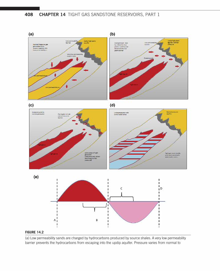
FIGURE 14.2

(a) Low permeability sands are charged by hydrocarbons produced by source shales. A very low permeability

barrier prevents the hydrocarbons from escaping into the updip aquifer. Pressure varies from normal to

408 CHAPTER 14 TIGHT GAS SANDSTONE RESERVOIRS, PART 1

Moreover, the source rock should be subjected to heat transformation within the gas-generationwindow under burial history. Therefore, it is good practice to select exploration targets proximal toorganically rich intervals (Coleman, 2008).

14.1.3.2 Abnormal PressuresThe productive intervals of a tight gas sandstone reservoir, in general, are abnormally pressured,either overpressured or underpressured (Meckel and Thomasson, 2008). The formation pressuredepends on the structure, stratigraphy, and basin history. In general, when the source rock generatesa large amount of gas in tight formations, gas cannot escape easily and causes overpressure in thesystem (Meckel and Thomasson, 2008). When some amount of the generated gas escapes fromthe updip margins of the overpressured area, an underpressured rim around the overpressuredarea may be generated. Measurements need to be acquired to characterize the pressure beforedevelopment.

Burnie et al. (2008) discussed the mechanism for over and underpressure of tight gas sandstonereservoirs. Low permeability sandstones encased in shaly source rocks can be charged with gas. Thepressure will build and the tight sandstones will be overpressured, but a low permeability barrier abovethem will contain the gas. Once a certain pressure threshold is reached, the gas will begin leakingthrough the low permeability barrier and escape updip. This will reduce the pressure to a normal andultimately underpressure state. Figure 14.2 shows this pressure evolution, gas generation, and maturitymodel. Before the organic matter becomes mature, the pressure of the system is essentially normal.As the organic matters matures, i.e., during the active gas generation, the pressure builds up and thesystem becomes overpressured. In the postgeneration, the pressure of the system decreases andeventually becomes underpressured.

14.1.3.3 Stacking PatternsTwo basic types of tight gas sandstone reservoirs can be distinguished: stacked sandstones and blanketsandstones; they are related to the depositional environments. The stacked sandstones are often tur-bidites, deltas, or braided streams while blanket sandstones are usually extensive, laminated shallow-marine deposits. The stacked sandstones can have thousands of feet of 5–15 ft thick sand bodies oflimited extent, while the blanket sandstones can be thin or thick, but typically thicker (20–30 ft) withgreater areal extent. The stacked sandstones generally need to be drilled vertically or near vertically to

overpressured. In favorable areas, hydrocarbons can be produced. (b) Tight gas sands are fully charged and

overpressured. Hydrocarbons with minor water are producible. (c) The pressure reaches a point where it

breaches the overlying low permeability zone and hydrocarbons begin to leak through the barrier into the

overlying aquifer. Pressure drops from over to underpressure. Hydrocarbons can be mostly produced, but

water will begin to encroach. (d) Leakage has stopped and the sands are underpressured, and some hy-

drocarbons may be left in favorable areas along with producible water. (e) Pressure evolution model for tight

gas reservoirs (pressure as a function of time; red (black in print versions) is overpressure, and pink (gray in

print versions) is underpressure. A, normal pressure, hydrocarbon generation begins; B, overpressure,

hydrocarbons contained; C, seal breached by overpressure, hydrocarbons migrate until pressure stabilizes;

D, normal to underpressured, hydrocarbons contained.

Modified from Meckel and Thomasson (2008) and Burnie et al., 2008).

=

14.1 INTRODUCTION AND OVERVIEW 409

contact as many sandstone bodies as possible for better stimulation, while the laminated blanketsandstones need to be drilled horizontally to contact as much of the sandstone bodies as possible forbetter stimulation. Combinations of these types can also exist, along with conventional reservoir in-tervals. Examples of stacked sandstone reservoirs with high pressure include Pinedale (Webb et al.,2004; Ma et al., 2011), Jonah (Cluff and Cluff, 2004; Jennings and Ault, 2004), and Wamsutter(Barrett, 1994) fields, and examples of the stacked sandstones with moderate pressure includeWilliams Fork formation in the Piceance Basin (Hood, and Yurewicz, 2008) and Travis Peak formationin the East Texas Basin. The Frontier formation in the Green River basin and the Mancos B sandstonesin the Piceance Basin are rather blanket sandstones (Finley, and O’Shea, 1985).

14.1.3.4 Reservoir QualityTight gas sandstones can range from mostly quartz to a variable mixture of quartz, feldspars, clays,carbonates, and pyrite. Matrix values can range from textbook sandstone values to very high or lowvalues, so it is important to use actual rock data to determine the complexity of the reservoir. In somereservoirs, a single porosity calculation (density or sonic) may be adequate to get a useable inter-pretation, but in others a multimineral model with a variable number of clay and nonclay constituentsmay be needed. Average porosity for many known tight gas sandstones ranges between 7 and 10%, butlower or higher average porosities are also possible (Meckel and Thomasson, 2008). Averagepermeability often is in the order of 0.01 mD. Natural fractures may be important to producibility intight gas sandstone reservoirs, but they may increase water production as well.

Based on the lithofacies characterization and petrophysical evaluation, completion technique andquality will drive the economic viability of each play. Reservoir quality is discussed in detail in thenext chapter.

14.1.4 DRILLING, COMPLETION, AND DEVELOPMENT SCENARIOSBecause of the low permeability in tight gas sandstones, more wells are drilled to develop themcompared with developing a conventional gas reservoir. Awell life is typically longer as the initial highproduction rate may drop off fast to a plateau. Over the life time of a tight gas development, modestinvestments are made over a longer period than for developing a conventional gas reservoir (David andStauble, 2013).

Typically, the stacked sandstone reservoirs are best drilled with vertical wells while the blanketsandstones are best drilled with horizontal wells. However, some stacked sand plays have manysuccessful horizontal wells (Wei and Xu, 2015). In practice, understanding the spatial distributionof sand bodies, including their size and geometry, and using an integrated approach is critical indeveloping a tight gas sandstone reservoir. Pranata et al. (2014) presented an example of achievinghigh production rate using an integrated reservoir characterization approach and the dual-lateralhorizontal technology without using the hydraulic fracturing.

Drilling challenges in the tight sandstones include lost circulation due to natural fractures or lowpressure, sloughing of shale layers, formation damage, mud invasion, and drilling bit abrasion (Pilisiet al., 2010). A number of drilling methods are available for developing tight gas sandstone reservoirs,including conventional drilling, casing drilling, coiled tubing drilling, underbalanced drilling, over-balanced drilling, and managed pressure drilling, each of which have advantages and limitations(Table 14.1, also see Pilisi et al., 2010).

410 CHAPTER 14 TIGHT GAS SANDSTONE RESERVOIRS, PART 1

For stacked sandstone reservoirs, designing the hydraulic fracture treatment should be based on theformation evaluation, especially the lithofacies layering geometry as the completion is based on theproducing zones that are separated by vertical flow barrier layers (Holditch, 2006). The number ofstages, for example, can be determined based on the stacking pattern of the geometry of sand bodies andshaly barriers. Depending on the thickness of the sand and shale layers and formation in situ stressprofile, a single fracture treatment can be sometimes used to stimulate multiple layers, the well can becompleted and stimulated with a single stage, and gas will be produced by commingling the differentlayers. On the other hand, when a thick shale barrier separates two productive layers, multiple hydraulicfractures should be created, especially when the in situ stress contrast is high.

One important decision to make in completing a tight gas sandstone reservoir is to select a diversionmethod (Table 14.2, also see Holditch and Bogatchev, 2008; Wei et al., 2009). A number of diversiontechniques are available and each of them has certain advantages, disadvantages, and limitations (Weiet al., 2010). The selection of diversion technique should be based on the following parameters:

• number of layers,• depth of each layer,• net pay thickness in each layer,• effective porosity in each layer,• water saturation in each layer,• drainage area for each layer,• pressure and temperature in each layer, and• gas gravity.

Table 14.1 Comparing Different Drilling Methods

DrillingMethod Conventional Casing

CoiledTubing Overbalanced Underbalanced

ManagedPressure

Drillingproblem: lostcirculation,stuck pipe,etc.

May increase Lower No effect May be high Lower Muchlower

Reduceformationdamage

No Little No No Yes Yes

Kickdetection

Yes Yes Yes

Equipmentcomplexity

Low Medium Medium Low High High

Rate OfPenetration(ROP)improvement

No Little Yes(smallerdiameter)

No Yes Yes

Modified from Pilisi et al. (2010).

14.1 INTRODUCTION AND OVERVIEW 411

14.2 LITHOFACIES AND ROCK TYPINGAs tight gas sandstone reservoirs reside in siliciclastic formations, their lithofacies typicallyinclude sandstone, siltstone, and shale based on grain size; alternatively, they can be divided intosand, sandy shale, shaly sand, and shale. Modeling lithofacies is generally sufficient for charac-terizing tight gas sandstone reservoirs although special care may be needed to assess the impact ofminerals on the logs (Ma et al., 2011, 2014a). For example, based on depositional characteristics,fluvial deposits often include sand-dominant channel facies, shale-dominant floodplain, and amixture of sand and shale in the crevasse and splay facies. Rushing et al. (2008) summarized a list ofrock type definitions from 26 studies on sandstone reservoirs. There is much debate regardingdefinition of rock types, depending on the classification scheme used: depositional, petrographic,log-based, or hydraulic. Depositional rock types are defined in the context of the large-scalegeological framework and represent the rock properties at deposition, and they are generallytermed depositional facies, such as channel, overbank, crevasse, and splay. Petrographic rock typesare based on small-scale, microscopic rock properties, typically defined with the aid of variousimaging tools (Rushing et al., 2008). Log-based rock types are typically called electrofacies, andthey represent the signature of wireline logs (Wolff and Pelissier-Combescure, 1982). Hydraulic rocktypes are mainly based on the rock flow properties, such as flow zone indicator or FZI (Amaefuleet al., 1993). Because the subsurface formations are subject to multiple geological processes,including deposition, erosion, redeposition, compaction, and diagenesis, these definitions of rocktypes are generally very different; it is often impossible to establish a consistent match between twodifferent definitions. The three most commonly used definitions include lithofacies that have aconnotation of depositional facies and lithology, electrofacies that are defined using logs, but notnecessarily calibrated to geology, and rock types based on FZI or other petrophysical and/or engi-neering criteria. Lithofacies are closely related to geology because lithology represents composi-tional mineral content and geologic facies are highly related to depositional environments. Thus thecalibration of electrofacies to lithofacies can relate the logs to geology more closely, but it is notalways straightforward. The advantage of using lithofacies is that they can be modeled usinggeologic propensity analysis so that the 3D lithofacies model is consistent with the conceptualdepositional model based on sedimentary and sequence-stratigraphic analyses (Ma, 2009). This isespecially important when data are limited.

Table 14.2 Issues and Decisions in Various Stages of Developing Tight Gas SandstoneReservoirs

Evaluation Drilling Completion Production

Basin analysis and regional geology Method selection Stage count Gas flow rate

Stratigraphy/structural analysis Lost circulation Diversion technique Water production

Seismic interpretation and attribute analysis Stuck pipe Perforation design Artificial lift

Formation evaluation with well logs andcore data

Formation damage Fluid selection Tubing design

3D reservoir model Sloughing, kicks Proppant selection Casing diameter

412 CHAPTER 14 TIGHT GAS SANDSTONE RESERVOIRS, PART 1

We discuss methods of electrofacies and lithofacies classification with an emphasis on lithofacies.Electrofacies are clusters defined from wireline logs, and as such, they may or may not be lithofaciesbefore calibration to geologic interpretations. Moreover, smaller-scale electrofacies can also bemodeled within a lithofacies in a hierarchical order. This can be carried out using a cascaded meth-odology (Ma, 2011).

14.2.1 LITHOFACIES IN TIGHT GAS SANDSTONES AND WIRELINE LOGSWireline logs provide basic data sources for evaluating petrophysical properties as they measure somecharacteristics of the rock formations. Histograms of wireline logs can be used to assess the possibleseparations of various lithofacies (Ma et al., 2014a). The most striking characteristic of a mixture ofmultiple lithofacies is the multimodality in the histograms of logs. This also explains why logs rarelyshow a normal distribution, but rather they are characterized by either a multimodal histogram or askewed long-tail in the histogram. Depositional or lithological facies are often a dominant factor thatcauses the nonnormality, including multimodality and skewness, in the histogram of a wireline log.

More specifically, logs in a tight sandstone formation often show bimodality (sometimes more thanbimodal) in their histograms (Fig. 14.3), but notice that bimodality may conceal the existence of morethan two mixtures of lithofacies. For instance, the GR (Gamma Ray) histogram (Fig. 14.3(a)) cannotbe decomposed into two quasinormal histograms, but rather into three quasinormal histograms (Maet al., 2014b). This is because the GR log conveys a three-lithofacies mixture. Resistivity and porositylogs in Fig. 14.3 also reflect the mixtures of three lithofacies. Typically, many wireline logs carryinformation about the lithofacies, but none of them is individually capable of accurately discriminatingthem. Two or more logs are typically needed to accurately separate the individual lithofacies becauseof the overlaps of lithofacies mixtures on the logs.

A basic exploratory tool for multivariate analysis is the correlation or correlation matrix that in-cludes correlation coefficients between any two variables of concern. Graphic displays, such as crossplots, and two-dimensional (2D) histograms, often enable an insightful analysis of the relationshipbetween two variables and the characteristics of the lithofacies mixtures. For example, the 2D his-togram of the GR and logarithm of the resistivity (Fig. 14.3(d)) shows three modes while the mon-ovariate histograms of GR and resistivity show only two modes (Fig. 14.3(a)–(c)). Similarly, the 2Dhistogram of porosity and GR reveals three modes, albeit discreetly (Fig. 14.3(e)). In theory, amultidimensional joint probability histogram reveals even more clearly the data structures of amixture, but there is no effective way to display it graphically; a 2D histogram matrix can be used togain insights into multivariate relationships of numerous wireline logs (Ma et al., 2014b).

14.2.2 LITHOFACIES CLASSIFICATION USING WIRELINE LOGS IN TIGHT GASSANDSTONE FORMATIONS

The importance of classification of lithofacies for tight gas reservoirs lies in identifying potential gaszones using wireline logs because recoverable gas resides mostly in sand-dominated lithofacies, andmarginally in silty lithofacies.

14.2.2.1 Problem of Cutoff MethodsThe two modes in the histogram of individual logs (Fig. 14.3) often suggest more than two lithofacies.In the well-log GR histogram (Fig. 14.3(a)), two modes are pronounced with the smaller mode at

14.2 LITHOFACIES AND ROCK TYPING 413

approximately 60 API and the larger mode at approximately 120 API. Traditionally, a cutoff was usedto generate the sandy lithofacies from low GR values, silty lithofacies from moderate GR values, andthe shaly lithofacies from high GR values, such as shown by the example in Fig. 14.4(a). However,these three lithofacies exhibit significant overlaps in the GR distributions based on core data(Fig. 14.4(b)). Only the smallest and largest GR values (less than 60 API or more than 120 API) do nothave significant overlaps of the three lithofacies, but GR values between 60 and 120 API are a mixtureof samples from all the three lithofacies (Ma et al., 2011, 2014a).

Therefore, the method of applying cutoffs to the GR log is not optimal as it results in the threelithofacies at different GR bands. Using GR alone misclassifies many samples into the wrong lith-ofacies. Many sandy and shaly samples with GR values between 85 and 95 API are incorrectlyclassified as siltstones. Many siltstone samples with GR values below 80 API or above 100 API areincorrectly classified as either sand or shale samples. As sandy lithofacies are hydrocarbon-bearing andshale lithofacies are nonreservoir rocks, misclassification of shale lithofacies into sand lithofaciesleads to false positives, and the converse leads to false negatives. When two or more logs are used, the

FIGURE 14.3

Histogram examples of wireline logs in tight gas sandstones. (a) GR; (b) logarithmic resistivity; (c) porosity;

(d) 2D histogram of GR-logarithmic resistivity; (e) 2D histograms of porosity-GR (porosity ranges between

0 and 15%, and was rescaled to between 0 and 250 for display purpose).

414 CHAPTER 14 TIGHT GAS SANDSTONE RESERVOIRS, PART 1

cutoff method uses a gated logic for lithofacies classification, but the gated logic is not optimal as itcauses many boundary effects. A different approach is needed to more accurately discriminate theoverlapped GR or other log samples into different lithofacies.

14.2.2.2 Lithofacies Classification from Mixture Decomposition of Wireline LogsAlthough the histograms of many logs show only two modes, they cannot be modeled by two normalor quasinormal distributions, but some of them can be aptly fitted into three quasinormal distributions.This is because the frequency distribution of an individual log signature by the silty lithofacies oftenoverlaps completely with the log signature of the sandy and shaly lithofacies, and their modes arehidden in the histogram. The main idea of lithofacies mixture decomposition lies in use of multiplelogs to separate the overlaps in individual logs.

Resistivity is often a good discriminator for classification of the lithofacies when no aquifer ispresent, which is quite common for tight gas sandstone reservoirs (Law et al., 1986, 2002;Naik, 2003; Aguilera and Harding, 2008). Whereas shaly lithofacies typically have lower resistivityresponses because of the absence of gas and more bounded water, sandstones exhibit higher resistivityas a result of bearing hydrocarbon and lower bounded water content. The GR and resistivity logsare generally correlated negatively; their correlation is �0.821 using the logarithm of the resistivity

FIGURE 14.4

(a) Decomposition of the histogram in Fig. 14.3(b) into three histograms based on the GR cutoffs. Color code:

orange (dark gray in print versions), channel facies; green (gray in print versions), crevasse-splay; and black,

overbank. (b) GR histograms by lithofacies from core data from one well in the Greater Green River basin.

(c) Resistivity histograms for the three lithofacies clustered using GR cutoffs. Note that the histograms of the

different lithofacies on the same plots in (b) and (c) are not normalized together, but each histogram is

normalized by itself. Therefore, the display does not show the relative proportion of each histogram over the

total population.

14.2 LITHOFACIES AND ROCK TYPING 415

in the example (Fig. 14.5). The resistivity log also shows two modes similar to the GR histogram,but the larger mode corresponds to smaller resistivity values, and the smaller mode corresponds tolarge resistivity values. This is because the two logs are negatively correlated and there is significantlymore shale than sand in the formation.

Principal component analysis, or PCA, (a tutorial is found in the appendix of Chapter 7) canbe used to combine the two or more logs for classification of these lithofacies. Here, we showexamples of classifying the three lithofacies using PCA over two logs: GR and resistivity.The three lithofacies clustered using PC1 are shown in Fig. 14.5. Notice the three componenthistograms are similar to the experimental histograms based on the core data except that the core datahistograms are less normal because of the limited data. Similarly, the three lithofacies overlap

FIGURE 14.5

(a) GR–resistivity (logarithm) cross plot. (b) GR–resistivity (logarithm) cross plot overlain with the first PC of

PCA of the two logs. (c) GR–resistivity (logarithm) cross plot overlain with the three clustered lithofacies.

(d) GR histogram. (e) GR histograms for three clustered lithofacies. (f) Logarithmic resistivity histogram.

(g) Logarithmic resistivity histogram for the three clustered lithofacies. Orange (gray in print versions) rep-

resents the sandstones; black, shale; and green (light gray in print versions), siltstones. For (f) and (g), see the

note in Fig. 14.2.

416 CHAPTER 14 TIGHT GAS SANDSTONE RESERVOIRS, PART 1

between 9 and 40 U on the resistivity; overlapping resistivity values between the three lithofaciesimplies that these lithofacies cannot be correctly classified using the resistivity log alone, but theresistivity histogram was decomposed into three component histograms in the classification of thethree lithofacies (Fig. 14.5(e)). Statistically, this can be considered as a mixture decomposition thatseparates the component histograms from the original histogram ( Ma et al., 2014b). Although thisexample uses only two logs, three or more logs can be used in the same workflow as PCA is veryeffective to handle multiple input variables for classification of the lithofacies. Readers can find alithofacies classification example using three logs in Ma et al. (2014a).

Moreover, principal components can be rotated to emphasize importance of one log versus theothers (Ma, 2011). Three or more logs can be used for classification as well using PCA (Ma, 2011;Ma et al., 2014b).

14.2.2.3 Determining Proportions of Lithofacies in ClassificationThe determination of the proportion of each lithofacies in classification is important because itimpacts the assessment of the overall reservoir quality of the field. In tight gas sandstone reser-voirs, a higher proportion of sandy lithofacies from the clustering than the true proportion willcause an optimistic view of the reservoir, and a higher proportion of shaly lithofacies will lead toa pessimistic view. Ideally, lithofacies data from core are abundant and representative withoutsampling bias, and then they can be used as a reference for the proportions. Unfortunately, corelithofacies are generally limited and statistically are rarely representative. Purely automaticmethods, including unsupervised artificial neural network (ANN) and statistical techniques, are notrobust enough to generate accurate proportions of lithofacies. In sandstone formations, ANNtypically yields more siltstone in classification because automatic methods have a tendency tomake similar proportions for all the clusters, unless the clusters are highly distinct. Moreover,siltstone typically has intermediate values for many logs, such as GR, resistivity and effectiveporosity, but the intermediate values do not always correspond to siltstone. The relatively abundantoverlapping intermediate values easily cause an over classification of siltstone than its true pro-portion for most automatic methods.

PCA has an advantage over ANN as it enables determining the proportion of each clusteredlithofacies using the cumulative histogram of a selected PC or rotated PC. As ANN makes the lith-ofacies classification purely based on the data structures, it does not incorporate the significance ofeach input log. For example, ANN clustering based on GR and resistivity in the previous examplegives unrealistic clusters, as shown in Fig. 14.6(a), in which some samples with lower GR and higherresistivity are classified to be siltstone while higher GR and lower resistivity samples are classified assandstone. It is possible to overcome the problem by combining PCA and ANN, i.e., ANN using onlythe first PC, such as shown in Fig. 14.6(b).

The method presented here includes: (1) generating lithofacies by applying cutoffs on someselected but representative principal component(s), and (2) using the generated data as training data forapplying the supervised ANN. In classifications using PCA, the number of quasinormal distributionsdecomposed from the initial histogram can be used as an initial estimate of the number of lithofaciesthat have similar petrophysical characteristics. The proportion of each lithofacies is inferred from thedecomposition of the histogram. The ratio of the cumulative frequency of each of the three componenthistograms to the cumulative frequency of the composite GR histogram is the proportion of the

14.2 LITHOFACIES AND ROCK TYPING 417

corresponding lithofacies. When one component, such as PC1, is used for clustering, it is straight-forward to find the cutoff values that give a predetermined proportion for each lithofacies, as illustratedin Fig. 14.6(c). In this example, the clustered shale represents 60.3%, siltstone 13.9%, and sandstone25.8%. In comparison, the clustering by ANN (Fig. 14.4(a)) gave 37.4% shale, 35.6% siltstone, and26.9% sandstone. The latter proportions are highly inconsistent with the outcrop observation and otheranalogs.

This method of using the cumulative histogram to define the proportions of the lithofacies clustersis very general; it can be used with any variable or component. For example, it can be used even for thecutoff method with a single wireline log, but we have already shown the limitation of using a singlelog. Notice also that the example in Fig. 14.6(c) is an original PC, but this component can be a rotatedcomponent that represents information from a number of the original PCs.

FIGURE 14.6

(a) GR-resistivity (logarithm) cross plot, overlaid with the lithofacies clustered using ANN. (b) GR–RD (Gamma

ray-resistivity) cross plot overlain with the lithofacies clustered by ANN using PC1. (c) Illustrating the cutoff

method and the proportions of the three clustered lithofacies using cumulative histogram of a PC (histogram is

displayed in the background).

418 CHAPTER 14 TIGHT GAS SANDSTONE RESERVOIRS, PART 1

14.2.3 IMPACT OF LITHOFACIES CLASSIFICATION ON STACKING PATTERNSAND DEPOSITIONAL INTERPRETATION

Different methods for lithofacies classification have a significant impact on the interpretation of thedeposition, net-to-gross (NTG), and stacking patterns. Typically, the cutoff methods generate too muchintermediate-quality rocks, such as siltstone or crevasse–splay facies. Figure 14.7(a) compares thelithofacies vertical sequences by the cutoff method, PCA, and ANN for the example discussed above(Figs 14.4 and 14.5) for one well. The GR cutoff method generated much more siltstone, and lesssandstone than the PCA. On the other hand, ANN generated much more sandstone, and less shale thanthe PCA. This is also true for all the wells in the model area. The vertical proportion profiles (VPPs)of the lithofacies generated by the three methods are also compared (Fig. 14.7).

The three lithofacies proportions are 55.3% shale, 22.3% siltstone, and 22.4% sandstone for the GRcutoff method; 60.3% for shale, 13.9% for siltstone, and 25.8% for sandstone for the PCA; 35.6%shale, 26.9% siltstone, and 37.4% sandstone for ANN. For each VPP, each stratigraphic unit haddifferent fractions of those lithofacies. Relative fractions of the three facies can differ from layer tolayer. Lithofacies VPP represents an “average” stacking pattern and can be used to analyze and modelvertical sequence succession of depositional facies (Ma et al., 2009).

Variogram of lithofacies often shows a certain so-called “hole” effect, which reflects cyclicityof the lithofacies (Jones and Ma, 2001). For blanket sandstones, cyclicity is mainly in the verticaldirection as the lateral sandstone layers are generally extensive. For stacked, lenticular sandstones,cyclicity can appear both vertically and laterally, but generally stronger in the vertical directionbecause of the lithofacies depositional sequence. The vertical cyclicity in the lithofacies is highlyrelated to the stacking pattern and vertical proportion profiles.

14.3 THREE-DIMENSIONAL MODELING OF LITHOFACIES IN TIGHTSANDSTONE FORMATIONS

Populating a 3D lithofacies model using the lithofacies data at the wells commonly requires upscalingthe lithofacies samples into the 3D grid because well logs typically have a half-foot sampling rate and3D grid cells have a larger size. All known methods for upscaling a categorical variable are statisticallybiased as they use the “winner-take-all” approach (Ma, 2009). The method of most-abundant-value,which is the most reasonable and most common one, tends to favor the major lithofacies whilereducing minor lithofacies. This problem can be bypassed if the lithofacies data at wells are predictedfrom wireline logs. Instead of creating lithofacies at the well-log scale, the continuous variables usedfor the lithofacies prediction can be upscaled into the 3D grid with an unbiased method, and then theycan be used for lithofacies classification directly in the grid-cell scale (Ma et al., 2011). Detail of thisworkflow is beyond the scope here, we assume availability of upscaled lithofacies data at wells beforethe 3D modeling.

For blanket sandstone reservoirs, stratigraphic correlation is relatively simpler when enough wellsare available, and the lithofacies model may be constructed in a relatively straightforward way, forexample using sequential indicator simulation (SIS) with a large horizontal variogram range becauseof the large lateral continuity. Here, we compare four common methods of modeling lithofacies for astacked, fluvial sandstone reservoir. These four methods for modeling categorical variables are pre-sented in the Appendix. Among these techniques, object-based modeling (OBM) generally is more

14.3 THREE-DIMENSIONAL MODELING OF LITHOFACIES 419

FIGURE 14.7

(a) Well section showing GR (Track 1), resistivity (Track 2), zonation of the clustered lithofacies by the GR

cutoff (Track 3), zonation of lithofacies by the PCA using both GR and resistivity (Track 4), and zonation of

lithofacies generated by ANN (Track 5). (b) Vertical profile of the clustered lithofacies by GR cutoffs using all

the 20 wells in the model area. (c) Vertical profile of the clustered lithofacies by PCA using all the 20 wells in

the model area. (d) Vertical profile of the clustered lithofacies by ANN using all the 20 wells in the model area.

Orange (gray in print versions) represents sandy lithofacies, yellow (light gray in print versions) the silty

lithofacies, and black the shaly lithofacies (Greater Green River basin).

suitable for clear shape definitions of geologic bodies, such as channels and bars. The truncatedGaussian method is more suitable when the order of the facies is clearly definable. SIS is one of themost commonly used geostatistical methods to model lithofacies because of its capabilities in inte-grating various data. In particular, lithofacies probability maps or volumes can be integrated moreeasily in the SIS model than in the other modeling methods to constrain the positioning of the lith-ofacies bodies. The model by the method with user-defined objects generally has spatial characteristicsbetween the models generated by OBM and SIS.

Figure 14.8(a) shows a relatively small area with 20 wells, wherein the lithofacies data were ob-tained by PCA classification using GR and resistivity (as discussed earlier). Without other information,

FIGURE 14.8

(a) Lithofacies data at 20 wells, classified by PCA. (b) 3D lithofacies model constructed by SIS honoring the

data in (a). (c) 3D lithofacies model constructed using fluvial OBM. (d) 3D lithofacies model constructed using

user-defined objects (ellipses with rounded base). (e) 3D lithofacies model constructed using truncated

Gaussian simulation. Notice the halos of the siltstone (intermediate lithofacies) around the sand lithofacies.

14.3 THREE-DIMENSIONAL MODELING OF LITHOFACIES 421

the knowledge of fluvial system as the depositional environment by itself cannot always determine thebest method for populating the lithofacies in the 3D model. Given the fluvial example with 20 wells,four 3D lithofacies models using different methods are shown in Fig. 14.8(b)–(e). As no probability isused for conditioning, the SIS model (Fig. 14.8(b)) is driven by the indictor variogram and data fromthe wells. As a result of the scarcity of the data, the facies objects are often distributed randomly,especially in the areas of no control points. The model using fluvial OBM method (Fig. 14.8(c))mimics the fluvial depositional characteristics, including meandering of the channels, and amal-gamation and cutting between the channels. Figure 14.8(d) shows a 3D lithofacies model constructedusing ellipses with rounded base. The lithofacies model using this type of defined objects often hascharacteristics between fluvial OBM and SIS models.

Notice the halos of siltstone (intermediate lithofacies) around the sand lithofacies in the truncatedGaussian model (Fig. 14.8(e)). This is because the truncated Gaussian simulation imposes a sequenceof transitions between different lithofacies, which can be a drawback in some situations. This problemcan be mitigated by an enhanced method, termed truncated pluri-Gaussian simulation (Galli et al.,1994; Hu et al., 2001).

One limitation of the fluvial OBM technique is that the geometry of crevasse–splay facies may notbe modeled realistically because many modeled crevasses or splays do not form as small fans breakingoff from channels. For sedimentary process modeling, this would be a serious problem. In reservoirmodeling, however, facies are highly linked with the petrophysical properties that directly determinethe hydrocarbon pore volume and fluid flows. Using facies to indicate the reservoir quality of rocks isan important consideration.

In practice, each stratigraphic unit typically has different facies proportions and associations. In thecase of fluvial channel deposition, the channel characteristics differ from one stratigraphic package toanother, including orientation, width, and thickness. Uncertainties in channel characteristics, includingorientations, sinuosity, width, and thickness can be expressed as probabilistic distributions of a tri-angle, uniform, Gaussian function, or truncated Gaussian function. Lithofacies stacking patterns arerelated to the facies fraction for each stratigraphic zone in the model. Vertical proportion curves in thefacies vertical profile, object dimensions, and facies data at the wells can be honored, at least to certainextent. In the discussed example, more continuity occurs in the channels along the main depositionaldirection (north-west to south-east). Channel sinuosity and lateral and vertical amalgamations ofchannel and crevasses facies are evident (Fig. 14.8). Well correlation shows good sand continuity,especially from the north-west to south-east, which is the preferential orientation of the channels.

14.4 CONCLUSIONA variety of depositional environments exist for tight gas sandstone reservoirs. A realistic lithofaciesmodel is important as it impacts the spatial distribution of the main reservoir properties. A goodlithofacies model should realistically capture the important reservoir heterogeneity. Generally, there isa lack of core lithofacies data for field-wide reservoir analysis, and lithofacies are obtained fromwireline logs. We combine the classical petrophysical analysis with statistical methods and neuralnetworks for lithofacies clustering. These methods enable classifying lithofacies by integratinggeological and petrophysical interpretation.

All the categorical-modeling techniques can be hierarchized in two or more levels for multilevelfacies modeling. For example, facies may be first modeled using fluvial OBM or truncated Gaussian

422 CHAPTER 14 TIGHT GAS SANDSTONE RESERVOIRS, PART 1

method, and then modeled again using SIS based on the model already constructed by OBM ortruncated Gaussian method. This is because OBM and truncated Gaussian methods generally producelarger facies objects in the model, and SIS can be further used to model small-scale heterogeneities. Infact, the workflow of modeling lithofacies by SIS following a truncated Gaussian modeling or OBMhas been applied to a number of hydrocarbon field-development case studies, including carbonateramps and shallow-marine depositional environments. An example of constructing a facies modelusing OBM based on the model constructed by SIS can be found in Cao et al. (2014), in which a faciesmodel of sand-shale was first built using SIS with facies probability maps. Then a fluvial OBMmethodwas used to generate channels with splays.

Because of the complexity of geological deposits, modeling lithofacies is simultaneously inde-terministic and causal. In a large-scale model where depositional trends are geologically definable,lithofacies probability maps or cubes can be constructed while incorporating the depositional trends(Ma, 2009); these probability maps or cubes can be used to constrain the 3D lithofacies model, alongwith the data at wells.

ACKNOWLEDGMENTThe authors thank Schlumberger Ltd for permission to publish this work. They also thank Dr Shujie Liu and MiZhou for reviewing the manuscript.

REFERENCESAmaefule, J.O., Altunbay, M., Tiab, D., Kersey, D.G., Keelan, D.K., 1993. Enhanced reservoir description: using

core and log data to identify hydraulic (flow) units and predict permeability in uncored intervals/wells: SPE26436. In: 68th Annual Technology Conference and Exhibition Houston, Texas.

Aguilera, R., Harding, T.G., 2008. State-of-the-art tight gas sands characterization and production technology.Journal of Canadian Petroleum Technology 47 (12).

Barrett, F.J., 1994. Exploration and development of almond tight gas sands along the Wamsutter/Creston Arch,Wasahakie-red Desert basins, Southwest Wyoming. AAPG Search and Discovery. Article #90986, presentedat AAPG Annual Convention, Denver, Colorado, June 12–15, 1994.

Burnie, S.W., Maini, B., Palmer, B.R., Rakhit, K., 2008. Experimental and empirical observations supporting acapillary model involving gas generation, migration, and seal leakage for the origin and occurrence of regionalgasifers. In: Cumella, S.P., Shanley, K.W., Camp, W.K. (Eds.), Understanding, Exploring, and DevelopingTight Gas Sands, 2005 Vail Hedberg Conference, AAPG Hedberg Series, vol. 3, pp. 29–48.

Camp, W.K., 2008. Basin-centered gas or subtle conventional traps? In: Cumella, S.P., Shanley, K.W.,Camp, W.K. (Eds.), Understanding, Exploring, and Developing Tight Gas Sands, 2005 Vail HedbergConference, AAPG Hedberg Series, vol. 3, pp. 49–61.

Cao, R., Ma, Y.Z., Gomez, E., 2014. Geostatistical applications in petroleum reservoir modeling. Southern AfricanInstitute of Mining and Metallurgy 114, 625–629.

Clement, R., et al., 1990. A computer program for evaluation of fluvial reservoirs. North Sea Oil and GasReservoirs-II.

Cluff, S.G., Cluff, R.M., 2004. Petrophysics of the Lance Sandstone Reservoirs in Jonah Field, Sublette County,Wyoming, in AAPG Studies in Geology #52, Jonah Field: Case Study of a Tight-Gas Fluvial Reservoirpp. 215–241.

Coleman, J.L., 2008. Tight gas sandstone reservoirs: 25 years of searching for “The Answer”. In: Cumella, S.P.,Shanley, K.W., Camp, W.K. (Eds.), Understanding, Exploring, and Developing Tight gas Sands, AAPGHedberg Series, vol. 3, pp. 221–250. Tulsa, OK.

REFERENCES 423

David, F., Stauble, M., 2013. Developing a sustainable unconventional business in China. In: SPE Paper 167051,Presented at the SPE Unconventional Resources Conference and Exhibition-Asia Pacific, Brisbana, Australia,November 11–13, 2013.

Deutsch, C.V., Journel, A.G., 1991. Geostatistical Software Library and User’s Guide. Oxford Univ. Press, 340 p.Finley, R.J., O’Shea, P.A., 1985. Geologic and engineering analysis of blanket-geometry tight gas sandstones.

In: SPE-Doe Joint Symposium on Low Permeability Gas Reservoirs, Denver CO, March 13–16, 1985.Galli, A., Beucher, H., Le Loc’h, G., Doligez, B., 1994. The pros and cons of the truncated Gaussian method.

In Geostatistical Simulation. Quantitative Geology and Geostatistics 7, 217–233.Holden, L., et al., 1997. Modeling of fluvial reservoirs with object models. In: AAPG Computer Applications in

Geology, vol. 3.Holditch, S.A., 2006a. Tight gas sands. Journal of Petroleum Technology (June) 86–93.Holditch, S.A., 2006b. Optimal Simulation Treatments in Tight Gas Sands. SPE 96104.Holditch, S.A., Bogatchev, K.Y., 2008. Developing Tight Gas Sand Adviser for Completion and Stimulation in

Tight Gas Sand Reservoirs Worldwide. Paper SPE 114195, presented at the CIPC/SPE Gas TechnologySymposium 2008 Joint Conference, Calgary Alberta, Canada, 16–19, June.

Hood, K.C., Yurewicz, D.A., 2008. In: Assessing the Mesaverde Basin-Centered Gas Play, Piceance Basin,Colorado. AAPG Hedberg Series, vol. 3, pp. 87–104. Tulsa, OK.

Hu, L.Y., Le Ravalec, M., Blanc, G., 2001. Gradual deformation and iterative calibration of truncated Gaussiansimulations. Petroleum Geosciences 7, S25–S30.

Jennings, J.L., Ault, B.P., 2004. Jonah Field Completions: An Integrated Approach to Stimulation Optimizationwith an Enhanced Economic Value, in AAPG Studies in Geology #52, Jonah Field: Case Study of a Tight-gasFluvial Reservoir, pp. 269–279.

Jones, T.A., Ma, Y.Z., 2001. Geologic characteristics of hole-effect variograms calculated from lithology-indicatorvariables. Mathematical Geology 33 (5), 615–629.

Journel, 1983. Nonparametric estimation of spatial distribution. Mathematical Geology 15 (3), 445–468.Kazemi, H., October 1982. Low-permeability gas sands. Journal of Petroleum Technology.Kennedy, R.L., Knecht, W.N., Georgi, D.T., 2012. Comparison and contrasts of shale gas and tight gas de-

velopments, North American experience and trends. In: SPE Paper 160855, Presented at the SPE Saudi ArabiaSection Technical and Exhibition, Al-khobar, Saudi Arabia, 8–11 April.

Law, B.E., 1984. In: Law, B.E. (Ed.), Structure and Stratigraphy of the Pinedale Anticline, Wyoming, USGSOpen-File 84–753.

Law, et al., 1986. Geologic Characterization of Low Permeability Gas Reservoirs in SelectedWells, Greater GreenRiver Basin, Wyoming, Colorado, and Utah, AAPG SG 24, Geology of Tight Gas Reservoirs, pp. 253–269.

Law, B.E., Spencer, C.W., 1989. Geology of Tight Gas Reservoirs in Pinedale Anticline Area, Wyoming, andMultiwell Experiment Site, Colorado. In: US Geologic Survey Bulletin 1886.

Law, B.E., 2002. Basin-centered gas systems. AAPG Bulletin 86 (11), 1891–1919.Ma, Y.Z., 2009. Propensity and probability in depositional facies analysis and modeling. Mathematical

Geosciences 41, 737–760. http://dx.doi.org/10.1007/s11004-009-9239-z.Ma, Y.Z., 2011. Lithofacies clustering using principal component analysis and neural network. Mathematical

Geosciences 43, 401–419.Ma, Y.Z., et al., 2014a. Identifying hydrocarbon zones in unconventional formations by discerning Simpson’s

paradox. Paper SPE 169496 presented at the SPE Western and Rocky Regional Conference, April, 2014.Ma, Y.Z., Wang, H., Sitchler, J., et al., 2014b. Mixture decomposition and lithofacies clustering using wireline

logs. Journal of Applied Geophysics 102, 10–20. http://dx.doi.org/10.1016/j.jappgeo.2013.12.011.Ma, Y.Z., Gomez, E., Young, T.L., Cox, D.L., Luneau, B., Iwere, F., 2011. Integrated reservoir modeling of a

Pinedale tight gas reservoir in the Greater Green River Basin, Wyoming. In: Ma, Y.Z., LaPointe, P. (Eds.),Uncertainty Analysis and Reservoir Modeling. AAPG Memoir 96, Tulsa.

Ma, Y.Z., Seto, A., Gomez, E., 2009. Depositional facies analysis and modeling of Judy Creek reef complex of theLate Devonian Swan Hills, Alberta, Canada. AAPG Bulletin 93 (9), 1235–1256.

424 CHAPTER 14 TIGHT GAS SANDSTONE RESERVOIRS, PART 1

Masters, J.A., 1979. Deep basin gas trap, Western Canada. AAPG Bulletin 63 (2), 152.Meckel, L.D., Thomasson, M.R., 2008. Pervasive tight gas sandstone reservoirs: an overview. In: Cumella, S.P.,

Shanley, K.W., Camp, W.K. (Eds.), Understanding, Exploring, and Developing Tight Gas Sands, AAPGHedberg Series, vol. 3, pp. 13–27. Tulsa, OK.

Naik, G.C., 2003. Tight gas reservoirs–an unconventional natural energy source for the future. Retrieved from:www.sublette-se.org/files/tight_gas.pdf.

Pilisi, N., Wei, Y., Holditch, S.A., 2010. Selecting Drilling Technologies and Methods for Tight Gas SandReservoirs. Society of Petroleum Engineers. http://dx.doi.org/10.2118/128191-MS. Paper SPE 128191,presented at the 2010 IADC/SPE Drilling Conference in New Orleans, Louisiana, USA, 2–4 Febraury.

Pranata, H.M., Su, W., Huang, B., Li, J., et al., 2014. A Horizontal Drilling Breakthrough in Developing 1.5 mThick Tight Gas Reservoir. Paper IPTC 17486, presented at the IPTC, Doha Qatar, January 20–22, 2014.

Rogner, H.H., 1997. An assessment of world hydrocarbon resources. Annual Review of Energy and theEnvironment 22, 217–262.

Rushing, J.A., Newsham, K.E., Blasingame, T.A., 2008. Rock Typing – Keys to Understanding Productivity inTight Gas Sands. SPE 114164.

Schenk, C.J., Pollastro, 2002. Natural Gas Production in the United States. US Geological Survey Fact SheetFS-113-01, 2 p.

Schmoker, J.W., 2005. U.S. Geological survey assessment concepts for continuous petroleum accumulations.In: Chapter 13 of Petroleum Systems and Geologic Assessment of Oil and Gas in the SouthwesternWyoming Province, Wyoming, Colorado and Utah. U.S. Geological Survey Digital Data Series DDS-69-D.

Shanley, K.W., 2004. Fluvial Reservoir Description for a Giant Low-permeability Gas Field, Jonah Field, GreenRiver Basin, Wyoming, in AAPG Studies in Geology #52, pp. 159–182.

Shanley, K.W., Cluff, R.M., Robinson, J.W., 2004. Factors controlling prolific gas production from low-permeability sandstone reservoirs. AAPG Bulletin 88 (8), 1083–1121.

Spencer, C.W., 1989. Review of characteristics of low permeability gas reservoirs in western United States. AAPGBulletin 73 (5), 613–629.

Webb, J.C., Cluff, S.G., Murphy, C.M., Pyrnes, A.P., 2004. Petrology, Petrophysics of the Lance Formation (UpperCretaceous), American Hunter, Old Road Unit 1, Sublette County, Wyoming, in AAPG Studies in Geology#52 pp.183–213.

Wei, Y.N., Cheng, K., Holditch, S.A., 2009. Multicomponent advisory system can expedite evaluation of un-conventional gas reservoirs. In: SPE 124323, SPE Annual Technical Conference and Exhibition, New Orleans,LA, USA, October 4–7, 2009.

Wei, Y., Cheng, K., Jin, X., Wu, B., Holditch, S.A., 2010. Determining Production Casing and Tubing Size bySatisfying Completion Stimulation and Production Requirements for Tight Gas Sand Reservoirs. Paper SPE132541, presented at the SPE Tight Gas Completions Conference, San Antonio, Texas, USA, November2–3, 2010.

Wei, Y., Xu, J., 2015. Development of liquid-rich tight gas sand plays - granite wash example. In: Ma, Y.Z.,Holditch, S., Royer, J.J. (Eds.), Unconventional Resource Handbook: Evaluation and Development.Elsevier.

Wolff, M., Pelissier-Combescure, J., 1982. FACIOLOG - automatic electrofacies determination. In: Proceeding ofSociety of Professional Well Log Analysts Annual Logging Symposium, Paper FF.

APPENDIX: METHODS FOR 3D LITHOFACIES MODELINGA1 INDICATOR KRIGING AND SEQUENTIAL INDICATOR SIMULATION (SIS)Because an indicator variable represents a binary state with two possible outcomes: presence orabsence, the indicator variable for three or more lithofacies can be defined in terms of one lithofacies

APPENDIX: METHODS FOR 3D LITHOFACIES MODELING 425

and all others combined to indicate the absence of that selected lithofacies. Each of the lithofacies isanalyzed in its turn so that all the lithofacies can be modeled accordingly.

Indicator kriging was initially developed as a nonparametric estimation of spatial distribution(Journel, 1983); it provides a least-square estimate of the conditional cumulative distribution function(ccdf) at a cutoff value for a continuous variable. However, it is now more often used for modelingcategorical variables, such as lithofacies. Consider k mutually exclusive lithofacies or rock types; asany location can only have one lithofacies, k, its probability can be estimated using simple indicatorkriging (Deutsch and Journel, 1991, p. 73, p. 148):

I�ðxÞ ¼ ProbfIkðxÞ ¼ 1g ¼ pk þX

wi

�IkðxiÞLpk

�(A.1)

where pk is the overall or global proportion of the lithofacies k, wi is the weight of the datum i, andIk(xi) is the state of the indicator variable at xi, i.e., the presence or absence of lithofacies, k. In otherwords, the probability of a lithofacies is estimated by a linear estimator, including its global pro-portion, and the neighboring data. This equation can be solved using simple kriging system:

Xwicij ¼ c0j for i ¼ 1;.; n (A.2)

where Cij and C0j are the indicator covariances of the indicator variables for the lag distances betweenxi and xj, and x0 and xj, respectively. The relationship between indicator covariance and indicatorvariogram for a stationary indicator random function is the same as the general relationship betweencovariance function and variogram, i.e.,

Covariance ðhÞ ¼ Variance� Variogram ðhÞ (A.3)

While indicator kriging is rarely used in reservoir modeling, its stochastic simulation counterpart iscommonly used for modeling lithofacies and rock type. This section discusses indicator variogram andsequential indicator simulation for modeling lithofacies.

A1.1 Indicator VariogramIndicator variograms of lithofacies often show a second-order stationarity with a definable plateau(Jones and Ma, 2001). A lithofacies variogram observed across stratigraphic formations is typicallycyclical as a function of lag distance. This has been termed a hole-effect variogram in geostatistics(Jones and Ma, 2001). Cyclicity and amplitudes in hole-effect variograms are strongly affected byrelative abundance of each lithofacies and by the variation in the sizes of lithofacies bodies.

Sample density is very important for accurately describing an experimental variogram (Ma et al.,2009). In a reservoir with low sandstone fraction, if individual sandstone or other lithofacies bodies aresampled densely enough, the experimental variogram will likely show spatial correlations, possiblywith cyclicity. However, if individual lithofacies bodies are sampled with only one observation each,the experimental indicator variogram will likely fluctuate around a plateau even for short lag distances,and thus appear as nugget effect. Geology is not random, but a sparse sampling can make it appearrandom. An experimental variogram calculated from data typically is fitted into a theoretical model,such as a spherical or exponential function, possibly with a partial nugget effect. The larger the relativeproportion of the nugget effect, the more random will be the lithofacies model. The cyclicity oflithofacies in spatial distributions, vertical or horizontally, can be better modeled using a hole-effectvariogram.

426 CHAPTER 14 TIGHT GAS SANDSTONE RESERVOIRS, PART 1

A1.2 Sequential Indicator Simulation (SIS)SIS simulates the indicator variable sequentially, and it is basically the categorical-variable simulationcounterpart of sequential Gaussian simulation, which is for continuous-variable simulation (Deutschand Journel, 1991). For simulating lithofacies, at each grid cell, indicator kriging is first carried outaccording to Eqs (A.1) and (A.2); an ordering of the lithofacies is then defined, which also defines acdf-type scaling of the probability interval between 0 and 1; this is followed by drawing a randomnumber and determining the simulated lithofacies at the location. This process is repeated following arandom path until all the grid cells are simulated. The previously simulated data and original data areboth used in indicator kriging (Eq. (A.2)), when they are within the defined neighborhood, for con-ditioning the simulation.

A2 OBJECT-BASED MODELINGOne of the most commonly used object-based modeling (OBM) methods is the fluvial object-basedmodeling, which generates channels with defined ranges in width, thickness, and sinuosity(Clement et al., 1990; Holden et al., 1997). Channels can also be modeled in association with attachedcrevasses/splays that can have defined ranges of width and thickness. The fluvial channel parametersdefined for OBM include uncertainty ranges, based on the regional geology, seismic attribute analysis,fluvial depositional analogs, and sedimentology of the basin. An example of defining parameters inmodeling meandering fluvial channels in Pinedale of the Greater Green River Basin can be found inMa et al. (2011).

More general OBM uses the user-defined objects. The shape of the objects typically include ellipse,half ellipse, quart ellipse, pipe, lower half pipe, upper half pipe, box, fan lobe, Aeolian sand dune, andoxbow lake. Some of these objects can be modeled with a specified profile, such as rounded, roundedbase, rounded top, or sharp edges. The object shapes should be determined based on the depositionalcharacteristics.

A3 TRUNCATED GAUSSIAN SIMULATIONSome depositional environments show a clear orderly lithofacies transition; SIS can attempt to modelthe transition through the use of probability maps, but the SIS models often do not replicate thetransition satisfactorily. The truncated Gaussian simulation (TGS) can be used for modeling thelithofacies transition more aptly. This method can ensure consistency of the indicators variograms andcross variograms in the model (Galli et al., 1994). Often a facies transition represents a nonstationarity,but truncated Gaussian method can deal with the nonstationarity of lithofacies both laterally andvertically.

Before the TGS simulation, the facies codes are transformed into continuous normal score spaceusing cutoffs on a cumulative distribution function. The transform is based on the facies code and theprobability of the facies (the target fraction for the facies if no trend is specified). TGS then performs aGaussian random function simulation or sequential Gaussian simulation (SGS) on normal-scoredcontinuous values. In theory, the spherical variogram, which is the most commonly used variogram,cannot be used for this method.

APPENDIX: METHODS FOR 3D LITHOFACIES MODELING 427