
LECTURE NOTES: EMGT 234 - George Washington University
40
MANAGEMENT OF RISK AND VULNERABILITY FOR NATURAL AND TECHNOLOGICAL HAZARDS 10/14/03 Lecture Notes by: Dr. J. Rene van Dorp 1 LECTURE NOTES: EMGT 234 UNCERTAINTY MODELING
Transcript of LECTURE NOTES: EMGT 234 - George Washington University

MANAGEMENT OF RISK AND VULNERABILITY FOR NATURAL AND TECHNOLOGICAL HAZARDS 10/14/03
Lecture Notes by: Dr. J. Rene van Dorp 1
LECTURE NOTES: EMGT 234
UNCERTAINTY MODELING

MANAGEMENT OF RISK AND VULNERABILITY FOR NATURAL AND TECHNOLOGICAL HAZARDS 10/14/03
Lecture Notes by: Dr. J. Rene van Dorp 2
THE SIMPLEST RISK ANALYSIS MODEL
p = Pr(Accident during a Mission or Movement) x =# (Deaths in a Mission Accident)
y =# (Deaths in case of no Mission Accident) = 0 Definition:
RISK = Expected Number of during the Mission
RISK = xpypxp ⋅=⋅−+⋅ )1( = Probability * Impact
RISK =p*x + (1-p)*0
p
x
RISK = ExpectedNumber of Deathsdue to Accident peryear
• What Uncertainty Is Modeled?
0
1
No Accident during the MissionAccident during the Mission
aA
a
=
• Uncertainty Model:
==−
==1i0i1
)Pr(pp
aA i
• Is This Satisfactory?

MANAGEMENT OF RISK AND VULNERABILITY FOR NATURAL AND TECHNOLOGICAL HAZARDS 10/14/03
Lecture Notes by: Dr. J. Rene van Dorp 3
Where are Additional Uncertainties located
in the Model Above?
SOURCE 1: We are uncertain about the probability p P SOURCE 2: We are uncertain about the consequence x X
RISK =P*X + (1-P)*0M
OD
E L
OUTPUT UNCERTAINTYExpected Number of Deaths
due to Accident per year
0.00
0.20
0.40
0.60
0.80
1.00
1.20
1.40
0.00 0.20 0.40 0.60 0.80 1.00
P X|Accident
0.00
0.50
1.00
1.50
2.00
2.50
3.00
3.50
0.00 0.20 0.40 0.60 0.80 1.00
0.00
0.50
1.00
1.50
2.00
2.50
3.00
3.50
0.00 0.20 0.40 0.60 0.80 1.00
INPUT UNCERTAINTY
Allows us to express Uncertainty in Output in terms of Credibility Intervals:
e.g. probability that Mission Mortality is between A and B is 95%.

MANAGEMENT OF RISK AND VULNERABILITY FOR NATURAL AND TECHNOLOGICAL HAZARDS 10/14/03
Lecture Notes by: Dr. J. Rene van Dorp 4
How do we get Input Uncertainty?
ACCIDENT/CONSEQUENCE
DATA BASE
p X|Accident
0.00
0.50
1.00
1.50
2.00
2.50
3.00
3.50
0.00 0.20 0.40 0.60 0.80 1.00
0.00
0.50
1.00
1.50
2.00
2.50
3.00
3.50
0.00 0 .20 0.40 0 .60 0.80 1.00
INPUT UNCERTAINTY
RISK =P*X + (1-P)*0M
OD
EL
But: • Accidents under study are typically rare events, often
resulting in point estimates for probability and consequences with very large uncertainty bands
Uncertainty = Statistical Uncertainty Because of focus on data-driven risk assessment.

MANAGEMENT OF RISK AND VULNERABILITY FOR NATURAL AND TECHNOLOGICAL HAZARDS 10/14/03
Lecture Notes by: Dr. J. Rene van Dorp 5
PRACTICAL LIMITATION OF DATA DRIVEN APPROACH FOR UNCERTAINTY
ACCIDENT/CONSEQUENCE
DATA BASE
E[P] =Average Probability
E[X|Accident Occurs] =Average # Deaths
INPUT ASSESSMENT
E[ RISK ] =E[P]*E[X|Accident]
+ (1-E[P])*0 =Average Risk
MO
DE L
# Movements per year with Accidents
Total # of Movementsper year
# Deaths in Accidents
Total # of Accidents
Conclusion: • Uncertainty is often not analyzed due to limitations in
availability of data + resource constraints. • If uncertainty is analyzed based on data, uncertainty bands
are too wide for meaningful interpretation.

MANAGEMENT OF RISK AND VULNERABILITY FOR NATURAL AND TECHNOLOGICAL HAZARDS 10/14/03
Lecture Notes by: Dr. J. Rene van Dorp 6
HOW CAN WE DO BETTER?
ACCIDENT/CONSEQUENCE
DATA BASE
E[P] =Average Probability
E[X|Accident Occurs] =Average # Deaths
INPUT ASSESSMENT
RISK =P*X + (1-P)*0 =M
OD
E L
0.00
0.20
0.40
0.60
0.80
1.00
1.20
1.40
0.00 0.20 0.40 0.60 0.80 1.000.00
0.20
0.40
0.60
0.80
1.00
1.20
1.40
0.00 0.20 0.40 0.60 0.80 1.00
P X|Accident Occurs
Update Uncertainty by Expert Judgment + Bayes Theorem
1
2
0.00
0.50
1.00
1.50
2.00
2.50
3.00
3.50
0.00 0.20 0.40 0.60 0.80 1.00
0.00
0.50
1.00
1.50
2.00
2.50
3.00
3.50
0.00 0.20 0.40 0.60 0.80 1.00
Com
bini
ng A
vaila
ble
Dat
a +
Exp
ert J
udgm
ent
Approach above is advocated
by Kaplan & Garrick

MANAGEMENT OF RISK AND VULNERABILITY FOR NATURAL AND TECHNOLOGICAL HAZARDS 10/14/03
Lecture Notes by: Dr. J. Rene van Dorp 7
PRACTICAL LIMITATION OF DATA DRIVEN APPROACH FOR RISK MANAGEMENT
DILEMMA OF UNCERTAINTY MODELER Client Always Wants More Detail:
Client prefers to have a very detailed "causal" probability model which explicitly models the effect of situational factors on the accident or consequence probability. E.g. the effect of visibility on the probability of an aircraft accident or the effect of guidance systems like GPS on the
SPARSE DATA DATA BASES
Stage 1Basic/Root
Causes
Stage 2Immediate
Causes
Stage 3Incident
Stage 4Accident
Stage 5Immediate
Consequence
Stage 6Delayed
Consequence
ORGANIZATIONAL FACTORS SITUATIONAL FACTORS
SPARSE DATA
TRAFFIC MOVEMENTS =Opportunity For Incidents (OFI)

MANAGEMENT OF RISK AND VULNERABILITY FOR NATURAL AND TECHNOLOGICAL HAZARDS 10/14/03
Lecture Notes by: Dr. J. Rene van Dorp 8
PRACTICAL LIMITATION OF DATA DRIVEN APPROACH FOR RISK MANAGMENT
What to do? Decompose Model in Smaller Components that
may be estimated using Expert Judgment.
Risk Reduction/Prevention1. Decrease
Frequency ofRoot/Basic
Causes
2. DecreaseFrequencyImmediate
Causes
3. DecreaseExposure toHazardousSituations
E.g. Collisions,
Groundings,Founderings,
Allisions,Fire/Explosion
Stage 4Accident
E.g. Human Error
Propulsion Failure,Steering Failure,
Hull Failure,Nav. Aid. Failure
Stage 3Incident
E.g. Human Error,
Fatigue, alcohol,drugs, inadequate
procedures, Equipment failure
Stage 2Immediate
Causes
E.g. Inadequate Skills,
Knowledge,Equipment,
Maintenance,Management
Stage 1Basic/Root
Causes
E.g. Injury, Loss of life,
Vessel Damage,Ferry on fire,
Sinking, Persons in Peril
Stage 5Immediate
Consequence
E.g. Injury, Damage,
Loss of Life,Loss of Vessel
Stage 6Delayed
Consequence
Risk Reduction/Prevention
4. Intervene toPrevent Accidentif Incident Occurs
Risk Reduction/Prevention
5. ReduceImmediate
Consequence
Risk Reduction/Prevention
6. Reduce delayedConsequence
Risk Reduction/Prevention
Risk Reduction/Prevention
ORGANIZATIONAL FACTORSVessel type Flag/classification societyVessel age Management type/changesPilot/officers on bridge Vessel incident/accident historyIndividual/team training Safety management system
SITUATIONAL FACTORSType of waterway VisibilityTraffic situation WindTraffic density CurrentVisibility Time of day

MANAGEMENT OF RISK AND VULNERABILITY FOR NATURAL AND TECHNOLOGICAL HAZARDS 10/14/03
Lecture Notes by: Dr. J. Rene van Dorp 9
STEP 1: MODELING UNCERTAINTY IN ACCIDENT PROBABILITY
Stage 1Basic/Root
Causes
Stage 2Immediate
Causes
Stage 3Incident
Stage 4Accident
ACCIDENT/CONSEQUENCE
DATA BASE
E[P] =Average
Probability
INPUT ASSESSMENT
0.00
0.50
1.00
1.50
2.00
2.50
3.00
3.50
0 .00 0.20 0 .40 0.60 0 .80 1.000.00
0.50
1.00
1.50
2.00
2.50
3.00
3.50
0.00 0.20 0.40 0.60 0 .80 1.000 .00
0 .20
0 .40
0 .60
0 .80
1.00
1.20
1.40
0.00 0.20 0 .40 0.60 0 .80 1.00
INPUT: SPARSE DATA +EXPERT JUDGEMENT THROUGH
PAIRWISE COMPARISON OF SITUATIONS
2
ACCIDENT PROBABILITY MODEL
OUTPUT: SLIDING DISTRIBUTIONON ACCIDENT PROBABILITY
0.00
0.50
1.00
1.50
2.00
2.50
3.00
3.50
0.00 0.20 0.40 0.60 0.80 1.00
E[P] = P0*Rel. Prob.3 1
Solve for P0
OUTPUT UNCERTAINTY 4
0.00
0.50
1.00
1.50
2.00
2.50
3.00
3.50
0.00 0.20 0.40 0.60 0.80 1.00 P
Uncertainty in Frequency of Situational and Organizational Factors

MANAGEMENT OF RISK AND VULNERABILITY FOR NATURAL AND TECHNOLOGICAL HAZARDS 10/14/03
Lecture Notes by: Dr. J. Rene van Dorp 10
STEP 2: MODELING UNCERTAINTY IN CONSEQUENCE PROBABILITY GIVEN AN
ACCIDENT
ACCIDENT/CONSEQUENCE
DATA BASE
E[X] =Average
Consequence
INPUT ASSESSMENT
CONSEQUENCE GIVEN ANACCIDENT PROBABILITY MODEL
OUTPUT: SLIDING DISTRIBUTIONON CONSEQUENCE GIVEN AN ACCIDENT PROBABILITY
0.00
0.50
1.00
1.50
2.00
2.50
3.00
3.50
0.00 0 .20 0.40 0 .60 0.80 1.00
E[X] = X0*Rel. Prob.3 1
Solve for X0
0.00
0.50
1.00
1.50
2.00
2.50
3.00
3.50
0.00 0.20 0.40 0.60 0.80 1.000.00
0.20
0.40
0.60
0.80
1.00
1.20
1.40
0.00 0.20 0.40 0.60 0.80 1.00
INPUT: SPARSE DATA + EXPERT JUDGEMENT THROUGH PAIRWISE
COMPARISON OF SITUATIONS
2 OUTPUT UNCERTAINTY 4
0 .00
0 .50
1.00
1.50
2 .00
2 .50
3 .00
3 .50
0 .00 0.20 0.40 0.60 0 .80 1.00X
Stage 4Accident
Stage 5Immediate
Consequence
Uncertainty in Frequency of Situational and Organizational Factors

MANAGEMENT OF RISK AND VULNERABILITY FOR NATURAL AND TECHNOLOGICAL HAZARDS 10/14/03
Lecture Notes by: Dr. J. Rene van Dorp 11
WHAT IS EXPERT JUDGMENT?
IT IS NOT! A Group of Experts in
a Room deciding on Numbers.
STRUCTURED APPROACH TO CAPTURING AN EXPERTS KNOWLEDGE BASE
AND CONVERT HIS KNOWLEDGE BASEINTO QUANTITATIVE ASSESSMENTS.
EXPERTS
SUBSTANTIVE
NORMATIVE
1. DECOMPOSITION OF EVENT OF INTERESTTO A MEANINGFULL
LEVEL FOR SUBSTANTIVE EXPERT
KNOWLEDGABLE ABOUT THE SUBJECT MATTER
AND EXTENSIVE EXPERIENCE
MODELERS SKILLED IN DECOMPOSITION
AND AGGREGATION OF ASSESSMENTS
EXPERT JUDGEMENT ELICITATION PROCEDURE
2. ELICITATION OF JUDGMENT OF
SUBSTANTIVE EXPERT FACILITATED
BY NORMATIVE EXPERT
3. AGGREGATION OF JUDGEMENTS
BY NORMATIVE EXPERT
ELICITATION PROCESS =MULTIPLE CYCLES
(AT LEAST 2)

MANAGEMENT OF RISK AND VULNERABILITY FOR NATURAL AND TECHNOLOGICAL HAZARDS 10/14/03
Lecture Notes by: Dr. J. Rene van Dorp 12
EXAMPLE: THE DELPHI METHOD
• Early 1950: Developed by RAND Corporation as spin-off of an Air Force Research Rroject, "Project Delphi".
• 1963: Wider audience due to 1963 RAND Study "Report on a long-range Forecasting study".
Probably, best known method to date of
Eliciting and synthesizing expert judgment. STEP 1: Monitoring Team defines set of issues and selects sets of Respondents who are experts on the issues in question. Respondents do not know who other respondents are, and the responses are anonymous. Preliminary questionnaire is sent for comments, which are then used to establish a definitive questionnaire. STEP 2: Questionnaire is sent to respondents. Monitoring Team analyses the answers. STEP 3: The set of responses is sent back together with 25% lower and 25% upper responses. The respondents are asked if they wish to revise the initial predictions. Those who answered outside of the above range are asked to give arguments. STEP 4: The revised predictions are analyzed by the monitoring team and the outliers for arguments are summarized. GOTO STEP 2.
TYPICALLY THREE ROUNDS

MANAGEMENT OF RISK AND VULNERABILITY FOR NATURAL AND TECHNOLOGICAL HAZARDS 10/14/03
Lecture Notes by: Dr. J. Rene van Dorp 13
EXAMPLE OF DELPHI QUESTIONNAIRE # 1
Questionnaire # 1
This is the first I a series of four questionnaires intended to demonstrate the use of the Delphi Technique in obtaining reasoned opinions from a group of respondents.
Each of the following six questions is concerned with developments in the United States with the next few decades.
In addition to giving your answer to each question, you are also being asked to rank the questions from 1 to 7. Here “1” means that in comparing your ability to answer this question with what you expect the ability of the other participants to be, you feel that you have the relatively best chance of coming closer to the truth than most of the others, while a “7” means that you regard that chance as relative least.
Rank Answer*
1. In your opinion, in what y ear will the median familiy income (in1967 dollars) reach twice its present amount?2. In what y ear will the percentage of electric automobiles along allautomobile in use reach 50 percent?3. In what y ear will the percentage of households that are equippedwith computer consoles tied to a central computer and databankreach 50 percent?4. By what y ear will the per-capita amount of personal cash transactions(in 1967 dollars) be reduced to one-tenth of what it is now?5. In what y ear will power generation be thermonuclear fusion becomecomercially competitive with hydroelectric power?6. By what y ear will it be possible by commercial carriers to get fromNew York's Time Square to San Fransisco's Union Suare in half thetime that is now required to make that trip?7. In what y ear will a man for the first time travel to the Moon, stayfor at least 1 month, and return to earth?* "Never" is alson an acceptable answer
Please also answer the following question, and give your name (this is for identification purposesduring the exercise only ; no opinions will be attributed to a particular person).
Check One: I would like
I am willing but no anxious
I would prefer not
participate in the three remaining qustionnaires
Name (block letter please):………………………………………..
Source: Helmer (1968)

MANAGEMENT OF RISK AND VULNERABILITY FOR NATURAL AND TECHNOLOGICAL HAZARDS 10/14/03
Lecture Notes by: Dr. J. Rene van Dorp 14
CRITIQUE ON DELPHI METHOD: (Sackman's Delphi Critique (1975))
Methodological
• Questions are vague are often so vague that it would be impossible to determine when, if ever, they occurred.
• Furthermore, the respondents are not treated equally. • Many dropouts. No Explanation for # of dropouts given
or researched, nor are effects assessed on eventual assessment. Does Delphi convergence because of boredom in stead of consensus.
• Sackman argues that experts and non experts produce
comparable results.
Comparison to other Methods (Delbecq, Van de Ven, and Gusstafson, 1975);
• Method 1: "nominal group technique"; participants confront each other directly in a controlled environment.
• Method 2: "no interaction model”; initial assessments are
simply aggregated mathematically. Results: • Nominal group technique superior to the others, • Delphi worst of the three.

MANAGEMENT OF RISK AND VULNERABILITY FOR NATURAL AND TECHNOLOGICAL HAZARDS 10/14/03
Lecture Notes by: Dr. J. Rene van Dorp 15
EXPERT JUDGMENT ELICITATION PRINCIPLES (Source: Experts in Uncertainty, Roger M. Cooke)
1. Reproducibility: It must be possible for Scientific peers to review and if necessary reproduce all calculations. This entails that the calculational model must be fully specified and the ingredient data must be made available. 2. Accountability: The source of Expert Judgment must be identified. 3. Empirical Control: Expert probability assessment must in principle be susceptible to empirical control. 4. Neutrality: The method for combining/evaluating expert judgements should encourage experts to state true opinions. 5. Fairness: All Experts are treated equally, prior to processing the results of observation

MANAGEMENT OF RISK AND VULNERABILITY FOR NATURAL AND TECHNOLOGICAL HAZARDS 10/14/03
Lecture Notes by: Dr. J. Rene van Dorp 16
PRACTICAL EXPERT JUDGMENT ELICITATION GUIDELINES
1. The questions must be clear 2. Prepare an attractive format for the questions and
graphic format for the answers 3. Perform a dry run 4. An Analyst must be present during the elicitation 5. Prepare a brief explanation of the elicitation format,
and of the model for processing the responses. 6. Avoid Coaching 7. The elicitation session should not exceed 1 hour.

MANAGEMENT OF RISK AND VULNERABILITY FOR NATURAL AND TECHNOLOGICAL HAZARDS 10/14/03
Lecture Notes by: Dr. J. Rene van Dorp 17
ELICITATION PROCEDURES
• Direct Procedures: Ask for Probabilities\Measures of Central Tendency\Measures of Variability
• Indirect Procedures: Use Betting Strategies; Pairwise Comparisons
Example Betting Strategies: Indifference Expected payoffs are the same
1. Betting Stategies
Event: Lakers winning the NBA title this season STEP 1: Offer a person to choose between following the following bets, where X=100, Y=0.
Bet for Lakers
Lakers Win
Bet against Lakers
Lakers Win
Lakers Loose
Lakers Loose
Max Profit
X
-X
-Y
Y

MANAGEMENT OF RISK AND VULNERABILITY FOR NATURAL AND TECHNOLOGICAL HAZARDS 10/14/03
Lecture Notes by: Dr. J. Rene van Dorp 18
STEP 2: Offer a person to choose between following the following bets, where X=0, Y=100. (Consistency Check) STEP 3: Offer a person to choose between following the following bets, where X=100, Y=50. STEP 4: Offer a person to choose between following the following bets, where X=50, Y=100. (Consistency Check) Continue until point of indifference has been reached. Assumption:
When a person is indifferent between bets the expected payoffs from the bets must be the same.
Thus:
X*Pr(LW) – Y*Pr(LL)= -X*Pr(LW) + Y*Pr(LL) ⇔
2*X*Pr(LW) – 2*Y*(1- Pr(LW) )=0 ⇔
Pr(LW) = YXY+
.
Example: X=100, Y=50 ⇒ Pr(LW)= 32 ≈ 66.66%

MANAGEMENT OF RISK AND VULNERABILITY FOR NATURAL AND TECHNOLOGICAL HAZARDS 10/14/03
Lecture Notes by: Dr. J. Rene van Dorp 19
2. Pairwise Comparisons of Situations
Issaquah class ferry on the Bremerton to Seattle route in acrossing situation within 15 minutes, no other vessels around,
good visibility, negligible wind.
Other vessel is a navy vessel Other vessel is a product tanker
Question: 1 89Situation 1 Attribute Situation 2 Issaquah Ferry Class -
SEA-BRE(A) Ferry Route - Navy 1st Interacting Vessel Product Tanker
Crossing Traffic Scenario 1st Vessel - 0.5 – 5 miles Traffic Proximity 1st Vessel -
No Vessel 2nd Interacting Vessel - No Vessel Traffic Scenario 2nd Vessel - No Vessel Traffic Proximity 2nd Vessel - > 0.5 Miles Visibility - Along Ferry Wind Direction -
0 Wind Speed - Likelihood of Collision Avoidance 9 8 7 6 5 4 3 2 1 2 3 4 5 6 7 8 9
Situation 1 is worse <====================X====================> Situation 2 is worse
9: VERY MUCH MORE LIKELY to result in a collision. 7: MUCH MORE LIKELY to result in a collision. 5: MODERATELY LIKELY to result in a collision. 3: SOMEWHAT MORE LIKELY to result in a collision. 1: EQUALY LIKELY to result in a collision.

MANAGEMENT OF RISK AND VULNERABILITY FOR NATURAL AND TECHNOLOGICAL HAZARDS 10/14/03
Lecture Notes by: Dr. J. Rene van Dorp 20
Underlying Model for Pairwise Comparison Questionnaire
)(0
1 1
)X Failure,Propulsion|AccidentPr( XYBTeP=
1X 1 Scenario Traffic = 2X 2 Scenario Traffic =
nsinteractioway -2 includingVector )X(Y =
Paired Comparison
( ) )()(
)2(0
)(0
2
121
1
)X Failure,Prop.|AccidentPr()X Failure,. Prop|AccidentPr( XYXY
XY
XYT
T
T
eePeP −== β
β
β
( ) )()( )X Failure,Prop.|AccidentPr()X Failure,. Prop|AccidentPr( 21
2
1
XYXYLN T −=
β
1
2
3
4
Calibration to Accident Data
1. Calibrating the constructed scale on which experts responded e.g. fix the ratio of collisions of Washington State Ferries with Washington State Ferries and NON-WSF Vessels.
2. Calibrating to convert relative probabilities to absolute probabilities by solving for P0 e.g. fix the total number of expected collisions over a given time period.
MANAGEMENT OF RISK AND VULNERABILITY FOR NATURAL AND TECHNOLOGICAL HAZARDS 10/14/03
Lecture Notes by: Dr. J. Rene van Dorp 21
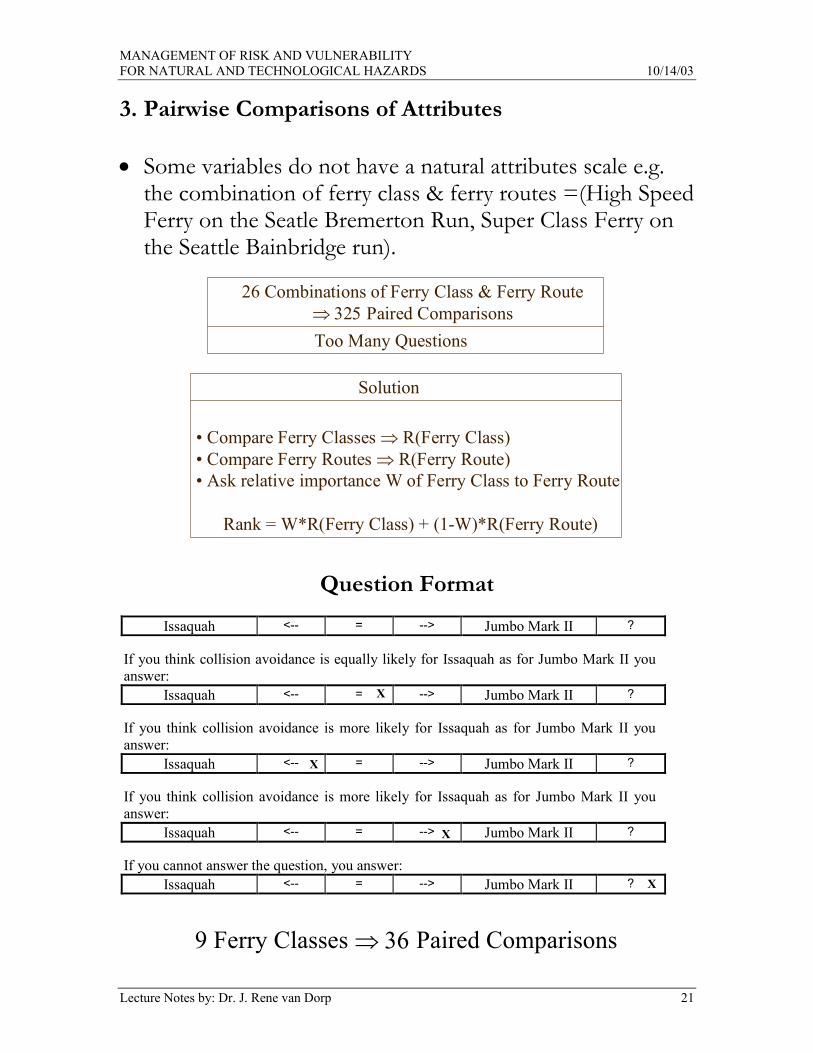
3. Pairwise Comparisons of Attributes • Some variables do not have a natural attributes scale e.g.
the combination of ferry class & ferry routes =(High Speed Ferry on the Seatle Bremerton Run, Super Class Ferry on the Seattle Bainbridge run).
26 Combinations of Ferry Class & Ferry Route⇒ 325 Paired ComparisonsToo Many Questions
Solution
• Compare Ferry Classes ⇒ R(Ferry Class)• Compare Ferry Routes ⇒ R(Ferry Route)• Ask relative importance W of Ferry Class to Ferry Route
Rank = W*R(Ferry Class) + (1-W)*R(Ferry Route)
Question Format
Issaquah <-- = --> Jumbo Mark II ?
If you think collision avoidance is equally likely for Issaquah as for Jumbo Mark II youanswer:
Issaquah <-- = --> Jumbo Mark II ?
If you think collision avoidance is more likely for Issaquah as for Jumbo Mark II youanswer:
Issaquah <-- = --> Jumbo Mark II ?
If you think collision avoidance is more likely for Issaquah as for Jumbo Mark II youanswer:
Issaquah <-- = --> Jumbo Mark II ?
If you cannot answer the question, you answer:Issaquah <-- = --> Jumbo Mark II ?
X
X
X
X
9 Ferry Classes ⇒ 36 Paired Comparisons

MANAGEMENT OF RISK AND VULNERABILITY FOR NATURAL AND TECHNOLOGICAL HAZARDS 10/14/03
Lecture Notes by: Dr. J. Rene van Dorp 22
Perform Bradley Terry Pairwise Comparison Analysis to: 1. Test for Preference Structure of individual expert by
counting circular triads. Circular Triad: A is better than B, B is better than C, C is better than A. 2. Test for Agreement between experts as a group.
Results Attribute Scale for Ferry Class
1.00
2.07
3.20
4.10
4.63
5.03
7.99
8.35
9.56
0.00 2.00 4.00 6.00 8.00 10.00 12.00
Chinook
POV
Evergreen
Issaquah
Jumbo Mark II
Steel Electric
Jumbo
Super
Rhododendron
Bra
dley
-Ter
ry S
core

MANAGEMENT OF RISK AND VULNERABILITY FOR NATURAL AND TECHNOLOGICAL HAZARDS 10/14/03
Lecture Notes by: Dr. J. Rene van Dorp 23
Results Attribute Scale for Ferry Route
1.00
1.90
2.67
4.13
7.73
24.97
27.55
27.55
43.07
52.91
82.20
92.65
0.00 10.00 20.00 30.00 40.00 50.00 60.00 70.00 80.00 90.00 100.00
MUK-CLI
PTD-TAH
SOU-VAS
FAU-VAS
FAU-SOU
EDM-KIN
SEA-VAS
PTW-KEY
ANA-SID
ANA-SJI
SEA-BAI
SEA-BRE
Bra
dley
- Te
rry
Scor
e
Using Swing Weights Elicitation Method (EMGT 269) Ferry Class Weight = 0.42 Ferry Route Weight = 0.59

MANAGEMENT OF RISK AND VULNERABILITY FOR NATURAL AND TECHNOLOGICAL HAZARDS 10/14/03
Lecture Notes by: Dr. J. Rene van Dorp 24
Results Attribute Scale for Ferry Class & Ferry Route Combination
1.00
1.08
1.27
1.29
1.37
1.45
1.64
1.76
1.84
1.85
2.03
3.08
3.14
3.60
3.66
4.04
4.17
4.32
4.43
4.86
5.28
5.30
5.80
5.82
6.15
7.36
0.00 1.00 2.00 3.00 4.00 5.00 6.00 7.00 8.00
SOU-VAS: Evergreen
FAU-VAS: Evergreen
FAU-SOU: Evergreen
MUK-CLI: Issaquah
SOU-VAS: Issaquah
FAU-VAS: Issaquah
FAU-SOU: Issaquah
SOU-VAS: Steel Electric
FAU-VAS: Steel Electric
SEA-VAS: POV
FAU-SOU: Steel Electric
PTW-KEY: Steel Electric
ANA-SID: Evergreen
PTD-TAH: Rhododendron
ANA-SJI: Evergreen
ANA-SJI: Issaquah
EDM-KIN: Jumbo
EDM-KIN: Super
ANA-SJI: Steel Electric
SEA-BRE: Chinook
ANA-SID: Super
SEA-BRE: POV
ANA-SJI: Super
SEA-BAI: Jumbo Mark II
SEA-BRE: Issaquah
SEA-BAI: Super
Com
bine
d Sc
ore
MANAGEMENT OF RISK AND VULNERABILITY FOR NATURAL AND TECHNOLOGICAL HAZARDS 10/14/03
Lecture Notes by: Dr. J. Rene van Dorp 25
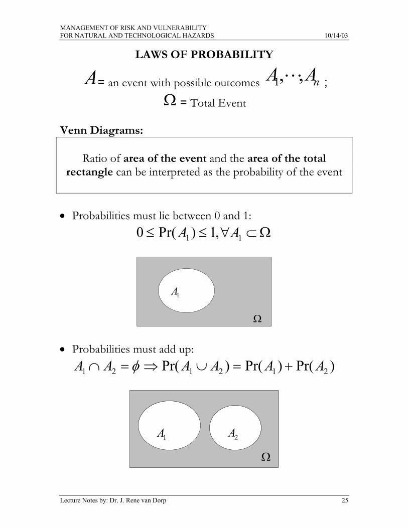
LAWS OF PROBABILITY
A= an event with possible outcomes nAA ,,1 ; Ω = Total Event
Venn Diagrams:
Ratio of area of the event and the area of the total rectangle can be interpreted as the probability of the event
• Probabilities must lie between 0 and 1: Ω⊂∀≤≤ 11 ,1)Pr(0 AA
1A
Ω
• Probabilities must add up: )Pr()Pr()Pr( 212121 AAAAAA +=∪⇒=∩ φ
1A 2A
Ω

MANAGEMENT OF RISK AND VULNERABILITY FOR NATURAL AND TECHNOLOGICAL HAZARDS 10/14/03
Lecture Notes by: Dr. J. Rene van Dorp 26
• Total Probability Must Equal 1: ( ) 1)Pr(, 3
13
1 =⇒Ω=∧≠∀=∩ == iiiiji AAjiAA ∪∪φ
1A 2A
Ω
3A
• Complement Rule: )Pr(1)Pr( 11 AA −=
1A 1A
• Probability of union of two events that can happen at the same time
)Pr()Pr()Pr()Pr( 212121 AAAAAA ∩−+=∪
1A2A
Ω

MANAGEMENT OF RISK AND VULNERABILITY FOR NATURAL AND TECHNOLOGICAL HAZARDS 10/14/03
Lecture Notes by: Dr. J. Rene van Dorp 27
Conditional Probability:
Bad Weather Car Accident
)Weather BadPr(Weather) BadAccidentCar Pr()Weather Bad|AccidentCarr Pr( ∩
=
Informally: Conditioning on an event coincides with reducing the total event to the conditioning event
• Multiplicative Rule:
)Pr()|Pr()Pr()|Pr()Pr( 11111111 BBAAABBA ∗=∗=∩
MANAGEMENT OF RISK AND VULNERABILITY FOR NATURAL AND TECHNOLOGICAL HAZARDS 10/14/03
Lecture Notes by: Dr. J. Rene van Dorp 28
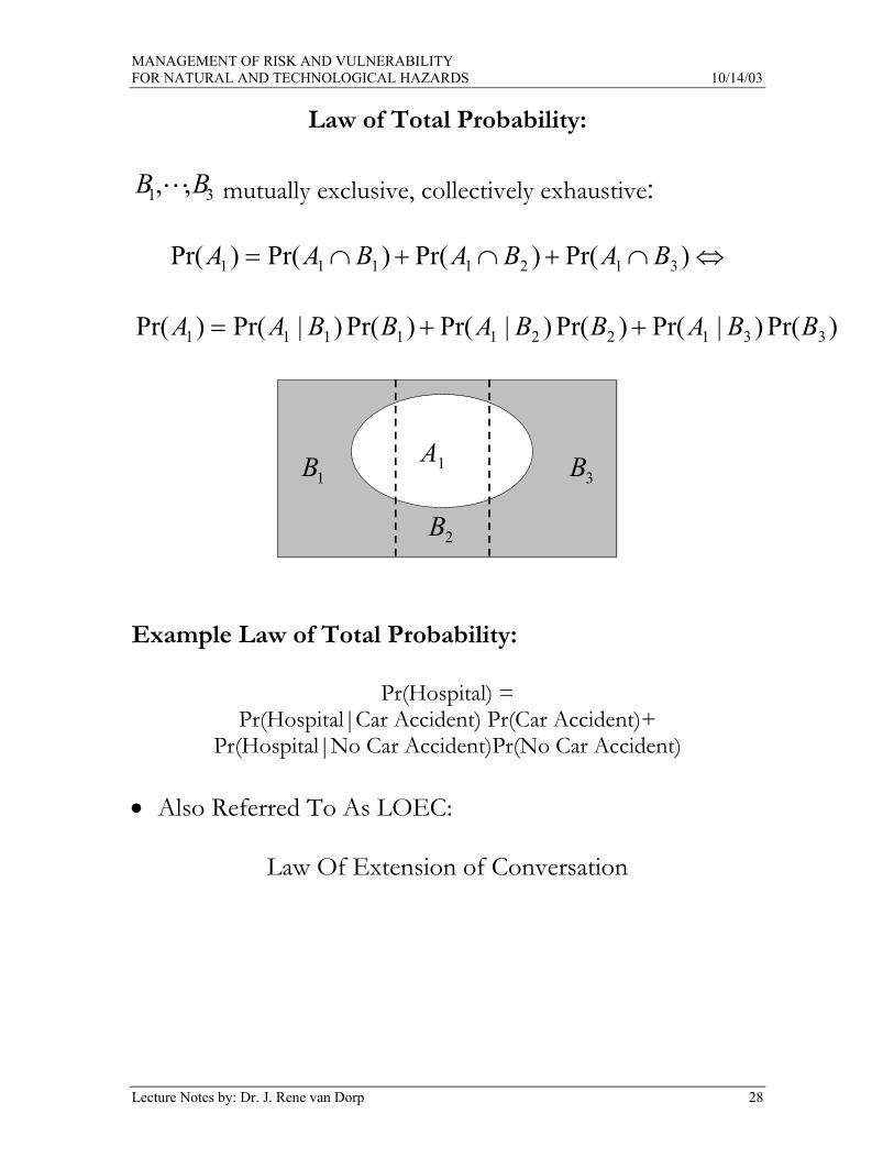
Law of Total Probability:
31 ,, BB mutually exclusive, collectively exhaustive:
⇔∩+∩+∩= )Pr()Pr()Pr()Pr( 3121111 BABABAA
)Pr()|Pr()Pr()|Pr()Pr()|Pr()Pr( 3312211111 BBABBABBAA ++=
1B
2B
3B1A
Example Law of Total Probability:
Pr(Hospital) = Pr(Hospital|Car Accident) Pr(Car Accident)+
Pr(Hospital|No Car Accident)Pr(No Car Accident) • Also Referred To As LOEC:
Law Of Extension of Conversation

MANAGEMENT OF RISK AND VULNERABILITY FOR NATURAL AND TECHNOLOGICAL HAZARDS 10/14/03
Lecture Notes by: Dr. J. Rene van Dorp 29
Bayes Theorem
31 ,, BB mutually exclusive, collectively exhaustive:
1B
2B
3B1A
)Pr()|Pr()Pr()|Pr()Pr(.1 1111 jjjj BBAAABBA ==∩
)Pr()Pr()|Pr(
)|Pr(.21
11 A
BBAAB jj
j =
)Pr()|Pr()Pr()|Pr()Pr()|Pr()Pr(.3 3312211111 BBABBABBAA ++=
)Pr()|Pr()Pr()|Pr()Pr()|Pr()Pr()|Pr(
)|Pr(.4331221111
11 BBABBABBA
BBAAB jj
j ++=

MANAGEMENT OF RISK AND VULNERABILITY FOR NATURAL AND TECHNOLOGICAL HAZARDS 10/14/03
Lecture Notes by: Dr. J. Rene van Dorp 30
Example: Game Show Suppose we have a game show host and you. There are three doors and one of them contains a prize. The game show host knows the door containing the prize but of course does not convey this information to you. He asks you to pick a door. You picked door 1 and are walking up to door 1 to open it when the game show host screams: STOP. You stop and the game show host shows door 3 which appears to be empty. Next, the game show asks.
"DO YOU WANT TO SWITCH TO DOOR 2?" WHAT SHOULD YOU DO?
Assumption 1: The game show host will never show the door with the prize. Assumption 2: The game show will never show the door that you picked. • Di =Prize is behind door i , i=1,…,3 • Hi =Host shows door i containing no prize after you
selected Door 1, i=1,…,3
Initially: 31)Pr( =iD
1. 21
31*0
31*1
31*
21)Pr()|Pr()Pr(
3
133 =++== ∑
=i
ii DDHH
2. 31
21
31*
21
)Pr()Pr()|Pr()|Pr(
3
11331 ===
HDDHHD
3. 32
311)|Pr(1)|Pr( 3132 =−=−= HDHD .
So Yes, you should switch!
MANAGEMENT OF RISK AND VULNERABILITY FOR NATURAL AND TECHNOLOGICAL HAZARDS 10/14/03
Lecture Notes by: Dr. J. Rene van Dorp 31
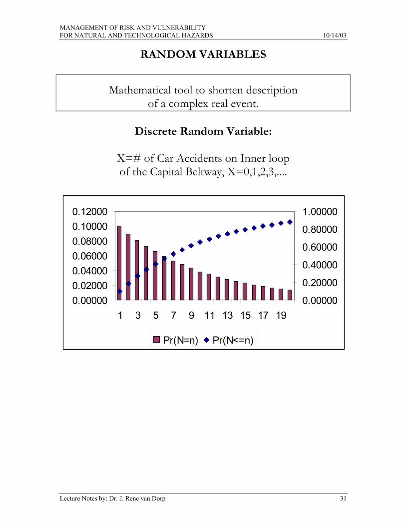
RANDOM VARIABLES
Mathematical tool to shorten description of a complex real event.
Discrete Random Variable:
X=# of Car Accidents on Inner loop of the Capital Beltway, X=0,1,2,3,....
0.000000.020000.040000.060000.080000.100000.12000
1 3 5 7 9 11 13 15 17 190.00000
0.20000
0.40000
0.60000
0.80000
1.00000
Pr(N=n) Pr(N<=n)

MANAGEMENT OF RISK AND VULNERABILITY FOR NATURAL AND TECHNOLOGICAL HAZARDS 10/14/03
Lecture Notes by: Dr. J. Rene van Dorp 32
Continuous Random Variable:
X= Failure Time of a Pressure Relief Valve under continuous pressure, X=[0, ∞
Exponential Life Time Distribution:
0.00
0.50
1.00
1.50
2.00
0.00
0.20
0.40
0.60
0.80
1.00
1.20
f(x) Pr(X<=x)
Weibull Life Time Distribution:
0.000.200.400.600.801.001.201.40
0.00
0.20
0.40
0.60
0.80
1.00
1.20
f(x) Pr(X<=x)
Failure Rate = )Pr()Pr()|Pr(
tTttTttTttTt
>∆+<<
=>∆+<<

MANAGEMENT OF RISK AND VULNERABILITY FOR NATURAL AND TECHNOLOGICAL HAZARDS 10/14/03
Lecture Notes by: Dr. J. Rene van Dorp 33
MEASURES OF CENTRAL TENDENCY
SKEWED TO LEFT : Mode < Mean < Median SKEWED TO RIGHT : Mode > Mean > Median SYMMETRIC : ?
0.00
0.50
1.00
1.50
0.000.200.400.600.801.001.20
f(x) Pr(X<=x)
Mode Median
Mean

MANAGEMENT OF RISK AND VULNERABILITY FOR NATURAL AND TECHNOLOGICAL HAZARDS 10/14/03
Lecture Notes by: Dr. J. Rene van Dorp 34
DOMINANCE AND MAKING DECISIONS UNDER UNCERTAINTY
Suppose you have to choose between two lottery tickets and the only information you have is that the expected pay-off of the first lottery ticket is lower than the second. Which one would you choose? You picked your ticket and the lotteries are played and you learn your outcome. Is your pay-off higher than the pay-off of the first lottery-ticket? Conclusion: There is a chance of an unlucky outcome. In other words there is no dominance (=deterministic dominance.
DETERMINISTIC DOMINANCE PRESENT
STOCHASTIC DOMINANCE PRESENT
CHOOSE ALTERNATIVE WITH BEST EMV
MAKING DECISIONS & RISK LEVEL
Chancesof unlucky outcomeIncreases

MANAGEMENT OF RISK AND VULNERABILITY FOR NATURAL AND TECHNOLOGICAL HAZARDS 10/14/03
Lecture Notes by: Dr. J. Rene van Dorp 35
SITUATION 1: You are given more information about both lotteries. The pay-off X of lottery 1 falls in the range from [A,B]. The pay-off from lottery 2 falls in the range from [C,D].
Assume random Variable X Uniformly Distributed on [A,B]
Assume random Variable Y Uniformly Distributed on [C,D]
DETERMINISTIC DOMINANCE
A B C D
A B C D
0
0
1
CD
F
X
YX
Y
Which one would you choose?
You picked your ticket and the lotteries are played and you learn your outcome. Is your pay-off higher than the pay-off of the first lottery-ticket? Conclusion: There is a no chance of an unlucky outcome. In other words there is dominance (=deterministic dominance).

MANAGEMENT OF RISK AND VULNERABILITY FOR NATURAL AND TECHNOLOGICAL HAZARDS 10/14/03
Lecture Notes by: Dr. J. Rene van Dorp 36
SITUATION 2: You are given more information about both lotteries. The pay-off X of lottery 1 falls in the range from [A,B]. The pay-off from lottery 2 falls in the range from [C,D].
Assume random Variable X Uniformly Distributed on [A,B]
Assume random Variable Y Uniformly Distributed on [C,D]
STOCHASTIC DOMINANCE
A BC D
A BC D
0
0
1
CD
F
Pr(Y<z) < Pr(X< z) Note:
for all z
X
X
Y
Y
You picked your ticket and the lotteries are played and you learn your outcome. Is your pay-off higher than the pay-off of the first lottery-ticket? Conclusion: There is a a chance of an unlucky outcome. In this case there is stochastic dominance, but no deterministic dominance.

MANAGEMENT OF RISK AND VULNERABILITY FOR NATURAL AND TECHNOLOGICAL HAZARDS 10/14/03
Lecture Notes by: Dr. J. Rene van Dorp 37
SITUATION 3: You are given more information about both lotteries. The pay-off X of lottery 1 falls in the range from [A,B]. The pay-off from lottery 2 falls in the range from [C,D].
Assume random Variable X Uniformly Distributed on [A,B]
Assume random Variable Y Uniformly Distributed on [C,D]
CHOOSE ALTERNATIVE WITH BEST EMV
A BC D
A BC D
0
0
1
CD
F
X
YX
Y
E(Y)E(X)
You picked your ticket and the lotteries are played and you learn your outcome. Is your pay-off higher than the pay-off of the first lottery ticket?

MANAGEMENT OF RISK AND VULNERABILITY FOR NATURAL AND TECHNOLOGICAL HAZARDS 10/14/03
Lecture Notes by: Dr. J. Rene van Dorp 38
UNCERTAINTY ANALYSIS VERSUS SENSITIVITY ANALYSIS
MODEL =F(X,Y,Z)
0.00
0.50
1.00
1.50
2.00
2.50
3.00
3.50
0.00 0.20 0.40 0.60 0.80 1.00
0.00
0.50
1.00
1.50
2.00
2.50
3.00
3.50
0.00 0.20 0.40 0.60 0.80 1.00
0.00
0.20
0.40
0.60
0.80
1.00
1.20
1.40
0.00 0.20 0.40 0.60 0.80 1.00
INPUT UNCERTAINTY
OUTPUT
0.00
0.50
1.00
1.50
2.00
2.50
0.00 0.20 0.40 0.60 0.80 1.00
L UM
UM
UML
L
Uncertainty Analysis = Quantificationof Output Uncertainty given Modeland Input Uncertainty
Sensitivity Analysis = Sensitivity ofOutput Parameter to change in oneparameter keeping others constant.
MS1
X
Y
Z

MANAGEMENT OF RISK AND VULNERABILITY FOR NATURAL AND TECHNOLOGICAL HAZARDS 10/14/03
Lecture Notes by: Dr. J. Rene van Dorp 39
MONTE CARLO SIMULATION
MODEL =F(X,Y,Z)
0.00
0.50
1.00
1.50
2.00
2.50
3.00
3.50
0.00 0.20 0.40 0.60 0.80 1.00
0.00
0.50
1.00
1.50
2.00
2.50
3.00
3.50
0.00 0.20 0.40 0.60 0.80 1.00
0.00
0.20
0.40
0.60
0.80
1.00
1.20
1.40
0.00 0.20 0.40 0.60 0.80 1.00
INPUT UNCERTAINTY
OUTPUT
0.00
0.50
1.00
1.50
2.00
2.50
0.00 0.20 0.40 0.60 0.80 1.00
X
Y
Z
Sample X1,Y1,Z1 O1
O
Calculate
Sample X2,Y2,Z2 O2Calculate
Sample X3,Y3,Z3 O3Calculate
STA
TIST IC
S
ETC ...

MANAGEMENT OF RISK AND VULNERABILITY FOR NATURAL AND TECHNOLOGICAL HAZARDS 10/14/03
Lecture Notes by: Dr. J. Rene van Dorp 40
REGRESSION ANALYSIS
MODEL:O = a1(X)+a2G(Y)+a3H(Z)
INPUT UNCERTAINTY
OUTPUT
G(Y)
H(Z)
O
0.00
0.50
1.00
1.50
2.00
2.50
3.00
3.50
0 .00 0.20 0 .40 0.60 0 .80 1.00
0.00
0.50
1.00
1.50
2.00
2.50
3.00
3.50
0.00 0.20 0.40 0.60 0.80 1.00
0.00
0.50
1.00
1.50
2.00
2.50
0.00 0.20 0.40 0.60 0.80 1.00
Data on X
Data on Y
DATA on Z
IndependentVariables
Assumption 1:Normality
Assumption
0.00
0.50
1.00
1.50
2.00
2.50
Assumption 2:Linearity
Assumption
0.00
0.10
0.20
0.30
0.40
0.50
0.60
F(X)
0 .00
0 .50
1 .00
1 .50
2 .00
2 .50
0.00
0.50
1.00
1.50
2.00
2.50


