EMGT 835 FIELD PROJECT - KU ScholarWorks - The University of
EMGT 835 FIELD PROJECT: Improving Inventory Control Using Forecasting
By
Juan Mario Balandran [email protected]
Master of Science
The University of Kansas
Fall Semester, 2005
An EMGT Field Project report submitted to the Engineering Management Program and the Faculty of the Graduate School of The University of Kansas in partial fulfillment of the
requirements for the degree of Master of Science.
______________________________ Zerwekh, Robert P., Ph.D. Date Committee Chair
______________________________ Bowlin, Tom, Ph.D. Date Committee Member
______________________________ Keller, Charles W., MBA Date Committee Member

Forecasting Product Demand for Electronics Controls, Inc 1
Acknowledgments
This project could not have been successful without the love and support of my wife, Tanya
and my parents, Mario and Martha. Thanks also to Dr. Tom Bowlin (my “guide”), Dr. Zerwekh and
Dr. Keller for their knowledge and encouragement.
I am very grateful to Lucille and Michael Hobbs for their friendship, understanding and
financial support. Finally, thank you to Tom Decker, Pat Jackson and Brian Zellar for all their
contributions and hard work on this project.

Forecasting Product Demand for Electronics Controls, Inc 2
Executive Summary
This project studied and analyzed Electronic Controls, Inc.’s forecasting process for three high-
demand products. In addition, alternative forecasting methods were developed to compare to the
current forecast method. The following is a list of the main findings:
• The three selected products showed a prominent irregular component.
• The optimal forecasting method for each product was different.
• The current forecasting method produced unacceptable forecasts for two of the selected
products.
• Two of the model-based forecasts were more accurate than the forecast produced by
the current process.
The following are the main recommendations to improve the current forecasting process:
• Electronic Controls should keep track of the sales data instead of the shipping data to
forecast the demand of each product.
• Electronic Controls should keep track of the forecasting error in order to calculate the
accuracy measures.
• Implementing the tracking signal for the forecast of each product will improve the
accuracy of the current forecasting process.

Forecasting Product Demand for Electronics Controls, Inc 3
Table of Contents
Acknowledgments ....................................................................................................................................0
Executive Summary..................................................................................................................................2
Table of Contents .....................................................................................................................................3
Index Table ................................................................................................................................................5
Table of Figures ........................................................................................................................................7
Introduction...............................................................................................................................................8
Literature Review......................................................................................................................................9
Methodology............................................................................................................................................10
Current Inventory Forecast Process ...........................................................................................10
Development of Alternative Forecast Process..........................................................................10
Current and Alternative Forecast Process Comparison...........................................................19
Results.......................................................................................................................................................20
Current Inventory Forecast Process ...........................................................................................20
Model-Based Forecast Process ....................................................................................................25

Forecasting Product Demand for Electronics Controls, Inc 4
Evaluation of Forecasting Process: Model-Based Vs Judgmental Forecast .........................46
Conclusions and Recommendations....................................................................................................49
Suggestions for Additional Work .........................................................................................................52
References / Bibliography.....................................................................................................................54
APPENDIX A........................................................................................................................................56

Forecasting Product Demand for Electronics Controls, Inc 5
Index
Table 1 - Inventory Planning Report ............................................................................................................21
Table 2 - Sales Analysis Sheet for the OE331 .............................................................................................23
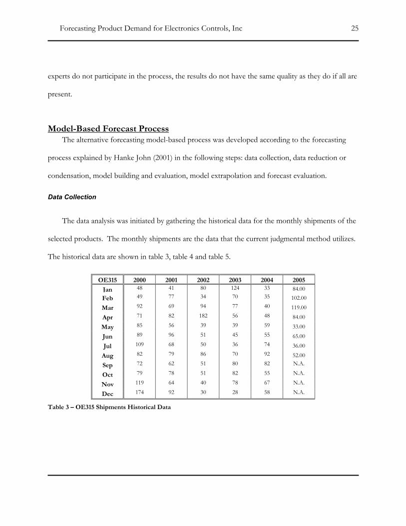
Table 3 – OE315 Shipments Historical Data ..............................................................................................25
Table 4 - OE320 Historical Data...................................................................................................................26
Table 5 - OE331 Historical ............................................................................................................................26
Table 6- Adjusted OE315 Data .....................................................................................................................29
Table 7- Adjusted OE320 Data .....................................................................................................................30
Table 8 - Adjusted OE331 Data....................................................................................................................31
Table 9- Results from Model-Base Forecasting Methods for the OE315 ..............................................37
Table 10 - Results from the Trend Forecasting Methods for the OE320...............................................38
Table 11 - Results from the Trend Forecasting Methods for the OE331...............................................38
Table 12 - OE315 Forecast for 2005 ............................................................................................................39
Table 13 - OE320 Forecast for 2005 ............................................................................................................40
Table 14 - OE331 Forecast for 2005 ............................................................................................................40

Forecasting Product Demand for Electronics Controls, Inc 6
Table 15 - Accuracy Measures for OE315 Forecast (2005) ......................................................................41
Table 16 - Accuracy Measures for OE320 Forecast (2005) ......................................................................42
Table 17 - Accuracy Measures for OE331 Forecast (2005) ......................................................................43
Table 18 - Forecast and Accuracy Measures for the OE320 12 Month Linear Regression .................44
Table 19 - Forecast and Accuracy Measures for the OE331 12 Months Linear Regression................45
Table 20 – Forecasted Values and Accuracy Measures for OE315 .........................................................46
Table 21 – Forecasted Values and Accuracy Measures for OE320 .........................................................47
Table 22– Forecasted Values and Accuracy Measures for OE331 ..........................................................48

Forecasting Product Demand for Electronics Controls, Inc 7
Table of Figures
Figure 1 – Scatter Diagram for the OE315 Historical Data......................................................................27
Figure 2 - Scatter Diagram for the OE320 Historical Data.......................................................................27
Figure 3 - Scatter Diagram for the OE331 Historical Data.......................................................................28
Figure 4 - Scatter Diagram for the OE315 Adjusted Data........................................................................32
Figure 5 - Scatter Diagram for the OE320Adjusted Data .........................................................................32
Figure 6 - Scatter Diagram for the OE331 Adjusted Data........................................................................33
Figure 7 - Autocorrelation Analysis for the OE315 Adjusted Data.........................................................34
Figure 8 - Autocorrelation Analysis for the OE320 Adjusted Data.........................................................35
Figure 9 - Autocorrelation for the OE331 Adjusted Data ........................................................................36

Forecasting Product Demand for Electronics Controls, Inc 8
Introduction
Electronic Controls, Inc. is a privately owned company located in Kansas City, Missouri, which
develops innovative control solutions for the building automation industry. Inventory is an essential
component of this company and can greatly effect its financial situation.
Currently, the company calculates its inventory level based on a judgmental forecasting process.
Judgmental forecasting is built around the idea that the knowledge and intuition of the company’s
experts are the best tools to forecast the future demand of products. While this method has been
working satisfactorily, no forecasting process is perfect. It is in Electronic Control’s best interest to
investigate the accuracy of the current process and whether or not there are more effective
alternatives to be applied.
Statistical and forecasting theories will be studied and applied to achieve these main goals:
• Study and understand the current Electronic Controls forecasting process
• Evaluate the accuracy of the current forecasting process
• Develop alternative forecasting methods
• Compare the current and alternative forecasting methods
• Recommend ways to make the forecast more accurate
Electronic Controls’ management will be presented with the results of this investigation. They
can then take the appropriate measures to improve forecasting.

Forecasting Product Demand for Electronics Controls, Inc 9
Literature Review
The main component of this project required research in time series forecast theory. That
research encompassed the following areas: comprehension and identification of the time series
components, understanding and application of different forecasting methods and evaluation of the
forecasting results. The following titles cover the above-mentioned topics in detail:
1. Bowerman, Bruce L., Richard T. O’Connell and Anne B. Koehler. 2005. Forecasting,
Time Series, and Regression.
2. Hanke, John E. Dean W. Wichern and Arthur G. Reitsch. 2001. Business Forecasting.
A Companion to Economic Forecasting by the editors Michael P. Clements and David F. Hendry has
a chapter dedicated to judgmental forecasting. This chapter discusses the format and the strengths
and weaknesses of judgmental forecasting. In addition, it compares judgmental and model-based
forecasts.
The books listed below are dedicated to the study of inventory management and the application
of forecasting in the inventory management process. Of special interest was the study of areas that
explain the process of modeling the product demand accurately and of learning the forecasting
methods that are most widely implemented by other companies.
1. Axsäter, Sven. 2000. Inventory Control.
2. Toomey, John W. 2000. Inventory Management: Principles, Concepts and Techniques.
3. Seth, Suresh P., Houmin Yan and Hanqin Zhang. 2005. Inventories and Supply Chain
Management with Forecast Updates.

Forecasting Product Demand for Electronics Controls, Inc 10
Methodology
The explanation of research required in the project is divided into three main sections. The first
section is the explanation of research required to understand the current inventory forecast process.
The second section concerns development of a preferred alternative forecast method. The last
section addresses and analyzes the comparisons made between the results of the current forecast
process and those of the studied alternative forecasting methods.
Current Inventory Forecast Process To understand how the current inventory forecast method works, interviews were performed to
supplement information available from personal experience. The interviewees included personnel
from the management, accounting and production departments. The personal experience was
gained through direct observation of business meetings and other interactions that the personnel in
charge of forecasting had during the last two months. The business meetings attended included only
those related to the current forecasting method.
Development of Alternative Forecast Process Electronics Controls’ executives selected three products for which to develop alternative
model-based forecasts. The products were selected because they are considered high-demand
products. They are the OE315, the OE320 and the OE331. The alternative forecasting model-
based process was developed according to the forecasting process explained by Hanke John (2001)
in the following steps:

Forecasting Product Demand for Electronics Controls, Inc 11
1. Data Collection
2. Data Reduction or Condensation
3. Model Building and Evaluation
4. Model Extrapolation
5. Forecast Evaluation
For the data collection step, it is important to collect the proper data and to verify that the
data are correct. Ideally, sales data are used to develop the forecast of a product’s demand.
Unfortunately, Electronic Controls does not keep track of this data. Thus, the amount of products
shipped was used instead to forecast the demand for the three selected products. Electronic
Controls receives the three selected products monthly, therefore, shipments data were also recorded
monthly.
For the data reduction or condensation step, data that are not relevant to the problem at
hand are eliminated to make the data more representative and thus improve the accuracy of the
forecast. Shipment data were collected from January 2000 until August of 2005. Any previous data
were removed from the analysis because shipments for the three selected products did not become
consistent until the year 2000. Several authors advise against using the shipping data instead of sales
data to forecast the future demand (Axsater 2000, Toomey 2000 and Sethi 2005). The main reason
behind this is that shipping information could include late or incomplete orders that could reduce
the accuracy of the forecast. In an effort to adjust the shipping data to more accurately resemble
sales data, historical shipping records were analyzed to identify data points at which late or

Forecasting Product Demand for Electronics Controls, Inc 12
incomplete orders occurred. The identified data points were then adjusted in order to reflect sales as
opposed to shipping data. Other modifications were made to the data to eliminate once in a lifetime
events that did not reflected the normal demand of the products.
In the model building and evaluation step, a forecasting method is selected based on its
ability to minimize forecasting error and on the expected ease of implementation. Highly
sophisticated methods may be more accurate, but they are more complicated to put into action. In
most cases, balance needs to be found between sophistication and accuracy.
The shipping data for each product were divided into two sets, one set being from the years
2000 to 2004 and the other set including only data from 2005. The 2000-2004 data set was used
only to fit the different parameters of the studied forecasting methods. The 2005 data set was used
to test the accuracy of the forecasting methods.
The 2000-2004 data sets for the different products were analyzed to identify which of the
following components were present:
1. Trend is the component that represents the underlying sustained growth or decline in
the data.
2. Seasonal components are typically found in quarterly, monthly or weekly data.
Seasonal variations refer to stable patterns of change that appear and repeat over some
time frame.
3. Cyclical components are a series of wavelike fluctuations in data of more than one
year’s duration.
4. The irregular component consists of unpredictable or random fluctuations.

Forecasting Product Demand for Electronics Controls, Inc 13
The tools applied to identify the different components in the 2000-2004 data sets were the
scatter diagram and autocorrelation analysis:
• Scatter diagrams plot the shipments-time points on a two-dimensional graph (Hanke
2001). The diagrams help to illustrate any patterns in the data and, at the same time,
identify the components that created the patterns.
• Autocorrelation is the correlation between a variable lagged one or more periods and
itself (Hanke 2001). In autocorrelation analysis, the patterns in autocorrelation
coefficients for different time lags are studied to identify data components.
Another important aspect that can be studied from autocorrelation analyses is whether or not
the time series data being analyzed can be characterized as random. The Ljung and Box Q (LBQ)
statistic was applied to test if the 2000-2004 data sets could be considered random. The Q statistic
is derived through the equation
Q = n (n +2) Σk= 1 to m (r k 2)/(n-k).
Where:
• n is the number of observations in the time series.
• k is the time lag.
• m is the number of time lags to be tested.
• r k is the sample autocorrelation function of the residuals lagged k time periods.
This test assumes that Q statistics from autocorrelation of a time series follow a Chi-square
distribution with the degrees of freedom equal to m minus the number of parameters to be estimated

Forecasting Product Demand for Electronics Controls, Inc 14
in the model (Hanke 2001). MINITAB statistical software was employed to calculate the LBQ
statistic values for autocorrelation analyses for the three selected products.
After the different components in the data were identified, reasonable forecasting methods
were selected and applied to create forecasts for the three selected products. The methods were
then evaluated to determine which were more accurate. The methods evaluated are shown below:
1. Naïve
2. Linear Regression
3. Moving Average
4. Exponential
5. Double exponential
The naïve forecasting method assumes that more recent data values are the best predictors of
future values. The model is Ŷt+1 = Yt . Where Ŷt+1 is the forecast made at time t for the time t+1.
This forecast method disregards all of the earlier observations and, because of that, it tracks changes
quickly.
The linear regression forecasting method produces the line that best fits a collection of X-Y
points. The linear regression fitted line follows the model Ŷ = b0 + b1X, where Ŷ is a calculated Y
value for a given X value, b0 is the intercept and b1 is the slope of the line. The parameters to be
calculated for this method were the b0 and b1 values. The b0 and b1 values were determined from the
2000-2004 data sets and the application of the MINITAB software package. MINITAB uses the

Forecasting Product Demand for Electronics Controls, Inc 15
method of least squared errors to determine the best fitted line and the respective b0 and b1 values for
the 2000-2004 data sets.
The moving average forecasting method uses the average of a constant number of most
recent data points. As new values become available, the moving average includes the latest value
and discards the oldest value. The moving average follows the model: Ŷt+1 = (Yt + Yt-1 + … + Yt-
k+1)/k. Where Ŷt+1 is the forecast made for the next data point, Yt is the value at period t and k are
the number of terms in the moving average. The parameter to be calculated for this method was the
k value. The k value was determined by using the 2000-2004 data sets and the application of
MINITAB software package to manually calculate accuracy for the k values from one to twelve.
The most accurate k value was the one selected.
The simple exponential method provides an exponentially weighted moving average of all the
previous data points. The simple exponential method follows the model Ŷt+1 = αYt + (1 - α) Ŷt..
Where Ŷt+1 is the forecast made for the next data point, Yt is the value at period t, Ŷt is the old
forecast for period t and α is the smoothing constant (0 < α < 1). The parameter to be calculated
for this method was the α value. The α value was determined by using the 2000-2004 data sets and
the application of the MINITAB software package to calculate the α value that provided the most
accurate forecast. MINITAB automatically selects the α by fitting the entire range of possible values
to the equation and selecting the α that minimizes the sum of squared errors.
The double exponential method provides an exponentially weighted moving average of all the
previous data points and allows for evolving local trends in a time series. The double exponential

Forecasting Product Demand for Electronics Controls, Inc 16
method uses different constants to directly smooth the level and the slope. The three equations that
model the double exponential method are:
• The exponentially smoothed series: Lt = αYt + (1 - α) (Lt-1. + T t-1)
• The trend estimate: T t = β((Lt. - L t-1) + (1 - β) T t-1
• Forecast p period of time into the future: Ŷt+p = Lt + p T t
Where:
• Ŷt+p is the forecast made p periods into the future.
• Yt is the actual value at period t.
• α is the smoothing constant (0 < α < 1).
• Lt is the newly smoothed value.
• β is the smoothing constant for the trend (0 < β < 1).
• T t is the trend estimate.
• p is the periods to be forecast into the future.
• Ŷt+p is the forecast for p periods into the future.
The parameters to be calculated for this method were the α and β values. The α and β values
were determined by using the 2000-2004 data sets and the application of the MINITAB software

Forecasting Product Demand for Electronics Controls, Inc 17
package to calculate the α and β values that gave the most accurate forecast. MINITAB selects the
α and β by fitting the entire range of possible values for both variables to the equations and
selecting the α and β that minimize the sum of squared errors.
The various methods applied to evaluate the accuracy of the different forecasting methods are
explained below.
• Mean Absolute Percentage Error (MAPE): measures the accuracy of forecasted time
series values. It expresses accuracy as a percentage and provides an idea of how large the
magnitude of the errors is compared to the actual values.
MAPE = (1/n) * Σt = 0 to n (|Yt – Ŷt|/ Yt) and Yt ≠ 0.
Where Yt is the actual value at time t, Ŷt is the forecasted value for time t and n is the
number of observations. (From MINITAB software package, help files).
• Mean Absolute Deviation (MAD): measures the accuracy of forecasted time series values.
It expresses accuracy in the same units as the data, which helps conceptualize the amount of
error.
MAD = (1/n) * Σt = 0 to n (|Yt – Ŷt|).
Where Yt is the actual value at time t, Ŷt is the forecast value for time t and n is the number
of observations. (From MINITAB software package, help files).

Forecasting Product Demand for Electronics Controls, Inc 18
• Mean Squared Deviation (MSD): measures the accuracy of forecasted time series values.
Like the MAD, it expresses accuracy in the same units as the data, but it is a more sensitive
measure of unusually large forecast errors than MAD.
MSD = (1/n) * Σt = 0 to n (|Yt – Ŷt|) 2.
Where Yt is the actual value at time t, Ŷt is the forecast value for time t and n is the number
of observations. (From MINITAB software package, help files).
• Mean Percentage Error (MPE): expresses accuracy as a percentage and provides an idea
if the forecast is consistently overestimating or underestimating values.
MPE = (1/n) * Σt = 0 to n ((Yt – Ŷt)/ Yt) and Yt ≠ 0.
Where Yt is the actual value at time t, Ŷt is the forecast value for time t and n is the number
of observations. (Hanke, John 2001).
In the Model Extrapolation step, the monthly forecast for 2005 was generated. The two
methods that gave the best accuracy measures for each product for the 2000-2004 data sets were
applied to forecast the 2005 points. The same parameters used to fit the forecasting methods to the
2000-2004 data sets were used to create the 2005 forecast. Only the points from January to August
2005 were included in the forecast because data from the remaining months did not yet exist.
In the Forecast Evaluation step, the forecasted values were compared to the historical values.
The accuracy of the methods was also compared to alternative forecasting methods to select the one

Forecasting Product Demand for Electronics Controls, Inc 19
that best fit the application. The forecasting errors were analyzed in order to see if the parameters in
the method needed to be modified or fine-tuned. The 2005 data sets were used in the analysis.
The tool that was used to evaluate whether or not the parameters calculated from the 2000-2004
data sets are still appropriate to perform the 2005 monthly forecast was the tracking signal. The
tracking signal used in this research is a ratio that compares the cumulative sum of errors to MAD
(Bowerman, 2005). It is derived through the formula:
Tracking Signal = (Σt = 0 to n (Yt – Ŷt))/MAD.
Where Yt is the actual value at time t, Ŷt is the forecast value for time t and n is the number of
observations. Accurate forecasting methods should produce the same amount of positive and
negative errors, creating a tracking signal close to zero. A tracking signal above ±5 (level
recommended by Toomey, 2000) indicates that the forecast is constantly over or underestimating
the real value, and thus the forecasting error is larger than an accurate forecasting method could
reasonably produce.
Current and Alternative Forecast Process Comparison While the present judgmental forecasting process has been useful for the company, it has never
been compared to other forecasting processes. No forecasting process is perfect, but it is important
for any company to investigate, in the very least, the accuracy of its forecasting process. Before
starting the comparison, the forecast used in the current process was recreated from Electronic
Controls’ historical records. Then, the current forecast for each product was compared to the
alternative process forecasts developed in the previous section. Finally, observations were recorded
and the best forecasting process was selected for each product.

Forecasting Product Demand for Electronics Controls, Inc 20
Results
Current Inventory Forecast Process Electronic Controls experts participate in a forecasting meeting held the first week of each
month to study the status of Electronic Controls’ inventory and to generate forecasts for the
different products in inventory. In the meeting, experts analyze two documents to make decisions
about inventory levels. The documents are the Sales Analysis Sheet (SAS) and the Inventory
Planning Report (IPR). The SAS contains information about the previous shipping information
including the average of the last 3, 6 and 12 months. It also includes the total shipments for the last
3, 6 and 12 months as well as the maximum amount of shipments in the last 12 months. Table 2
shows an example of the SAS for the product OE331. Electronic Controls’ experts study the SAS
as a foundation to calculate the future demand forecasts. The IPR has the information about
Electronics Controls’ products, their current inventory status and current orders. Table 1 shows an
example of the IPR for the product OE331. The most important information from the IPR is the
“Assy at Vendor” (Assembly at Vendor) and the “Min on Hand” (Minimum on Hand) values for
each product.
The “Assy at Vendor” value, or lot size, is the amount of the product received each desired
period, in this case monthly, from the supplier(s). At the same time, the lot size is also the
forecasted amount to be sold during that same period. For the OE331 the lot size is 300 units per
month. Selecting or adjusting the “Assy at Vendor” value is the main goal of the monthly
forecasting meetings.

Forecasting Product Demand for Electronics Controls, Inc 21
The “Min on Hand” value is the safety stock quantity and is assigned during the monthly
forecasting meetings. Safety stock is a given amount of extra inventory set aside to protect against
fluctuations in demand or supply (Toomey 2000). Upper management, using expert opinion, assign
these values with the goal of maintaining the lowest inventory level possible while still servicing
customers efficiently. For the OE331 the “Min on Hand” value is 200 units. The “Min on Hand”
value is important to the forecasting process because it is included in some of the rules followed by
the company’s experts to assign or adjust the “Assy at Vendor” value.
Part Number Description On Order
STOCK Assy at Vendor Work Order
Number
WIP Notes Min on
Hnd
Re-order Qty
OE331 Total OE331 362 424 300/ mo OEM & Suntron
Ave: 278, Max 411
200 200
OE331-AT TUC-5R PLUS ASS'Y & TEST
205
OE331-21-AAON CONTROLLER, TUC-5R+ AAON
P/N# R20700
350 200 200 = Release quantity
OE331-21-CUSTOM TUC-5R PLUS W/BACKPLATE, CUSTOM CODE
3
OE331-21-DM DEMAND MONITOR
CONTROLLER
1
OE331-21-DS TUC-5R PLUS W/BACKPLATE
OE331-21-GPCPLUS
GENERAL PURPOSE
CONTROLLER PLUS (TUC5R+)
5 3 Planned Will advise
OE331-21-HCCO HCCO CONTROLLER
BOARD
OE331-21-MUA MUA CONTROLLER
BOARD
4 Planned Ave: 6, Max 12 5 10
Table 1 - Inventory Planning Report

Forecasting Product Demand for Electronics Controls, Inc 22
The following are the rules management use to generate “Assy at Vendor” values:
1. The lot size for the three selected products for this study (OE315, OE 320 and OE331)
can only be changed every 4 months because these products are complex and it takes time
for the suppliers to change their production lines.
2. The company’s experts use the shipping averages of the last three, six and twelve months
from the SAS to assign the lot size. The averages are studied to detect any trends in the
monthly shipments. If a trend is detected, the experts use the average of the last three
months and adjust the average to reflect the magnitude and direction of the trend. For
example, the average numbers for the OE331 were 278, 275 and 261. Because an upward
trend is detected, 300 is selected as the lot size. The amount the average is adjusted
depends on the experience and knowledge of the experts. If no trend is detected, the
experts usually round the average for the last three-months up or down. Table 2 shows
the Sales Analysis Sheet for the OE331.
3. The “Assy at Vendor” value is decreased if the inventory level runs above the “Min on
Hand” value plus the “Assy at Vendor” value for three to six months in a row. In the
case of the OE331, the inventory level would have to be constantly above 500 units, as
the “Min on Hand” value is 200 and the “Assy at Vendor” value is 300, in order for the
“Assy at Vendor” value to be decreased.
4. In some cases, management asks the supplier to delay a shipment instead of decreasing
the lot size until inventory reaches normal levels. This method is used depending on the
suppliers’ preference and their ability to change their production lines.

Forecasting Product Demand for Electronics Controls, Inc 23
5. The “Assy at Vendor” value is increased if the inventory level runs below the “Min on
Hand” value number for three to six months in a row. In the case of the OE331, the
inventory level would have to be constantly below 200 to increase the “Assy at Vendor”.
6. If the inventory level runs below the “Min on Hand” value, but management do not
believe it is a trend, then an extraordinary order is made for the amount of units
management believes could restore balance to the inventory.
7. The “Assy at Vendor” can also be adjusted in any direction if the experts in the company
predict that external factors may increase or decrease demand for a certain product.
Averages Totals Maximum
Part Number Unit Name 3 mo. 6 mo. 12 mo. 3 mo. 6 mo. 12 mo. Month
OE331 TOTAL 278 275 261 835 1,648 3,134 411
OE331-21 TUC-5R PLUS MOUNTED ON
BACKPLATE 2 1 14 5 8 172 152
OE331-21-AAON CONTROLLER, TUC-5R+ AAON
P/N# R20700 215 222 207 645 1,330 2,483 350
OE331-21-CUSTOM TUC-5R PLUS W/BACKPLATE,
CUSTOM CODE 2 6 3 7 34 40 25 OE331-21-DS TUC-5R PLUS W/BACKPLATE 1 1 3 7 4
OE331-21-GPCPLUS GENERAL PURPOSE
CONTROLLER PLUS (TUC5R+) 8 4 2 23 26 26 11 OE331-21-MUA MUA CONTROLLER BOARD 6 6 6 19 34 66 12
MG746-CAV CAV CONTROLLER PACKAGE 1 1 1 1 MG750-VAV VAV CONTROLLER PACKAGE 2 1 1 6 6 11 5
OE747 CV-C CONTROLLER PACKAGE 14 10 6 43 62 74 40 Table 2 - Sales Analysis Sheet for the OE331
While the three, six and twelve month averages are used in the current forecasting process, the
final decision is highly influenced by the instinct and knowledge of the experts present at the
meeting. Because of this, the forecasting process can be classified as judgmental forecasting.
Judgmental forecasting focuses on the incorporation of forecasters’ opinions and experiences into

Forecasting Product Demand for Electronics Controls, Inc 24
the prediction process (Clements and Hendry 2002). Electronic Controls’ experts prefer this
method because it is simple and few data need to be prepared before the meeting. Simplicity is
especially important in a small company like Electronic Controls, as the experts have many roles and
cannot dedicate large amounts of time to the forecasting process. Another factor in the preference
of these kinds of forecasting methods is that small companies do not have the resources or structure
to gather the necessary data required to build an accurate model-based forecast.
While Judgmental Forecasting is widely used in industry and it has provided advantages in
certain situations, it is not without its weaknesses. Clements and Hendry (2002) mention the
following factors that affect the accuracy of this kind of forecasting:
• The format in which the data are presented influences the forecast. Graphical
presentation is generally superior to tabular, with the exception of long-term forecasts in
series with high noise.
• Judgmental forecasting can be influenced by the biased decisions of the forecaster.
Examples of the relevant biases in forecasting include: illusory correlation (false beliefs
regarding the relativity of certain variables), selective perception (discounting
information on the basis of its inconsistency with the forecaster’s beliefs),
underestimating uncertainty, optimism and overconfidence. (Clements and Hendry
2002).
Another weakness that can be observed in Electronics Controls is that the accuracy of the
forecast depends mainly on the knowledge of few members of the forecasting team. If any of the
Forecasting Product Demand for Electronics Controls, Inc 25
experts do not participate in the process, the results do not have the same quality as they do if all are
present.
Model-Based Forecast Process The alternative forecasting model-based process was developed according to the forecasting
process explained by Hanke John (2001) in the following steps: data collection, data reduction or
condensation, model building and evaluation, model extrapolation and forecast evaluation.
Data Collection
The data analysis was initiated by gathering the historical data for the monthly shipments of the
selected products. The monthly shipments are the data that the current judgmental method utilizes.
The historical data are shown in table 3, table 4 and table 5.
OE315 2000 2001 2002 2003 2004 2005
Jan 48 41 80 124 33 84.00 Feb 49 77 34 70 35 102.00
Mar 92 69 94 77 40 119.00
Apr 71 82 182 56 48 84.00
May 85 56 39 39 59 33.00
Jun 89 96 51 45 55 65.00
Jul 109 68 50 36 74 36.00
Aug 82 79 86 70 92 52.00
Sep 72 62 51 80 82 N.A.
Oct 79 78 51 82 55 N.A.
Nov 119 64 40 78 67 N.A.
Dec 174 92 30 28 58 N.A.
Table 3 – OE315 Shipments Historical Data

Forecasting Product Demand for Electronics Controls, Inc 26
OE320 2000 2001 2002 2003 2004 2005
Jan 265 467 360 265 136 337.00 Feb 302 354 451 399 222 397.00 Mar 583 406 453 305 283 543.00 Apr 369 497 620 279 364 560.00 May 694 415 310 308 262 378.00 Jun 669 330 286 515 360 309.00 Jul 463 645 419 275 335 417.00
Aug 603 477 355 374 380 663.00 Sep 509 385 265 448 447 N.A.
Oct 534 589 648 388 239 N.A.
Nov 592 270 299 326 361 N.A.
Dec 1208 462 344 211 559 N.A.
Table 4 - OE320 Historical Data
OE331 2000 2001 2002 2003 2004 2005
Jan 60 106 161 177 113 217.00 Feb 163 110 15 178 134 185.00
Mar 404 204 177 233 134 411.00
Apr 132 155 365 252 131 289.00
May 94 112 179 278 226 277.00
Jun 124 176 180 198 388 269.00
Jul 139 135 160 226 291 257.00
Aug 211 245 145 207 251 446.00
Sep 195 116 106 81 225 N.A.
Oct 81 219 133 47 227 N.A.
Nov 182 269 133 238 264 N.A.
Dec 205 165 344 131 224 N.A.
Table 5 - OE331 Historical
Data Reduction or Condensation
The scatter diagrams of the monthly shipments for the three selected products were created as
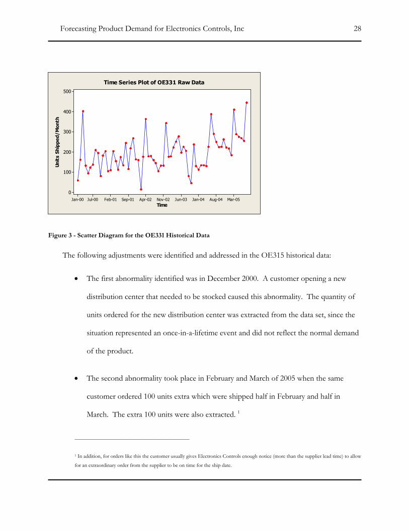
tools to identify any abnormalities in the data. Figures 1, 2 and 3 show the scatter diagrams of the
OE315, OE320 and OE331 historical data. Abnormalities are points that do not reflect the sales
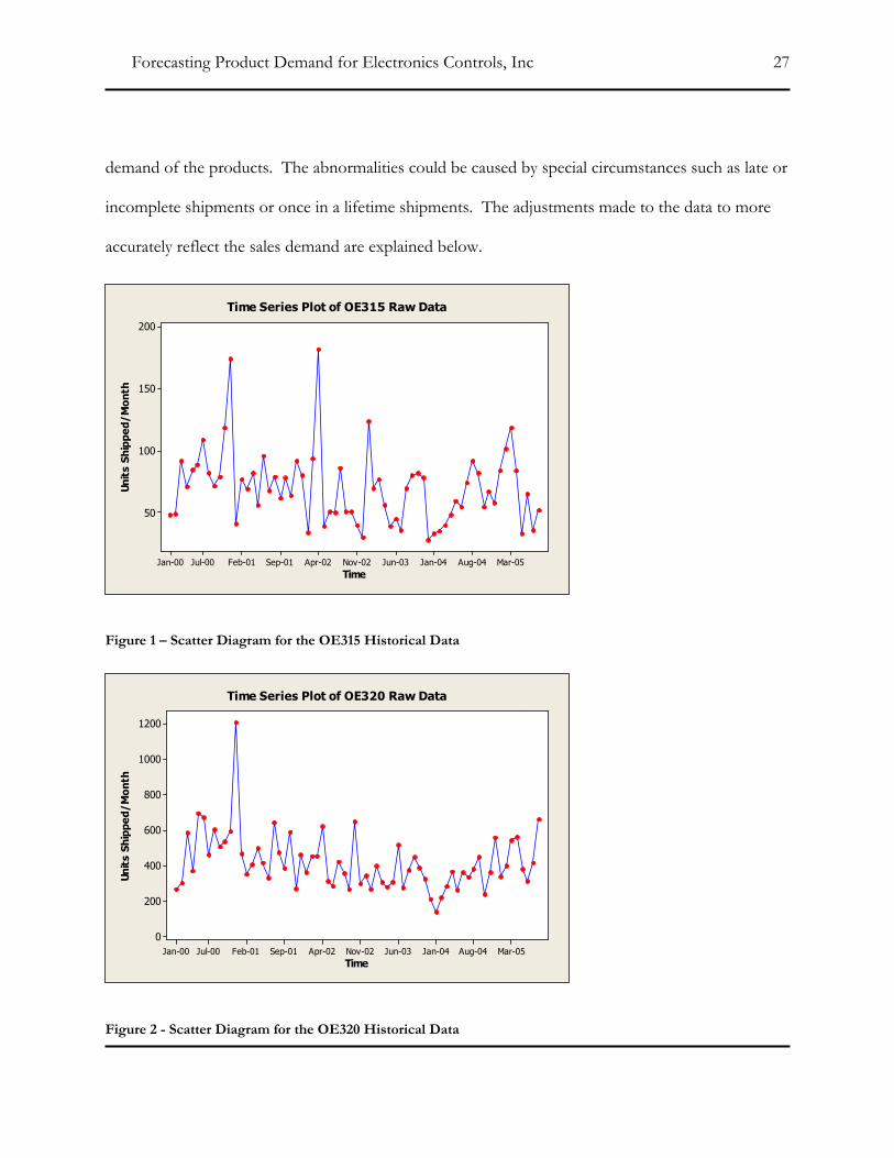
Forecasting Product Demand for Electronics Controls, Inc 27
demand of the products. The abnormalities could be caused by special circumstances such as late or
incomplete shipments or once in a lifetime shipments. The adjustments made to the data to more
accurately reflect the sales demand are explained below.
Time
Unit
s Sh
ippe
d/M
onth
Mar-05Aug-04Jan-04Jun-03Nov-02Apr-02Sep-01Feb-01Jul-00Jan-00
200
150
100
50
Time Series Plot of OE315 Raw Data
Figure 1 – Scatter Diagram for the OE315 Historical Data
Time
Unit
s Sh
ippe
d/M
onth
Mar-05Aug-04Jan-04Jun-03Nov-02Apr-02Sep-01Feb-01Jul-00Jan-00
1200
1000
800
600
400
200
0
Time Series Plot of OE320 Raw Data
Figure 2 - Scatter Diagram for the OE320 Historical Data
Forecasting Product Demand for Electronics Controls, Inc 28
Time
Unit
s Sh
ippe
d/M
onth
Mar-05Aug-04Jan-04Jun-03Nov-02Apr-02Sep-01Feb-01Jul-00Jan-00
500
400
300
200
100
0
Time Series Plot of OE331 Raw Data
Figure 3 - Scatter Diagram for the OE331 Historical Data
The following adjustments were identified and addressed in the OE315 historical data:
• The first abnormality identified was in December 2000. A customer opening a new
distribution center that needed to be stocked caused this abnormality. The quantity of
units ordered for the new distribution center was extracted from the data set, since the
situation represented an once-in-a-lifetime event and did not reflect the normal demand
of the product.
• The second abnormality took place in February and March of 2005 when the same
customer ordered 100 units extra which were shipped half in February and half in
March. The extra 100 units were also extracted. 1
_________________________________________________
1 In addition, for orders like this the customer usually gives Electronics Controls enough notice (more than the supplier lead time) to allow
for an extraordinary order from the supplier to be on time for the ship date.
Forecasting Product Demand for Electronics Controls, Inc 29
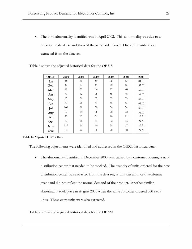
• The third abnormality identified was in April 2002. This abnormality was due to an
error in the database and showed the same order twice. One of the orders was
extracted from the data set.
Table 6 shows the adjusted historical data for the OE315.
OE315 2000 2001 2002 2003 2004 2005
Jan 48 41 80 124 33 84.00 Feb 49 77 34 70 35 52.00
Mar 92 69 94 77 40 69.00
Apr 71 82 96 56 48 84.00
May 85 56 39 39 59 33.00
Jun 89 96 51 45 55 65.00
Jul 109 68 50 36 74 36.00
Aug 82 79 86 70 92 52.00
Sep 72 62 51 80 82 N.A.
Oct 79 78 51 82 55 N.A.
Nov 119 64 40 78 67 N.A.
Dec 84 92 30 28 58 N.A.
Table 6- Adjusted OE315 Data
The following adjustments were identified and addressed in the OE320 historical data:
• The abnormality identified in December 2000; was caused by a customer opening a new
distribution center that needed to be stocked. The quantity of units ordered for the new
distribution center was extracted from the data set, as this was an once-in-a-lifetime
event and did not reflect the normal demand of the product. Another similar
abnormality took place in August 2005 when the same customer ordered 300 extra
units. These extra units were also extracted.
Table 7 shows the adjusted historical data for the OE320.

Forecasting Product Demand for Electronics Controls, Inc 30
OE320 2000 2001 2002 2003 2004 2005
Jan 265 467 360 265 136 337.00 Feb 302 354 451 399 222 397.00 Mar 583 406 453 305 283 543.00 Apr 369 497 620 279 364 560.00 May 694 415 310 308 262 378.00 Jun 669 330 286 515 360 309.00 Jul 463 645 419 275 335 417.00
Aug 603 477 355 374 380 363.00 Sep 509 385 265 448 447 N.A.
Oct 534 589 648 388 239 N.A.
Nov 592 270 299 326 361 N.A.
Dec 1208 462 344 211 559 N.A.
Table 7- Adjusted OE320 Data
The following adjustments were identified and addressed in the OE331 historical data:
• The abnormalities identified at points March 2000, December 2003, June 2004, March 2005 and August 2005 were caused by the introduction of new clients that needed a one-time solution to a specific problem. They needed a single or a couple of large orders and never ordered again. The orders from these customers were extracted since they did not reflect the normal demand of the product.
• The abnormality for April 2002 was due to Electronic Controls running out of inventory in February and sending double the amount of the product once the inventory recovered, which was in April. In this case, the double order was reduced by half for April and the other half was added to February.
Table 8 shows the adjusted historical data for the OE331.

Forecasting Product Demand for Electronics Controls, Inc 31
OE331 (Adjusted) 2000 2001 2002 2003 2004 2005
Jan 60 106 161 177 113 217.00 Feb 61 110 156 178 134 185.00 Mar 94 204 177 183 134 211.00 Apr 72 155 215 172 131 289.00 May 94 112 179 184 226 277.00 Jun 86 176 180 193 238 269.00 Jul 139 135 160 226 141 257.00
Aug 211 245 145 197 251 246.00 Sep 195 116 106 81 225 N.A.
Oct 81 219 133 47 227 N.A.
Nov 182 269 133 238 264 N.A.
Dec 205 165 344 131 224 N.A.
Table 8 - Adjusted OE331 Data
Model Building and Evaluation
The process of determining what method would best fit the 2000- 2004 data sets began after
the data were adjusted. The first step is to plot the products’ data sets to identify the components
present. The possible components are trend, seasonal, cyclical and irregular. Figures 4, 5 and 6
show the scatter diagram of the selected products’ adjusted historical data.

Forecasting Product Demand for Electronics Controls, Inc 32
Date
OE3
15 A
djus
ted
Dec-04Jun-04Dec-03Jun-03Dec-02Jun-02Dec-01Jun-01Dec-00Jun-00Jan-00
120
100
80
60
40
20
Time Series Plot of OE315 Adjusted
Figure 4 - Scatter Diagram for the OE315 Adjusted Data
Date
OE3
20 A
djus
ted
Dec-04Jun-04Dec-03Jun-03Dec-02Jun-02Dec-01Jun-01Dec-00Jun-00Jan-00
700
600
500
400
300
200
100
Time Series Plot of OE320 Adjusted
Figure 5 - Scatter Diagram for the OE320Adjusted Data

Forecasting Product Demand for Electronics Controls, Inc 33
Date
OE3
31 A
djus
ted
Dec-04Jun-04Dec-03Jun-03Dec-02Jun-02Dec-01Jun-01Dec-00Jun-00Jan-00
350
300
250
200
150
100
50
Time Series Plot of OE331 Adjusted
Figure 6 - Scatter Diagram for the OE331 Adjusted Data
The time series for both Figures 4 and 5 seem to have a slight trend downwards. In figure 4,
shipments decrease from about 80 to 60 units a month. In figure 5, shipments decrease from about
500 to 350 units a month. No other components (cyclical or seasonal) can be easily identified in
Figures 4 and 5. In Figure 6, the adjusted data seem to have a slight trend upward and no seasonal
or cyclical components appear to be present. The trend goes from about 100 to 200 units shipped
per month. Because the plots of the time series did not clearly show any seasonal or cyclical
components, the autocorrelation analysis for each of the time series was performed in an effort to
identify any overlooked components in the scatter diagram analysis.

Forecasting Product Demand for Electronics Controls, Inc 34
Lag
Aut
ocor
rela
tion
151413121110987654321
1.0
0.8
0.6
0.4
0.2
0.0
-0.2
-0.4
-0.6
-0.8
-1.0
Autocorrelation Function for OE315 Adjusted(with 5% significance limits for the autocorrelations)
Figure 7 - Autocorrelation Analysis for the OE315 Adjusted Data
Further analysis of the OE315 autocorrelation analysis (Figure 7) does not show signs of any
other component. A trend downward can be noticed in the first three lags. For the OE315 the Q
statistic for 15 lags is 12.14, less than the Chi-square value of 24.99 tested at the 5% significance
level. Thus, statistically, it appears that the series is random.

Forecasting Product Demand for Electronics Controls, Inc 35
Lag
Aut
ocor
rela
tion
151413121110987654321
1.0
0.8
0.6
0.4
0.2
0.0
-0.2
-0.4
-0.6
-0.8
-1.0
Autocorrelation Function for OE320 Adjusted(with 5% significance limits for the autocorrelations)
Figure 8 - Autocorrelation Analysis for the OE320 Adjusted Data
The autocorrelation analysis of the OE320 (Figure 8) displays somewhat of a trend in the first
three lags and a possible cyclical component every three lags. For the OE320 the Q statistic for 15
lags is 31.83, greater than the Chi-square value of 24.99 tested at the 5% significance level. Thus,
statistically, it appears that the series is not random.
Forecasting Product Demand for Electronics Controls, Inc 36
Lag
Aut
ocor
rela
tion
151413121110987654321
1.0
0.8
0.6
0.4
0.2
0.0
-0.2
-0.4
-0.6
-0.8
-1.0
Autocorrelation Function for OE331(Adjusted)(with 5% significance limits for the autocorrelations)
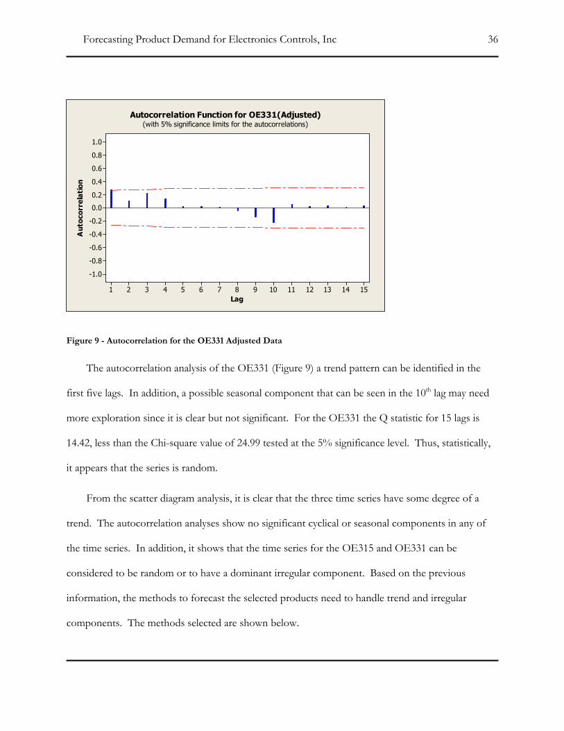
Figure 9 - Autocorrelation for the OE331 Adjusted Data
The autocorrelation analysis of the OE331 (Figure 9) a trend pattern can be identified in the
first five lags. In addition, a possible seasonal component that can be seen in the 10th lag may need
more exploration since it is clear but not significant. For the OE331 the Q statistic for 15 lags is
14.42, less than the Chi-square value of 24.99 tested at the 5% significance level. Thus, statistically,
it appears that the series is random.
From the scatter diagram analysis, it is clear that the three time series have some degree of a
trend. The autocorrelation analyses show no significant cyclical or seasonal components in any of
the time series. In addition, it shows that the time series for the OE315 and OE331 can be
considered to be random or to have a dominant irregular component. Based on the previous
information, the methods to forecast the selected products need to handle trend and irregular
components. The methods selected are shown below.

Forecasting Product Demand for Electronics Controls, Inc 37
• Naïve effectively handles irregular component.
• Linear Regression effectively handles trend component.
• Moving Average effectively handles irregular component.
• Simple Exponential effectively handles irregular component.
• Double exponential effectively handles irregular and trend components.
Table 9, Table 10 and Table 11 summarize the methods used in this section, the parameters that
were selected to do the forecast and the accuracy measures for the three selected products.
OE315
Naive Linear Regression Moving Averaging Exponential Double Exponential
Yt = 123.744 + 1.35049*t
k = 11 Alpha = 0.08155
Alpha (level) 0.695 Beta (trend) 0.044
MAPE 33.473 MAD 20.712 MSD 764.542
MAPE 31.123 MAD 17.404 MSD 444.580
MAPE 32.616 MAD 18.06 MSD 503.063
MAPE 33.153 MAD 17.849 MSD 483.028
MAPE 31.543 MAD 18.951 MSD 652.197
Table 9- Results from Model-Base Forecasting Methods for the OE315
For the OE315, the forecast created following the linear regression method produced the
smallest MSD followed by the MSD from the simple exponential method. The values for the MAD
of all the different forecasting method were similar to each other, producing a range from the
smallest to the largest of only three units. The same observation was true for the values MAPE
values, since the range of variation was only 2% between all the different methods. Because of the
previous information, the linear regression and the simple exponential method are the most accurate
for the OE315.
Forecasting Product Demand for Electronics Controls, Inc 38
OE320
Naive Linear Regression Moving Averaging Exponential Double Exponential
Yt = 504.176 - 3.31562*t
k = 6 Alpha 0.134377 Alpha (level) 0.417 Beta (trend) 0.0544
MAPE 32.9 MAD 125.8 MSD 24463.1
MAPE 25.8 MAD 92.2 MSD 12885.8
MAPE 26.0 MAD 89.7 MSD 12375.7
MAPE 27.5 MAD 96.8 MSD 14119.4
MAPE 26.4 MAD 99.9 MSD 15773.2
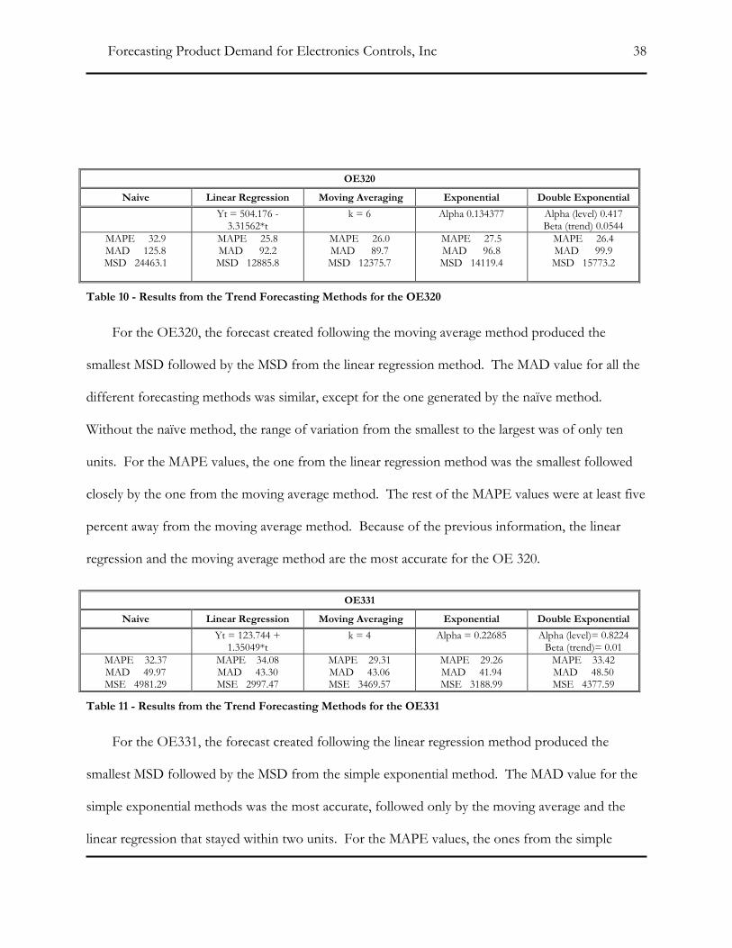
Table 10 - Results from the Trend Forecasting Methods for the OE320
For the OE320, the forecast created following the moving average method produced the
smallest MSD followed by the MSD from the linear regression method. The MAD value for all the
different forecasting methods was similar, except for the one generated by the naïve method.
Without the naïve method, the range of variation from the smallest to the largest was of only ten
units. For the MAPE values, the one from the linear regression method was the smallest followed
closely by the one from the moving average method. The rest of the MAPE values were at least five
percent away from the moving average method. Because of the previous information, the linear
regression and the moving average method are the most accurate for the OE 320.
OE331
Naive Linear Regression Moving Averaging Exponential Double Exponential
Yt = 123.744 + 1.35049*t
k = 4 Alpha = 0.22685 Alpha (level)= 0.8224 Beta (trend)= 0.01
MAPE 32.37 MAD 49.97 MSE 4981.29
MAPE 34.08 MAD 43.30 MSE 2997.47
MAPE 29.31 MAD 43.06 MSE 3469.57
MAPE 29.26 MAD 41.94 MSE 3188.99
MAPE 33.42 MAD 48.50 MSE 4377.59
Table 11 - Results from the Trend Forecasting Methods for the OE331
For the OE331, the forecast created following the linear regression method produced the
smallest MSD followed by the MSD from the simple exponential method. The MAD value for the
simple exponential methods was the most accurate, followed only by the moving average and the
linear regression that stayed within two units. For the MAPE values, the ones from the simple
Forecasting Product Demand for Electronics Controls, Inc 39
exponential method were the smallest followed closely by the ones from the moving average
method. The rest of the MAPE values were at most five percent away from the moving average
method. Because of the previous information, the linear regression and the simple exponential
method are the most accurate for the OE 331.
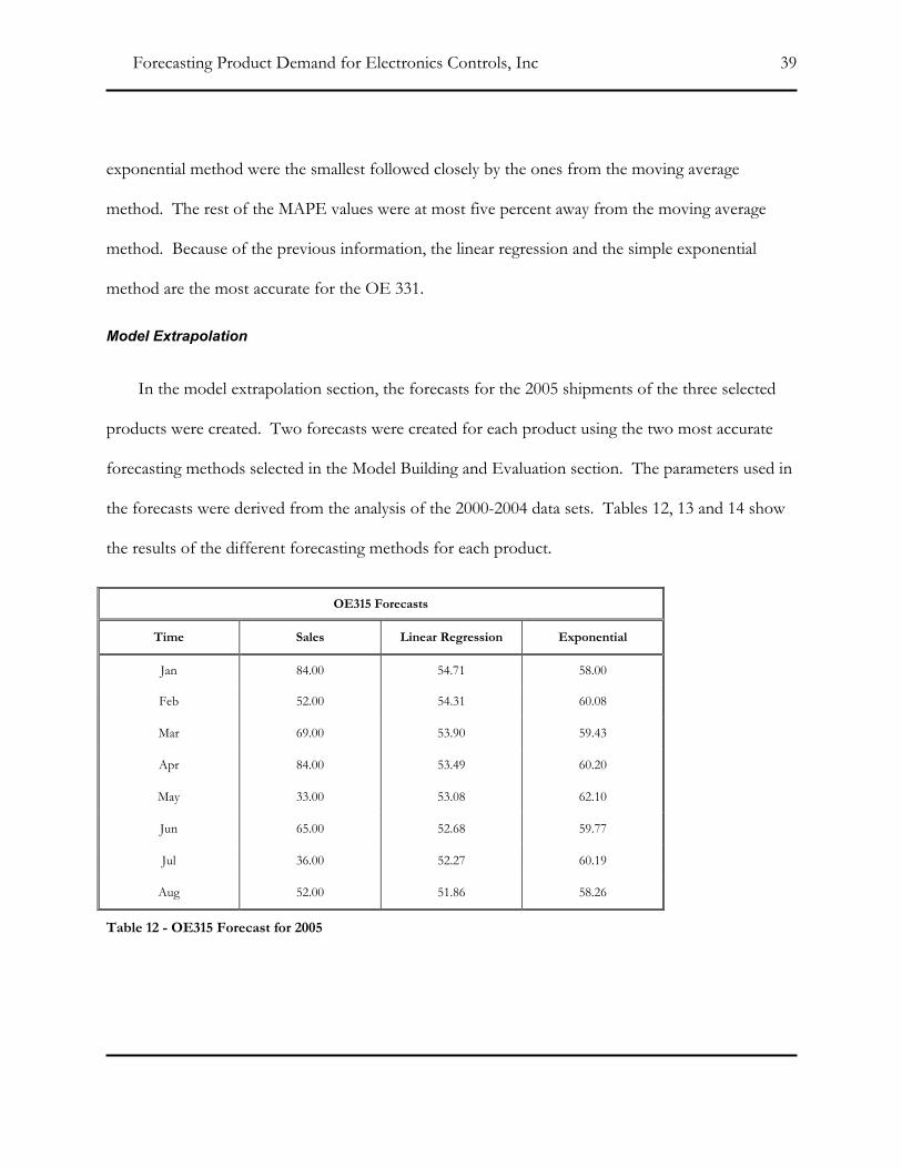
Model Extrapolation
In the model extrapolation section, the forecasts for the 2005 shipments of the three selected
products were created. Two forecasts were created for each product using the two most accurate
forecasting methods selected in the Model Building and Evaluation section. The parameters used in
the forecasts were derived from the analysis of the 2000-2004 data sets. Tables 12, 13 and 14 show
the results of the different forecasting methods for each product.
OE315 Forecasts
Time Sales Linear Regression Exponential
Jan 84.00 54.71 58.00
Feb 52.00 54.31 60.08
Mar 69.00 53.90 59.43
Apr 84.00 53.49 60.20
May 33.00 53.08 62.10
Jun 65.00 52.68 59.77
Jul 36.00 52.27 60.19
Aug 52.00 51.86 58.26
Table 12 - OE315 Forecast for 2005

Forecasting Product Demand for Electronics Controls, Inc 40
OE320 Forecasts
Time Sales Moving Average Linear Regression
Jan 337.00 386.83 301.92
Feb 397.00 387.17 298.61
Mar 543.00 390.00 295.29
Apr 560.00 406.00 291.98
May 378.00 459.50 288.66
Jun 309.00 462.33 285.35
Jul 417.00 420.67 282.03
Aug 363.00 434.00 278.71
Table 13 - OE320 Forecast for 2005
OE331 Forecasts
Time Sales Exponential Linear Regression
Jan 217.00 228.00 206.12
Feb 185.00 227.12 207.47
Mar 211.00 223.75 208.82
Apr 289.00 238.73 210.18
May 277.00 242.75 211.53
Jun 269.00 245.49 212.88
Jul 257.00 247.37 214.23
Aug 246.00 248.14 215.58
Table 14 - OE331 Forecast for 2005
Forecasting Product Demand for Electronics Controls, Inc 41
Forecast Evaluation
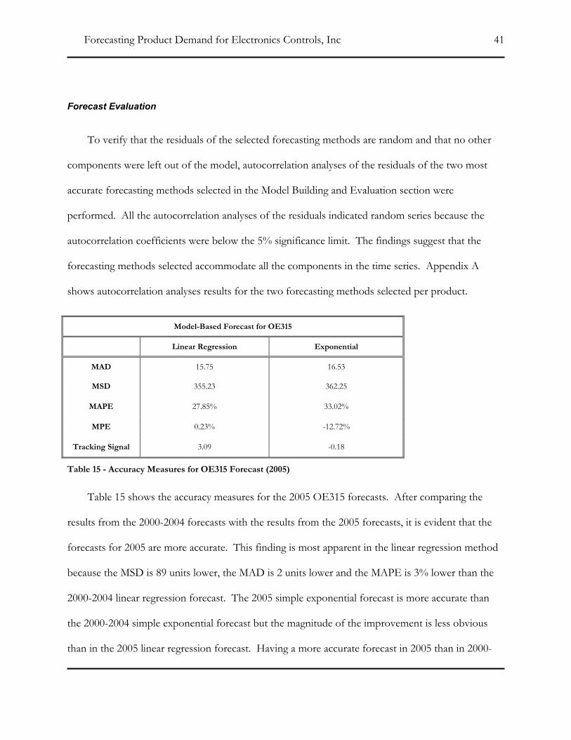
To verify that the residuals of the selected forecasting methods are random and that no other
components were left out of the model, autocorrelation analyses of the residuals of the two most
accurate forecasting methods selected in the Model Building and Evaluation section were
performed. All the autocorrelation analyses of the residuals indicated random series because the
autocorrelation coefficients were below the 5% significance limit. The findings suggest that the
forecasting methods selected accommodate all the components in the time series. Appendix A
shows autocorrelation analyses results for the two forecasting methods selected per product.
Model-Based Forecast for OE315
Linear Regression Exponential
MAD 15.75 16.53
MSD 355.23 362.25
MAPE 27.85% 33.02%
MPE 0.23% -12.72%
Tracking Signal 3.09 -0.18
Table 15 - Accuracy Measures for OE315 Forecast (2005)
Table 15 shows the accuracy measures for the 2005 OE315 forecasts. After comparing the
results from the 2000-2004 forecasts with the results from the 2005 forecasts, it is evident that the
forecasts for 2005 are more accurate. This finding is most apparent in the linear regression method
because the MSD is 89 units lower, the MAD is 2 units lower and the MAPE is 3% lower than the
2000-2004 linear regression forecast. The 2005 simple exponential forecast is more accurate than
the 2000-2004 simple exponential forecast but the magnitude of the improvement is less obvious
than in the 2005 linear regression forecast. Having a more accurate forecast in 2005 than in 2000-

Forecasting Product Demand for Electronics Controls, Inc 42
2004 indicates that the parameters selected for the linear regression and the simple exponential
methods continue to be appropriate in 2005. In addition, both tracking signals are below ±5 (linear
regression 3.09, simple exponential -0.18), which reiterates that the parameters continue to be
appropriate in 2005.
Model-Based Forecast for OE320
Moving Average Linear Regression
MAD 84.52 122.68
MSD 10614.11 22246.11
MAPE 20.57% 26.94%
MPE -6.03% 26.94%
Tracking Signal -0.50 8.0
Table 16 - Accuracy Measures for OE320 Forecast (2005)
Table 16 shows the accuracy measures for the 2005 OE320 forecasts. After comparing the
results from the 2000-2004 moving average forecast with the results from the 2005 moving average
forecast, it is evident that the 2005 results are more accurate. The MAD is 5.6 units lower, the MSD
is 2271 units lower and the MAPE is 5.4% lower than the 2000-2004 moving average forecast.
Having a more accurate forecast in 2005 than in 2000-2004 indicates that the parameters selected for
the moving average method continue to be appropriate in 2005. In addition, the tracking signal is
well below ±5 (-0.5), which reiterates that the parameters continue to be appropriate in 2005.
Comparing the results from the 2000-2004 linear regression forecast with the results from the
2005 linear regression forecast shows that the 2005 results are less accurate. The MAD is 30.5 units
higher, the MSD is 9360 units higher and the MAPE is 0.3% higher than the 2000-2004 linear
regression forecast. Having a less accurate forecast in 2005 than in 2000-2004 indicates that the
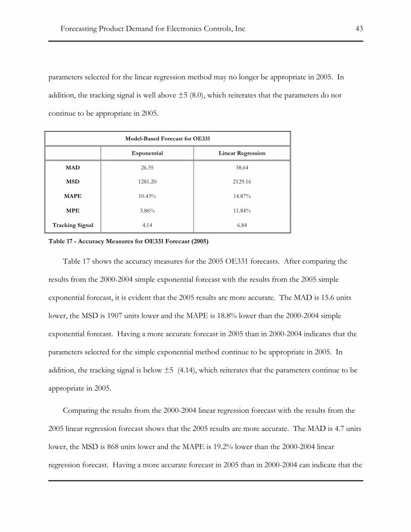
Forecasting Product Demand for Electronics Controls, Inc 43
parameters selected for the linear regression method may no longer be appropriate in 2005. In
addition, the tracking signal is well above ±5 (8.0), which reiterates that the parameters do not
continue to be appropriate in 2005.
Model-Based Forecast for OE331
Exponential Linear Regression
MAD 26.35 38.64
MSD 1281.20 2129.16
MAPE 10.43% 14.87%
MPE 3.86% 11.84%
Tracking Signal 4.14 6.84
Table 17 - Accuracy Measures for OE331 Forecast (2005)
Table 17 shows the accuracy measures for the 2005 OE331 forecasts. After comparing the
results from the 2000-2004 simple exponential forecast with the results from the 2005 simple
exponential forecast, it is evident that the 2005 results are more accurate. The MAD is 15.6 units
lower, the MSD is 1907 units lower and the MAPE is 18.8% lower than the 2000-2004 simple
exponential forecast. Having a more accurate forecast in 2005 than in 2000-2004 indicates that the
parameters selected for the simple exponential method continue to be appropriate in 2005. In
addition, the tracking signal is below ±5 (4.14), which reiterates that the parameters continue to be
appropriate in 2005.
Comparing the results from the 2000-2004 linear regression forecast with the results from the
2005 linear regression forecast shows that the 2005 results are more accurate. The MAD is 4.7 units
lower, the MSD is 868 units lower and the MAPE is 19.2% lower than the 2000-2004 linear
regression forecast. Having a more accurate forecast in 2005 than in 2000-2004 can indicate that the

Forecasting Product Demand for Electronics Controls, Inc 44
parameters selected for the linear regression method continue to be appropriate in 2005. On the
other hand, the tracking signal is well above ±5 (6.8), which means that the parameters might not
be appropriate in 2005. While the accuracy parameters remained stable, the tracking signal indicates
that the linear regression method is constantly underestimating the real values, giving a strong
indication that the parameter are no longer accurate.
Of all the forecasting methods analyzed in this section, the only ones that fail to prove that their
parameters continue to be appropriate are the linear regressions for the OE320 and OE331. The
main cause of the linear regression failure is suspected to be the range of the fitting data set (2000-
2004). Older data may not be relevant to calculate future value forecasts. To see if using data that
are more recent improves the results, new forecasts were created using only the previous 12 months
up to the point to be forecasted as the fitting data set.
OE 320 12 months Linear Regression
Month Sales Forecast Equation Accuracy Measures
Jan 337.00 473.09 y = 22.168x + 184.91 MAD = 101.64
Feb 397.00 434.82 y = 13.703x + 256.68 MSD = 12830.99
Mar 543.00 425.66 y = 10.049x + 295.02 MAPE = 26.58%
Apr 560.00 470.13 y = 13.559x + 293.86 MPE = -17.16%
May 378.00 525.65 y = 19.587x + 271.02 Tracking Signal = -3.92
Jun 309.00 489.95 y = 12.608x + 326.05
Jul 417.00 446.78 y = 6.6189x + 360.73
Aug 363.00 436.61 y = 4.0035x + 384.56
Table 18 - Forecast and Accuracy Measures for the OE320 12 Month Linear Regression
Table 18 shows the results of the adjustments in the OE320 linear regression method for 2005.
The new accuracy measures are an improvement over the original 2005 forecast: The MAD

Forecasting Product Demand for Electronics Controls, Inc 45
decreased by 21.0 units and the MSD decreased by 9415 units. The most significant result is the
reduction of the tracking signal to the acceptable level of 3.92. Therefore, the adjusted forecast
(seen in Table 18) replaces the original linear regression method (seen in Table 13) for the remainder
of the project.
OE 331 12 months Linear Regression
Month Sales Forecast Equation Accuracy Measures
Jan 217.00 271.66 y = 12.203x + 113.02 MAD =38.02
Feb 185.00 263.04 y = 9.5455x + 138.95 MSD = 1953.00
Mar 211.00 243.50 y = 5.8846x + 167 MAPE = 16.66%
Apr 289.00 230.30 y = 2.8671x + 193.03 MPE = -7.00%
May 277.00 238.97 y = 2.1748x + 210.7 Signal Tracking =-2.26
Jun 269.00 256.61 y = 4.2343x + 201.56
Jul 257.00 271.80 y = 6.1748x + 191.53
Aug 246.00 261.01 y = 3.028x + 221.65
Table 19 - Forecast and Accuracy Measures for the OE331 12 Months Linear Regression
Table 19 shows the results of the adjustments in the OE331 linear regression method for 2005.
The new accuracy measures are very similar to the original 2005 forecast: The MAD decreased by
0.60 units, the MSD decreased by 176 units and the MAPE decreased by 2%. The most significant
change is the reduction of the tracking signal to the acceptable level of 2.26. Having the tracking
signal at an acceptable level warrants using the adjusted forecast (seen in Table 19) to replace the
original linear regression method (seen in Table 14) for the remainder of the project.
Once the forecasts have acceptable parameters, one forecasting method is selected for each
product based on the accuracy measures. The most accurate method for the OE315 is the linear
regression method, for the OE320 it is the moving average method and for the OE331 it is the
Forecasting Product Demand for Electronics Controls, Inc 46
simple exponential method. The forecasts from these methods are considered the end-result of the
entire model-based process. In the next section, the results from the model-based process are
compared to the forecasts that the current Electronic Controls’ process developed for 2005.
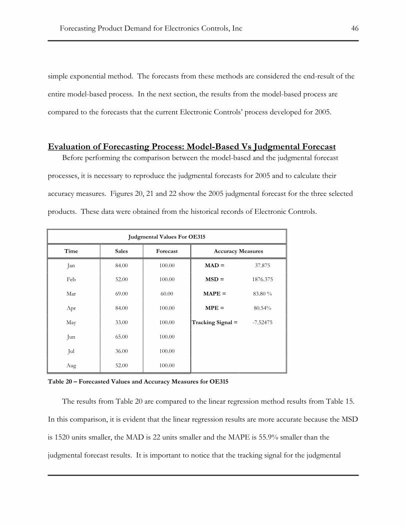
Evaluation of Forecasting Process: Model-Based Vs Judgmental Forecast Before performing the comparison between the model-based and the judgmental forecast
processes, it is necessary to reproduce the judgmental forecasts for 2005 and to calculate their
accuracy measures. Figures 20, 21 and 22 show the 2005 judgmental forecast for the three selected
products. These data were obtained from the historical records of Electronic Controls.
Judgmental Values For OE315
Time Sales Forecast Accuracy Measures
Jan 84.00 100.00 MAD = 37.875
Feb 52.00 100.00 MSD = 1876.375
Mar 69.00 60.00 MAPE = 83.80 %
Apr 84.00 100.00 MPE = 80.54%
May 33.00 100.00 Tracking Signal = -7.52475
Jun 65.00 100.00
Jul 36.00 100.00
Aug 52.00 100.00
Table 20 – Forecasted Values and Accuracy Measures for OE315
The results from Table 20 are compared to the linear regression method results from Table 15.
In this comparison, it is evident that the linear regression results are more accurate because the MSD
is 1520 units smaller, the MAD is 22 units smaller and the MAPE is 55.9% smaller than the
judgmental forecast results. It is important to notice that the tracking signal for the judgmental
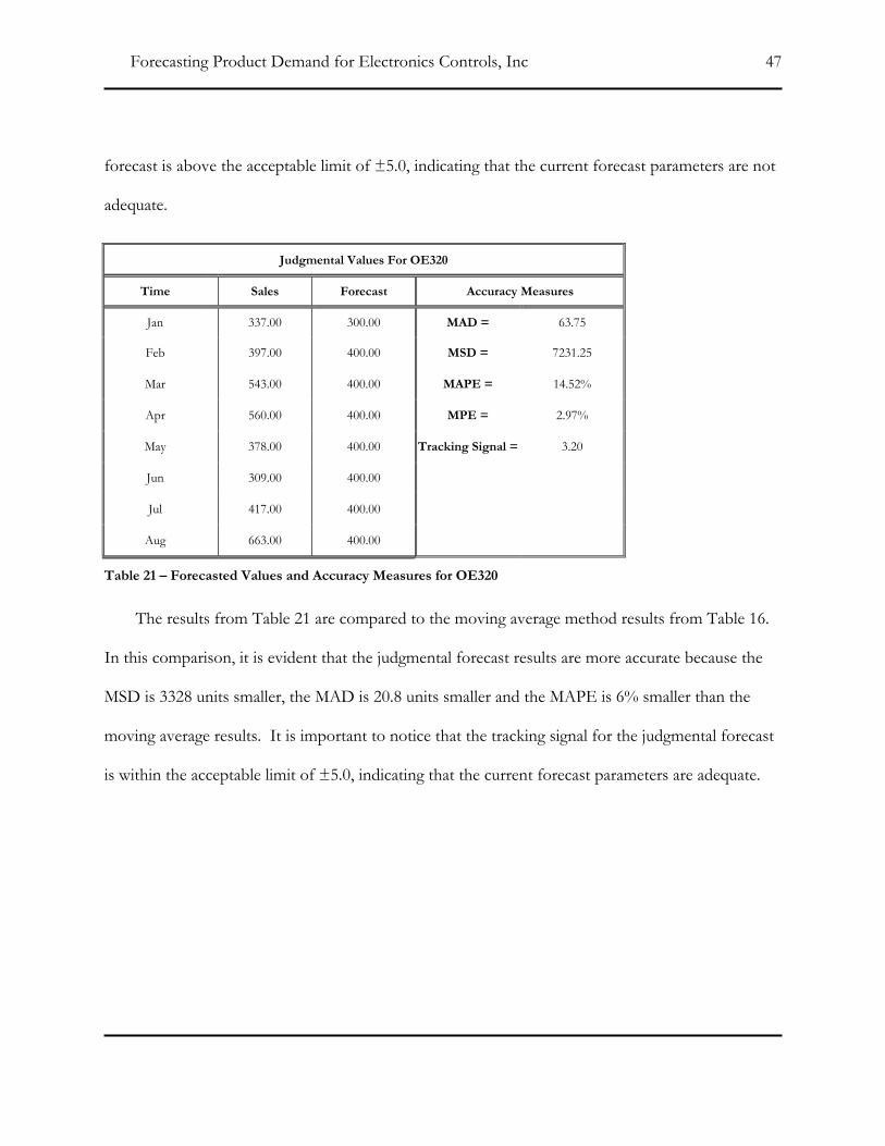
Forecasting Product Demand for Electronics Controls, Inc 47
forecast is above the acceptable limit of ±5.0, indicating that the current forecast parameters are not
adequate.
Judgmental Values For OE320
Time Sales Forecast Accuracy Measures
Jan 337.00 300.00 MAD = 63.75
Feb 397.00 400.00 MSD = 7231.25
Mar 543.00 400.00 MAPE = 14.52%
Apr 560.00 400.00 MPE = 2.97%
May 378.00 400.00 Tracking Signal = 3.20
Jun 309.00 400.00
Jul 417.00 400.00
Aug 663.00 400.00
Table 21 – Forecasted Values and Accuracy Measures for OE320
The results from Table 21 are compared to the moving average method results from Table 16.
In this comparison, it is evident that the judgmental forecast results are more accurate because the
MSD is 3328 units smaller, the MAD is 20.8 units smaller and the MAPE is 6% smaller than the
moving average results. It is important to notice that the tracking signal for the judgmental forecast
is within the acceptable limit of ±5.0, indicating that the current forecast parameters are adequate.

Forecasting Product Demand for Electronics Controls, Inc 48
Judgmental Values For OE331
Time Sales Forecast Accuracy Measures
Jan 217.00 200.00 MAD = 35.375
Feb 185.00 200.00 MSD = 1851.375
Mar 211.00 300.00 MAPE = 15.10%
Apr 289.00 300.00 MPE = 13.10%
May 277.00 300.00 Tracking Signal = -7.04
Jun 269.00 300.00
Jul 257.00 300.00
Aug 246.00 300.00
Table 22– Forecasted Values and Accuracy Measures for OE331
The results from Table 22 are compared to the simple exponential method results from Table
17. In this comparison, it is evident that the simple exponential results are more accurate because
the MSD is 570 units smaller, the MAD is 9 units smaller and the MAPE is 4.7% smaller than the
judgmental forecast results. It is important to notice that the tracking signal for the judgmental
forecast is above the acceptable limit of ±5.0, indicating that the current forecast parameters are not
adequate.

Forecasting Product Demand for Electronics Controls, Inc 49
Conclusions and Recommendations
The following are the main conclusions from the analyses generated during this project:
1. The study of the current Electronic Controls, Inc. forecasting process shows that the
process is highly dependant on the knowledge and instincts of the experts that produce the
forecast. Even when historical data are analyzed, the resulting forecast can be considered a
judgmental one.
2. During the creation of a model-based process for the selected products the following was
encountered:
2.1. Ideally, sales data should be utilized when forecasting the demand of a product.
Electronic Controls does not keep record of this data, therefore shipping data were used
instead. Shipping data are not optimal in the creation of a forecast for the demand of a
product because shipments can be delayed or only partially shipped. In order to use
shipping data, the abnormalities must be filtered out in order for the shipping data to
reflect sales demand more accurately.
2.2. The 2000-20004 data sets had a dominant irregular component that made the OE315
and OE331 appear to be random.
2.3. The most accurate forecasting methods for each product are different. For the OE315
it is the linear regression, for the OE320 it is the moving average and, for the OE331, it
is the single exponential.

Forecasting Product Demand for Electronics Controls, Inc 50
2.4. Using the 2000-2004 data sets to calculate the parameters for each forecasting method is
not optimal for all methods. Calculating the linear regression parameters using the
previous 12 months up to the forecasting point gives better results for the OE320 and
the OE331.
3. When the accuracy measures were calculated for the current judgmental based forecasting
process, it was observed that the forecasts for the OE315 and the OE331 were inaccurate.
Their tracking signals fell outside of the acceptable range, indicating that the current
forecasting parameters were not appropriate.
4. When comparing the model-based process to the judgmental based process, the model-
based forecasts gave results that are more accurate for the OE315 and the OE331. The
judgmental-based forecasts gave better results only for the OE320.
After analyzing information gathered in this project, it is recommended that Electronic
Controls implement some or all of the following suggestions to improve their current forecasting
process.
1. Electronic Controls needs to keep records of the quantities of products sold per month.
The sales data can be used instead of the shipping data to produce forecasts that are more
accurate.
2. Electronic Controls needs to keep track of the forecasting error in order to maintain updated
accuracy measures. Having updated accuracy measures would give the experts a better
indication of how the forecast is performing allowing them to adjust more quickly thus
making the forecasts more accurate.

Forecasting Product Demand for Electronics Controls, Inc 51
3. The current judgmental process could be fine tuned by using a tracking signal to produce a
more accurate forecast. The tracking signal could eliminate inaccurate parameters such as
the ones observed in the OE315 and OE331 forecasts.
4. The model-based methods can be applied as a tool to make a complete and informed
judgment of future product demand.
5. Electronic Controls uses only tabular format to analyze the data utilized to generate the
demand forecast as is shown in Table 1 and Table 2. Changing the data to a graphical
format may benefit the accuracy of the forecast because it would allow the experts to
visualize the fluctuations of the historical data (Clements, 2002).

Forecasting Product Demand for Electronics Controls, Inc 52
Suggestions for Additional Work
Several questions that fell outside of the scope of this project were raised during its
development. In order to gain a full understanding of the needs of inventory control forecasting,
further research can be performed with respect to those questions. The following is a list of some
of the questions and topics to be researched in the future:
1. Finding the most accurate method for each product might be too time consuming when
trying to forecast the demand of the entire range of products offered by Electronic Controls.
Further studies need to be performed with the goal of finding one or few method(s) that are
most effective in handling Electronic Controls’ full range of products. A variation could be
to study how to categorize the products in the hopes of limiting the number of forecasting
methods to one per category. Products could be categorized as follows: Products with high,
medium and low sales volumes or products at different stages of their lifecycles.
2. The fitting period from 2000-2004 was not optimal for all the forecasting methods. More
investigation is needed to find the optimal fitting period for the different forecasting
methods and to find how to identify which historical data are relevant and which are not.
3. This project was based on monthly demand for three products. Some products might give
forecasts that are more accurate when a different time period is selected. For some products
it is harder to change the amount of units delivered as opposed to changing the delivery date.
Some studies can be performed to see if changing the delivery date instead of the amount of
units delivered could produce similar or better accuracy measures.

Forecasting Product Demand for Electronics Controls, Inc 53
4. Further research can be performed on calculating safety stocks, reordering levels and lot size
from the forecast results. The final goal of having an accurate forecast is to be able to
maintain more efficient inventory levels.
5. Most of the accounting and inventory control software packages have forecasting modules.
It may be in the best interest of the company to investigate what the state of the art is in
forecasting software modules.

Forecasting Product Demand for Electronics Controls, Inc 54
References / Bibliography
Axsäter, Sven. 2000. Inventory Control. Boston: Kluwer Academic Publishers.
Bowerman, Bruce L., Richard T. O’Connell and Anne B. Koehler. 2005. Forecasting, Time Series, and
Regression. Fourth Edition. Belmont: Thomson Brooks/Cole.
Clements, Michael P., and David F. Hendry, eds. 2002. A Compantion to Economic Forecasting.
Massachusetts: Blackwell Publishers Inc.
De Kok, A.G. 1987. Product Inventory Control Models: Approximations and Algorithms. Amsterdam: CWI
Tracts.
Hanke, John E. Dean W. Wichern and Arthur G. Reitsch. 2001. Business Forecasting. Seventh
Edition. Upper Saddle River: Prentice Hall.
Harris, Richard and Robert Sollis. 2003. Applied Time Series Modelling and Forecasting. Chichester:
John Wiley & Sons Ltd.
Knight, John and Stephen Satchell, eds. 2002. Forecasting Volatility in the Financial Markets. Second
Edition. Woburn: Elsevier Science Ltd.
MINITAB [Computer Software]. 2005. State College. PA: Minitab, Inc.
Seth, Suresh P., Houmin Yan and Hanqin Zhang. 2005. Inventory and Supply Chain Management with
Forecast Updates. New York: Springer Science+Business Media, Inc.

Forecasting Product Demand for Electronics Controls, Inc 55
Toomey, John W. 2000. Inventory Management: Principles, Concepts and Techniques. Boston: Kluwer
Academic Publishers.
Zellner, Arnold. 2004. Statistics, Econometrics and Forecasting. Cambridge: Cambridge University Press.

Forecasting Product Demand for Electronics Controls, Inc 56
APPENDIX A

Forecasting Product Demand for Electronics Controls, Inc 57
Lag
Aut
ocor
rela
tion
151413121110987654321
1.0
0.8
0.6
0.4
0.2
0.0
-0.2
-0.4
-0.6
-0.8
-1.0
Autocorrelation Function for OE315 Linear Regression Residuals(with 5% significance limits for the autocorrelations)
Figure 10 – Autocorrelation Function for the OE315 Linear Regression
Lag
Aut
ocor
rela
tion
151413121110987654321
1.0
0.8
0.6
0.4
0.2
0.0
-0.2
-0.4
-0.6
-0.8
-1.0
Autocorrelation Function for OE315 Exponential Residuals(with 5% significance limits for the autocorrelations)
Figure 11– Autocorrelation Function for the OE315 Exponential

Forecasting Product Demand for Electronics Controls, Inc 58
Lag
Aut
ocor
rela
tion
151413121110987654321
1.0
0.8
0.6
0.4
0.2
0.0
-0.2
-0.4
-0.6
-0.8
-1.0
Autocorrelation Function for OE320 Linear Regression Residuals(with 5% significance limits for the autocorrelations)
Figure 12– Autocorrelation Function for the OE320 Linear Regression
Lag
Aut
ocor
rela
tion
1413121110987654321
1.0
0.8
0.6
0.4
0.2
0.0
-0.2
-0.4
-0.6
-0.8
-1.0
Autocorrelation Function for OE320 Moving Average Residuals(with 5% significance limits for the autocorrelations)
Figure 13– Autocorrelation Function for the OE320 Moving Average

Forecasting Product Demand for Electronics Controls, Inc
59
Lag
Aut
ocor
rela
tion
151413121110987654321
1.0
0.8
0.6
0.4
0.2
0.0
-0.2
-0.4
-0.6
-0.8
-1.0
Autocorrelation Function for OE331 Linear Regression Residuals(with 5% significance limits for the autocorrelations)
Figure 14– Autocorrelation Function for the OE331 Linear Regression
Lag
Aut
ocor
rela
tion
151413121110987654321
1.0
0.8
0.6
0.4
0.2
0.0
-0.2
-0.4
-0.6
-0.8
-1.0
Autocorrelation Function for OE331 Exponetial Residuals(with 5% significance limits for the autocorrelations)
Figure 15– Autocorrelation Function for the OE331 Exponential