Lecture 9: Variance, Covariance, Correlation -
76
beamer-tu-log Variance Covariance Correlation coefficient Lecture 9: Variance, Covariance, Correlation Coefficient Kateˇ rina Sta ˇ nková Statistics (MAT1003) May 2, 2012
Transcript of Lecture 9: Variance, Covariance, Correlation -
beamer-tu-logo
Variance Covariance Correlation coefficient
Lecture 9: Variance, Covariance,Correlation Coefficient
Katerina Stanková
Statistics (MAT1003)
May 2, 2012
beamer-tu-logo
Variance Covariance Correlation coefficient
Outline
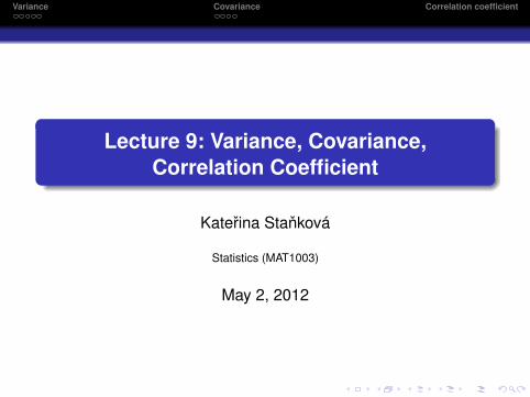
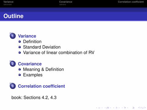
1 VarianceDefinitionStandard DeviationVariance of linear combination of RV
2 CovarianceMeaning & DefinitionExamples
3 Correlation coefficient
book: Sections 4.2, 4.3
beamer-tu-logo
Variance Covariance Correlation coefficient
And now . . .
1 VarianceDefinitionStandard DeviationVariance of linear combination of RV
2 CovarianceMeaning & DefinitionExamples
3 Correlation coefficient
beamer-tu-logo
Variance Covariance Correlation coefficient
Definition
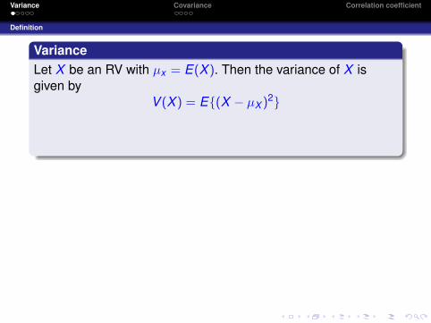
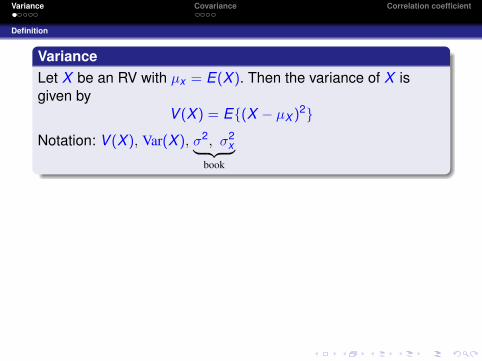
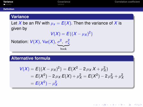
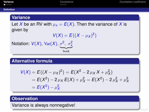
VarianceLet X be an RV with µx = E(X ). Then the variance of X isgiven by
V (X ) = E{(X − µX )2}
Notation: V (X ), Var(X ), σ2, σ2x︸ ︷︷ ︸
book
Alternative formula
V (X ) = E{(X − µX )2} = E(X 2 − 2µX X + µ2
X )
= E(X 2)− 2µX E(X ) + µ2X = E(X 2)− 2µ2
X + µ2X
= E(X 2)− µ2X
ObservationVariance is always nonnegative!
beamer-tu-logo
Variance Covariance Correlation coefficient
Definition
VarianceLet X be an RV with µx = E(X ). Then the variance of X isgiven by
V (X ) = E{(X − µX )2}
Notation: V (X ), Var(X ), σ2, σ2x︸ ︷︷ ︸
book
Alternative formula
V (X ) = E{(X − µX )2} = E(X 2 − 2µX X + µ2
X )
= E(X 2)− 2µX E(X ) + µ2X = E(X 2)− 2µ2
X + µ2X
= E(X 2)− µ2X
ObservationVariance is always nonnegative!
beamer-tu-logo
Variance Covariance Correlation coefficient
Standard Deviation
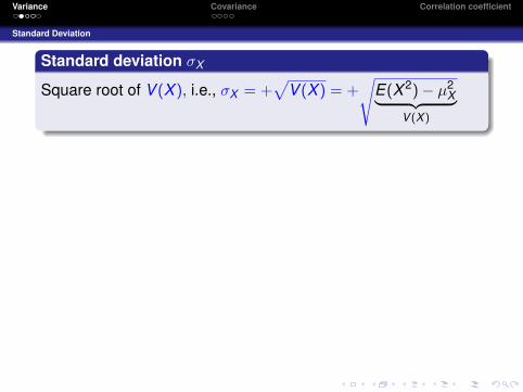
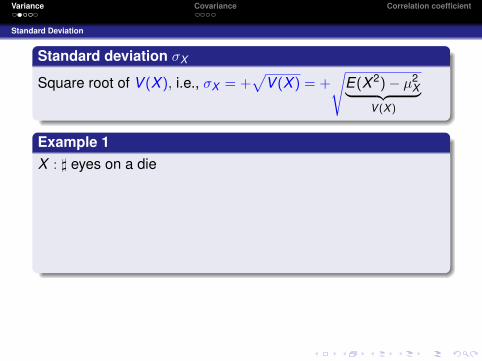
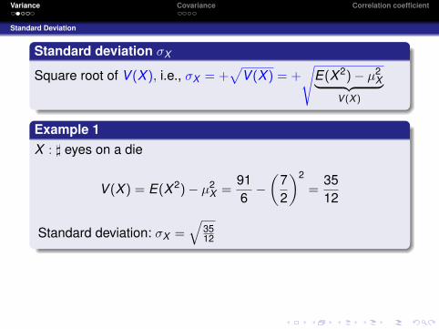
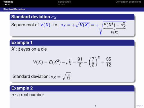
Standard deviation σX
Square root of V (X ), i.e., σX = +√
V (X ) = +√
E(X 2)− µ2X︸ ︷︷ ︸
V (X)
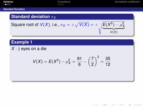
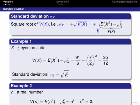
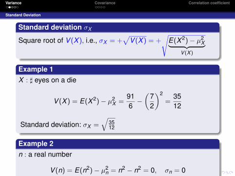
Example 1X : ] eyes on a die
V (X ) = E(X 2)− µ2X =
916−(
72
)2
=3512
Standard deviation: σX =√
3512
Example 2n : a real number
V (n) = E(n2)− µ2n = n2 − n2 = 0
,
σn = 0
beamer-tu-logo
Variance Covariance Correlation coefficient
Standard Deviation
Standard deviation σX
Square root of V (X ), i.e., σX = +√
V (X ) = +√
E(X 2)− µ2X︸ ︷︷ ︸
V (X)
Example 1X : ] eyes on a die
V (X ) = E(X 2)− µ2X =
916−(
72
)2
=3512
Standard deviation: σX =√
3512
Example 2n : a real number
V (n) = E(n2)− µ2n = n2 − n2 = 0,
σn = 0
beamer-tu-logo
Variance Covariance Correlation coefficient
Standard Deviation
Standard deviation σX
Square root of V (X ), i.e., σX = +√
V (X ) = +√
E(X 2)− µ2X︸ ︷︷ ︸
V (X)
Example 1X : ] eyes on a die
V (X ) = E(X 2)− µ2X =
916−(
72
)2
=3512
Standard deviation: σX =√
3512
Example 2n : a real number
V (n) = E(n2)− µ2n = n2 − n2 = 0, σn = 0
beamer-tu-logo
Variance Covariance Correlation coefficient
Standard Deviation
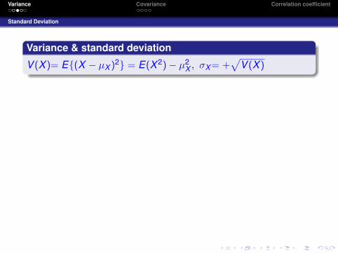
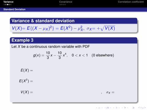
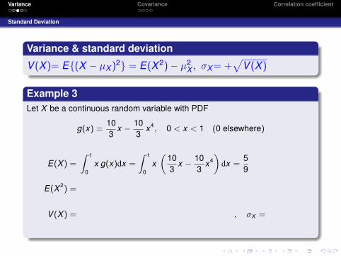
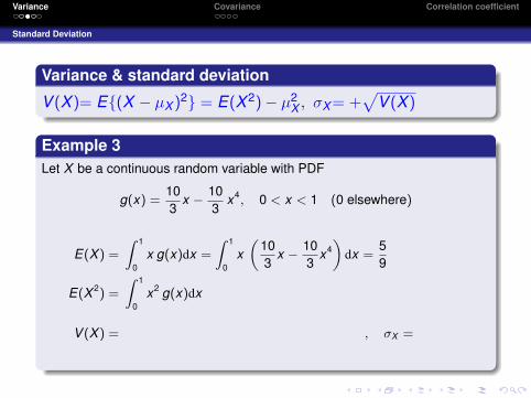
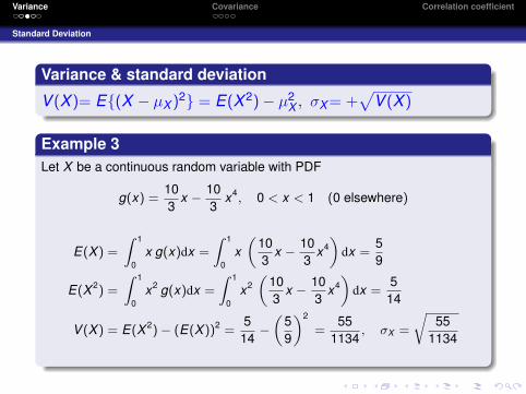
Variance & standard deviation
V (X )= E{(X − µX )2} = E(X 2)− µ2
X , σX= +√
V (X )
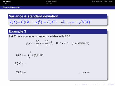
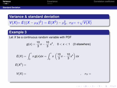
Example 3Let X be a continuous random variable with PDF
g(x) =103
x − 103
x4, 0 < x < 1 (0 elsewhere)
E(X ) =
∫ 1
0x g(x)dx =
∫ 1
0x(
103
x − 103
x4)
dx =59
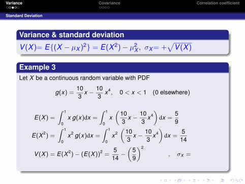
E(X 2) =
∫ 1
0x2 g(x)dx =
∫ 1
0x2(
103
x − 103
x4)
dx =5
14
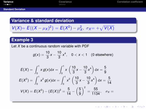
V (X ) =
E(X 2)− (E(X ))2 =5
14−(
59
)2
=55
1134
, σX =
√55
1134
beamer-tu-logo
Variance Covariance Correlation coefficient
Standard Deviation
Variance & standard deviation
V (X )= E{(X − µX )2} = E(X 2)− µ2
X , σX= +√
V (X )
Example 3Let X be a continuous random variable with PDF
g(x) =103
x − 103
x4, 0 < x < 1 (0 elsewhere)
E(X ) =
∫ 1
0x g(x)dx =
∫ 1
0x(
103
x − 103
x4)
dx =59
E(X 2) =
∫ 1
0x2 g(x)dx =
∫ 1
0x2(
103
x − 103
x4)
dx =5
14
V (X ) =
E(X 2)− (E(X ))2 =5
14−(
59
)2
=55
1134
, σX =
√55
1134
beamer-tu-logo
Variance Covariance Correlation coefficient
Standard Deviation
Variance & standard deviation
V (X )= E{(X − µX )2} = E(X 2)− µ2
X , σX= +√
V (X )
Example 3Let X be a continuous random variable with PDF
g(x) =103
x − 103
x4, 0 < x < 1 (0 elsewhere)
E(X ) =
∫ 1
0x g(x)dx
=
∫ 1
0x(
103
x − 103
x4)
dx =59
E(X 2) =
∫ 1
0x2 g(x)dx =
∫ 1
0x2(
103
x − 103
x4)
dx =5
14
V (X ) =
E(X 2)− (E(X ))2 =5
14−(
59
)2
=55
1134
, σX =
√55
1134
beamer-tu-logo
Variance Covariance Correlation coefficient
Standard Deviation
Variance & standard deviation
V (X )= E{(X − µX )2} = E(X 2)− µ2
X , σX= +√
V (X )
Example 3Let X be a continuous random variable with PDF
g(x) =103
x − 103
x4, 0 < x < 1 (0 elsewhere)
E(X ) =
∫ 1
0x g(x)dx =
∫ 1
0x(
103
x − 103
x4)
dx
=59
E(X 2) =
∫ 1
0x2 g(x)dx =
∫ 1
0x2(
103
x − 103
x4)
dx =5
14
V (X ) =
E(X 2)− (E(X ))2 =5
14−(
59
)2
=55
1134
, σX =
√55
1134
beamer-tu-logo
Variance Covariance Correlation coefficient
Standard Deviation
Variance & standard deviation
V (X )= E{(X − µX )2} = E(X 2)− µ2
X , σX= +√
V (X )
Example 3Let X be a continuous random variable with PDF
g(x) =103
x − 103
x4, 0 < x < 1 (0 elsewhere)
E(X ) =
∫ 1
0x g(x)dx =
∫ 1
0x(
103
x − 103
x4)
dx =59
E(X 2) =
∫ 1
0x2 g(x)dx =
∫ 1
0x2(
103
x − 103
x4)
dx =5
14
V (X ) =
E(X 2)− (E(X ))2 =5
14−(
59
)2
=55
1134
, σX =
√55
1134
beamer-tu-logo
Variance Covariance Correlation coefficient
Standard Deviation
Variance & standard deviation
V (X )= E{(X − µX )2} = E(X 2)− µ2
X , σX= +√
V (X )
Example 3Let X be a continuous random variable with PDF
g(x) =103
x − 103
x4, 0 < x < 1 (0 elsewhere)
E(X ) =
∫ 1
0x g(x)dx =
∫ 1
0x(
103
x − 103
x4)
dx =59
E(X 2) =
∫ 1
0x2 g(x)dx
=
∫ 1
0x2(
103
x − 103
x4)
dx =5
14
V (X ) =
E(X 2)− (E(X ))2 =5
14−(
59
)2
=55
1134
, σX =
√55
1134

beamer-tu-logo
Variance Covariance Correlation coefficient
Standard Deviation
Variance & standard deviation
V (X )= E{(X − µX )2} = E(X 2)− µ2
X , σX= +√
V (X )
Example 3Let X be a continuous random variable with PDF
g(x) =103
x − 103
x4, 0 < x < 1 (0 elsewhere)
E(X ) =
∫ 1
0x g(x)dx =
∫ 1
0x(
103
x − 103
x4)
dx =59
E(X 2) =
∫ 1
0x2 g(x)dx =
∫ 1
0x2(
103
x − 103
x4)
dx
=5
14
V (X ) =
E(X 2)− (E(X ))2 =5
14−(
59
)2
=55
1134
, σX =
√55
1134

beamer-tu-logo
Variance Covariance Correlation coefficient
Standard Deviation
Variance & standard deviation
V (X )= E{(X − µX )2} = E(X 2)− µ2
X , σX= +√
V (X )
Example 3Let X be a continuous random variable with PDF
g(x) =103
x − 103
x4, 0 < x < 1 (0 elsewhere)
E(X ) =
∫ 1
0x g(x)dx =
∫ 1
0x(
103
x − 103
x4)
dx =59
E(X 2) =
∫ 1
0x2 g(x)dx =
∫ 1
0x2(
103
x − 103
x4)
dx =5
14
V (X ) =
E(X 2)− (E(X ))2 =5
14−(
59
)2
=55
1134
, σX =
√55
1134

beamer-tu-logo
Variance Covariance Correlation coefficient
Standard Deviation
Variance & standard deviation
V (X )= E{(X − µX )2} = E(X 2)− µ2
X , σX= +√
V (X )
Example 3Let X be a continuous random variable with PDF
g(x) =103
x − 103
x4, 0 < x < 1 (0 elsewhere)
E(X ) =
∫ 1
0x g(x)dx =
∫ 1
0x(
103
x − 103
x4)
dx =59
E(X 2) =
∫ 1
0x2 g(x)dx =
∫ 1
0x2(
103
x − 103
x4)
dx =5
14
V (X ) = E(X 2)− (E(X ))2
=5
14−(
59
)2
=55
1134
, σX =
√55
1134
beamer-tu-logo
Variance Covariance Correlation coefficient
Standard Deviation
Variance & standard deviation
V (X )= E{(X − µX )2} = E(X 2)− µ2
X , σX= +√
V (X )
Example 3Let X be a continuous random variable with PDF
g(x) =103
x − 103
x4, 0 < x < 1 (0 elsewhere)
E(X ) =
∫ 1
0x g(x)dx =
∫ 1
0x(
103
x − 103
x4)
dx =59
E(X 2) =
∫ 1
0x2 g(x)dx =
∫ 1
0x2(
103
x − 103
x4)
dx =5
14
V (X ) = E(X 2)− (E(X ))2 =5
14−(
59
)2
=55
1134, σX =
√55
1134

beamer-tu-logo
Variance Covariance Correlation coefficient
Standard Deviation
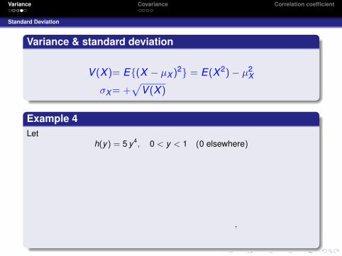
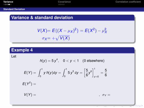
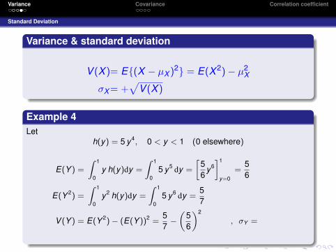
Variance & standard deviation
V (X )= E{(X − µX )2} = E(X 2)− µ2
X
σX= +√
V (X )
Example 4Let
h(y) = 5 y4, 0 < y < 1 (0 elsewhere)
E(Y ) =
∫ 1
0y h(y)dy =
∫ 1
05 y5 dy =
[56
y6]1
y=0=
56
E(Y 2) =
∫ 1
0y2 h(y)dy =
∫ 1
05 y6 dy =
57
V (Y ) = E(Y 2)− (E(Y ))2 =57−(
56
)2
=5
252
,
σY =
√5
252
beamer-tu-logo
Variance Covariance Correlation coefficient
Standard Deviation
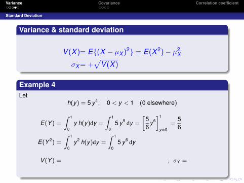
Variance & standard deviation
V (X )= E{(X − µX )2} = E(X 2)− µ2
X
σX= +√
V (X )
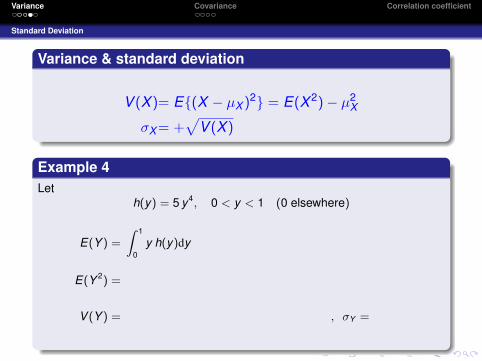
Example 4Let
h(y) = 5 y4, 0 < y < 1 (0 elsewhere)
E(Y ) =
∫ 1
0y h(y)dy =
∫ 1
05 y5 dy =
[56
y6]1
y=0=
56
E(Y 2) =
∫ 1
0y2 h(y)dy =
∫ 1
05 y6 dy =
57
V (Y ) = E(Y 2)− (E(Y ))2 =57−(
56
)2
=5
252
,
σY =
√5
252

beamer-tu-logo
Variance Covariance Correlation coefficient
Standard Deviation
Variance & standard deviation
V (X )= E{(X − µX )2} = E(X 2)− µ2
X
σX= +√
V (X )
Example 4Let
h(y) = 5 y4, 0 < y < 1 (0 elsewhere)
E(Y ) =
∫ 1
0y h(y)dy =
∫ 1
05 y5 dy =
[56
y6]1
y=0=
56
E(Y 2) =
∫ 1
0y2 h(y)dy =
∫ 1
05 y6 dy =
57
V (Y ) =
E(Y 2)− (E(Y ))2 =57−(
56
)2
=5
252
, σY =
√5
252
beamer-tu-logo
Variance Covariance Correlation coefficient
Standard Deviation
Variance & standard deviation
V (X )= E{(X − µX )2} = E(X 2)− µ2
X
σX= +√
V (X )
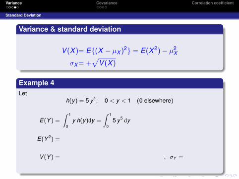
Example 4Let
h(y) = 5 y4, 0 < y < 1 (0 elsewhere)
E(Y ) =
∫ 1
0y h(y)dy
=
∫ 1
05 y5 dy =
[56
y6]1
y=0=
56
E(Y 2) =
∫ 1
0y2 h(y)dy =
∫ 1
05 y6 dy =
57
V (Y ) =
E(Y 2)− (E(Y ))2 =57−(
56
)2
=5
252
, σY =
√5
252
beamer-tu-logo
Variance Covariance Correlation coefficient
Standard Deviation
Variance & standard deviation
V (X )= E{(X − µX )2} = E(X 2)− µ2
X
σX= +√
V (X )
Example 4Let
h(y) = 5 y4, 0 < y < 1 (0 elsewhere)
E(Y ) =
∫ 1
0y h(y)dy =
∫ 1
05 y5 dy
=
[56
y6]1
y=0=
56
E(Y 2) =
∫ 1
0y2 h(y)dy =
∫ 1
05 y6 dy =
57
V (Y ) =
E(Y 2)− (E(Y ))2 =57−(
56
)2
=5
252
, σY =
√5
252

beamer-tu-logo
Variance Covariance Correlation coefficient
Standard Deviation
Variance & standard deviation
V (X )= E{(X − µX )2} = E(X 2)− µ2
X
σX= +√
V (X )
Example 4Let
h(y) = 5 y4, 0 < y < 1 (0 elsewhere)
E(Y ) =
∫ 1
0y h(y)dy =
∫ 1
05 y5 dy =
[56
y6]1
y=0
=56
E(Y 2) =
∫ 1
0y2 h(y)dy =
∫ 1
05 y6 dy =
57
V (Y ) =
E(Y 2)− (E(Y ))2 =57−(
56
)2
=5
252
, σY =
√5
252
beamer-tu-logo
Variance Covariance Correlation coefficient
Standard Deviation
Variance & standard deviation
V (X )= E{(X − µX )2} = E(X 2)− µ2
X
σX= +√
V (X )
Example 4Let
h(y) = 5 y4, 0 < y < 1 (0 elsewhere)
E(Y ) =
∫ 1
0y h(y)dy =
∫ 1
05 y5 dy =
[56
y6]1
y=0=
56
E(Y 2) =
∫ 1
0y2 h(y)dy =
∫ 1
05 y6 dy =
57
V (Y ) =
E(Y 2)− (E(Y ))2 =57−(
56
)2
=5
252
, σY =
√5
252

beamer-tu-logo
Variance Covariance Correlation coefficient
Standard Deviation
Variance & standard deviation
V (X )= E{(X − µX )2} = E(X 2)− µ2
X
σX= +√
V (X )
Example 4Let
h(y) = 5 y4, 0 < y < 1 (0 elsewhere)
E(Y ) =
∫ 1
0y h(y)dy =
∫ 1
05 y5 dy =
[56
y6]1
y=0=
56
E(Y 2) =
∫ 1
0y2 h(y)dy
=
∫ 1
05 y6 dy =
57
V (Y ) =
E(Y 2)− (E(Y ))2 =57−(
56
)2
=5
252
, σY =
√5
252
beamer-tu-logo
Variance Covariance Correlation coefficient
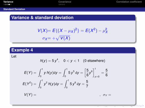
Standard Deviation
Variance & standard deviation
V (X )= E{(X − µX )2} = E(X 2)− µ2
X
σX= +√
V (X )
Example 4Let
h(y) = 5 y4, 0 < y < 1 (0 elsewhere)
E(Y ) =
∫ 1
0y h(y)dy =
∫ 1
05 y5 dy =
[56
y6]1
y=0=
56
E(Y 2) =
∫ 1
0y2 h(y)dy =
∫ 1
05 y6 dy
=57
V (Y ) =
E(Y 2)− (E(Y ))2 =57−(
56
)2
=5
252
, σY =
√5
252
beamer-tu-logo
Variance Covariance Correlation coefficient
Standard Deviation
Variance & standard deviation
V (X )= E{(X − µX )2} = E(X 2)− µ2
X
σX= +√
V (X )
Example 4Let
h(y) = 5 y4, 0 < y < 1 (0 elsewhere)
E(Y ) =
∫ 1
0y h(y)dy =
∫ 1
05 y5 dy =
[56
y6]1
y=0=
56
E(Y 2) =
∫ 1
0y2 h(y)dy =
∫ 1
05 y6 dy =
57
V (Y ) =
E(Y 2)− (E(Y ))2 =57−(
56
)2
=5
252
, σY =
√5
252
beamer-tu-logo
Variance Covariance Correlation coefficient
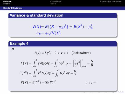
Standard Deviation
Variance & standard deviation
V (X )= E{(X − µX )2} = E(X 2)− µ2
X
σX= +√
V (X )
Example 4Let
h(y) = 5 y4, 0 < y < 1 (0 elsewhere)
E(Y ) =
∫ 1
0y h(y)dy =
∫ 1
05 y5 dy =
[56
y6]1
y=0=
56
E(Y 2) =
∫ 1
0y2 h(y)dy =
∫ 1
05 y6 dy =
57
V (Y ) = E(Y 2)− (E(Y ))2
=57−(
56
)2
=5
252
, σY =
√5
252
beamer-tu-logo
Variance Covariance Correlation coefficient
Standard Deviation
Variance & standard deviation
V (X )= E{(X − µX )2} = E(X 2)− µ2
X
σX= +√
V (X )
Example 4Let
h(y) = 5 y4, 0 < y < 1 (0 elsewhere)
E(Y ) =
∫ 1
0y h(y)dy =
∫ 1
05 y5 dy =
[56
y6]1
y=0=
56
E(Y 2) =
∫ 1
0y2 h(y)dy =
∫ 1
05 y6 dy =
57
V (Y ) = E(Y 2)− (E(Y ))2 =57−(
56
)2
=5
252
, σY =
√5
252
beamer-tu-logo
Variance Covariance Correlation coefficient
Standard Deviation
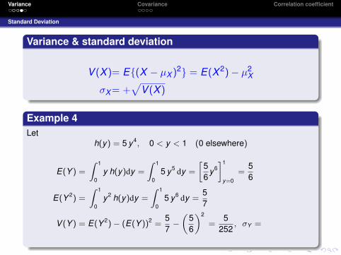
Variance & standard deviation
V (X )= E{(X − µX )2} = E(X 2)− µ2
X
σX= +√
V (X )
Example 4Let
h(y) = 5 y4, 0 < y < 1 (0 elsewhere)
E(Y ) =
∫ 1
0y h(y)dy =
∫ 1
05 y5 dy =
[56
y6]1
y=0=
56
E(Y 2) =
∫ 1
0y2 h(y)dy =
∫ 1
05 y6 dy =
57
V (Y ) = E(Y 2)− (E(Y ))2 =57−(
56
)2
=5
252, σY =
√5
252
beamer-tu-logo
Variance Covariance Correlation coefficient
Standard Deviation
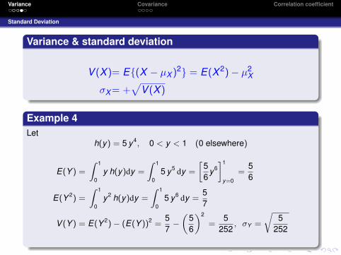
Variance & standard deviation
V (X )= E{(X − µX )2} = E(X 2)− µ2
X
σX= +√
V (X )
Example 4Let
h(y) = 5 y4, 0 < y < 1 (0 elsewhere)
E(Y ) =
∫ 1
0y h(y)dy =
∫ 1
05 y5 dy =
[56
y6]1
y=0=
56
E(Y 2) =
∫ 1
0y2 h(y)dy =
∫ 1
05 y6 dy =
57
V (Y ) = E(Y 2)− (E(Y ))2 =57−(
56
)2
=5
252, σY =
√5
252
beamer-tu-logo
Variance Covariance Correlation coefficient
Variance of linear combination of RV
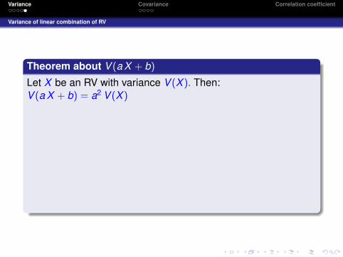
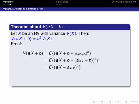
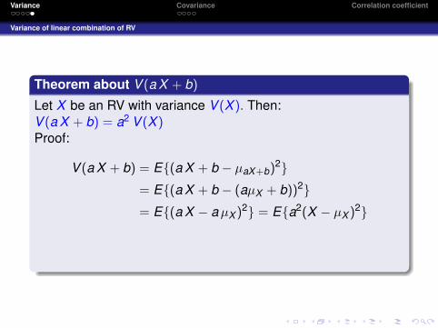
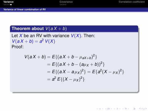
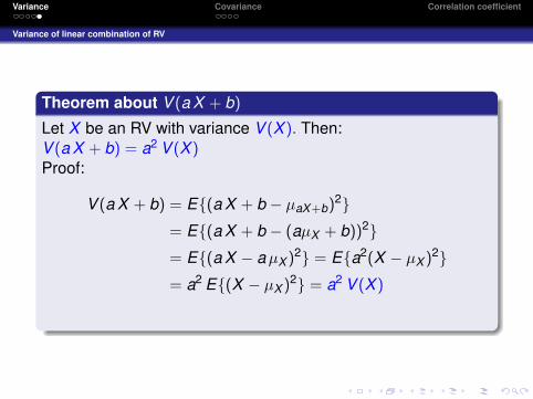
Theorem about V (a X + b)
Let X be an RV with variance V (X ). Then:V (a X + b) = a2 V (X )Proof:
V (a X + b) = E{(a X + b − µaX+b)2}
= E{(a X + b − (aµX + b))2}= E{(a X − aµX )
2} = E{a2(X − µX )2}
= a2 E{(X − µX )2} = a2 V (X )
�
beamer-tu-logo
Variance Covariance Correlation coefficient
Variance of linear combination of RV
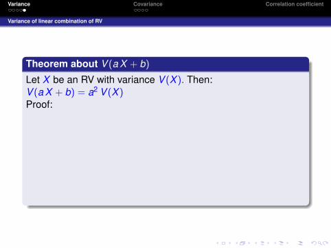
Theorem about V (a X + b)
Let X be an RV with variance V (X ). Then:V (a X + b) = a2 V (X )
Proof:
V (a X + b) = E{(a X + b − µaX+b)2}
= E{(a X + b − (aµX + b))2}= E{(a X − aµX )
2} = E{a2(X − µX )2}
= a2 E{(X − µX )2} = a2 V (X )
�
beamer-tu-logo
Variance Covariance Correlation coefficient
Variance of linear combination of RV
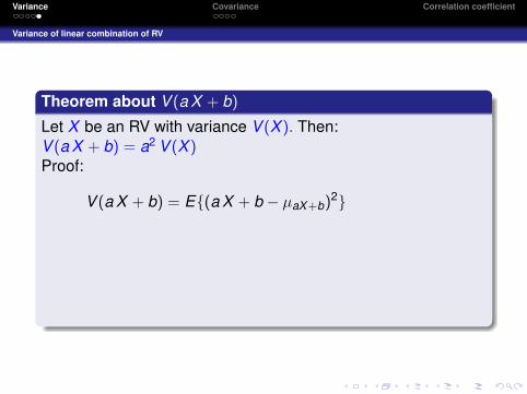
Theorem about V (a X + b)
Let X be an RV with variance V (X ). Then:V (a X + b) = a2 V (X )Proof:
V (a X + b) = E{(a X + b − µaX+b)2}
= E{(a X + b − (aµX + b))2}= E{(a X − aµX )
2} = E{a2(X − µX )2}
= a2 E{(X − µX )2} = a2 V (X )
�
beamer-tu-logo
Variance Covariance Correlation coefficient
Variance of linear combination of RV
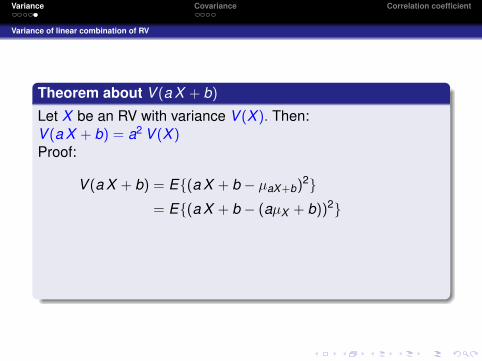
Theorem about V (a X + b)
Let X be an RV with variance V (X ). Then:V (a X + b) = a2 V (X )Proof:
V (a X + b) = E{(a X + b − µaX+b)2}
= E{(a X + b − (aµX + b))2}= E{(a X − aµX )
2} = E{a2(X − µX )2}
= a2 E{(X − µX )2} = a2 V (X )
�
beamer-tu-logo
Variance Covariance Correlation coefficient
Variance of linear combination of RV
Theorem about V (a X + b)
Let X be an RV with variance V (X ). Then:V (a X + b) = a2 V (X )Proof:
V (a X + b) = E{(a X + b − µaX+b)2}
= E{(a X + b − (aµX + b))2}
= E{(a X − aµX )2} = E{a2(X − µX )
2}= a2 E{(X − µX )
2} = a2 V (X )
�
beamer-tu-logo
Variance Covariance Correlation coefficient
Variance of linear combination of RV
Theorem about V (a X + b)
Let X be an RV with variance V (X ). Then:V (a X + b) = a2 V (X )Proof:
V (a X + b) = E{(a X + b − µaX+b)2}
= E{(a X + b − (aµX + b))2}= E{(a X − aµX )
2}
= E{a2(X − µX )2}
= a2 E{(X − µX )2} = a2 V (X )
�
beamer-tu-logo
Variance Covariance Correlation coefficient
Variance of linear combination of RV
Theorem about V (a X + b)
Let X be an RV with variance V (X ). Then:V (a X + b) = a2 V (X )Proof:
V (a X + b) = E{(a X + b − µaX+b)2}
= E{(a X + b − (aµX + b))2}= E{(a X − aµX )
2} = E{a2(X − µX )2}
= a2 E{(X − µX )2} = a2 V (X )
�
beamer-tu-logo
Variance Covariance Correlation coefficient
Variance of linear combination of RV
Theorem about V (a X + b)
Let X be an RV with variance V (X ). Then:V (a X + b) = a2 V (X )Proof:
V (a X + b) = E{(a X + b − µaX+b)2}
= E{(a X + b − (aµX + b))2}= E{(a X − aµX )
2} = E{a2(X − µX )2}
= a2 E{(X − µX )2}
= a2 V (X )
�
beamer-tu-logo
Variance Covariance Correlation coefficient
Variance of linear combination of RV
Theorem about V (a X + b)
Let X be an RV with variance V (X ). Then:V (a X + b) = a2 V (X )Proof:
V (a X + b) = E{(a X + b − µaX+b)2}
= E{(a X + b − (aµX + b))2}= E{(a X − aµX )
2} = E{a2(X − µX )2}
= a2 E{(X − µX )2} = a2 V (X )
�
beamer-tu-logo
Variance Covariance Correlation coefficient
And now . . .
1 VarianceDefinitionStandard DeviationVariance of linear combination of RV
2 CovarianceMeaning & DefinitionExamples
3 Correlation coefficient
beamer-tu-logo
Variance Covariance Correlation coefficient
Meaning & Definition
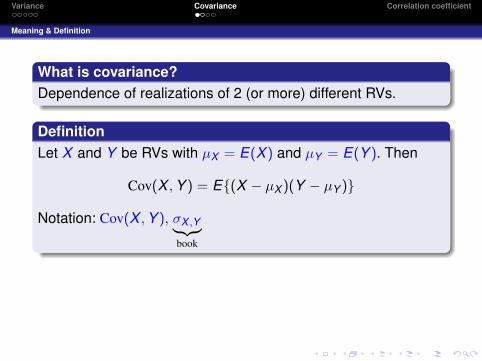
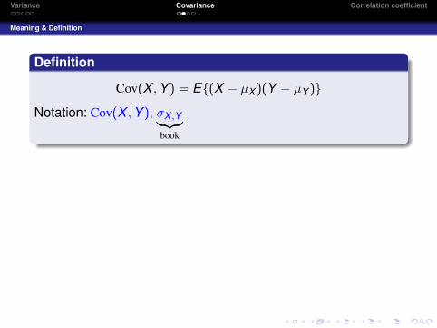
What is covariance?Dependence of realizations of 2 (or more) different RVs.
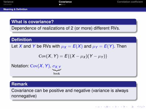
DefinitionLet X and Y be RVs with µX = E(X ) and µY = E(Y ). Then
Cov(X ,Y ) = E{(X − µX )(Y − µY )}
Notation: Cov(X ,Y ), σX ,Y︸︷︷︸book
RemarkCovariance can be positive and negative (variance is alwaysnonnegative)
beamer-tu-logo
Variance Covariance Correlation coefficient
Meaning & Definition
What is covariance?Dependence of realizations of 2 (or more) different RVs.
DefinitionLet X and Y be RVs with µX = E(X ) and µY = E(Y ). Then
Cov(X ,Y ) = E{(X − µX )(Y − µY )}
Notation: Cov(X ,Y ), σX ,Y︸︷︷︸book
RemarkCovariance can be positive and negative (variance is alwaysnonnegative)
beamer-tu-logo
Variance Covariance Correlation coefficient
Meaning & Definition
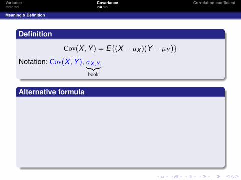
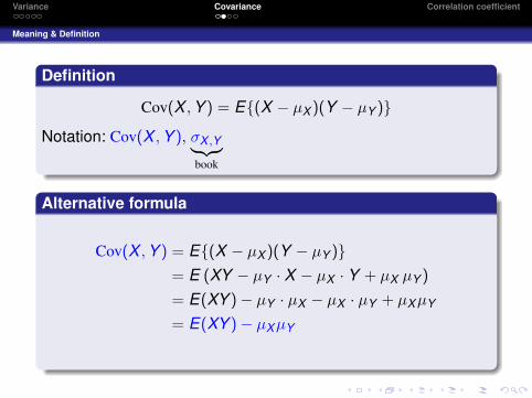
Definition
Cov(X ,Y ) = E{(X − µX )(Y − µY )}
Notation: Cov(X ,Y ), σX ,Y︸︷︷︸book
Alternative formula
Cov(X ,Y ) = E{(X − µX )(Y − µY )}= E (XY − µY · X − µX · Y + µX µY )
= E(XY )− µY · µX − µX · µY + µXµY
= E(XY )− µXµY
beamer-tu-logo
Variance Covariance Correlation coefficient
Meaning & Definition
Definition
Cov(X ,Y ) = E{(X − µX )(Y − µY )}
Notation: Cov(X ,Y ), σX ,Y︸︷︷︸book
Alternative formula
Cov(X ,Y ) = E{(X − µX )(Y − µY )}= E (XY − µY · X − µX · Y + µX µY )
= E(XY )− µY · µX − µX · µY + µXµY
= E(XY )− µXµY
beamer-tu-logo
Variance Covariance Correlation coefficient
Examples
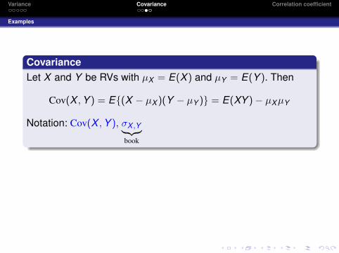
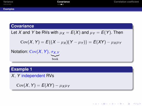
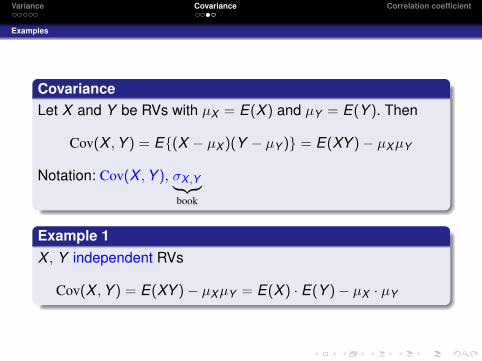
CovarianceLet X and Y be RVs with µX = E(X ) and µY = E(Y ). Then
Cov(X ,Y ) = E{(X − µX )(Y − µY )} = E(XY )− µXµY
Notation: Cov(X ,Y ), σX ,Y︸︷︷︸book
Example 1X , Y independent RVs
Cov(X ,Y ) = E(XY )− µXµY = E(X ) · E(Y )− µX · µY = 0

beamer-tu-logo
Variance Covariance Correlation coefficient
Examples
CovarianceLet X and Y be RVs with µX = E(X ) and µY = E(Y ). Then
Cov(X ,Y ) = E{(X − µX )(Y − µY )} = E(XY )− µXµY
Notation: Cov(X ,Y ), σX ,Y︸︷︷︸book
Example 1X , Y independent RVs
Cov(X ,Y )
= E(XY )− µXµY = E(X ) · E(Y )− µX · µY = 0
beamer-tu-logo
Variance Covariance Correlation coefficient
Examples
CovarianceLet X and Y be RVs with µX = E(X ) and µY = E(Y ). Then
Cov(X ,Y ) = E{(X − µX )(Y − µY )} = E(XY )− µXµY
Notation: Cov(X ,Y ), σX ,Y︸︷︷︸book
Example 1X , Y independent RVs
Cov(X ,Y ) = E(XY )− µXµY
= E(X ) · E(Y )− µX · µY = 0
beamer-tu-logo
Variance Covariance Correlation coefficient
Examples
CovarianceLet X and Y be RVs with µX = E(X ) and µY = E(Y ). Then
Cov(X ,Y ) = E{(X − µX )(Y − µY )} = E(XY )− µXµY
Notation: Cov(X ,Y ), σX ,Y︸︷︷︸book
Example 1X , Y independent RVs
Cov(X ,Y ) = E(XY )− µXµY = E(X ) · E(Y )− µX · µY
= 0

beamer-tu-logo
Variance Covariance Correlation coefficient
Examples
CovarianceLet X and Y be RVs with µX = E(X ) and µY = E(Y ). Then
Cov(X ,Y ) = E{(X − µX )(Y − µY )} = E(XY )− µXµY
Notation: Cov(X ,Y ), σX ,Y︸︷︷︸book
Example 1X , Y independent RVs
Cov(X ,Y ) = E(XY )− µXµY = E(X ) · E(Y )− µX · µY = 0
beamer-tu-logo
Variance Covariance Correlation coefficient
Examples
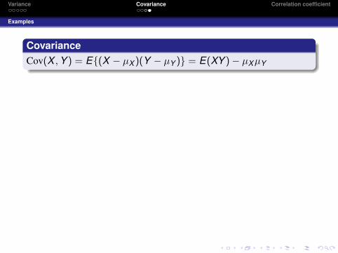
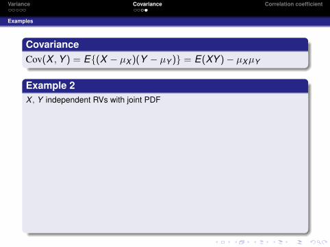
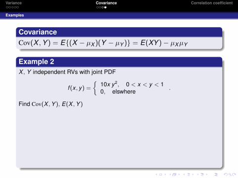
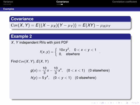
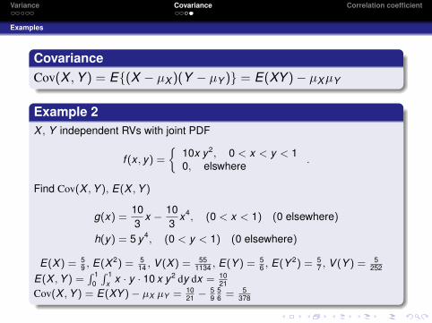
CovarianceCov(X ,Y ) = E{(X − µX )(Y − µY )} = E(XY )− µXµY
Example 2X , Y independent RVs with joint PDF
f (x , y) ={
10x y2, 0 < x < y < 10, elswhere
.
Find Cov(X ,Y ), E(X ,Y )
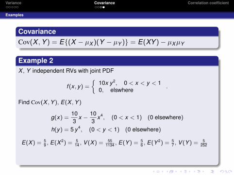
g(x) =103
x − 103
x4, (0 < x < 1) (0 elsewhere)
h(y) = 5 y4, (0 < y < 1) (0 elsewhere)
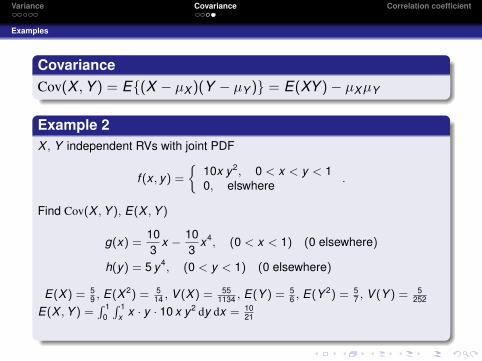
E(X ) = 59 , E(X 2) = 5
14 , V (X ) = 551134 , E(Y ) = 5
6 , E(Y 2) = 57 , V (Y ) = 5
252
E(X ,Y ) =∫ 1
0
∫ 1x x · y · 10 x y2 dy dx = 10
21Cov(X ,Y ) = E(XY )− µX µY = 10
21 − 59
56 = 5
378
beamer-tu-logo
Variance Covariance Correlation coefficient
Examples
CovarianceCov(X ,Y ) = E{(X − µX )(Y − µY )} = E(XY )− µXµY
Example 2X , Y independent RVs with joint PDF
f (x , y) ={
10x y2, 0 < x < y < 10, elswhere
.
Find Cov(X ,Y ), E(X ,Y )
g(x) =103
x − 103
x4, (0 < x < 1) (0 elsewhere)
h(y) = 5 y4, (0 < y < 1) (0 elsewhere)
E(X ) = 59 , E(X 2) = 5
14 , V (X ) = 551134 , E(Y ) = 5
6 , E(Y 2) = 57 , V (Y ) = 5
252
E(X ,Y ) =∫ 1
0
∫ 1x x · y · 10 x y2 dy dx = 10
21
Cov(X ,Y ) = E(XY )− µX µY = 1021 − 5
956 = 5
378
beamer-tu-logo
Variance Covariance Correlation coefficient
Examples
CovarianceCov(X ,Y ) = E{(X − µX )(Y − µY )} = E(XY )− µXµY
Example 2X , Y independent RVs with joint PDF
f (x , y) ={
10x y2, 0 < x < y < 10, elswhere
.
Find Cov(X ,Y ), E(X ,Y )
g(x) =103
x − 103
x4, (0 < x < 1) (0 elsewhere)
h(y) = 5 y4, (0 < y < 1) (0 elsewhere)
E(X ) = 59 , E(X 2) = 5
14 , V (X ) = 551134 , E(Y ) = 5
6 , E(Y 2) = 57 , V (Y ) = 5
252
E(X ,Y ) =∫ 1
0
∫ 1x x · y · 10 x y2 dy dx = 10
21Cov(X ,Y ) = E(XY )− µX µY = 10
21 − 59
56 = 5
378
beamer-tu-logo
Variance Covariance Correlation coefficient
And now . . .
1 VarianceDefinitionStandard DeviationVariance of linear combination of RV
2 CovarianceMeaning & DefinitionExamples
3 Correlation coefficient

beamer-tu-logo
Variance Covariance Correlation coefficient
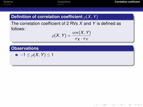
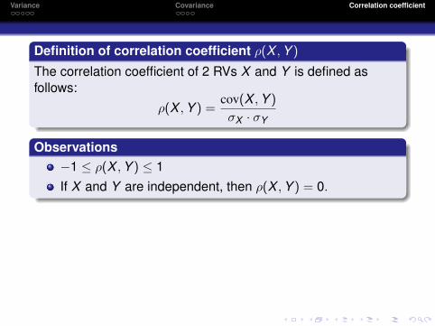
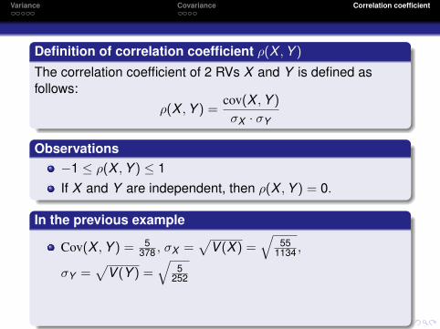
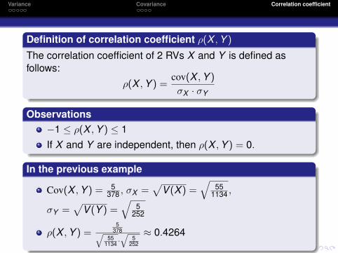
Definition of correlation coefficient ρ(X ,Y )
The correlation coefficient of 2 RVs X and Y is defined asfollows:
ρ(X ,Y ) =cov(X ,Y )
σX · σY
Observations−1 ≤ ρ(X ,Y ) ≤ 1
If X and Y are independent, then ρ(X ,Y ) = 0.
In the previous example
Cov(X ,Y ) = 5378 , σX =
√V (X ) =
√55
1134 ,
σY =√
V (Y ) =√
5252
ρ(X ,Y ) =5
378√55
1134 ·√
5252
≈ 0.4264
beamer-tu-logo
Variance Covariance Correlation coefficient
Definition of correlation coefficient ρ(X ,Y )
The correlation coefficient of 2 RVs X and Y is defined asfollows:
ρ(X ,Y ) =cov(X ,Y )
σX · σY
Observations−1 ≤ ρ(X ,Y ) ≤ 1If X and Y are independent, then ρ(X ,Y ) = 0.
In the previous example
Cov(X ,Y ) = 5378 , σX =
√V (X ) =
√55
1134 ,
σY =√
V (Y ) =√
5252
ρ(X ,Y ) =5
378√55
1134 ·√
5252
≈ 0.4264