EigenFaces

(squared) Variance

• A measure of how "spread out" a sequence of numbers are.

Covariance matrix

• A measure of correlation between data elements.

• Example:– Data set of size n– Each data element has 3 fields:• Height• Weight• Birth date

Covariance

• [Collect data from class]

Covariance

Covariance

• The diagonals are the variance of that feature• Non-diagonals are a measure of correlation– High-positive == positive correlation• one goes up, other goes up

– Low-negative == negative correlation• one goes up, other goes down

– Near-zero == no correlation• unrelated

– [How high depends on the range of values]

Covariance

• You can calculate it with a matrix:– Raw Matrix is a p x q matrix• p features• q samples

– Convert to mean-deviation form• Calculate the average sample• Subtract this from all samples.

– Multiply MeanDev (a p x q matrix) by its transpose (a q x p matrix)

– Multiply by 1/n to get the covariance matrix.

Covariance

• [Calculate our covariance matrix]

EigenSystems

• An EigenSystem is:A vector (the eigenvector)A scalar λ (the eigenvalue)

• Such that:

(the zero vector isn't an eigenvector)• In general, not all matrices have eigenvectors.

EigenSystems and PCA

• When you calculate the eigen-system of an n x n Covariance matrix you get:– n eigenvectors (each of dimension n)– n matching eigenvalues

• The biggest eigen-value "explains" the largest amount of variance in the data set.

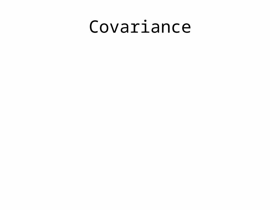
Example• Say we have a 2d data set

– First eigen-pair (v1 = [0.8, 0.6], λ=800.0)– Second eigen-pair (v2 = [-0.6, 0.8], λ=100.0)– 8x as much variance is along v1 as v2.– v1 and v2 are perpendicular to each other– v1 and v2 define a new set of basis vectors for this data set.

v1

v2

Conversions between basis vectors• Let's take one data point…

– Let's say it is [-1.5, 0.4] in "world units"• Project it onto v1 and v2 to get the

coordinates relative to (v1, v2 unit-length basis vectors)

v1

v2

To convert back to "world units":

PCA and compression

• Example:– n (the number of features) is high (~100)– Most of the variance is captured by 3 eigen-

vectors.– You can throw out the other 97 eigen-vectors.– You can represent most of the data for each

sample using just 3 numbers per sample (instead of 100)• For a large data set, this can be huge.

EigenFaces

1. Collect database imagesa. Subject looking straight ahead, no emotion,

neutral lighting.b. Crop:

i. on the top include all of the eyebrowsii. on the bottom include just to the chiniii. on the sides, include all of the face.

c. Size to 32x32, grayscale (a limit of the eigen-solver)d. In code, include a way to convert to (and from) a

VectorN.

EigenFaces, cont.

2. Calculate the average imagea. Just pixel (Vector element) by element.

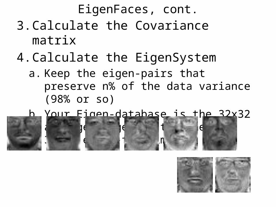
EigenFaces, cont.3. Calculate the Covariance matrix4. Calculate the EigenSystem

a. Keep the eigen-pairs that preserve n% of the data variance (98% or so)

b. Your Eigen-database is the 32x32 average image and the (here) 8 32x32 eigen-face images.

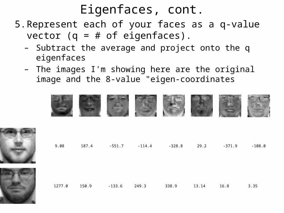
Eigenfaces, cont.5. Represent each of your faces as a q-value vector (q

= # of eigenfaces).– Subtract the average and project onto the q eigenfaces– The images I'm showing here are the original image

and the 8-value "eigen-coordinates

9.08 187.4 -551.7 -114.4 -328.8 29.2 -371.9 -108.0

1277.0 150.9 -133.6 249.3 338.9 13.14 16.8 3.35

EigenFaces, cont.6. (for demonstration of compression) – You can reconstruct a compressed image by:• Start with a copy of the average image, X• Repeat for each eigenface:

– Add the eigen-coord * eigenface to X

– Here are the reconstructions of the 2 images on the last slide: Original Reconstruction

EigenFaces, cont.7. Facial Recognition– Take a novel image (same size as database

images)– Using the eigenfaces computed earlier (this novel

image is usually NOT part of this computation), compute eigen-coordinates.

– Calculate the q-dimensional distance (pythagorean theorem in q-dimensions) between this image and each database image.• The database image with the smallest distance is your

best match.