Lecture 7.1 Epipolar geometry

Thomas Opsahl

Weekly overview – Two-view geometry

• Epipolar geometry – Algebraic representation & estimation – The essential matrix – The fundamental matrix

• Triangulation

– Sparse 3D scene reconstructing from 2D correspondences

• Relative pose from epipolar geometry

– Estimating the relative pose from the essential matrix

– Visual odometry

2

Introduction

• Observing the same points in two views puts a strong geometrical constraint on the cameras

• Algebraically this epipolar constraint is usually

represented by two related 3 × 3 matrices

3

𝑿

𝒖 𝒖𝒖

𝐶

𝒙 𝒙𝒖

𝐶𝒖

Introduction

• Observing the same points in two views puts a strong geometrical constraint on the cameras

• Algebraically this epipolar constraint is usually

represented by two related 3 × 3 matrices

• The fundamental matrix 𝐹 𝒖�𝒖𝑇𝐹𝒖�

• The essential matrix 𝐸

𝒙�𝒖𝑇𝐸𝒙�

• These are coupled through the two calibration matrices 𝐾 and 𝐾𝒖

4

𝒖 𝒖𝒖

𝐶

𝒙 𝒙𝒖

𝐶𝒖

𝑿

𝐹

𝐾 𝐾𝒖

𝐸

The essential matrix E

• Let 𝒙𝐶 ↔ 𝒙𝒖𝐶𝐶 be corresponding points in the normalized image planes and let the pose of 𝐶 relative to 𝐶𝒖 be

𝜉𝐶𝐶𝐶 = 𝑅 𝒕𝟎 1

5

𝒕

𝒙𝐶

𝒙𝒖𝐶𝐶

𝐶

𝐶𝒖

The essential matrix E

• Let 𝒙𝐶 ↔ 𝒙𝒖𝐶𝐶 be corresponding points in the normalized image planes and let the pose of 𝐶 relative to 𝐶𝒖 be

𝜉𝐶𝐶𝐶 = 𝑅 𝒕𝟎 1

• In terms of vectors, the equation for the epipolar

plane can be written like 𝒙�𝒖𝐶𝐶 × 𝒕 ∙ 𝑅 𝒙�𝐶 = 0

• Rewritten in terms of matrices this takes the form

𝒙�𝒖𝑇𝐶𝐶 𝒕 ×𝑅 𝒙�𝐶 = 0

• This relationship defines the essential matrix 𝐸 = 𝒕 ×𝑅

6

𝒙�𝒖𝑇𝐸𝒙� = 0

𝒙𝐶

𝒙𝒖𝐶𝐶

𝐶

𝐶𝒖

𝒕 𝒙�𝒖𝐶𝐶

𝒙�𝐶

The essential matrix E

• The essential matrix 𝐸 represents the epipolar constraint on corresponding normalized points

• Note that although 𝒙�𝒖𝑇𝐸𝒙� = 0 is a necessary requirement for the correspondence 𝒙 ↔ 𝒙𝒖 to be geometrically possible, it does not guarantee its correctness

8

𝒙𝐶

𝒙𝒖𝐶𝐶

𝐶

𝐶𝒖

𝒕 𝒙�𝒖𝐶𝐶

𝒙�𝐶

The essential matrix E

• Properties of 𝐸 – 𝐸 = 𝒕 ×𝑅 – Homogeneous – 𝑟𝑟𝑟𝑟 = 2 – det = 0 – 5 degrees of freedom – 𝐸 can be estimated from a minimum of 5

point correspondences – If 𝒙 and 𝒙𝒖 are corresponding normalized

image points, then 𝒙�𝒖𝑇𝐸𝒙� = 0 – 𝐸 has 2 singular values that are equal and

a third that is zero

• It is possible to decompose 𝐸 = 𝒕 ×𝑅 to determine the relative pose between cameras – Translation only up to scale – Topic of another lecture

9

𝐶

𝒙 𝒙𝒖

𝐶𝒖

𝑿

𝐸

The fundamental matrix F

• The epipolar constraint on image points is naturally connected to the essential matrix by the calibration matrices 𝐾 and 𝐾𝒖

• Combined with the epipolar constraint for normalized image points we get

• This defines the fundamental matrix 𝐹 = 𝐾𝒖−𝑇𝐸𝐾−1

10

1

1

C C

C C C T T T

K KK K K

−

′ ′ ′− −

= ⇒ =

′ ′ ′ ′ ′ ′ ′ ′ ′= ⇒ = ⇒ =

x u x ux u x u x u

1

00

C T C

T T

EK EK

′

− −

′ =

′ ′ =

x xu u

𝒖�𝒖𝑇𝐹𝒖� = 0

𝒖 𝒖𝒖

𝐶

𝒙 𝒙𝒖

𝐶𝒖

𝑿

𝐹

𝐾 𝐾𝒖

𝐸

The fundamental matrix F

• Properties of 𝐹 – 𝐹 = 𝐾𝒖−𝑇𝐸𝐾−1 – Homogeneous – 𝑟𝑟𝑟𝑟 = 2 – det = 0 – 7 degrees of freedom – 𝐹 can be estimated from a minimum of 7 point

correspondences – If 𝒖 and 𝒖𝒖 are corresponding image points, then

𝒖�𝒖𝑇𝐹𝒖� = 0 – For any point 𝒖 in image 1, the corresponding

epipolar line 𝒍𝒖 in image 2 is given by �̃�𝒖 = 𝐹𝒖�

– For any point 𝒖𝒖 in image 2, the corresponding

epipolar line 𝒍 in image 1 is given by �̃� = 𝐹𝑇𝒖�𝒖

– The epipole 𝒆𝒖 in image 2 is 𝐹’s left singular vector corresponding to the zero singular value

– The epipole 𝒆 in image 1 is 𝐹’s right singular vector corresponding to the zero singular value

11

𝒖 𝒖𝒖

𝐶

𝒙 𝒙𝒖

𝐶𝒖

𝑿

𝐹

𝐾 𝐾𝒖

Example

• These fundamental lines were determined using the fundamental matrix between images • Recall that points and lines are dual in ℙ2

12

𝒖

𝒖𝒖

[ ]0 1 2 0 1 20 0 01

T

ul l l v l u l v l

= ⇔ = ⇔ + + =

l u

Estimating F

• Several algorithms – Non-iterative: 7-pt, 8-pt – Iterative: Minimize epipolar error – Robust: RANSAC with 7-pt

• From the definition it follows that each point

correspondence 𝒖𝑖 ↔ 𝒖𝑖𝒖 contributes with 1 equation

• So given several correspondences we get a homogeneous system of linear equations that we can solve by SVD

• As before, we see that the matrix A contains terms that can be very different in scale, so point sets 𝒖𝑖 and 𝒖𝑖𝒖 should be normalized in advance

– Centroids origin – Mean distance from origin should be 2

13

[ ]

[ ]

1 2 3

4 5 6

7 8 9

0

1 01

1 0

Ti i

i

i i i

i i i i i i i i i i i i

Ff f f u

u v f f f vf f f

u u u v u u v v v v u v

′ =

′ ′ =

′ ′ ′ ′ ′ ′ =

u u

f

1 1 1 1 1 1 1 1 1 1 1 1 10

10

n n n n n n n n n n n n

u u u v u u v v v v u v

u u u v u u v v v v u vA

′ ′ ′ ′ ′ ′ =

′ ′ ′ ′ ′ ′ =

f

f

Estimating F The normalized 8-point algorithm Given 𝑟 ≥ 8 correspondences 𝒖𝑖 ↔ 𝒖𝑖𝒖, do the following

1. Normalize points 𝒖𝑖 and 𝒖𝑖𝒖 usingsimilarity

transforms 𝑇 and 𝑇𝒖 2. Build matrix 𝐴 from point-correspondences and

compute its SVD 3. Extract the “solution” 𝐹� from the right singular

vector corresponding to the smallest singular value

4. Compute the SVD of 𝐹�: 𝐹� = 𝑈𝑈𝑉𝑇 5. Enforce zero determinant by setting 𝑠33 = 0 and

compute a proper fundamental matrix 𝐹� = 𝑈𝑈𝑉𝑇

6. Denormalize 𝐹 = 𝑇𝒖𝑇𝐹�𝑇

14

𝒖 𝒖𝒖

𝐶

𝒙 𝒙𝒖

𝐶𝒖

𝑿

𝐹

𝐾 𝐾𝒖

𝒖� 𝒖�𝒖 𝐹�

𝑇 𝑇𝒖

( ) ( )

ˆˆ ˆ 0ˆ ˆ0

ˆ 0

T

T T

T T

F

T F T F T FT

T FT

′ =

′ ′ ′= ⇒ =

′ ′ =

u u

u u

u u

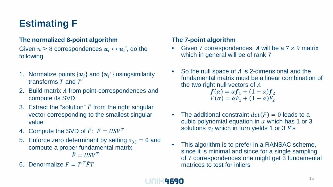
Estimating F The normalized 8-point algorithm Given 𝑟 ≥ 8 correspondences 𝒖𝑖 ↔ 𝒖𝑖𝒖, do the following

1. Normalize points 𝒖𝑖 and 𝒖𝑖𝒖 usingsimilarity

transforms 𝑇 and 𝑇𝒖 2. Build matrix 𝐴 from point-correspondences and

compute its SVD 3. Extract the “solution” 𝐹� from the right singular

vector corresponding to the smallest singular value

4. Compute the SVD of 𝐹�: 𝐹� = 𝑈𝑈𝑉𝑇 5. Enforce zero determinant by setting 𝑠33 = 0 and

compute a proper fundamental matrix 𝐹� = 𝑈𝑈𝑉𝑇

6. Denormalize 𝐹 = 𝑇𝒖𝑇𝐹�𝑇

15

The 7-point algorithm • Given 7 correspondences, 𝐴 will be a 7 × 9 matrix

which in general will be of rank 7

• So the null space of 𝐴 is 2-dimensional and the fundamental matrix must be a linear combination of the two right null vectors of 𝐴

𝒇 𝛼 = 𝛼𝒇1 + 1 − 𝛼 𝒇2 𝐹 𝛼 = 𝛼𝐹1 + 1 − 𝛼 𝐹2

• The additional constraint 𝑑𝑑𝑑 𝐹 = 0 leads to a

cubic polynomial equation in 𝛼 which has 1 or 3 solutions 𝛼𝑖 which in turn yields 1 or 3 𝐹’s

• This algorithm is to prefer in a RANSAC scheme, since it is minimal and since for a single sampling of 7 correspondences one might get 3 fundamental matrices to test for inliers

Estimating F • Improved estimates of 𝐹 can be obtained using

iterative methods like Levenberg-Marquardt to minimize the epipolar error

𝜖 = �𝑑 𝒖�,𝐹𝑇𝒖�𝒖 + 𝑑 𝒖�𝒖,𝐹𝒖�

16

• OpenCV – cv::Mat cv::findFundamentalMat – Arguments are

InputArray points1 InputArray points2 int method – {CV_FM_7POINT, CV_FM_8POINT, CV_FM_RANSAC, CV_FM_LMEDS} double param1 double param2 OutputArray mask

• Matlab

– estimateFundamentalMatrix

𝒖 𝒖𝒖

𝐹

�̃�𝒖 = 𝐹𝒖� �̃� = 𝐹𝑇𝒖�𝒖

Estimating F • Improved estimates of 𝐹 can be obtained using

iterative methods like Levenberg-Marquardt to minimize the epipolar error

𝜖 = �𝑑 𝒖�,𝐹𝑇𝒖�𝒖 + 𝑑 𝒖�𝒖,𝐹𝒖�

• Distance between homogeneous point 𝒖� and line �̃� = 𝑙1, 𝑙2, 𝑙3

𝑻

17

• OpenCV – cv::Mat cv::findFundamentalMat – Arguments are

InputArray points1 InputArray points2 int method – {CV_FM_7POINT, CV_FM_8POINT, CV_FM_RANSAC, CV_FM_LMEDS} double param1 double param2 OutputArray mask

• Matlab

– estimateFundamentalMatrix

𝒖 𝒖𝒖

𝐹

�̃�𝒖 = 𝐹𝒖� �̃� = 𝐹𝑇𝒖�𝒖

𝑑 𝒖�,𝐹𝑇𝒖�𝒖 𝑑 𝒖�𝒖,𝐹𝒖�

( )2 2

1 2

,T

dl l

=+

u lu l

Estimating E

• For calibrated cameras (𝐾 and 𝐾𝒖 are known), we can first estimate 𝐹 and then compute 𝐸 = 𝐾𝒖𝑇𝐹𝐾

• It is also possible to estimate 𝐸 directly from 5

normalized point correspondences 𝒙𝑖 ↔ 𝒙𝑖𝒖 – Algorithm proposed by David Nistér in 2004 – Involves finding the roots of a 10th degree

polynomial

• In RANSAC schemes, the 5-point algorithm is the fastest alternative

– To acieve 99% confidence with 50% outliers, the 5-point algorithm only requires 145 tests while the 8-point algorithm requires 1177 tests

• OpenCV – cv::Mat cv::findEssentialMat – 5-pt algorithm

• Matlab

– Currently not available as a built in function in Matlab

– MexOpenCV

• OpenGV: http://laurentkneip.github.io/opengv/ contains several interesting functions

– 5-pt algorithm – 2-pt algorithm based on known relative rotation

18

Summary

• Algebraic representation of epipolar geometry – The essential matrix – The fundamental matrix

• Estimating the epipolar geometry

– Estimate 𝐹: 7pt, 8pt, RANSAC – Estimate 𝐸: 5pt

• Additional reading:

– Szeliski: 7.2

19

𝒖 𝒖𝒖

𝐶

𝒙 𝒙𝒖

𝐶𝒖

𝑿

𝐹

𝐾 𝐾𝒖

𝐸