Lecture 5: Intermediate macroeconomics, autumn 2008perseus.iies.su.se/~calmf/Ekonomisk...

Lecture 5: Intermediate macroeconomics, autumn 2008 Lars Calmfors

1 1

Purchasing power parity – PPP

Theory of determination of the exchange rate in the long

run, which emphasises the importance of goods markets

(in contrast to asset markets)

Gustaf Cassel (1866 – 1945)

Law of one price

$/€

$/€

/

i iEUS

i iEUS

P E P

E P P

=

=

g

Absolute purchasing power parity

/€ EEPP= $/€ / EUSE P P=

Relative purchasing power parity

, , $/€, $/€, -1 $/€, -1

-1 -1

( ) /

( ) /

E tUS tt t t

t t t t

E E E

P P P

π π

π

− = −

= −

Fig. 15-2: The Yen/Dollar Exchange Rate and Relative Japan-U.S. Price Levels, 1980–2006

Source: IMF, International Financial Statistics. Exchange rates and price levels are end-of-year data.

3

Causes of deviations from PPP

1. Transport costs and trade barriers

2. Differences in consumption baskets

3. Imperfect competition – price discrimination - pricing to

market

Different PPP exchange rates depending on which country’s

consumption basket is used

/US GP P is higher with German basket than with US basket,

because goods that are relatively cheap in the US have a larger

weight in the American than in the German basket.

Different types of goods and services

• Tradables or traded goods

• Non-tradables or non-traded goods (primarily services and

building)

4

EEAG Report 2008

Fig. 1.5 Exchange rates of the euro and PPPs

Sources: European Central Bank, Federal Statistical Office, OECD and calculations by the Ifo Institute.

0.60

0.70

0.80

0.90

1.00

1.10

1.20

1.30

1.40

1.50USD per EUR

OECD basket

US basket

German basket

Jan.

90 91 92 93 94 95 96 97 98 99 00 01 02 03 04 05 06 07 08

Exchange rate

a) The exchange rate is based on monthly data, while PPPs are given at an annual frequency. Different PPPsare computed with respect to the different consumption baskets in the United States, the OECD and Germany.See footnote 8, Chapter 1, EEAG (2005).

5

The Balassa-Samuelson-effect

The price level is higher in countries with high per capita income,

because prices of non-tradables are higher.

(1) PEP= TT PP E ∗= (international goods arbitrage)

(2) T TTW P MPL⋅= (profit maximisation in tradables sector)

(3) TNW W= (homogenous labour market)

(4) /N N NP W MPL= (price = marginal cost for

non-tradables)

(5) 1 T NCP P Pα α−= (consumer price index)

The Balassa-Samuelson effect implies a higher relative price for

non-tradables in rich than in poor countries:

1 1

N N T T T TT T N T N T N N

NTN T

P W W P MPL MPLP P MPL P MPL P MPL MPL

PMPLMPL P

⋅= ⋅ = ⋅ = =⋅

↑ ⇒ ↑

6

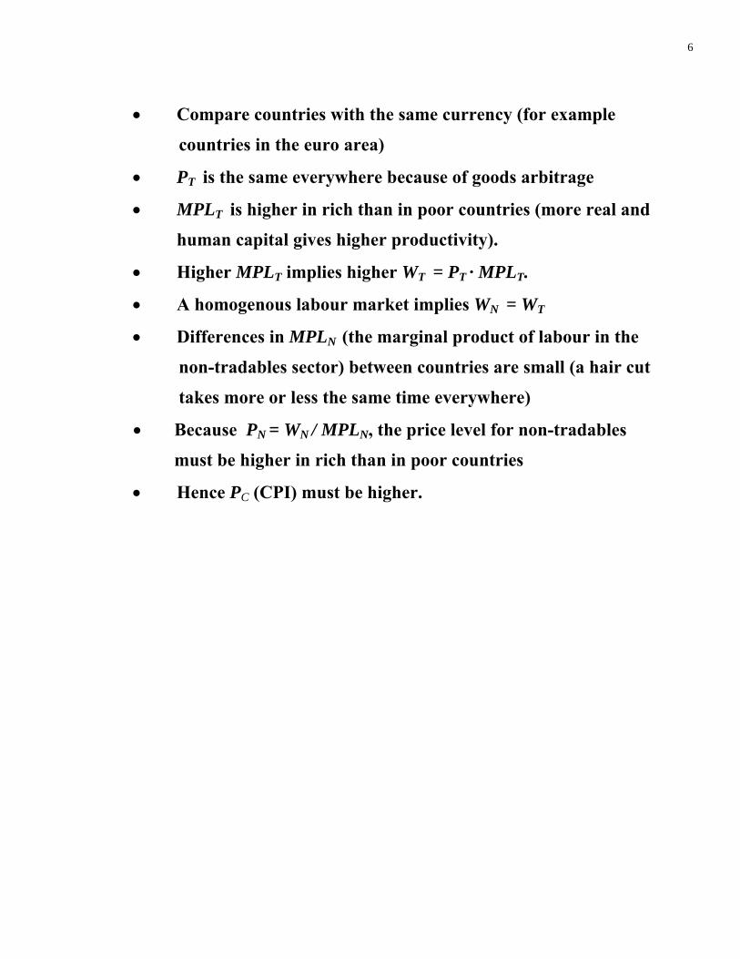
• Compare countries with the same currency (for example

countries in the euro area)

• PT is the same everywhere because of goods arbitrage

• MPLT is higher in rich than in poor countries (more real and

human capital gives higher productivity).

• Higher MPLT implies higher WT = PT · MPLT.

• A homogenous labour market implies WN = WT

• Differences in MPLN (the marginal product of labour in the

non-tradables sector) between countries are small (a hair cut

takes more or less the same time everywhere)

• Because PN = WN / MPLN, the price level for non-tradables

must be higher in rich than in poor countries

• Hence PC (CPI) must be higher.

7

Fig. 15-3: Price Levels and Real Incomes, 2004

Source: Penn World Table, Mark 6.2.

8

• According to the catching-up hypothesis growth is higher in

poor than in rich countries

• The main difference in growth is higher productivity growth

in the tradables sector (manufacturing)

• Poor countries with high growth tend to have higher inflation

that rich: with a common currency (fixed exchange rates),

Estonia and Latvia will have higher inflation than Germany.

9

(1)

(2)

(3)

(4)

(5)

(1 ) (1 ) N N

N N

T T

T T

T T T

T T T

N T

N T

N N N

N N N

C NT T

T N TC

W MPLW MPL

P PEP E P

W P MPLW P MPL

W WW W

P W MPLP W MPL

P PP PP P P Pα α α α

⎧ ⎫⎪⎨ ⎬⎪⎩

∗

Δ Δ−

Δ ΔΔ= +

Δ Δ Δ= +

Δ Δ=

Δ Δ Δ= −

Δ ΔΔ Δ= + − = + −

+

(1 ) (1 )

(1 )

N NT T T

T N T T N

NT

T N

T T

T T

T

T

MPL MPLW P MPLW MPL P MPL MPL

MPLMPLMPL MPL

P PP P

PP

α α α α

α

⎪

⎪⎭

⎧ ⎫ ⎧ ⎫⎪ ⎪ ⎪ ⎪⎨ ⎬ ⎨ ⎬⎪ ⎪ ⎪ ⎪⎩ ⎭ ⎩ ⎭

⎧ ⎫⎪ ⎪⎨ ⎬⎪ ⎪⎩ ⎭

Δ ΔΔ Δ Δ− −

ΔΔ −

=

Δ Δ= + − = + − =

Δ= + −

Higher inflation in poor than in rich countries

10

Arithmetical illustration of Balassa-Samuelson effect

T

T

PP

Δ = 0

N

N

MPLMPL

Δ = 1 %

α = 0,5 Estonia

T

T

MPLMPL

Δ = 8 %

(1 )C TTC

P PP Pα αΔ Δ

= + − NT

T N

MPLMPLMPL MPL

⎧ ⎫⎪ ⎪⎨ ⎬⎪ ⎪⎩ ⎭

ΔΔ − = 0 + 0,5 (8-1) = 3,5 %

Germany

T

T

MPLMPL

Δ = 4 %

(1 )C T

TC

P PP Pα αΔ Δ

= + − NT

T N

MPLMPLMPL MPL

⎧ ⎫⎪ ⎪⎨ ⎬⎪ ⎪⎩ ⎭

ΔΔ− = 0 + 0,5 (4-1) = 1,5 %

• Inflation should be about 2 percentage points higher in Estonia than in Germany because of higher growth.

11

The monetary approach to the exchange rate

€

$

/

/ ( , )

/ ( , )

EUS

SUS US US

SE E E

E P P

P M L R Y

P M L R Y

=

=

=

The fundamental exchange rate equation

$€ / / ( , ) / ( , )]) [ (S S

EUSE EUS USM ME P P Y L R YL R== i

An increase in money supply in the US relative to Europe

/ ( )S SEUSM M ↑ causes a nominal depreciation of the dollar (E↑).

12

The Fisher effect

(1) €$ ( ) / eR R E E E= + − Interest rate parity

(2)

e e eEUS

E EE π π− = − Relative PPP

Substitution of (2) in (1):

€$ e eEUSR R π π− = −

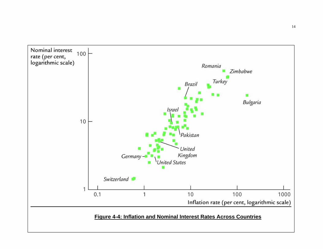
The Fisher effect: a 1 percentage point rise in inflation in

one country causes a 1 percentage point increase in the

nominal interest rate.

13

Figure 4-3: Inflation and Nominal Interest Rates Over Time

14

Figure 4-4: Inflation and Nominal Interest Rates Across Countries

15

Real and nominal exchange rates

q = EPE/PUS

• With a flexible nominal exchange rate, the real exchange

rate can change both because the nominal exchange rate

(E) and the relative price in national currencies (PE/PUS)

change.

• In a currency union (or with a fixed nominal exchange)

rate the real exchange rate can change only through a

change in the relative price in national currencies

• If output/employment in the long run increase in the US

relative to Europe, the relative price of American goods

must fall if these are to be sold, i.e. there must be a real

depreciation for the US.

The real exchange rate equation can be rearranged:

E = q i PUS/PE

The nominal exchange rate (E) can change either because

the relative price level in national currencies between the

countries (PE/PUS) changes or because the real exchange rate

(q) changes.

16

Copyright © 2006 Pearson Addison-Wesley. All rights reserved. 15-38

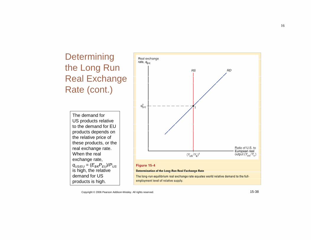
Determining the Long Run Real Exchange Rate (cont.)

The demand forUS products relativeto the demand for EUproducts depends onthe relative price ofthese products, or thereal exchange rate.When the real exchange rate, qUS/EU = (E$/€PEU)/PUSis high, the relative demand for US products is high.

17

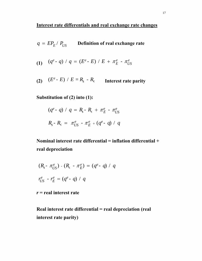
Interest rate differentials and real exchange rate changes

EEPP= / E USq EP P= Definition of real exchange rate

(1) ( - ) / ( - ) / - e e e eE USq q q E E E π π= +

(2) €$( - ) / = - eE E E R R Interest rate parity

Substitution of (2) into (1):

€$

€$

( - ) / - -

- - ( - ) /

e e eE US

e e eEUS

q q q R R

R R q q q

π π

π π +

= +

=

Nominal interest rate differential = inflation differential +

real depreciation

€$ -

( - ) ( - ) ( - ) /

- ( - ) /

e e eEUS

e e eEUS

R R q q q

r r q q q

π π =

=

r = real interest rate

Real interest rate differential = real depreciation (real

interest rate parity)

18

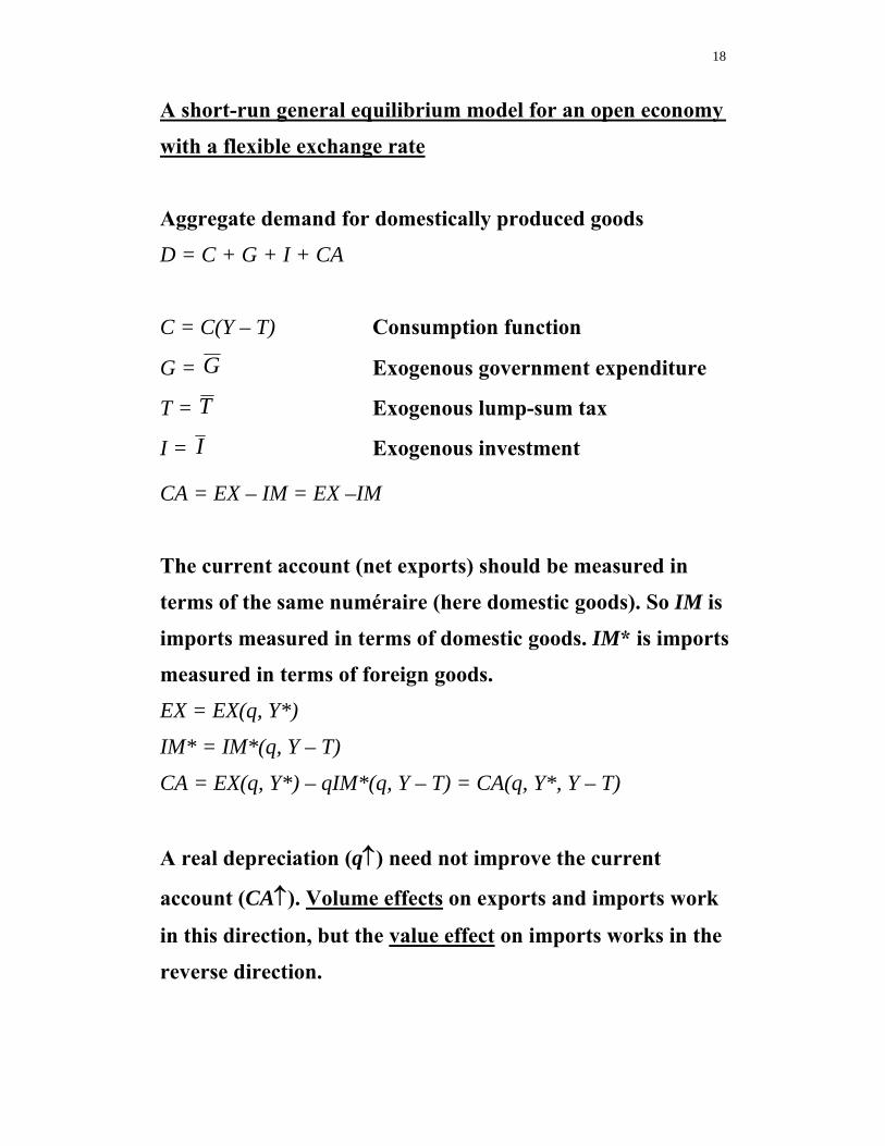
A short-run general equilibrium model for an open economy

with a flexible exchange rate

Aggregate demand for domestically produced goods

D = C + G + I + CA

C = C(Y – T) Consumption function

G = G Exogenous government expenditure

T = T Exogenous lump-sum tax

I = I Exogenous investment

CA = EX – IM = EX –IM

The current account (net exports) should be measured in

terms of the same numéraire (here domestic goods). So IM is

imports measured in terms of domestic goods. IM* is imports

measured in terms of foreign goods.

EX = EX(q, Y*)

IM* = IM*(q, Y – T)

CA = EX(q, Y*) – qIM*(q, Y – T) = CA(q, Y*, Y – T)

A real depreciation (q↑) need not improve the current

account (CA↑). Volume effects on exports and imports work

in this direction, but the value effect on imports works in the

reverse direction.

19

Marshall-Lerner condition

A real depreciation will increase net exports if the Marshall-

Lerner condition holds.

The price elasticity of exports + the price elasticity of imports > 1

Then the volume effects dominate the value effect for imports.

All elasticities are defined to be positive.

20

Mathematical derivation

( , *, ) ( , *) *( , )CA q Y Y T EX q Y qIM q Y T− = − −

Rule of differentiation for a product

( ) ( )

( ) ( ) ( ) ( )x xd v x u x

v x u x u x v xdx

⎡ ⎤⎢ ⎥⎣ ⎦ = +

A real depreciation (q↑) improves the current account (CA↑)

if dCA/dq = CAq > 0.

* *q qdCA EX qIM IMdq = − −

Multiply the equation by q/EX. 2 * * q qq IMqEXq qIMdCA

EX EX EX EXdq = − −i

Assume that CA = 0 initially, so that EX = qIM*=IM.

*

* 1*

> 0 > 1*

q

q

q

q

qIMqEXq dCAEX EXdq IM

qIMqEXdCAEXdq IM

= − −

⇔ −

i

qqEX q EXEX EX q η∂= = =∂i price elasticity of exports

* * * *qqIM q IM

qIM IM η−∂= − = ∗ =∂i price elasticity of imports

All price elasticities have been defined so that they are positive.

1 / 0.dCA dqη η+ ∗ > ⇔ >∵

21


Trade Elasticities

• Insert Table 16AII here

23


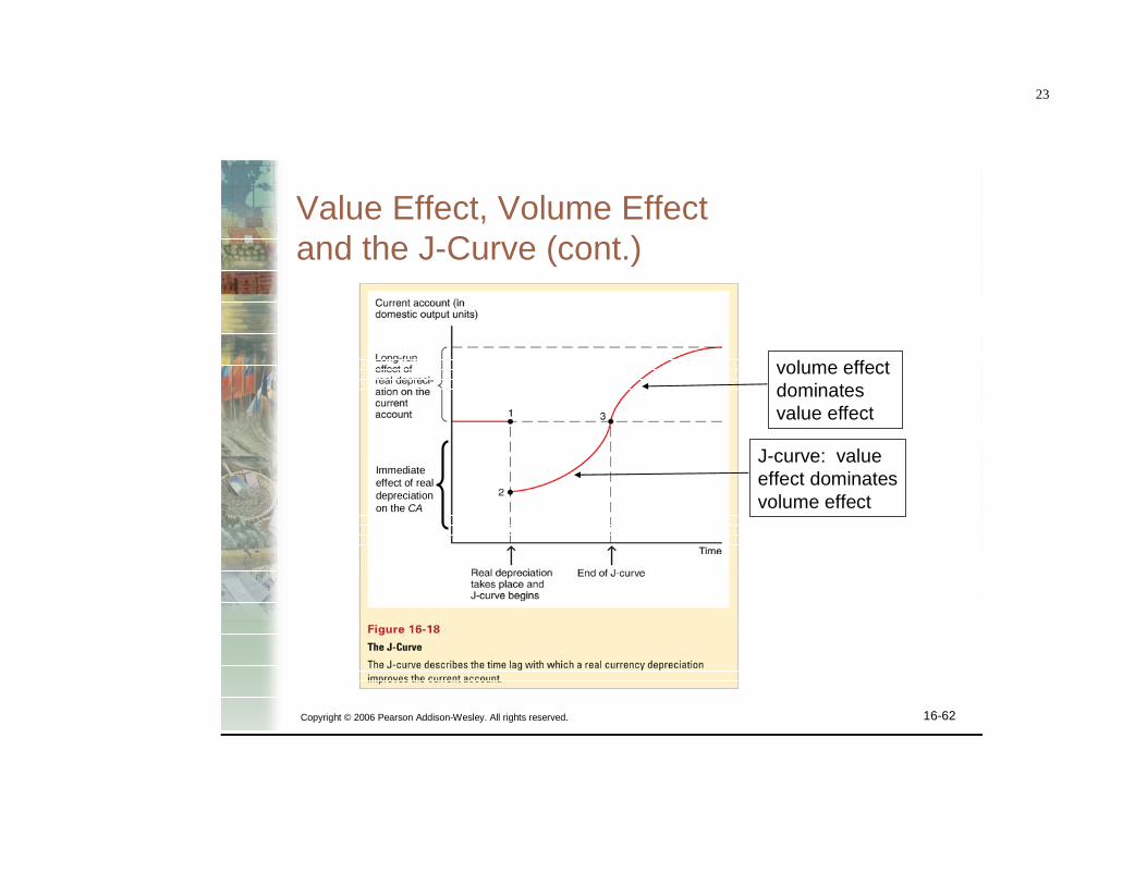
Value Effect, Volume Effect and the J-Curve (cont.)

J-curve: valueeffect dominatesvolume effect

volume effect dominatesvalue effect

Immediateeffect of real depreciationon the CA

24

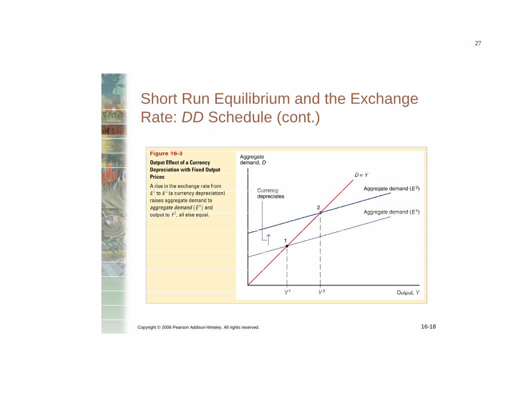
D = C(Y – T) + G + I + CA(EP*/P, Y*, Y – T)

D = D(EP*/P, Y – T, G, I, Y*)

EP*/P↑ ⇒ D↑

(Y – T)↑ ⇒ D↑

G↑ ⇒ D↑

I↑ ⇒ D↑

Y*↑ ⇒ D↑

25


26


Short Run Equilibrium for Aggregate Demand and Output (cont.)

Aggregatedemand isgreater thanproduction: firms increaseoutput

Output is greaterthan aggregate demand: firmsdecrease output

27


Short Run Equilibrium and the Exchange Rate: DD Schedule (cont.)

28


Short Run Equilibrium and the Exchange Rate: DDSchedule (cont.)

29


Shifting the DDCurve (cont.)

30

Changes shifting the DD-curve to the right

1. An increase in government expenditure (G↑)

2. A reduction in the tax (T↓)

3. An increase in investment (I↑)

4. A reduction in the domestic price level (P↓)

5. An increase in the foreign price level (P*↑)

6. An increase in foreign income (Y*↑)

7. A reduction in the savings rate (s↓)

8. A shift in expenditure from foreign to domestic goods

(increased relative demand for domestic goods)

31

Equilibrium in asset markets

1. Foreign currency market (interest rate parity)

R = R* + (Ee – E)/E

2. Money market

Ms/P = L(R, Y)

32


Short Run Equilibrium for Assets (cont.)

33


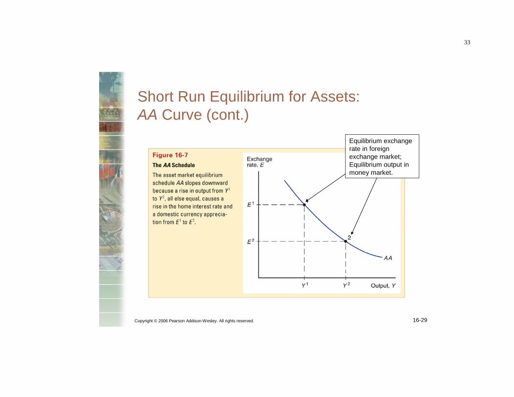
Short Run Equilibrium for Assets: AA Curve (cont.)

Equilibrium exchange rate in foreign exchange market;Equilibrium output in money market.

34

Factors shifting the AA-curve upwards

1. An increase in money supply (Ms↑)

2. A reduction in the price level (P↓)

3. An expected future depreciation (Ee↑ )

4. A higher foreign interest rate (R*↓)

5. A reduction in domestic money demand

35

E

M/P

R, R*+(Ee – E)/E

E

Y

A

A

AN INCREASE IN MONEY SUPPLY, A REDUCTION OF THE PRICE LEVEL

Mo/P

M1/P

36

E

M/P

R, R*+(Ee – E)/E

E

Y

A

A

AN EXPECTED DEPRECIATION, AN INCREASE IN THE FOREIGN INTEREST RATE

37


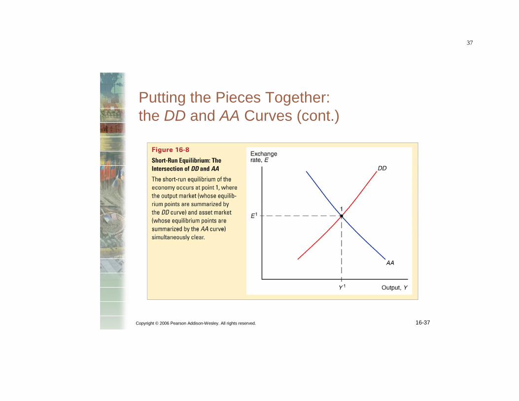
Putting the Pieces Together: the DD and AA Curves (cont.)

38


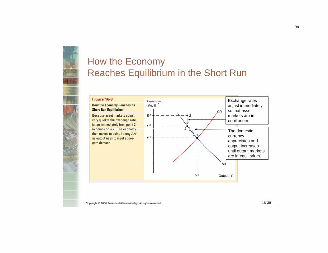
The domestic currency appreciates and output increases until output markets are in equilibrium.

Exchange rates adjust immediately so that asset markets are in equilibrium.

How the Economy Reaches Equilibrium in the Short Run

39


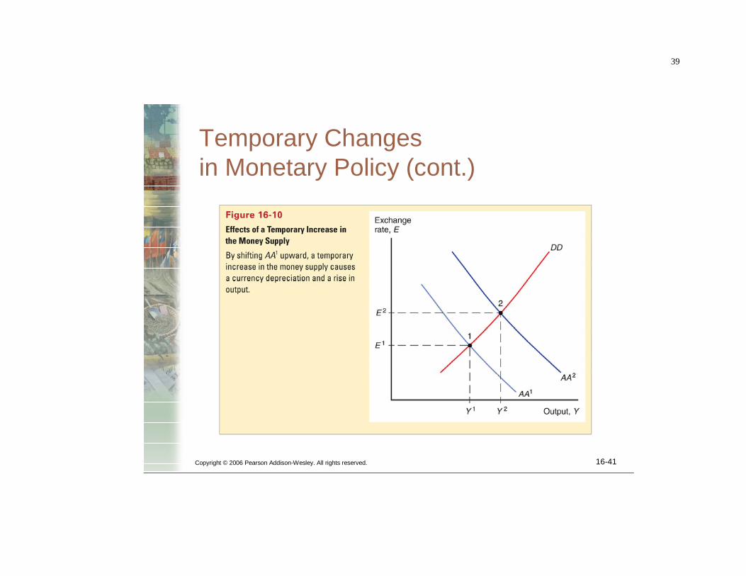
Temporary Changes in Monetary Policy (cont.)

40


Temporary Changes in Fiscal Policy (cont.)

41

16-45

Policies to Maintain Full Employment (cont.)

Temporary fiscal policy could reverse the fall in aggregate demand and output

Temporary fall in world demand for domestic products reduces output below its normal level

Temporary monetaryexpansion could depreciate the domestic currency

42

Problems with stabilisation policy

• Policies can easily become too expansionary on average

(”inflation bias”)

• It is difficult ex ante to identify disturbances and how

strong they are

• An expansionary fiscal policy can cause permanent

budget deficits

• ”Decision lags”

43


Effects of Permanent Changes in Monetary Policy in the Short Run

A permanent increase in the money supply decreases interest rates and causes people to expect a future depreciation, leading to a large actual depreciation

44


Effects of Permanent Changes in Monetary Policy in the Long Run (cont.)

In the long run, output returns to its normal level, and we also see overshooting: E1 < E3 < E2

Higher prices make domestic products more expensive relative to foreign goods: reduction in aggregate demand

Higher prices reducereal money supply,Increasing interest rates, leading to adomestic currency appreciation

45


Effects of Permanent Changes in Fiscal Policy (cont.)

An increase ingovernment purchases raisesaggregate demand

Temporary fiscalexpansion outcome

When the increase of government purchases is permanent, the domestic currency is expected to appreciate, and does appreciate.

46

Why has a permanent fiscal policy no output effects?

1. In the long run we have Y = Yf och R = R* (output and

interest rate at their equilibrium levels). Because P =

Ms/L(Yf, R*,) P must be unchanged in the long run.

2. In the short run Ms/P is given. Assume that Y↑. Then R↑.

From interest rate parity we then have (Ee – E)↑.

A nominal exchange rate depreciation is expected.

3. But an expected nominal depreciation must also imply an

expected real depreciation as P is given in the long run.

This cannot be true because Y must then increase even

more in the long run than in the short run and can then

never return to its equilibrium level Yf.

4. But everything will fit together if Y never changes, so

that Y = Yf even in the short run.

47

The mathematics of a permanent fiscal expansion

sM

P = L(Y, R) (1)

R = R* + (Ee – E)/E (2)

Y = D(EP*/P, Y-T, I, G, Y*) (3)

If↑ ⇒ E = Ee ↓ so that Y remains constant according to

equation (3), equations (1) and (2) are also fulfilled.

48

Further aspects on exchange rates

• The current account and the exchange rate

• Investors might start to question US ability to service

debt (cumulated current account deficits)

• Capital inflows to the US could stop and capital flows

could even be reversed: unless the current account

deficits are offset by capital inflows there will be an

excess supply of dollars and the dollar must depreciate.

• But US assets abroad are mostly denominated in

foreign currency, whereas debt is in dollars, so a

depreciation of the dollar will reduce US net debt to the

rest of the world

• Hence no risk that the value effects of a dollar

depreciation would lead to a financial crisis because net

foreign debt would increase (as has happened in many

emerging economies

Lecture 5: Intermediate macroeconomics, autumn 2008perseus.iies.su.se/~calmf/Ekonomisk...

Documents

Transcript of Lecture 5: Intermediate macroeconomics, autumn 2008perseus.iies.su.se/~calmf/Ekonomisk...