Lecture 3Instruction Set Architecture

Computer Architectures 521480S

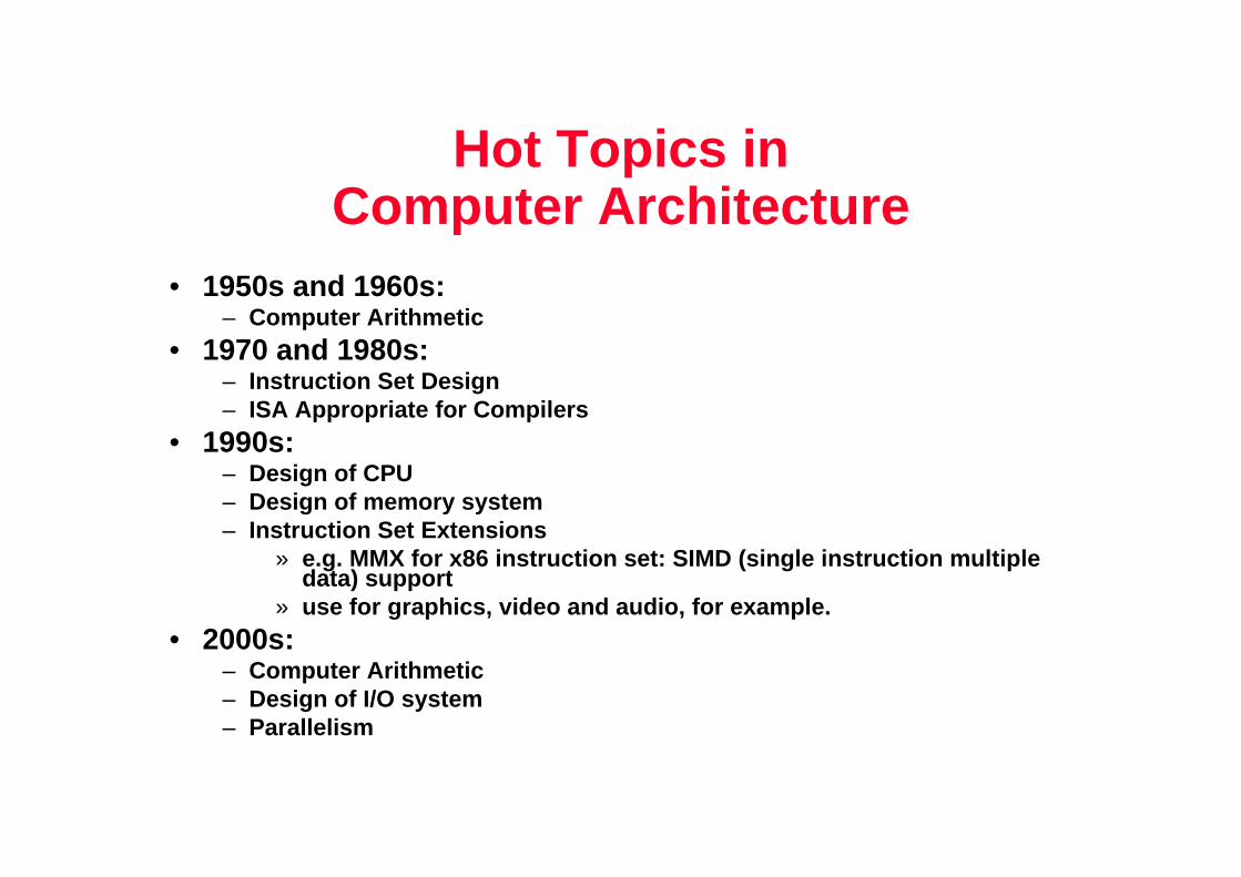
Hot Topics in Computer Architecture

• 1950s and 1960s:– Computer Arithmetic

• 1970 and 1980s: – Instruction Set Design– ISA Appropriate for Compilers

• 1990s: – Design of CPU– Design of memory system– Instruction Set Extensions

» e.g. MMX for x86 instruction set: SIMD (single inst ruction multiple data) support

» use for graphics, video and audio, for example.• 2000s:

– Computer Arithmetic – Design of I/O system– Parallelism

Instruction Set Architecture

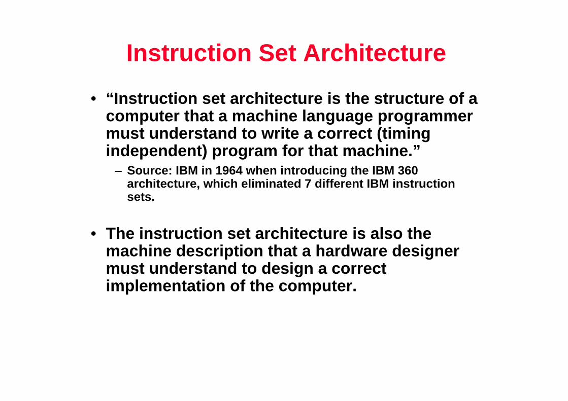
• “Instruction set architecture is the structure of a computer that a machine language programmer must understand to write a correct (timing independent) program for that machine.”

– Source: IBM in 1964 when introducing the IBM 360 architecture, which eliminated 7 different IBM instr uction sets.

• The instruction set architecture is also the machine description that a hardware designer must understand to design a correct implementation of the computer.

RHK.S96 4

Interface Design

A good interface:

• Lasts through many implementations (portability,compatibility)

• Is used in many different ways (generality)

• Provides convenient functionality to higher levels

• Permits an efficient implementation at lower levels

Instruction Set Architecture

High level language code : C, C++, Java, Fortan ,

• The instruction set architecture serves as the interface between software and hardware.

• It provides the mechanism by which the software tells the hardware what should be done.

Assembly language code: architecture specific state ments

Machine language code: architecture specific bit pat terns

compiler

assembler

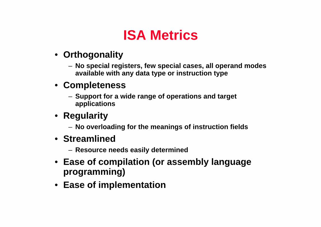
ISA Metrics• Orthogonality

– No special registers, few special cases, all operan d modes available with any data type or instruction type

• Completeness– Support for a wide range of operations and target

applications

• Regularity– No overloading for the meanings of instruction fiel ds

• Streamlined– Resource needs easily determined

• Ease of compilation (or assembly language programming)

• Ease of implementation

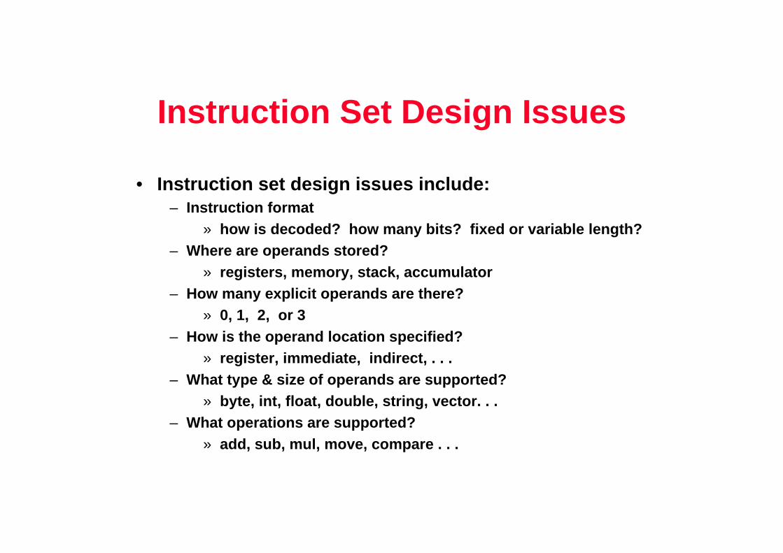
Instruction Set Design Issues

• Instruction set design issues include:– Instruction format

» how is decoded? how many bits? fixed or variable length?– Where are operands stored?

» registers, memory, stack, accumulator– How many explicit operands are there?

» 0, 1, 2, or 3 – How is the operand location specified?

» register, immediate, indirect, . . . – What type & size of operands are supported?

» byte, int, float, double, string, vector. . .– What operations are supported?

» add, sub, mul, move, compare . . .

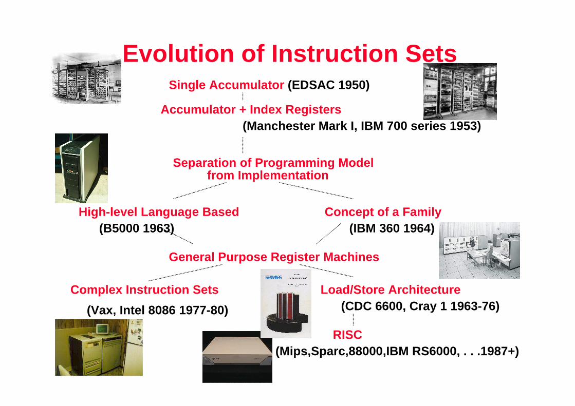
Evolution of Instruction SetsSingle Accumulator (EDSAC 1950)

Accumulator + Index Registers(Manchester Mark I, IBM 700 series 1953)

Separation of Programming Modelfrom Implementation

High-level Language Based Concept of a Family(B5000 1963) (IBM 360 1964)

General Purpose Register Machines

Complex Instruction Sets Load/Store Architecture

RISC

(Vax, Intel 8086 1977-80) (CDC 6600, Cray 1 1963-76)

(Mips,Sparc,88000,IBM RS6000, . . .1987+)

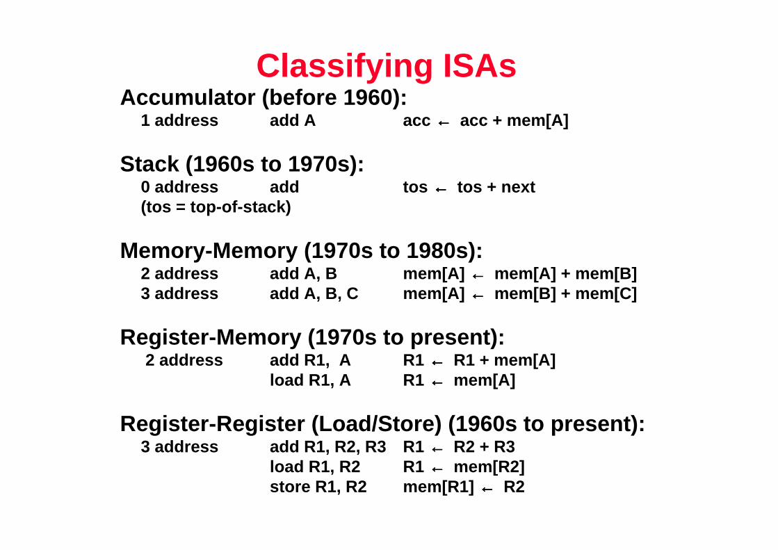
Classifying ISAsAccumulator (before 1960):

1 address add A acc ←←←← acc + mem[A]

Stack (1960s to 1970s):0 address add tos ←←←← tos + next(tos = top-of-stack)

Memory-Memory (1970s to 1980s):2 address add A, B mem[A] ←←←← mem[A] + mem[B]3 address add A, B, C mem[A] ←←←← mem[B] + mem[C]

Register-Memory (1970s to present):2 address add R1, A R1 ←←←← R1 + mem[A]

load R1, A R1 ←←←← mem[A]

Register-Register (Load/Store) (1960s to present):3 address add R1, R2, R3 R1 ←←←← R2 + R3

load R1, R2 R1 ←←←← mem[R2]store R1, R2 mem[R1] ←←←← R2

RHK.S96 10

Comparison of ISA Classes

• Code Sequence for C = A+B

Stack Accumulator Register(register-Mem)

Register(load/store)

Push A Load A Load R1, A Load R1, A

Push B Add B Add R1, B Load R2, B

Add Store C Store C, R1 Add R3, R1, R2

Pop C Store C, R3

• Code density (memory efficiency)?Instruction access? Data access?

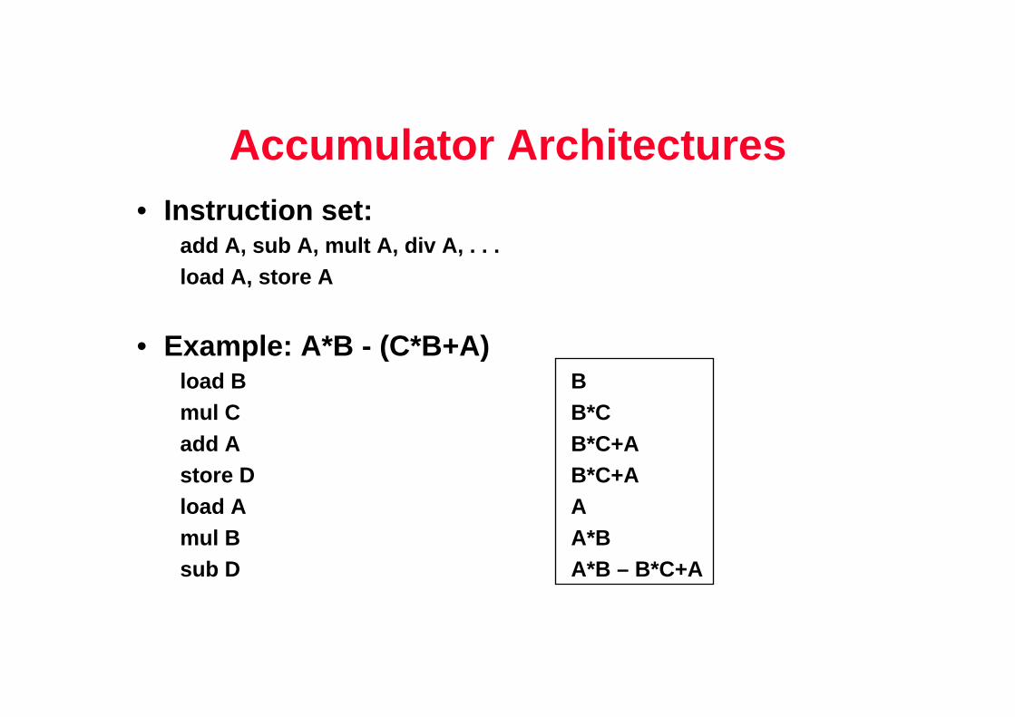
Accumulator Architectures• Instruction set:

add A, sub A, mult A, div A, . . .load A, store A

• Example: A*B - (C*B+A)load B Bmul C B*Cadd A B*C+Astore D B*C+Aload A Amul B A*Bsub D A*B – B*C+A

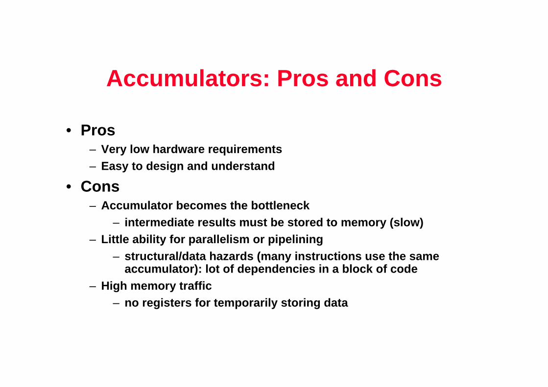
Accumulators: Pros and Cons

• Pros– Very low hardware requirements– Easy to design and understand

• Cons– Accumulator becomes the bottleneck

– intermediate results must be stored to memory (slow )– Little ability for parallelism or pipelining

– structural/data hazards (many instructions use the same accumulator): lot of dependencies in a block of cod e

– High memory traffic– no registers for temporarily storing data

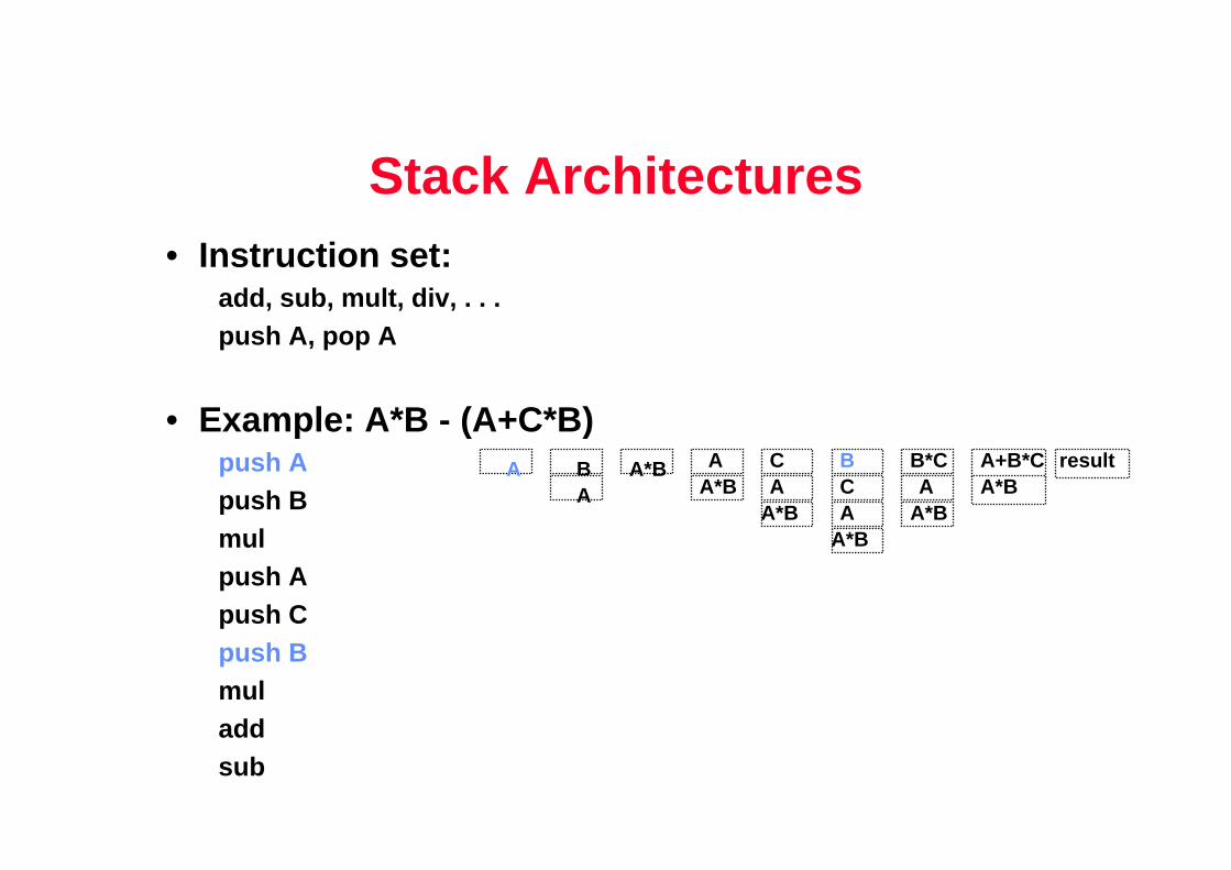
Stack Architectures• Instruction set:

add, sub, mult, div, . . .push A, pop A

• Example: A*B - (A+C*B)push Apush Bmulpush Apush Cpush Bmuladdsub

A BA

A*BA*B

A*BA*B

AAC

A*BA A*B

A C B B*C A+B*C result

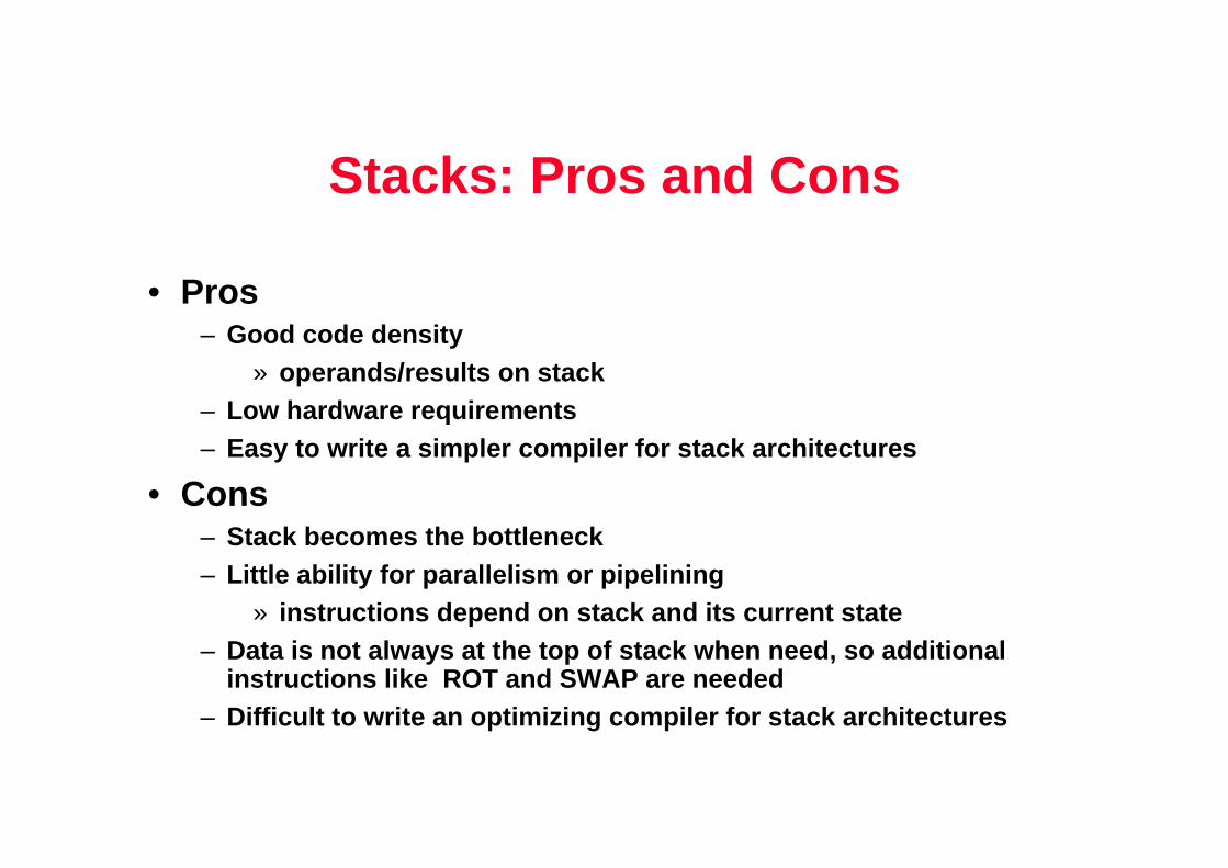
Stacks: Pros and Cons

• Pros– Good code density

» operands/results on stack– Low hardware requirements– Easy to write a simpler compiler for stack architec tures

• Cons– Stack becomes the bottleneck– Little ability for parallelism or pipelining

» instructions depend on stack and its current state– Data is not always at the top of stack when need, s o additional

instructions like ROT and SWAP are needed– Difficult to write an optimizing compiler for stack architectures

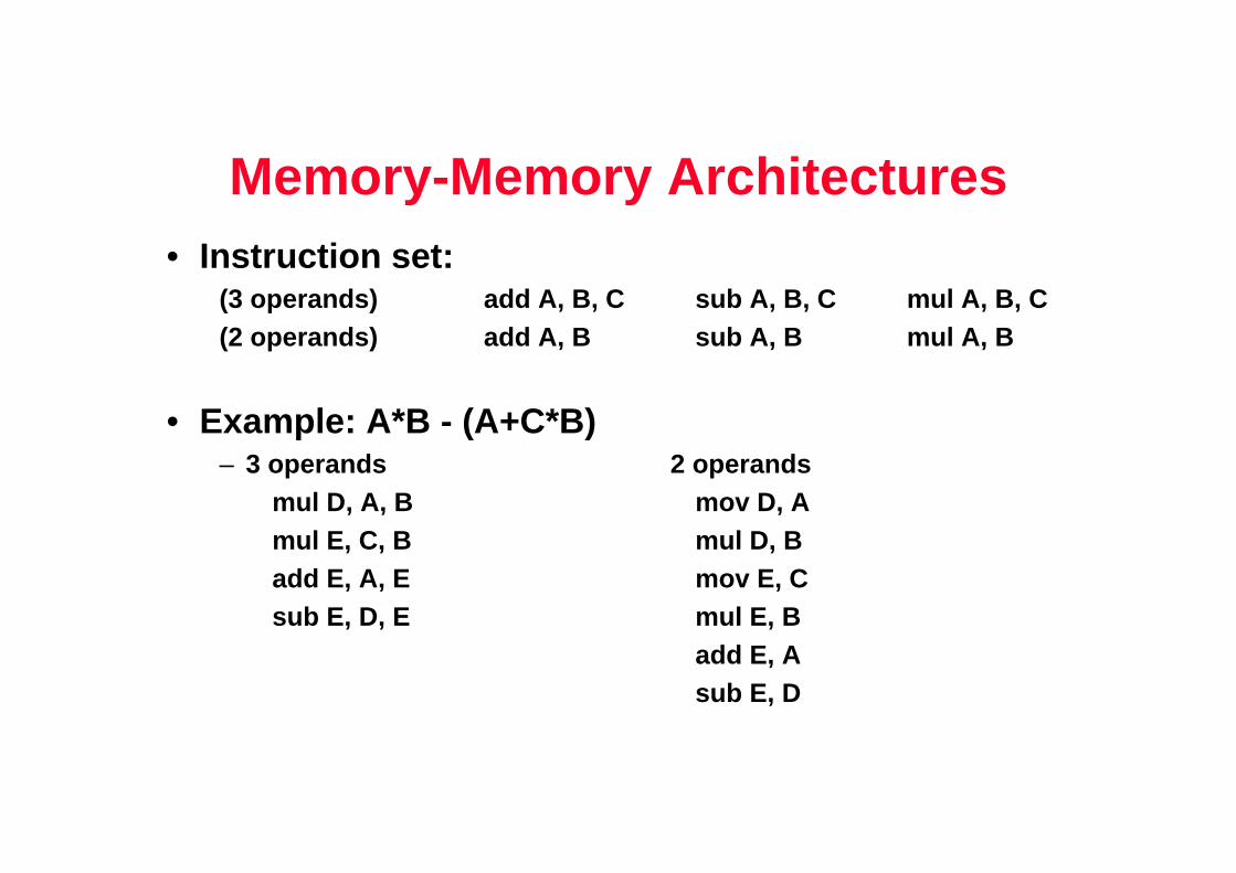
Memory-Memory Architectures• Instruction set:

(3 operands) add A, B, C sub A, B, C mul A, B, C(2 operands) add A, B sub A, B mul A, B

• Example: A*B - (A+C*B)– 3 operands 2 operands

mul D, A, B mov D, Amul E, C, B mul D, Badd E, A, E mov E, Csub E, D, E mul E, B

add E, Asub E, D

Memory-Memory:Pros and Cons

• Pros– Requires fewer instructions (especially if 3 operan ds)

– most compact– Easy to write compilers for (especially if 3 operan ds)

• Cons– Very high memory traffic (especially if 3 operands)– Variable instruction size

– complex instruction decoding

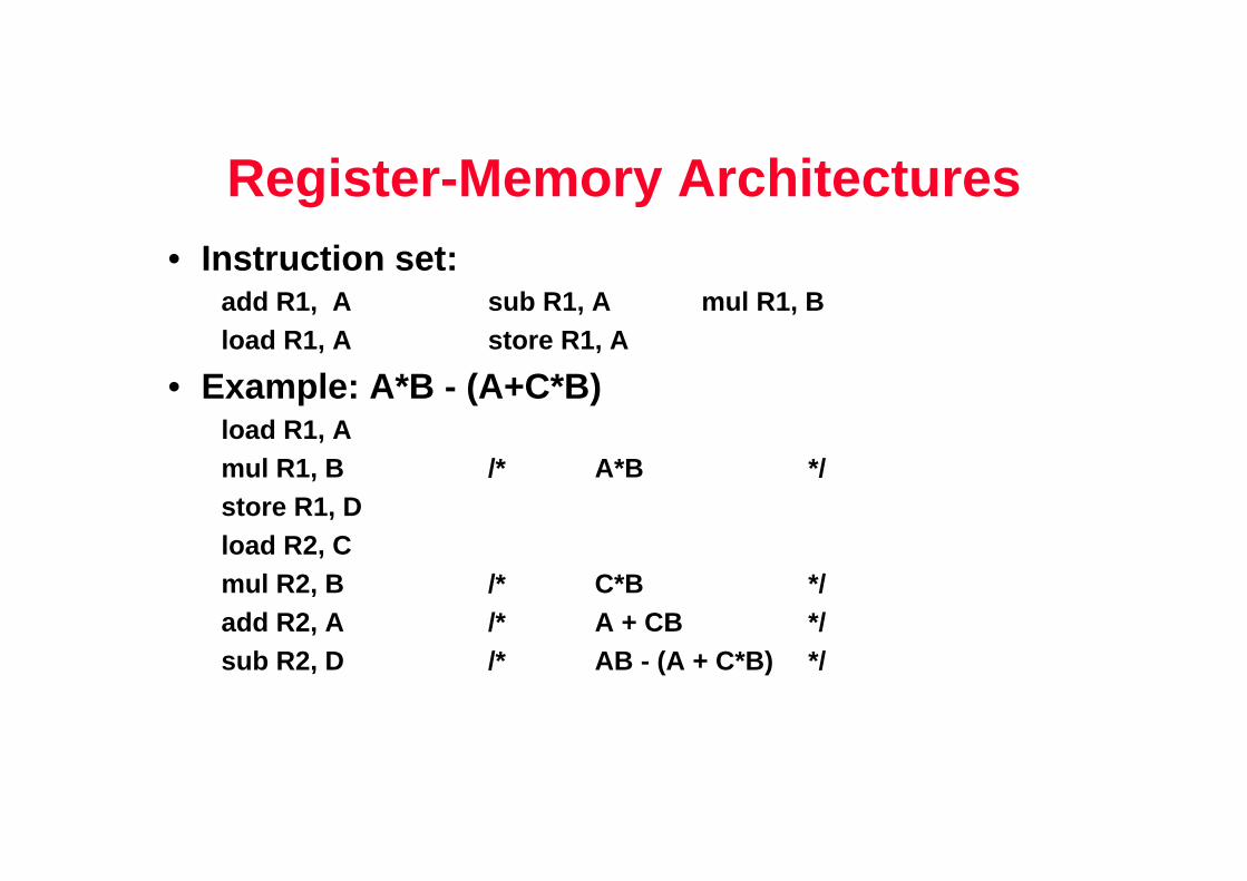
Register-Memory Architectures• Instruction set:

add R1, A sub R1, A mul R1, Bload R1, A store R1, A

• Example: A*B - (A+C*B)load R1, Amul R1, B /* A*B */store R1, Dload R2, Cmul R2, B /* C*B */add R2, A /* A + CB */sub R2, D /* AB - (A + C*B) */

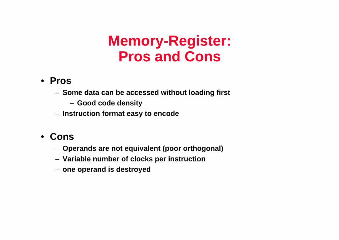
Memory-Register: Pros and Cons

• Pros– Some data can be accessed without loading first

– Good code density– Instruction format easy to encode

• Cons– Operands are not equivalent (poor orthogonal)– Variable number of clocks per instruction– one operand is destroyed

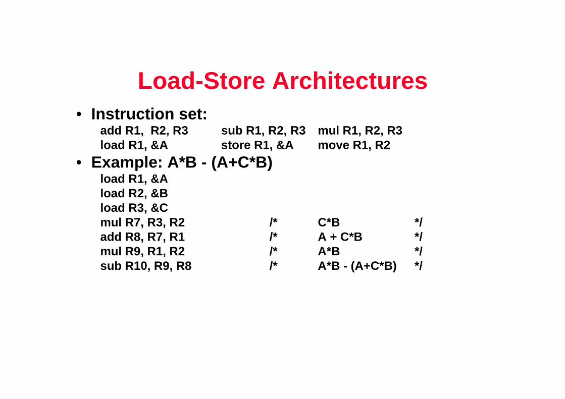
Load-Store Architectures• Instruction set:

add R1, R2, R3 sub R1, R2, R3 mul R1, R2, R3load R1, &A store R1, &A move R1, R2

• Example: A*B - (A+C*B)load R1, &Aload R2, &Bload R3, &Cmul R7, R3, R2 /* C*B */add R8, R7, R1 /* A + C*B */mul R9, R1, R2 /* A*B */sub R10, R9, R8 /* A*B - (A+C*B) */

Load-Store: Pros and Cons

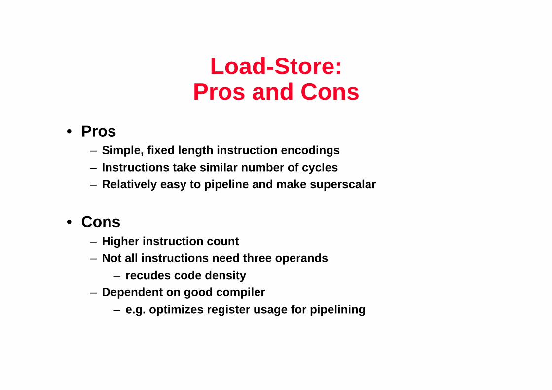
• Pros– Simple, fixed length instruction encodings– Instructions take similar number of cycles– Relatively easy to pipeline and make superscalar

• Cons– Higher instruction count – Not all instructions need three operands

– recudes code density– Dependent on good compiler

– e.g. optimizes register usage for pipelining

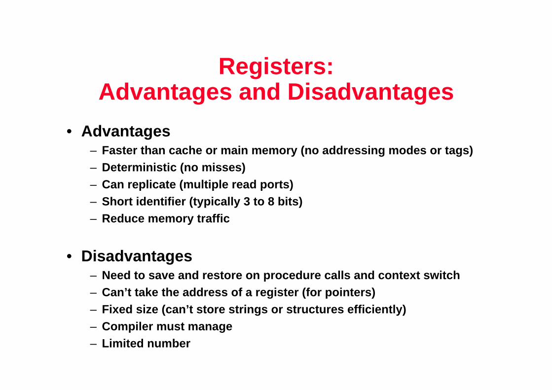
Registers:Advantages and Disadvantages

• Advantages– Faster than cache or main memory (no addressing mod es or tags)– Deterministic (no misses)– Can replicate (multiple read ports)– Short identifier (typically 3 to 8 bits)– Reduce memory traffic

• Disadvantages– Need to save and restore on procedure calls and con text switch– Can’t take the address of a register (for pointers)– Fixed size (can’t store strings or structures effic iently)– Compiler must manage– Limited number

RHK.S96 22

Byte Ordering• Idea

– Bytes in long word numbered 0 to 3– Which is most (least) significant?– Can cause problems when exchanging binary data betw een

machines

• Big Endian: Byte 0 is most, 3 is least– IBM 360/370, Motorola 68K, Sparc.

• Little Endian: Byte 0 is least, 3 is most– Intel x86, VAX

• Alpha– Chip can be configured to operate either way– DEC workstation are little endian– Cray T3E Alpha’s are big endian

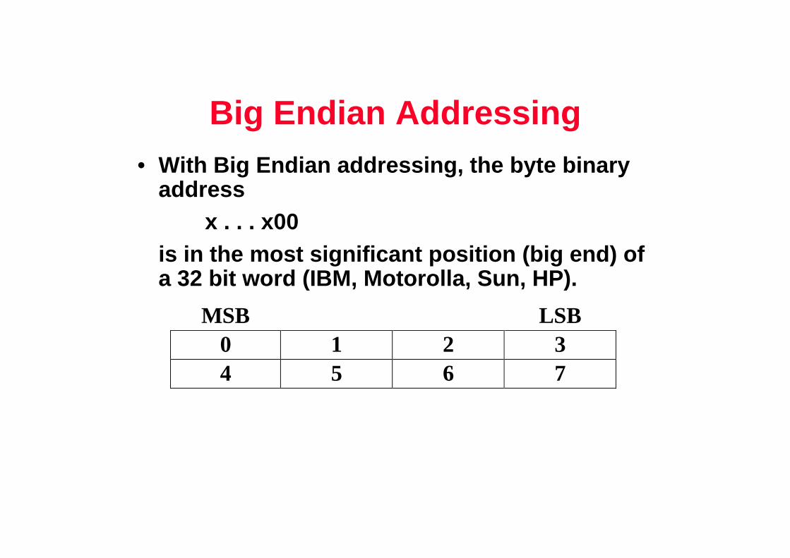
Big Endian Addressing• With Big Endian addressing, the byte binary

address x . . . x00

is in the most significant position (big end) of a 32 bit word (IBM, Motorolla, Sun, HP).

MSB LSB0 1 2 34 5 6 7

Little Endian Addressing• With Little Endian addressing, the byte binary

address x . . . x00

is in the least significant position (little end) of a 32 bit word (DEC, Intel).

MSB LSB3 2 1 07 6 5 4

•Programmers/protocols should be careful when transferring binary data between Big Endian and Little Endian machines

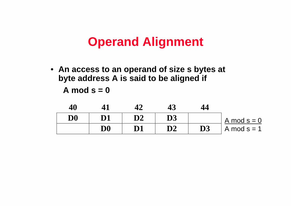
Operand Alignment

• An access to an operand of size s bytes at byte address A is said to be aligned if

A mod s = 0

40 41 42 43 44D0 D1 D2 D3

D0 D1 D2 D3A mod s = 0A mod s = 1

Unrestricted Alignment

• If the architecture does not restrict memory accesses to be aligned then

– Software is simple– Hardware must detect misalignment and make two

memory accesses– Expensive logic to perform detection – Can slow down all references– Sometimes required for backwards compatibility

Restricted Alignment

• If the architecture restricts memory accesses to be aligned then

– Software must guarantee alignment– Hardware detects misalignment access and traps– No extra time is spent when data is aligned

• Since we want to make the common case fast, having restricted alignment is often a better choice, unless compatibility is an issue.

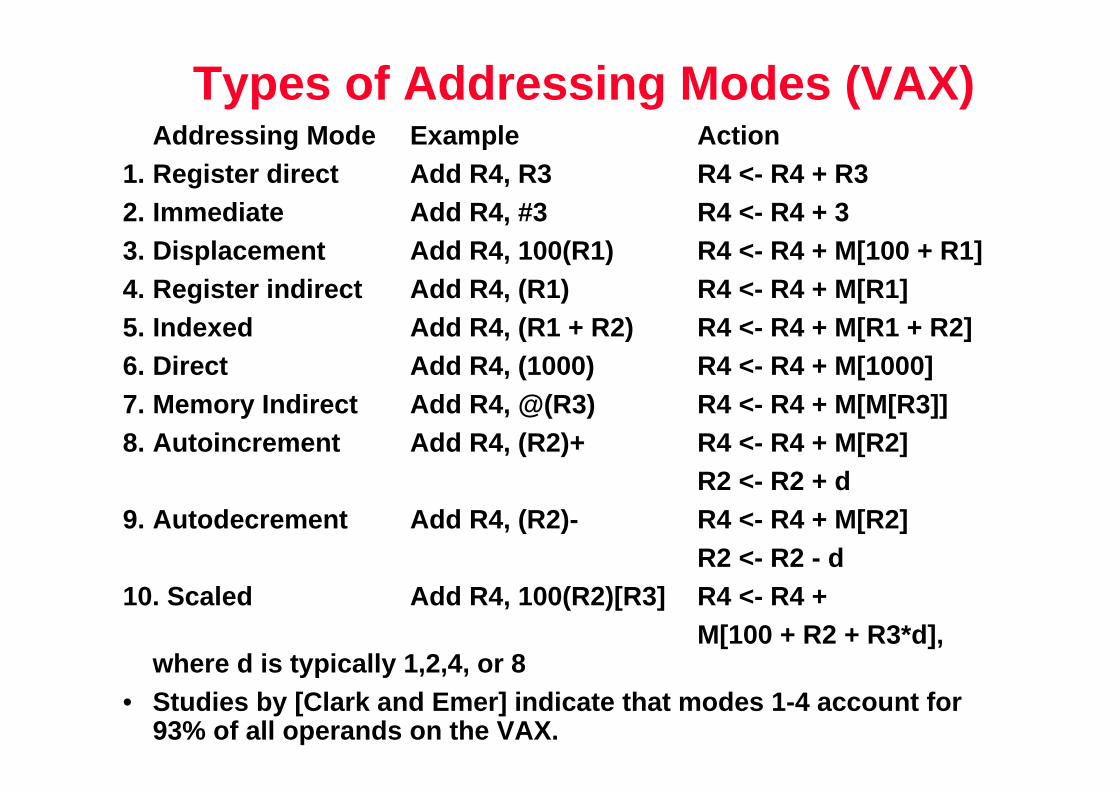
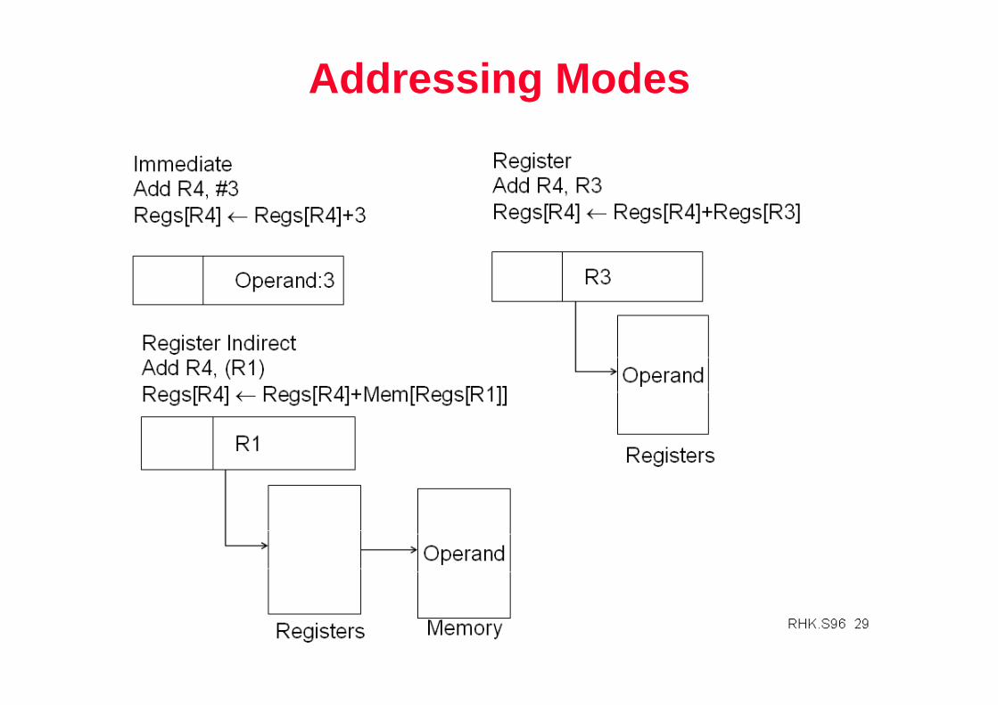
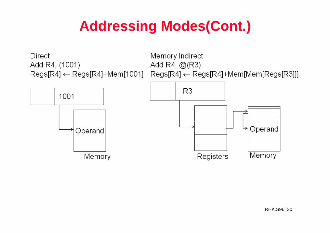
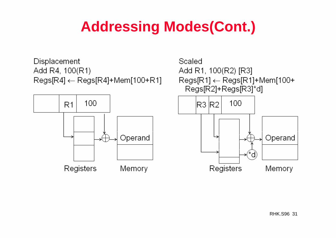
Types of Addressing Modes (VAX)Addressing Mode Example Action

1. Register direct Add R4, R3 R4 <- R4 + R32. Immediate Add R4, #3 R4 <- R4 + 33. Displacement Add R4, 100(R1) R4 <- R4 + M[100 + R1]4. Register indirect Add R4, (R1) R4 <- R4 + M[R1]5. Indexed Add R4, (R1 + R2) R4 <- R4 + M[R1 + R2]6. Direct Add R4, (1000) R4 <- R4 + M[1000]7. Memory Indirect Add R4, @(R3) R4 <- R4 + M[M[R3]]8. Autoincrement Add R4, (R2)+ R4 <- R4 + M[R2]

R2 <- R2 + d 9. Autodecrement Add R4, (R2)- R4 <- R4 + M[R2]

R2 <- R2 - d10. Scaled Add R4, 100(R2)[R3] R4 <- R4 +

M[100 + R2 + R3*d], where d is typically 1,2,4, or 8

• Studies by [Clark and Emer] indicate that modes 1-4 account for 93% of all operands on the VAX.

RHK.S96 29

Addressing Modes

RHK.S96 30

Addressing Modes(Cont.)

RHK.S96 31

Addressing Modes(Cont.)

RHK.S96 32

Types of Operations• Arithmetic and Logical:

– add, subtract, and , or, etc.

• Data transfer:– Load, Store, etc.

• Control– Jump, branch, call, return, trap (= software interr upt), etc.

• Synchronization:– Test & Set

• String:– string move, compare, search.

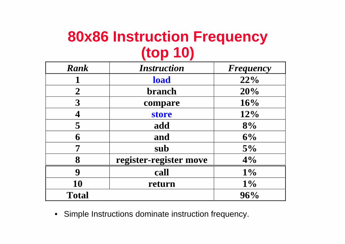
80x86 Instruction Frequency (top 10)

Rank Instruction Frequency 1 load 22% 2 branch 20% 3 compare 16% 4 store 12% 5 add 8% 6 and 6% 7 sub 5% 8 register-register move 4%

9

9 call 1% 10 return 1%

Total 96%

• Simple Instructions dominate instruction frequency.

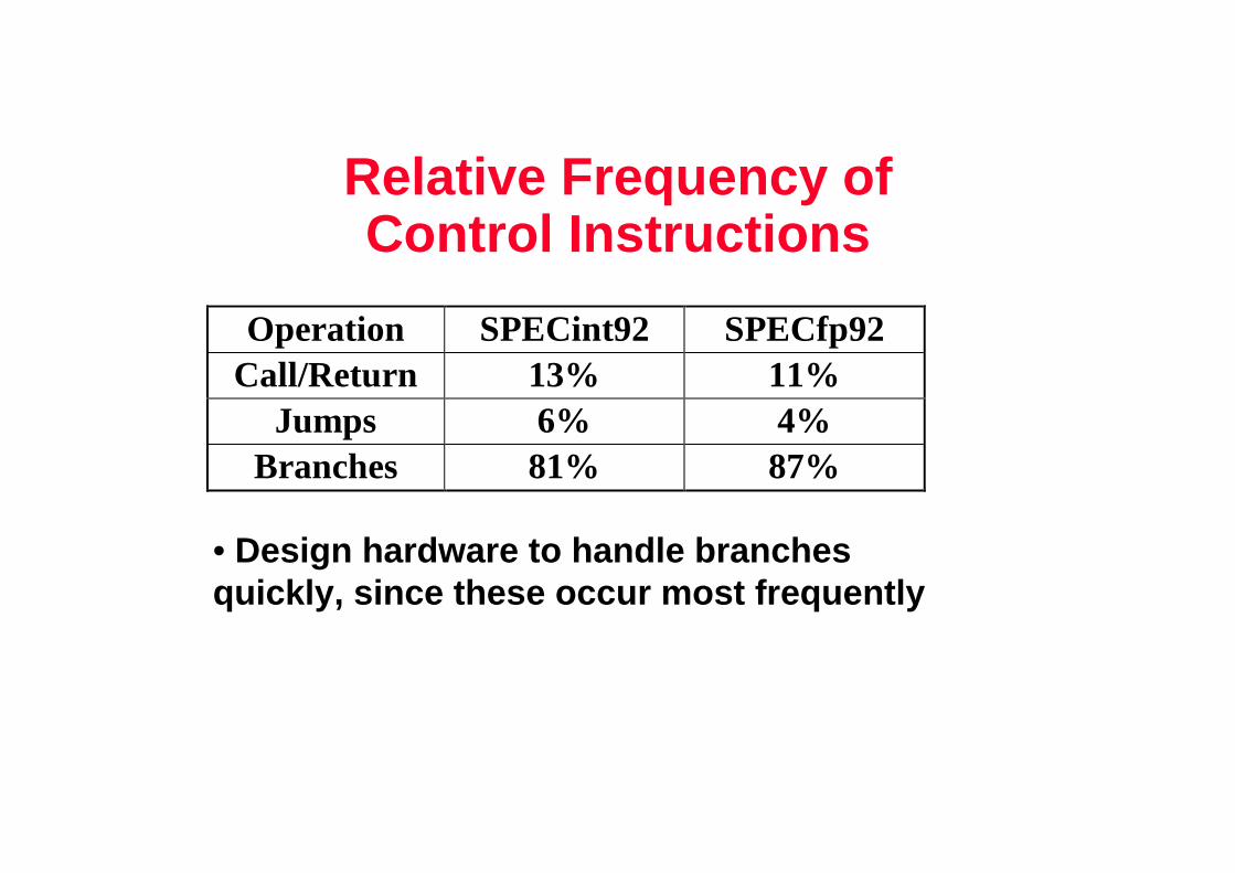
Relative Frequency of Control Instructions

Operation SPECint92 SPECfp92Call/Return 13% 11%

Jumps 6% 4%Branches 81% 87%

• Design hardware to handle branches quickly, since these occur most frequently

RHK.S96 35

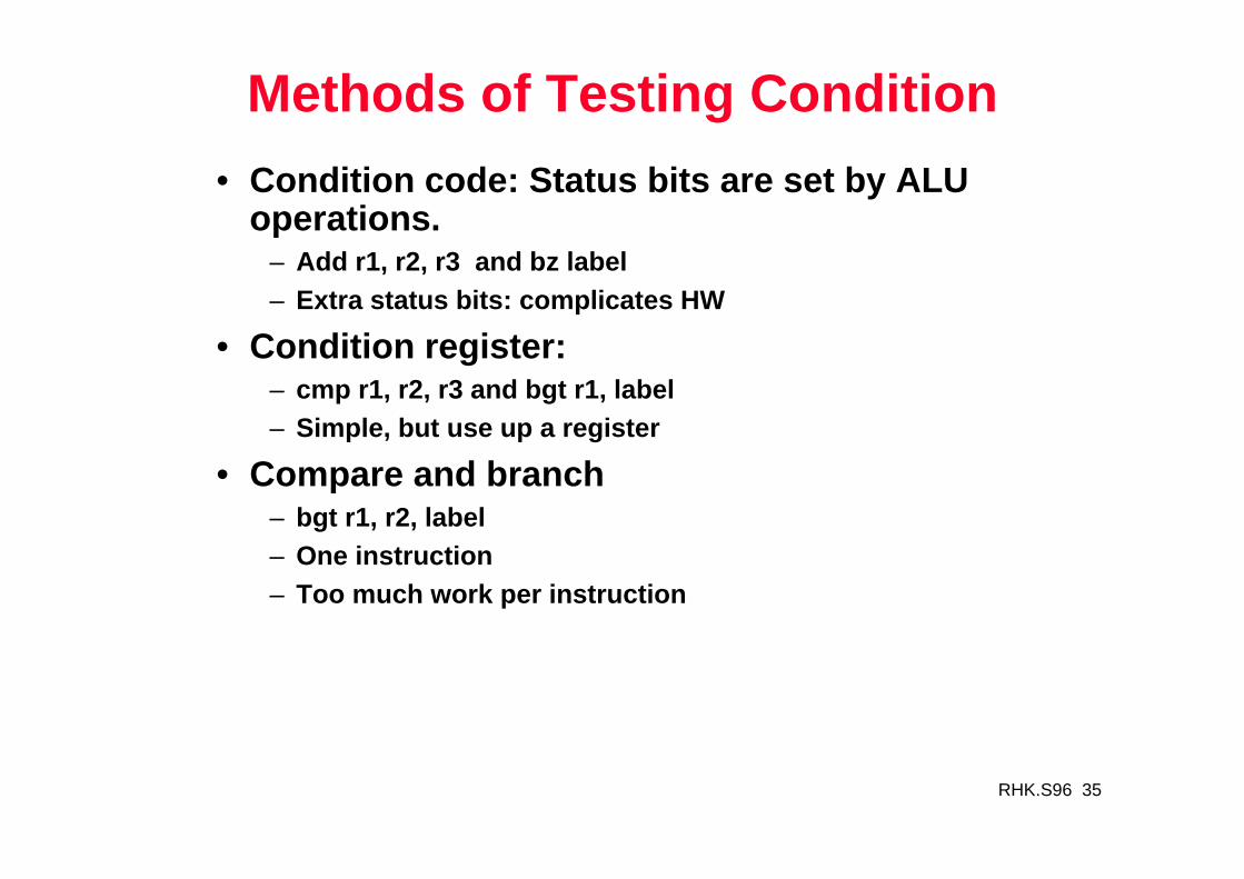
Methods of Testing Condition

• Condition code: Status bits are set by ALU operations.

– Add r1, r2, r3 and bz label– Extra status bits: complicates HW

• Condition register:– cmp r1, r2, r3 and bgt r1, label– Simple, but use up a register

• Compare and branch– bgt r1, r2, label– One instruction– Too much work per instruction

RHK.S96 36

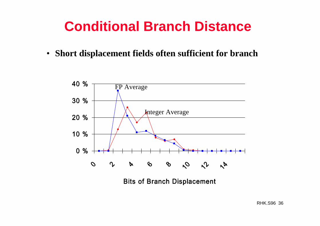
Conditional Branch Distance

• Short displacement fields often sufficient for branch

0 %0 %0 %0 %

10 %10 %10 %10 %

20 %20 %20 %20 %

30 %30 %30 %30 %

40 %40 %40 %40 %

0000 2222 4444 6666 8888 10101010 12121212 14141414

Bits of Branch DisplacementBits of Branch DisplacementBits of Branch DisplacementBits of Branch Displacement

Integer Average

FP Average

RHK.S96 37

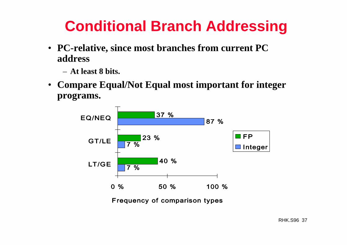
Conditional Branch Addressing• PC-relative, since most branches from current PC

address– At least 8 bits.

• Compare Equal/Not Equal most important for integer programs.

7 %7 %7 %7 %

7 %7 %7 %7 %

87 %87 %87 %87 %

40 %40 %40 %40 %

23 %23 %23 %23 %

37 %37 %37 %37 %

0 %0 %0 %0 % 50 %50 %50 %50 % 100 %100 %100 %100 %

LT/GELT/GELT/GELT/GE

GT/LEGT/LEGT/LEGT/LE

EQ/NEQEQ/NEQEQ/NEQEQ/NEQ

Frequency of comparison typesFrequency of comparison typesFrequency of comparison typesFrequency of comparison types

FPFPFPFPIntegerIntegerIntegerInteger

RHK.S96 38

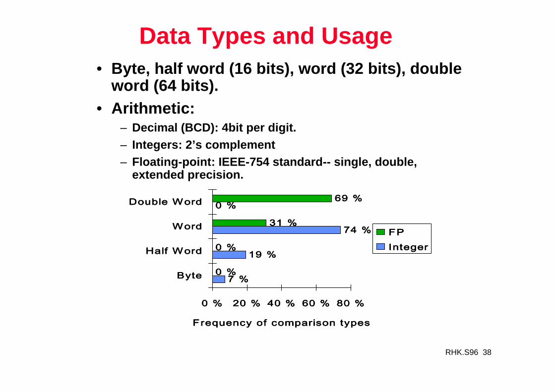
Data Types and Usage• Byte, half word (16 bits), word (32 bits), double

word (64 bits).• Arithmetic:

– Decimal (BCD): 4bit per digit.– Integers: 2’s complement– Floating-point: IEEE-754 standard-- single, double,

extended precision.

7 %7 %7 %7 %

19 %19 %19 %19 %

74 %74 %74 %74 %

0 %0 %0 %0 %

0 %0 %0 %0 %

0 %0 %0 %0 %

31 %31 %31 %31 %

69 %69 %69 %69 %

0 %0 %0 %0 % 20 %20 %20 %20 % 40 %40 %40 %40 % 60 %60 %60 %60 % 80 %80 %80 %80 %

ByteByteByteByte

Half WordHalf WordHalf WordHalf Word

WordWordWordWord

Double WordDouble WordDouble WordDouble Word

Frequency of comparison typesFrequency of comparison typesFrequency of comparison typesFrequency of comparison types

FPFPFPFPIntegerIntegerIntegerInteger

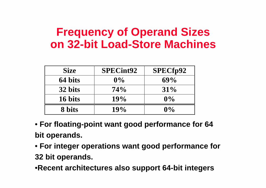
Frequency of Operand Sizeson 32-bit Load-Store Machines

Size SPECint92 SPECfp9264 bits 0% 69%32 bits 74% 31%16 bits 19% 0%8 bits 19% 0%

• For floating-point want good performance for 64 bit operands. • For integer operations want good performance for 32 bit operands. •Recent architectures also support 64-bit integers

Instruction Encoding• Variable

– Instruction length varies based on opcode and addre ss specifiers– For example, VAX instructions vary between 1 and 53 bytes, while x86

instruction vary between 1 and 17 bytes. – Good code density, but difficult to decode and pipel ine

• Fixed– Only a single size for all instructions (including simple ones)– For example, DLX, MIPS, Power PC, Sparc all have 32 bit instructions– Not as good code density, but easier to decode and pipeline: simpler HW

• Hybrid– Have multiple format lengths specified by the opcod e– For example, IBM 360/370, Intel x86– Compromise between code density and ease of decode

• Summary :– If code size is most important, use variable format .– If performance is most important, use fixed format .

Compilers and ISA

• Compiler Goals– All correct programs compile correctly– Most compiled programs execute quickly– Most programs compile quickly– Achieve small code size– Provide debugging support

• Multiple Source Compilers– Same compiler can compile different languages

• Multiple Target Compilers– Same compiler can generate code for different machi nes

Compilers Phases

• Compilers use phases to manage complexity– Front end

» Convert language to intermediate form (RTL)– High level optimizer

» Procedure inlining and loop transformations– Global optimizer

» Global and local optimization, plus register alloca tion– Code generator (and assembler)

» Dependency elimination, instruction selection, pipeline scheduling

Designing ISA to Improve Compilation

• Provide enough general purpose registers to ease register allocation ( more than 16).

• Provide regular instruction sets by keeping the operations, data types, and addressing modes orthogonal

– e.g. data types: 8-,16-,32-bit integer, IEEE FP standard

• Provide primitive constructs rather than trying to map to a high-level language.

• Simplify trade-offs among alternatives. • Allow compilers to help make the common

case fast

RHK.S96 44

ISA Summary• Use general purpose registers with a load-store

architecture. • Support these addressing modes: displacement,

immediate, register indirect.• Support these simple instructions: load, store, add ,

subtract, move register, shift, compare equal, compare not equal, branch, jump, call, return.

• Support these data size: 8-,16-,32-bit integer, IEE E FP standard.

• Provide at least 16 general purpose registers plus separate FP registers and aim for a minimal instruction set.