Learning Good Features for Active Shape Models

Nuria Brunet Francisco Perez Fernando De la TorreRobotics Institute, Carnegie Mellon University, Pittsburgh, Pennsylvania 15213.

Abstract

Active Shape Models (ASMs) are commonly used tomodel the appearance and shape variation of objects in im-ages. This paper proposes two strategies to improve speedand accuracy in ASMs fitting. First, we define a new cri-terion to select landmarks that have good generalizationproperties. Second, for each landmark we learn a subspacewith improved facial feature response effectively avoidinglocal minima in the ASM fitting. Experimental results showthe effectiveness and robustness of the approach.

1. IntroductionActive Shape Models (ASMs) [3, 2] have proven to be

a powerful tool to model the shape and appearance of faces

in images. There are two key components in ASMs: the

learning component, that uses Principal Component Analy-

sis (PCA), and the fitting process, typically done with some

greedy search [2]. Although widely used, two undesirable

effects might occur when using PCA to learn a generic

model of an object’s appearance. First, the location of the

parameters (e.g. translation) fails to correspond to the loca-

tion of the object (e.g. face). Second, many local minima

may be found. Even if a gradient descent algorithm is ini-

tialized close to the correct solution, the occurrence of local

minima is likely to divert convergence from the desired so-

lution. For instance, consider fig. (1.a), where a face has

been labeled with 68 landmarks. For each landmark, a PCA

model that preserves 80% of the energy is computed from

600 training images. Figure (1.b) shows the surface of the

reconstruction error (distance from the subspace) for differ-

ent translations (32 × 32 pixels) around the position of the

landmark (black dot). The region of this particular land-

mark is a good feature because its response has only one

local minimum in the expected location. On the other hand,

there are regions that are not well suited for detecting facial

features in new images. For instance, consider fig. (1.c) that

shows the error surface of a landmark in the outline of the

face. The error surface has multiple local minima and none

in the position of the labeled landmark. In this paper, we

propose a method to learn a subspace that improves the sur-

Figure 1. a) Face image labeled with 68 landmarks. b) Reconstruc-

tion error (i.e. distance from the subspace) in a 32×32 pixels area

around a landmark in the lower part of the nose. The black dot de-

notes the hand labeled position of the landmark. c) Reconstruction

error around an outline landmark. d) Reconstruction error around

the same landmark as subplot c after learning better features.

face response, see fig. (1.d). That is, the new error surface

has fewer local minima and it has the global minimum on

the labeled place. The two main contributions of the paper

are: (1) describe a new criterion to select good regions that

generalize well for ASMs. (2) learn a subspace that explic-

itly reduces the number of local minima.

The rest of the paper is organized as follows. Section 2

reviews previous work on ASMs. Section 3 proposes a new

criterion to select good regions to track. Section 4 describes

a method to learn a subspace that provides good error sur-

faces to fit ASMs. Section 5 presents experimental results.

2. Previous work

ASMs [2] build a model of shape variation by perform-

ing PCA on a set of landmarks (after Procrustes analysis).

For each landmark the Mahalanobis distance between the

sample and mean texture is used to assess the quality of

206 2009 IEEE 12th International Conference on Computer Vision Workshops, ICCV Workshops978-1-4244-4441-0/09/$25.00 ©2009 IEEE

fitting to a new shape. The fitting process is performed

using a local search along the normal of the landmark.

Later, the new positions are projected onto the non-rigid ap-

pearance basis and rigid transformations. These two steps

are alternated until convergence. Recently, Cristinacce and

Cootes [4] introduced extended ASMs with Constrained

Local Models that compute local responses with the learned

templates of the appearance model. CLM has proven to be

a more robust fitting procedure than ASM and AAM.

Although ASMs are widely used, they suffer from large

sensitivity to local minima. Several strategies and methods

to improve fitting have been proposed: Using multiresolu-

tion schemes [2] or Multiband filters [5, 1] have been pro-

posed to improve fitting and generalization in Active Ap-

pearance Models (AAMs). Wimmer et al. [10] propose

a method to learn one dimensional convex error functions

as combinations of Haar-like features. De la Torre and

Nguyen [8] learned a weighted subspace for AAMs that ex-

plicitly avoids local minima in its fitting. Recently, Wu et al.

[11] proposed avoiding local minima in discriminative fit-

ting of appearance models by learning boosting with ranked

functions. Although these methods show significant perfor-

mance improvement, they do not provide a selection mech-

anism for regions that generalize well. Moreover, methods

such as [8, 11] can not guarantee avoiding local minima in

all the search space because they only impose constrains in

some sampled points. Our method differs from previous lit-

erature in two aspects: (1) define a new criterion to select

good regions that generalize well for ASMs, (2) propose a

2D supervised PCA method that learns a good error surface

to fit ASMs.

3. Selecting good regions for fitting ASMsShi and Tomasi [9] present a method to select good fea-

tures to track. The features (pixels) are selected based on

the spatial and temporal statistics of the initial frame and

current frame. Similarly in spirit, in this section, we pro-

pose a method to select good regions for ASMs based on

local minima properties of the surface error.

Given a basis for an appearance model B ∈ �d×k (e.g.

PCA), and a region in an image di (see notation 1) (e.g. 32×32 pixels), the optimal placement of the landmark (x, y) in

the ASM search is obtained by minimizing:

min(a1,a2)

||d(x+a1,y+a2)i − μ−Bci||22||d(x+a1,y+a2)

i ||22(1)

where (a1, a2) are the translational parameters and ci the

1Bold capital letters denote a matrix D, bold lower-case letters a col-

umn vector d. dj represents the j column of the matrix D. dij denotes

the scalar in the row i and column j of the matrix D and the scalar i-th el-

ement of a column vector dj . All non-bold letters will represent variables

of scalar nature. ||x||2 =√

xT x designates Euclidean norm of x.

appearance coefficients. d(x+a1,y+a2)i denotes a region

around the (x+a1, y+a2) position. Searching over the co-

efficients ci and the translations (a1, a2) that minimize eq.

(1) generates a local error surface (e.g. fig. (1.c)). The num-

ber and position of local minima on the surface depend on

many factors, such as: how well PCA generalizes, robust-

ness to undesirable noise, number of bases, or the chosen

representation (e.g. graylevel, gradients). Not all regions

contribute equally to the performance of the ASM. In order

to select good regions to track, it is necessary to define a cri-

terion based on local minima properties of the error surface.

To quantitatively compare the regions’ responses, we

compute three error surface statistics with different patch

sizes and PCA energies:

• Number of minima. The amount of local minima on

the error surface is calculated by counting the number

of points with a sign change in the x and y derivatives

and positive second derivative.

• Distance between the global minimum and the ex-

pected position of the landmark.

• Distance between the global and closest minimum.

To compute these statistics a local PCA model for each

of the 68 landmarks is built, see fig. (2.a). The landmarks

have been manually labeled in 600 frontal face images (neu-

tral expression) from the CMU Multi-pie database [7], after

Procrustes analysis [2]. The local PCA model is computed

for different patch sizes, 20×20, 30×30 and 60×60 pixels,

and for three different energies: 60%, 70% and 80%.

Figure 2. a) 68 landmarks. b) Best 34 patches to track according

to eq. 2. The number indicates order of the best regions.

A good region for ASMs is considered if the global min-

imum is close to the expected location of the landmark. Fig.

(3) shows the mean and std of the distance for each of the 68landmarks. These statistics are computed in 320 testing im-

ages (not in the training). As expected, the distance between

the global minimum to the desired position is inversely pro-

portional to the energy level. That is, the distance decreases

if energy increases. On the other hand, the higher the PCA

energy the more likely it is to have more local minima in

the patch, see fig. (4). Hence, there is an energy trade-off

207

between having a good localization and the density of local

minima.

Figure 3. Mean and standard deviation of the distance from the

global minimum to the expected position of the landmark. Also

the standard deviation is plotted. The statistics are computed for

two PCA energies, 60% and 80%. Patch number corresponds to

the numbers in fig.(2.a).

The number of local minima also depends on the size

of the patch (20 × 20, 30 × 30 and 60 × 60), see fig. (5).

Moreover, the density of local minima decreases with the

size of the patch. However, the computational complexity

of the algorithm scales quadratically with the dimensions

of the patch. A good trade-off between computational com-

plexity, localization and density of local minima is found by

using 30× 30 pixels (80% of energy in PCA).

Figure 4. Mean and standard deviation of the number of local min-

ima for each of the 68 patches. The statistics are computed for two

PCA energies, 60% and 80%. See fig.(2.a).

Independently of the patch size or energy, there are some

regions that generalize better than others. For instance, the

patch number 34, situated below the nose, has the smallest

average number of local minima. Moreover, the distance

between the global minimum and the expected location of

the landmark is small. In contrast, the patch number 3 sit-

uated on the left side of the outline is particularly difficult

to track. It has several local minima and the distance from

the global minimum to the labeled position is large. We

propose to select those regions that minimize μpatch:

μpatch = μ1patch+ μ2patch

(2)

σpatch =μ1patch

σ1patch+μ2patch

σ2patch

μ1patch+μ2patch

where μ1patch,σ1patch

are the mean and variance of the

distance between the global minimum to the labeled one.

Similarly, μ2patch,σ2patch

are the mean and variance of the

number of local minima. We have assumed that the distance

and density of local minima are independent Gaussian ran-

dom variables. Fig. (2.b) shows the best 34 patches ranked

using eq. (2). The best patches are situated on the mouth,

nose, eyes and some on the eyebrows.

Figure 5. Mean number of local minima for each of the 68 patches.

The statistics are computed for 3 patch sizes, 20×20, 30×30 and

60 × 60 pixels. See fig.(2.a).

4. Learning good features for ASMsThis section investigates a new methodology to build

good subspace features to avoid local minima in ASMs.

4.1. Learning to model the error surface

A region with good generalization properties, ideally,

would have a unique local minimum in the expected po-

208

sition of the landmark. A reasonable approximation would

be the response of an inverted Gaussian (see fig.(6)) in a

neighborhood of a particular position (x, y). Other convex

non-symmetric functions are also possible.

Figure 6. Inverted Gaussian response function (R) (32×32 pixels).

To encourage the error surface in a neighborhood to be

close to an ideal one, we minimize:

E =n∑

i=1

∑(x,y)

(αirx,y + oi − ||d(x,y)i − μ−Bci||22||d(x,y)

i ||22)2 (3)

with respect to B,C, αi and oi ∀i. rx,y is the desired re-

sponse of the Gaussian (see fig.(6)) at the location (x, y),αi and oi are scale and offset factors of the ideal error sur-

face for each image di. B ∈ �d×k and C ∈ �k×n are

the subspace bases and coefficients respectively. PCA is

an unsupervised learning technique; however, eq. (3) is a

supervised-PCA problem. Eq. (3) aims to find a subspace

that has a global minimum where the landmark has been

placed, and at the same time encourages the response in a

certain neighborhood to be as Gaussian as possible.

At this point, it is worth pointing out three important

aspects: (1) observe that we are only avoiding local min-

ima using translational parameters. This might be seen as

a limitation of the method, but it does not need to be. The

optimization can handle small rotation and translation per-

turbations. If the ASM is used for tracking, the rotational

and scale parameters can be incrementally computed after

the convergence of the ASM. Normalizing the new image

with the rotational and scale parameter will allow the ASM

to search at a similar scale and rotation as it was previously

learned. However, if the ASM is used for detection an ap-

proximate scale has to be given (e.g. from a face detector

in the case of faces). (2) In our case, the inverted Gaus-

sian has been chosen as an ideal error function. However,

there are many other desirable convex error functions. A

simple approach to have more accurate modeling of the er-

ror function will be to select for each landmark and from a

set of prototypal function the one with less error. However,

in our experimental validation, it has been always observed

that the optimization of eq. (3) with an inverted Gaussian

always improves local minima properties of the error sur-

face. (3) Observe that if for each landmark the resulting

error surface is locally convex with the global minimum in

the expected place, any search algorithm (e.g. gradient de-

scent, simplex) will succeed in fitting the ASM (assuming

the shape model generalizes correctly). Observe that if few

points improve their fitting properties, this will imply that

that standard search mechanism for ASM will also improve

performance.

4.2. Optimization

Our aim is to obtain a new subspace B able to minimize

eq. (3). Unlike PCA, there is no closed form solution for

the optimization of eq. (3). We alternate between solving

for αi, oi in closed form, and performing gradient descent

w.r.t. B. These steps monotonically decrease the error of

E. The gradient descent updates of B are given by:

Bn+1 = Bn − ηG G = ∂E∂B (4)

∂E∂B =

∑ni=1

∑x,y

2tx,y

||d(x,y)i ||22

(d(x,y)i − μ−Bc(x,y)

i )c(x,y)i

T

tx,y = αirx,y + oi − fx,y fx,y = ||d(x,y)i −μ−Bc

(x,y)i ||22

||d(x,y)i ||22

The closed form solution for αi, oi is given by:

[ ∑x,y r2

x,y

∑x,y rx,y∑

x,y rx,y

∑x,y 1

] [αi

oi

]=

[ ∑x,y fx,yrx,y∑

x,y fx,y

](5)

The major problem with the update of eq. (4) is deter-

mining the optimal η. In our case, η is found with a line

search strategy [6], minimizing E(B − ηG). It can be

shown that the optimal η corresponds to the solution of the

following third order polynomial:

aη3 + bη2 + cη + d = 0 (6)

a =∑n

i=i

∑x,y ν2 b =

∑ni=i

∑x,y 3ων

c =∑n

i=i

∑x,y 2ω2 − νtx,y

d = −∑ni=i

∑x,y ωtx,y

ν = c(x,y)i

TGT Gc

(x,y)i

||d(x,y)i ||22

ω = c(x,y)i

TGT (d

(x,y)i −μ−Bc

(x,y)i )

||d(x,y)i ||22

Experimentally, we found the roots of the polynomial

always to be one real and two complex conjugate. If the

three of them turn out to be real, the one that has lower

error (E) value would be chosen. After each iteration, we

orthonormalize the basis (i.e. Bnew = B(BT B)−0.5).

Minimizing eq. (3) with respect to B is a non-convex op-

timization problem prone to local minima. Without a good

initial estimate of B, the previous optimization scheme

might converge to a local minimum. To get a reasonable

209

estimation, we initialize B with the PCA solution. More-

over, we start from several random initial points and select

the solution with minimum error after convergence.

5. ExperimentsThis section reports several experiments that show the

benefits of our method for selecting and building better fea-

tures for facial feature detection.

5.1. Selecting good regions to fit ASMs

In this experiment, we test the ability of the ASM to de-

tect facial features in frontal faces. We compare an ASM

built with 68 landmarks and an ASM built with half of the

regions (34). The best regions to build an ASM are selected

based on the statistics of the error surface described in sec-

tion 3 using eq. (2). It is important to note that the images

used to compute the statistics are not included in the train-

ing set. To ensure that the displacement error is similar in all

the regions of the face, we have selected half of the patches

for each region (fig. 7).

Figure 7. Best patches for each region of the face (outline, eye-

brows, nose, eyes and mouth).

The algorithms are compared using 100 testing images

(previously labeled). We perturb the rigid and non-rigid

transformation and let the ASMs converge. Each PCA

model is created using a patch of 30 × 30 pixels around

the landmark [5]. Fig. (8) shows the perturbed and the re-

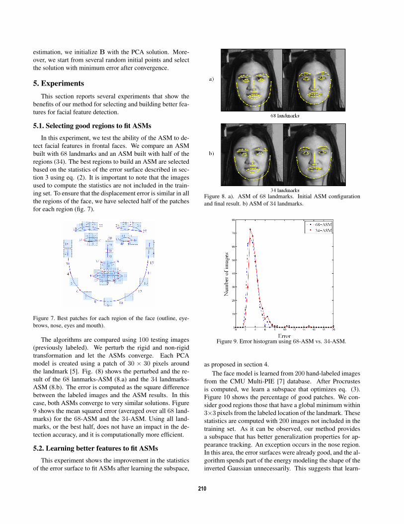
sult of the 68 lanmarks-ASM (8.a) and the 34 landmarks-

ASM (8.b). The error is computed as the square difference

between the labeled images and the ASM results. In this

case, both ASMs converge to very similar solutions. Figure

9 shows the mean squared error (averaged over all 68 land-

marks) for the 68-ASM and the 34-ASM. Using all land-

marks, or the best half, does not have an impact in the de-

tection accuracy, and it is computationally more efficient.

5.2. Learning better features to fit ASMs

This experiment shows the improvement in the statistics

of the error surface to fit ASMs after learning the subspace,

Figure 8. a). ASM of 68 landmarks. Initial ASM configuration

and final result. b) ASM of 34 landmarks.

Figure 9. Error histogram using 68-ASM vs. 34-ASM.

as proposed in section 4.

The face model is learned from 200 hand-labeled images

from the CMU Multi-PIE [7] database. After Procrustes

is computed, we learn a subspace that optimizes eq. (3).

Figure 10 shows the percentage of good patches. We con-

sider good regions those that have a global minimum within

3×3 pixels from the labeled location of the landmark. These

statistics are computed with 200 images not included in the

training set. As it can be observed, our method provides

a subspace that has better generalization properties for ap-

pearance tracking. An exception occurs in the nose region.

In this area, the error surfaces were already good, and the al-

gorithm spends part of the energy modeling the shape of the

inverted Gaussian unnecessarily. This suggests that learn-

210

ing should only be applied to regions with bad local minima

statistics.

Figure 10. Percentage of desired response of error surface for two

models; with and without learning good features.

Fig. (11) left shows the initial PCA-error surface for two

patches. Fig. (11) right shows the results after our algorithm

is applied. One patch corresponds to the eye region (40) and

the other one to the mouth (63).

Figure 11. Reconstruction error surface around (11 × 11 pixels)

before (left) and after (right) learning good features to track.

5.3. Detection using improved features

This section tests the ability of ASMs to fit new untrained

images. As in section 5.2, a PCA model for each of the 68landmarks is built from 200 frontal images from the Multi-

pie [7] database. We use 100 testing images and randomly

perturb the manual labels by a maximum of 12 pixels.

Fig. 12 shows the average error distribution for PCA and

our model for 100 testing images. Both results are obtained

after 2 iterations using a search window of 11×11 pixels for

each landmark. As we can see, our method achieves lower

error than PCA.

Acknowledgements This work has been partially sup-

ported by the U.S. Naval Research Laboratory under Con-

tract No. N00173-07-C-2040. Any opinions, findings and

Figure 12. Error distribution using PCA and our method.

conclusions or recommendations expressed in this material

are those of the authors and do not necessarily reflect the

views of the U.S. Naval Research Laboratory.

References[1] H. Bischof, H. Wildenauer, and A. Leonardis. Illumination

insensitive recognition using eigenspaces. Computer Visionand Image Understanding, 1(95):86 – 104, 2004.

[2] T. Cootes and C. Taylor. Statistical models of appearance for

computer vision. In Tech. Report. University of Manchester,

2001.

[3] T. F. Cootes, C. J. Taylor, D. H. Cooper, and J. Graham.

Active shape models- their training and application. Com-puter Vision and Image Understanding, 61(1):38–59, Jan-

uary 1995.

[4] D. Cristinacce and T. Cootes. Automatic feature localisation

with constrained local models. Journal of Pattern Recogni-tion, 41(10):3054–3067, 2008.

[5] F. de la Torre, A. Collet, J. Cohn, and T. Kanade. Filtered

component analysis to increase robustness to local minima

in appearance models. In International Conference on Com-puter Vision and Pattern Recognition, 2007.

[6] R. Fletcher. Practical methods of optimization. John Wiley

and Sons., 1987.

[7] R. Gross, I. Matthews, J. F. Cohn, T. Kanade, and S. Baker.

The cmu multi-pose, illumination, and expression (multi-

pie) face database. Technical report, Carnegie Mellon Uni-

versity Robotics Institute.TR-07-08, 2007.

[8] M. Nguyen and F. de la Torre. Local minima free parame-

terized appearance models. In International Conference onComputer Vision and Pattern Recognition, 2008.

[9] J. Shi and C. Tomasi. Good features to track. In IEEE Con-ference on Computer Vision and Pattern Recognition, 1994.

[10] M. Wimmer, F. Stulp, S. J. Tschechne, and B. Radig. Learn-

ing robust objective functions for model fitting in image un-

derstanding applications. In Bristish Machine Vision Confer-ence, 2006.

[11] H. Wu, X. Liu, and G. Doretto. Face alignment via boosted

ranking model. In Proceedings of IEEE Conference on Com-puter Vision and Pattern Recognition, 2008.

211