Learning by Driving: Productivity Improvements by New York City Taxi Drivers1

Kareem Haggag

University of Chicago

Brian McManus

University of North Carolina

Giovanni Paci

Columbia University

June 2014

Abstract:

We study learning by doing (LBD) by New York City taxi drivers, who have substantial

discretion over their driving strategies and receive compensation closely tied to their success in

finding customers. The breadth of the data, which cover each individual fare during 2009, allows

us to document significant learning while controlling for unobservable factors that often

constrain the LBD literature. In addition, we use the data’s detail on fares’ locations and times to

show that new drivers lag behind experienced drivers to a greater extent in more difficult

situations, and that new drivers benefit from both general and neighborhood-specific experience.

Keywords: learning by doing, specific human capital, taxis, big data

JEL Codes: D24, D83, J24, L92

1 Contact information: kareem.haggag@chicagobooth.edu, mcmanusb@unc.edu, and gp2282@columbia.edu. We thank Ray Fisman, Jonas Hjort, Supreet Kaur, Kiki Pop-Eleches, Bernard Salanie, Chad Syverson, James Roberts, and several seminar audiences for helpful comments.

1

1. Introduction

Learning by Doing (LBD) is a widely studied economic phenomenon, with potential impacts on

macroeconomic growth, market structure evolution, and individuals’ wage dynamics. Prior

studies of LBD have examined productivity improvements by individual workers, as well as

“organizational learning” which describe more complex improvements which may not be

embodied in a single agent. While some exceptions exist, the empirical literature generally

focuses on manufacturing settings, with LBD captured through reductions in unit cost as a firm

or worker accumulates experience. In these cases, while production improvements may be strong

and clear, it can be difficult to learn which agents are improving their capabilities, what activities

are being improved, and how strongly individual agents are encouraged to find improvements.

We provide new evidence on LBD that addresses some of these gaps in the literature. We

use a highly detailed dataset of New York City (NYC) yellow taxi drivers to study how drivers

make improvements overall, how their performance varies across measurably different

situations, and how general and specific experience makes different contributions to driver

performance. Taxi service in NYC is characterized by two features that make it an especially

interesting setting for studying LBD. First, drivers have substantial discretion in how they search

for new customers, and their compensation is very closely tied to the earnings they collect

through customers’ fares. Drivers’ agency in their own production makes them similar to

entrepreneurs, searching for the next fruitful business opportunity. Second, drivers operate in an

environment that lends itself to a relatively clean study of learning. While other LBD studies

often contend with isolating productivity improvements from confounding factors such as scale

economies, improvements in inputs, and shifts in input prices, by contrast all taxi drivers

essentially use the same capital equipment, work in the same demand and cost environment, and

charge the same prices.

We perform our analysis using data on all 171 million NYC yellow taxi rides during the

full 2009 calendar year. Our main analysis features a sample of 7,664 drivers who worked an

average of 176 shifts over the year. Among these drivers we identify 3,298 as “new” based on

their first day in the 2009 data (after March 1st), and other criteria. Our main measure of overall

experience is driver shifts (i.e. full days of work), although it is also possible to use finer

divisions such as the driver’s cumulative number of drop-offs. We measure driver output through

fare earnings per hour. By incorporating the activity of experienced drivers together with new

2

ones, we are able to control for variation in the earning opportunities across each individual hour

of our dataset; this allows us to eliminate bias due to selection effects of new drivers into lower-

demand shifts. We find that a new driver’s productivity is about 8.1% less than an experienced

driver’s when the new driver is in his first shift. A new driver’s productivity increases by 0.19%

for each 10% increase in the number of shifts, and by a driver’s 70th shift he earns as much as an

experienced driver. New drivers’ earnings continue to grow, and by the new driver’s 120th shift

his average earnings are 1% above those of the average driver who entered the industry before

2009.

Our most novel results come from the opportunity to observe the time and location of

every pick-up and drop-off of each ride during 2009. We use census boundaries to divide New

York City’s five boroughs into a collection of 220 neighborhoods, and further divide the week

into 168 hour-long blocks. For each neighborhood and each hour of the week, we use a sample

of 17,463 experienced drivers (i.e. all experienced drivers not included in our analysis sample) to

compute the expected earnings of a driver following a drop-off in a particular setting. These

statistics are useful in describing whether certain situations represent “easy” or “hard” earnings

opportunities. We find that new drivers earn considerably less in more difficult situations.

Following a drop-off in one of the most difficult location-hours, a driver in his first shift will

earn 14% less than an experienced driver in the same situation, but brand new drivers earn only

1.5% less than experienced drivers in the easiest settings. Despite the large gap in initial earnings

in difficult situations, new drivers’ earnings improve fastest there and erase the gap with

experienced drivers after 136 shifts.

The time- and location-specific data also allow us to compute a new driver’s share of

experience in each neighborhood and portion of the day (and the intersection of these). We

estimate that the importance of location-specific experience is comparable to general experience

for new drivers’ earnings. A new driver whose experience is relatively concentrated (75th

percentile) within a neighborhood has expected earnings that are 4% greater than new drivers

with a smaller share (25th percentile) of experience in a given neighborhood. Moreover, time-

specific experience at a location explains a substantial share of the benefit from local experience.

Our analyses of task difficulty and general versus specific experience rely on two simple

but powerful identification opportunities. First, we observe new drivers visiting a variety of

locations a large number of times. On average, a driver makes 23 drop-offs per shift. Relative to

3

the labor literature, which relies on relatively infrequent job switches to disentangle the effects of

specific versus general human capital, we observe substantially more chances to see how a driver

performs in different tasks. The second opportunity comes from the randomness introduced to

task selection through customer-selected destinations. While drivers are in control of the

neighborhoods in which they look for new customers, they do not control the selected

destination. The customer drops the driver into some location which could be easy or hard, or

within which the driver has little or substantial prior experience. We contrast this with the usual

endogeneity concerns about the motivation for workers to switch jobs within their careers, which

may bias estimates of job-specific human capital in studies that use labor panel data.

Our results join a large empirical literature on LBD; see Thompson (2010 and 2012) for

surveys of the field. Several recent papers have grappled with the same issues that interest us.

Jovanovic and Nyarko (1995) consider potentially-bounded learning by individual agents in a

variety of occupations. Hatch and Mowry (1998) and Hendel and Spiegel (2014) use extremely

fine data on production improvements in manufacturing, and they discuss the distinction among

improvements that coincide with deliberate changes to production processes, small “tweaks” to

production, and passive learning which occurs automatically. Our consideration of

heterogeneous tasks is related to Levitt et al. (2013), who use a variety of measures on

production improvements within a single auto manufacturer. More common in the literature are

studies that aggregate activity across diverse settings and offer some controls for this diversity

without directly studying it; examples include Kellogg’s (2011) study of relationship-specific

LBD across a variety of Texas oilfields, and Thompson’s (2001) estimation of separate ship yard

productivities within an investigation of aggregated learning across yards. Examples of research

that allow for differences in learning speeds across agents include Rockart and Dutt’s (2013)

study of equity-underwriting projects, and Pisano et al.’s (2001) study of hospitals’

improvements in cardiac surgery.

Our paper also relates to a labor literature that studies general and (firm- or task-) specific

experience by workers. Similar to our exercise, Shaw and Lazear (2008) use direct output

measures to study learning at the individual-worker level. They find that new installers of

automobile windshields have steep productivity-tenure curves that are attributed to both learning

and effort, although Shaw and Lazear cannot distinguish between general and specific

experience in their exercise. Also closely related to our paper is Ost (2014), who studies how

4

elementary school teachers’ general and grade-specific experience affect classroom productivity

as measured through reading and math test scores. Additional prior studies of task-specific

experience include Gathmann and Schonberg (2010), who use German panel data which span

many occupations, and Clement et al. (2007), who study variation in forecasting accuracy in a

cross-section of financial analysts.

The rest of our paper is organized as follows. In Section 2 we provide an overview of the

NYC taxi market, including the various activities that are tracked by our primary data source, the

NYC Taxi and Limousine Commission (TLC). In Section 3 we provide an overview of the data.

Section 4 contains our empirical analysis, and Section 5 concludes.

2. The New York City taxi market

We study driving activity in New York City’s yellow taxicabs. These taxis serve customers who

hail from the street, plus taxi queues at airports, train stations, and hotels. They are not permitted

to accept customers in any other way. Other types of for-hire vehicles (e.g. town cars and

limousines) serve the market for pre-arranged and radio-dispatched transportation. During our

sample period of 2009, there were 13,237 yellow cab taxi licenses (“medallions”) and about

40,000 additional for-hire vehicles in New York City. Each medallion corresponds to a single

yellow taxi, which may be controlled by an owner-operator, a firm with a fleet of cabs, or an

authorized leasing agent. The taxis are operated by drivers licensed by New York’s Taxi and

Limousine Commission; the number of drivers increased from 46,409 to 48,521 during 2009.

The change in number of drivers combines the separate effects of attrition, the entry of new

drivers, and the potential return of experienced drivers who ended extended absences from the

market.

Taxi drivers enter the market through a variety of avenues. Based on conversations we

have had with taxi fleet managers, it appears that very few drivers are “seasonal” in the sense

that they take multi-month breaks from driving a taxi before returning to the job. Schaller (2006)

reports that, in 1991, 20% of TLC license applicants drove professionally in their previous job,

with 44% of applicants having ever held a professional driving position (in New York or

anywhere in the world). Restaurants and food service firms provide the second-largest share

(15%) of previous employment. To obtain a TLC license, drivers are required to: hold a valid

DMV license; attend either a 24-hour or 80-hour Taxicab School course; and pass tests on New

5

York geography, TLC rules, and English language proficiency. New and experienced drivers are

likely to differ on personal characteristics and performance. Schaller (2006) reports that the

median experienced driver is about ten years older than a typical newly-licensed driver, and

experienced drivers receive fewer complaints for service problems such as refusing passengers,

overcharging, treating passengers rudely or abusively, or driving unsafely. Driver experience is

also negatively correlated with the number of accidents and traffic violations (Schneider, 2010).

Taxi earnings and costs are structured so that it is in the driver’s interest to maximize fare

earnings during a shift. Drivers keep all fares and tips. Fares are accrued as a function of ride

distance and duration, and may include surcharges for nighttime rides, peak weekday rides, and

destinations at airports or outside of New York City’s five boroughs. Drivers’ costs vary

depending on their ownership of the taxis they drive. All drivers pay for their own gas ($5,000-

$10,000 per year), annual TLC fees ($100), and DMV/TLC fines for driving infractions. Drivers

who lease their vehicles will pay a per-day or per-week flat fee; these fees were about $100 per

day in 2009. Owner-operators pay for annual maintenance and repair ($4,000-$10,000/year),

insurance ($7,000-$13,000/year), and licensing fees ($1,000/year). On average, a driver’s take-

home pay is 57% of revenue, with the rest divided among expenses paid by the driver and taxi

owner (Schaller 2006). Driver earnings vary with the time of day and day of the week, so some

shifts are more lucrative than others. Experienced drivers are generally sorted into the more

valuable shifts; we document this pattern below. In our conversations with fleet managers we

have learned that this is largely due to seniority rules for the assignment of drivers to shifts.

3. Data

3.1 Sample construction

The data we use in analysis are derived from a fare-by-fare database of yellow taxi activity from

the full 2009 calendar year. These data are collected by the TLC as part of an effort to monitor

the activity of taxis and their drivers in the NYC area. The database includes all fares for licensed

NYC cabs, even if one or both endpoints of a fare occur outside of the city’s five boroughs.

We begin with a full database of 171 million observed fares received by 41,256 drivers.

Each observation includes a unique driver-specific index, the longitude, latitude, date, and time

of the ride’s pick-up and drop-off, and payments to the driver. Date and time are recorded to the

6

second, and longitude and latitude are recorded through on-board GPS.2 The total payment is

broken down into the fare, surcharges, tip when the payment is via credit card, and MTA tax.

The combination of driver identification codes and specific ride data allow us to construct a

complete history of each individual driver’s activity during 2009. Following Farber (2005), we

define a shift as a succession of rides with breaks between rides no longer than 5 hours. We then

track each driver’s total fare earnings per shift, the shift’s duration, and running counts of the

driver’s numbers of drop-offs in each neighborhood and neighborhood-time of day combination.

We also construct statistics within selected hours of a shift. The measures include for each

driver: fare earnings in the hour, percentage of time spent idle or slack (i.e. without a passenger),

the number of miles driven, the number of fares collected, and the average driving speed.

Unfortunately we do not have additional information about the drivers’ personal characteristics,

employer’s identity, contract terms, or costs.

We clean and organize the data in order to conduct analysis of new versus experienced

drivers. Our primary metric for experience is the number of shifts worked. We remove drivers

and shifts that are unlikely to represent the production efforts of a regular driver in the market. In

particular, we drop drivers who are associated with fewer than 100 fares, shifts associated with

more than one unique car identifier, and shifts that were shorter than 2 hours or longer than 15

hours. This reduces the dataset to 156 million observations. 86% of the data reduction comes

from the elimination of very long shifts, and 9% is due to drivers who use multiple cars in a

single shift.

Next, we separate drivers into groups by their level of experience. We identify 27,519

drivers who first appeared in the data on or before January 15, 2009. Of these drivers, we retain

21,819 who worked at least 100 shifts between January 1 and December 31, and additionally

worked at least 20 shifts before March 1. These drivers are likely to have pre-2009 experience in

the market, while also working in the market with enough frequency to maintain their stock of

knowledge. To maintain tractability of the data, we select a 20% random sample of these drivers

as our “experienced” drivers in the analysis described below.

2 Longitude and latitude are reported to one-foot precision, but the presence of tall buildings and other technical challenges is likely to distort these values somewhat. Small errors in location data will not affect our estimates, which use areas of several city blocks as the finest descriptors of taxi location.

7

From the collection of drivers who fail the criteria for experienced drivers, we identify a

subset that are likely to have entered the NYC taxi workforce in 2009 as new or inexperienced,

and work with sufficient frequency to indicate an intention to function as a full-time taxi driver

in the market. To identify these new drivers, we isolated the sample to 5,310 drivers that were

first observed in the data on or after March 1, 2009. Among these drivers, we select the 3,298

who worked at least 50 shifts between their entry date and December 31, 2009. It is possible that

some of these drivers have prior experience in the NYC taxi market, but we cannot measure the

size of this effect in the data. To address the possibility that some of these drivers are seasonal

workers, we have performed additional analysis (discussed below) on drivers who are subject to

stricter inclusion criteria; our results are largely unchanged. In addition, we have experimented

with a variety of thresholds for the first day of work by new drivers and the total number of shifts

driven, and again the results are unaffected. To complete the selection of drivers and shifts for

analysis, we limit both the experienced and new driver samples to shifts that start between March

1 and December 31, 2009.

We use the longitude and latitude information in the fare database to identify the NYC

geographic region in which each pick-up and drop-off occurs. We divide the market in two ways.

First, we use the boundaries of Public Use Micro Areas (PUMAs) to identify 59 regions within

the city’s five boroughs. PUMAs represent a fairly coarse division of the city; for example one

PUMA is defined by the portion of Manhattan west of Central Park and approximately bounded

by the Park’s north and south edges. Second, we use the boundaries of 220 Neighborhood

Tabulation Areas (NTAs), which are mostly nested within PUMAs and correspond more closely

to conventional views of NYC neighborhoods. For example, the Lincoln Square area is a distinct

NTA within the Manhattan PUMA described above.

We use the geography data in two ways. First, we use a random sample of experienced

drivers3 to construct statistics on driver performance within each NTA-hour and PUMA-hour

combination within a week (i.e. for each region a separate measure is constructed for each of

7×24=168 unique hours in the week). Using the fare-level data, we calculate each experienced

driver’s total earnings during the 60 minutes following a drop-off in a specified region-hour. We

then average these earnings across all drivers in the same region-hour, thereby computing a

3 We use data from all experienced drivers who are not within the 20% sample that we employ in our main analysis.

8

measure of how locations and times may vary in the earning opportunities available for drivers.4

Some passenger-selected drop-off locations may take the driver to a part of the city where (at a

given time of day) it is especially easy to find the next customer, or perhaps find customers who

are likely to request rides to high-earning areas. With these measures of average earning within

regions and time, we can characterize some situations as “easy” or “hard” production

opportunities, and investigate how new driver performance varies with task difficulty.

Our second use of the geography data is to construct measures of location and location-

time specific experience by new drivers. For all new drivers who are included in our analysis

sample, we maintain a running count of the number of drop-offs that the driver has experienced

in each PUMA and NTA. We also divide the day into four six-hour blocks (11pm-5am, 5am-

11am, 11am-5pm, and 5pm-11pm), and record each driver’s experience in a PUMA or NTA

within each time block. With these drop-off counts, we are able to track the evolution of a

driver’s general and specific experience during the 2009 calendar year. For example, if we are

considering a new driver’s performance following a particular drop-off, we may ask what share

of the driver’s experience comes from dropping-off passengers in the same neighborhood and

during the same portion of the day.

3.2 Summary statistics

Our analysis features two populations of drivers. All of our analysis includes activity by the

3,298 new drivers who meet the selection criteria described above. We also use a 20% random

sample of 4,366 experienced drivers, who act as a comparison group in much of the empirical

analysis. We present summary statistics on the drivers’ productivity in Table 1, separately

reporting activity for experienced drivers, new drivers overall, and new drivers in their first 20

shifts. As in our analysis below, all summary statistics correspond to shifts between March 1 and

December 31, 2009.

We examine several types of productivity variables, including average earnings per hour

and earnings within a specified hour of the shift. We generally focus on the 60 minutes following

4 Before constructing this measure, we first drop all rides that are not followed by at least 4 more rides within the driver’s shift (17.9% of observations), so as not to characterize locations by endogenous shift-ending behavior. We also set the driver’s fare-earnings to missing if equal to zero (to coincide with our rule in the regression analysis). Finally, after constructing the NTA/Hour averages, we drop all NTA/Hours with fewer than 10 observations over the entire sample period (this corresponds to the bottom 10% of the distribution of NTA/Hour observations).

9

a driver’s third drop-off of a shift. For convenience we refer to this period as “hour-R3” in our

text and tables. Hour-R3 roughly overlaps with a driver’s second hour of work. For the median

driver this hour begins at minute 55 of the shift, and drivers at the 25th and 75th percentiles begin

at minutes 39 and 81, respectively. This hour is a microcosm of earning opportunities yet less

likely to be affected by considerations about when to stop working or whether to take long mid-

shift breaks, which may differ between new and experienced drivers.5 This also allows us to look

directly at the pick-up and drop-off times and locations of the driver’s final fare starting

immediately before hour-R3, as well as the pick-up time and location of the next fare. In

computing earnings in the hour following a drop-off, we omit observations in which a driver has

no customers for 60+ minutes. We infer that the driver is on a break, and is not attempting to find

new customers. This rule affects 5% of our observations, and has no substantial effect on the

results described below.

The earnings statistics in Table 1 show that experienced and new drivers collect about the

same value in fares per hour (approximately $26), but the median new driver in his first 20 shifts

earns $1.43 less per hour (5.5%) than the average experienced driver. Similar differences emerge

across experienced and new drivers when we compare other measures of driver activity. Drivers

in their first 20 shifts spend a larger fraction of hour-R3 without a passenger, and the slack time

between their third drop-off and the next pick-up is longer, on average. These differences have

an influence on numbers of miles driven and customers served. Average ride duration is greater

for experienced drivers, despite these drivers taking more customers per hour. Average travel

speed, which is approximately the same across drivers of all experience levels, could capture

both drivers’ ability to navigate congested city streets and the types of passengers and locations

favored by the driver. Any differences displayed among drivers in this table, however, could be

influenced by variation in market conditions when drivers of different experience levels are

working.

In addition to differences in productivity, in Panel B of Table 1 we display some

differences in working practices by new and experienced drivers. We observe new drivers

working fewer shifts per person than experienced ones, but this is largely an artifact of our data

5 An advantage of this variable is that it allows us to partially separate learning from drivers’ habituation to driving conditions, such as sitting for many hours, which may be less likely to be important early in the shift.

10

construction procedure. (Experienced drivers work in the market from March to December, but

new drivers are added gradually during this period.) New and experienced drivers work a similar

proportion of days following their first appearance in the analysis sample. Some notable

differences exist in the number of cars associated with each driver. While our data do not provide

information on drivers’ relationship to cab owners, we observe that experienced drivers are

170% more likely to be paired with a single taxi during the sample period. This suggests that the

proportion of owner-operators and long-term lessees is larger in this population. Taxi ownership

may provide greater flexibility for drivers to choose their own schedules, which can affect

earning opportunities. In Figure 1’s Panel A we display the proportion of pick-ups in our analysis

sample by new drivers across different hours of the day on Tuesdays and (separately) Saturdays,

and we see some variation in when new drivers are more likely to be working.6 The Figure’s

Panel B displays the average number of pick-ups per hour during the same days, and it appears

that new drivers are most common in the market when overall demand is relatively low. These

differences in selection into shift hours highlight the importance of controlling for earning

opportunities across days and hours of the sample period.

In Figure 2 we provide an illustration of how earning opportunities vary across the city,

and to what extent they vary across four different hours on Tuesday and Saturday. We separate

the NTA-hour earnings statistics into quartiles. The first quartile (lightest shading) represents the

lowest average earnings ($19.08 on average) in the hour following a drop-off, and the fourth

quartile (darkest shading) contains the highest average earnings ($33.83). In constructing the

quartiles, we weight the NTA-hour statistics by the frequency with which they occur in the fare-

level data for the new and experienced drivers of the analysis sample. Some NTAs (largely on

Staten Island) are unshaded because fewer than 10 rides terminated in those neighborhoods

during an hour of the week. Lower Manhattan is at its most lucrative around rush hours and on

weekend evenings, while the Bronx contains many neighborhoods in the lowest-earning quartile.

The eastern portions of Brooklyn and Queens have relatively high average earnings, likely

because of their proximity to John F. Kennedy airport, from which the TLC mandated a flat fare

of $45 in 2009.

6 Our use of the analysis sample, with all qualifying new drivers but only 20% of qualifying experienced drivers, inflates the proportion of new drivers relative to the actual share in the market.

11

Some of our empirical analysis relies on an assumption that drivers are randomized into

locations across the city based on the requested destinations of their customers. While drivers

can control where they pick up customers, they do not determine the drop-off location.7 Contrary

to our assumption, if drivers gain expertise in selecting customers who are likely to request rides

to more lucrative drop-off locations, then some of their measured improvements in fares will be

due to the ability to avoid arriving in difficult situations rather than performing well within them.

(This would be a different sort of learning than interests us.) We evaluate our randomization

assumption by investigating whether new and experienced drivers have different outcomes in the

mean earnings of a destination (measured at the NTA-hour and PUMA-hour level). Our results,

which we report in Appendix Table A1, show that once we account for the date, hour, and NTA

in which a ride begins, the expected earnings of the destination are uncorrelated with a driver’s

stock of experience.

4. Empirical analysis

We estimate a set of reduced-form econometric models to satisfy our research objectives. The

models are reduced-form in the sense that they do not model drivers’ choices and how these vary

with experience, but instead we measure how market outcomes (e.g. wages) vary across drivers

with different amounts of experience. It is beyond the scope of this paper to perform a direct

analysis of drivers’ choices, but this is a topic we are studying in ongoing research.

Our first goal is to document overall learning dynamics, and also investigate how

estimating learning can be affected by sample selection or functional form assumptions. We

perform this analysis with a variety of measures of driver productivity, and across a variety of

situations that vary in difficulty. The second goal is to use the data’s geographic detail to

estimate the relative importance of general and specific experience on a driver’s productivity.

We perform our main analysis with a fairly simple econometric framework. Let yit be

driver i’s productivity during shift t. The production measure could be (a function of) fare per

hour during t, fare during a specified hour of shift t, or a measure of the driver’s idle time. The

7 While drivers’ refusals of fares may happen occasionally in practice (and contrary to our assumptions here), this activity is against TLC regulations and can result in the driver receiving a punishment. During our sample period, refusal punishment was $200-$350 for a first offense, $350-500 and a possible 30-day license suspension for a second offense, and a mandatory license revocation for a third offense. The TLC received about 2,000 formal complaints per year in 2009 and 2010.

12

new driver’s experience at shift t is Eit. We generally assume that E is the current shift number

for a new driver, but in some specifications E is the cumulative number of drop-offs that a driver

has completed as of t. We also calculate the share of all drop-offs that occur within each

location-time block combination as of shift t, and we extend E to include these shares. We

measure the impact of E on y with the function g(E;θ), where θ is our main parameter vector of

interest. In some specifications we let g be the natural log of a scalar E, while in others g is a set

of dummy variables for different levels of driver experience. We control for market-level shocks

over time with the fixed effect αh. In our primary preferred models we allow for a different αh

for each distinct hour in the dataset, i.e. for each hour from 12AM March 1 through 11PM

December 31 2009, and we also explore some coarser specifications. αh accounts for demand

and supply fluctuations over time that may influence all drivers’ earnings during t. This may

include regular variation in demand (e.g. daily rush hours), idiosyncratic variation in demand

(e.g. weather), and seasonal effects. In addition to market-level shocks, some driver-level

characteristics during t may also affect production. These factors, which we collect in the vector

Xit, can include the length of a driver’s shift (which may affect how the driver takes breaks) and

characteristics of recent pick-up locations (for analysis of activity in the following hour). In some

specifications we include driver fixed effects or interactions between αh and recent pick-up

locations. Finally, we allow the error term εit to account for additional driver-shift level

unobservables in production. This term contains individual driver variation in production from

period- and experience-specific averages. Driver production and learning are likely to be

correlated within driver over time, so we cluster ε at the driver level during estimation. We

combine the components described above into the econometric model:

yit = g(Eit;θ) + Xitβ + αh + εit. (1)

Across our specifications below we employ a variety of assumptions on y, g, E, X, and α. These

changes should be clear in context, and we implement them to demonstrate the robustness of our

central results on LBD.

4.1 Overall measures of learning

We now consider a variety of models that describe learning by new drivers. We attempt to

demonstrate a few different ideas with this collection of models. First, we explore how sample

13

selection issues may result in biased LBD estimates. Second, we evaluate the benefits from

taking a nonparametric approach to learning dynamics. Third, we assess the robustness of our

results with a collection of related productivity measures and model restrictions.

In our main analysis we focus on hour-R3. We do this in order to examine productivity

differences in a way that limits concerns about shift length, mid-shift breaks, and controls for

time of day. We estimate (1) with y specified as the log of total fare earnings during hour-R3 of a

shift. In Table 2 we provide results in which:

g(E;θ) = θ0 + θ1log(Eit)

for new drivers while g = 0 for all experienced drivers. To focus on sample selection issues, we

gradually build to our preferred specification. In Specification 1 we report results for new drivers

only, and without controls for date and time. Without these controls for market conditions, we

find a large effect of experience on productivity. Specification 1’s results imply that a 10%

increase in a driver’s number of shifts leads to an increase of 0.36% in hour-R3 earnings. Once

the full set of date-by-hour fixed effects is included, to control for driver selection across shift

start times, the learning rate falls to 0.27% in specification 2. The addition of experienced

drivers, in specification 3, provides an estimate of the production gap for brand new drivers

(8.1%) and reveals a considerably lower rate of earnings improvement, now 0.19% for each 10%

increase in the number of shifts worked. Using the full sample of drivers allows us to obtain

better estimates of the time-specific factors that affect shift productivity outcomes. For example,

when we include new drivers only, we have no observations during April that include both

brand-new drivers and those with 100 or more shifts of experience. Inference on productivity

improvements relies on tying the differences between brand new and more seasoned drivers later

in 2009 back to the earlier parts of the year. It is preferable to benchmark the productivity of new

drivers to experienced ones who are working during the same hours of the year. In specification

4 of Table 2 we include driver-specific fixed effects, but due to computational limits we restrict

αh to contain a different fixed effect for each day in the panel and (separately) each hour in the

day. This measure of purely within-driver improvements yields an estimate of learning (0.16%

per 10% increase in shifts) that is similar to the model with a richer set of time controls but

possibly affected by driver attrition. Economically and statistically significant learning occurs

within drivers. See Appendix Table A2 for a collection of additional models that examine how

new drivers’ starting dates and other sample construction assumptions affect the results. 14

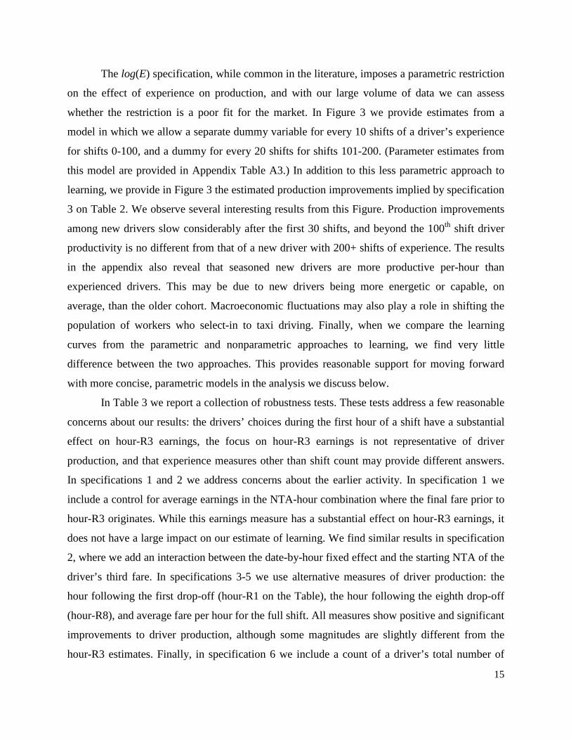
The log(E) specification, while common in the literature, imposes a parametric restriction

on the effect of experience on production, and with our large volume of data we can assess

whether the restriction is a poor fit for the market. In Figure 3 we provide estimates from a

model in which we allow a separate dummy variable for every 10 shifts of a driver’s experience

for shifts 0-100, and a dummy for every 20 shifts for shifts 101-200. (Parameter estimates from

this model are provided in Appendix Table A3.) In addition to this less parametric approach to

learning, we provide in Figure 3 the estimated production improvements implied by specification

3 on Table 2. We observe several interesting results from this Figure. Production improvements

among new drivers slow considerably after the first 30 shifts, and beyond the 100th shift driver

productivity is no different from that of a new driver with 200+ shifts of experience. The results

in the appendix also reveal that seasoned new drivers are more productive per-hour than

experienced drivers. This may be due to new drivers being more energetic or capable, on

average, than the older cohort. Macroeconomic fluctuations may also play a role in shifting the

population of workers who select-in to taxi driving. Finally, when we compare the learning

curves from the parametric and nonparametric approaches to learning, we find very little

difference between the two approaches. This provides reasonable support for moving forward

with more concise, parametric models in the analysis we discuss below.

In Table 3 we report a collection of robustness tests. These tests address a few reasonable

concerns about our results: the drivers’ choices during the first hour of a shift have a substantial

effect on hour-R3 earnings, the focus on hour-R3 earnings is not representative of driver

production, and that experience measures other than shift count may provide different answers.

In specifications 1 and 2 we address concerns about the earlier activity. In specification 1 we

include a control for average earnings in the NTA-hour combination where the final fare prior to

hour-R3 originates. While this earnings measure has a substantial effect on hour-R3 earnings, it

does not have a large impact on our estimate of learning. We find similar results in specification

2, where we add an interaction between the date-by-hour fixed effect and the starting NTA of the

driver’s third fare. In specifications 3-5 we use alternative measures of driver production: the

hour following the first drop-off (hour-R1 on the Table), the hour following the eighth drop-off

(hour-R8), and average fare per hour for the full shift. All measures show positive and significant

improvements to driver production, although some magnitudes are slightly different from the

hour-R3 estimates. Finally, in specification 6 we include a count of a driver’s total number of

15

prior drop-offs as the measure of experience, and again we find significant evidence of learning.

The magnitude of the learning estimate (0.025) is larger than in our preferred specifications in

Table 2. This parameter estimate may include some upward bias due to reverse causality, as

more productive drivers will be able to generate more drop-offs per shift or hour.

The improvements in driver earnings leave open the question of what drivers might be

doing to improve their outcomes. While we do not directly observe drivers’ choices during a

shift, we track how several production outcomes vary with experience. These outcomes, which

we described above, are considered in Table 4. Specifications 1 and 2 track improvements in a

critical driver activity: reducing the amount of time between customers. Specification 1, in which

we consider the share of hour-R3 without passengers, shows that new drivers start with a

significantly larger fraction of hour-R3 idle, and then significantly improve in this outcome with

experience. Likewise, the logged slack time between the driver’s third drop-off and his next

customer (i.e., the first fare of hour-R3) is significantly greater for new drivers, but this falls

steadily with experience. Given these results, it is sensible that more experienced drivers are

observed to transport passengers a greater number of miles (specification 3). We find that new

drivers have lower-mileage trips, on average, which may be due to the types of neighborhoods in

which they search for customers. One possible explanation for improvements in drivers’ earnings

is faster travel while passengers are in the car, and an initial examination of the data in

specification 5 shows that this may be true: brand new drivers appear to travel about 9% slower

than experienced drivers. Speed differences between new and experienced drivers fall somewhat

once we add a control for the driver’s average miles per ride (which could be influenced by

longer trips on higher-speed roads), but significant differences remain. While we do not have

direct evidence on drivers’ decisions to avoid congestion or construction, the results of

specification 6 suggest that experienced drivers may navigate NYC streets more efficiently than

new drivers.

4.2 Productivity, learning, and task difficulty

One strength of our data is that we can examine how new drivers’ production lags behind

experienced drivers’ across a variety of situations, and also how new drivers make progress in

different settings. For this analysis, we separate the city’s NTA-hour (of week) combinations into

quartiles by the average earnings of drivers in the 60 minutes following a drop-off. “Difficult”

16

NTA-hour combinations will have relatively low earnings in the hour following a drop-off.

While a separate difficulty statistic can be calculated for each NTA-hour combination, the

distribution of drop-offs across these is far from uniform (i.e. midtown Manhattan drop-offs are

substantially more common than Staten Island). To address this issue, we construct the quartiles

at the level of the (full) fare data rather than the NTA-hour combination. While the full data have

observations split into equal fourths before we apply the sample restrictions and cleaning steps

described above in Section 3, the analysis sample departs from this weighting somewhat.

We estimate a regression model that allows new drivers to have different expected

earnings at the start of their career in each difficulty quartile, experience different rates of

improvement in each quartile, and allows experienced drivers to vary in their average earnings

across difficulty quartiles as well. The base model is:

log(hour-R3 fare𝑖𝑡) = ��1{𝑄𝑖𝑡 = 𝑞} × 1{𝑖 new} × �θ0𝑞 + θ1𝑞 log(𝐸𝑖𝑡)��4

𝑞=1

+ � 1{𝑄𝑖𝑡 = 𝑞}3

𝑞=1

µ𝑞 + 𝑋𝑖𝑡β + αℎ + ε𝑖𝑡.

The variable Qit contains the difficulty quartile (q) in which driver i drops-off his third customer,

starting hour-R3. 1{.} is the indicator function. New drivers have a different intercept (θ0q) and

learning coefficient (θ1q) for each possible difficulty quartile. These parameters capture,

respectively, the productivity lag of brand new drivers across different quartiles and the rate at

which new drivers’ production improves across quartiles as they accumulate experience (E).

Experienced drivers in the bottom three quartiles have earnings that differ by µq from the

(excluded) earnings of experienced drivers in the easiest quartile. The control variables (X),

market condition fixed effects (α), and error term (ε) are all defined as in the models discussed

above.

We report the results of this analysis in Table 5. In specification 1 we specify αh to

include date-by-hour fixed effects to control for market conditions. We find that driver

productivity, as measured through hour-R3 earnings, is 14% lower for brand new drivers

operating in the most difficult quartile than it is for experienced drivers in the same quartile.

Experienced drivers in the most difficult quartile, in turn, have earnings that are 26% below

those of experienced drivers in the easiest quartile. Note that this difference within experienced

17

drivers is substantially larger than difference between new and experienced drivers in overall

earnings reported on Table 2’s preferred specification 3. New drivers in the middle two quartiles

start their driving careers 10% and 8% below the productivity of experienced drivers, while

drivers in the easiest quartile are just 1.5% below experienced drivers. While new drivers

perform substantially worse than experienced drivers in difficult situations, their performance

improves in these settings more quickly than in the three easier quartiles. In fact, the more

difficult a quartile is for new drivers, the faster earnings improve.

One possible concern about this analysis is that savvy drivers will make choices within

their first three fares that reduce the chance of starting hour-R3 in a difficult location. If drivers

are non-randomly assigned to neighborhoods, then part of the earnings penalty of a difficult

neighborhood will be due to below-average drivers sorting into those areas. We address this

concern by adding to X the logged average earnings of the NTA of the driver’s third pick-up

location. This variable accounts for the final choice the driver could make before hour-R3, and

drivers who find better neighborhoods will be distinguished by picking up their last passengers in

high-earning areas. In specification 2 of Table 5 we find that hour-R3 earnings are increasing in

the value of the third fare’s pick-up location, as expected, but very little changes in the way in

which brand new drivers lag experienced ones or the way in which the new drivers’ earnings

improve with experience. This provides some evidence in favor of our assumption that drop-off

locations, conditional on pick-up locations, are a credible randomizing device for selecting the

neighborhoods reached by drivers. We extend our analysis in specification 3, where we replace

the control variable for third-fare pick-up earnings with a separate neighborhood fixed effect

which is fully interacted with our date-by-hour fixed effects. This allows different neighborhoods

to vary in the magnitude in which their expected earnings carry-over to driver activity in the

following hour. Again we find very little movement in the estimated parameters. New drivers lag

experienced drivers by substantially more in difficult settings, but new drivers also improve

relatively quickly in these settings. The coefficient estimates of specification 3 imply that new

drivers in hardest-quartile (Q1) situations require 136 shifts to eliminate the productivity

difference between themselves and experienced drivers; in the second-easiest quartile (Q3)

drivers require 78 shifts.8

8 For new drivers in Q1 situations, we solve -0.137 + 0.0279×log(t’) = 0 for t’ to obtain the number of shifts until convergence for new and experienced drivers’ expected hour-R3 earnings.

18

4.3 General and specific experience

Our final set of analyses employs separate measures of driver experience across locations and

location-time combinations. While there exists a substantial literature on general versus specific

human capital, which we describe briefly in the Introduction, to our knowledge this literature

relies on relatively small datasets, fairly coarse measures of specific experience, and difficult-to-

evaluate or -test identification arguments. (Consider the example of workers who are switched

between jobs, and the potential questions about which workers are selected for switching.) By

contrast, we have the randomizing device of customers asking for drop-offs in a variety of

neighborhoods, which themselves vary in their earning opportunities and (perhaps) optimal

strategies for finding customers.

We employ several measures of specific experience, and we contrast these with “general”

experience as measured through a driver’s cumulative number of drop-offs. These experience

measures are tied to the location and (in some cases) time of the drop-off for a new driver’s third

customer in shift t. As of this drop-off, the driver is observed to have accumulated dt total drop-

offs through the present customer, with dlt drop-offs in the same location l (PUMA or NTA) as

the customer. In addition, we divide the day into six time blocks (b) which run 11pm-5am, 5am-

11am, 11am-5pm, and 5pm-11pm, and we compute the driver’s cumulative number of drop-offs

that occur through shift t in location l during block b: dlbt. We intend the blocks to capture

different neighborhood-specific patterns in demand that correspond to different times of day. We

utilize these drop-off counts by calculating the share, slt = dlt/dt, that has occurred in location l

through shift t; we also calculate the share that has occurred in the same location and time block,

slbt = dlbt/dt. Finally, to limit colinearity concerns, we construct the share of total activity that

occurs within a PUMA or NTA but outside of the current time block. Among new drivers, the

mean value of slt is 17% for the hour-R3 PUMA, and 8% for the hour-R3 NTA. Within a portion

of the day, the mean values of slbt are 8% for PUMAs and 4% for NTAs. (The shares of within-

location activity outside of the current time block are roughly the same respective magnitudes,

due to the common practice of twelve-hour shifts for drivers.) We consider the impact of these

experience measures by gradually layering them into models of driver earnings during hour-R3.

In all models we interact date-by-hour fixed effects with an additional set of indicators for the

pick-up location of the driver’s third fare. To account for the possibility that drivers accumulate

19

less experience in neighborhoods that are more difficult, we include the log of mean earnings for

the NTA-hour of ride 3’s drop-off.

We report in Table 6 our results on general and specific experience. Our first

specification is an adaptation of Table 3’s specification 6. In addition to augmenting the prior

model’s fixed effects and controlling for the current NTA-hour’s mean earnings, we add slt at the

PUMA level. The coefficient value on slt implies that moving from the 25th percentile (0.099) of

slt to the 75th percentile (0.255) would provide a 2.7% increase in the expected earnings of a new

driver during hour-R3. We introduce slbt in specification 2 in order to analyze specific experience

at a finer level. We find that time-specific experience has a substantially greater effect on

earnings than experience in the same neighborhood outside of the current time block, although

this latter effect is also significantly positive. Moving from the 25th percentile (0.034) of slbt to

the 75th percentile (0.126) provides a 2.5% increase in hour-R3 earnings, while the same increase

in experience outside of block b in location l provides a 0.6% increase in earnings. Thus, it

appears that specification 1’s result is largely driven by prior experience that occurred in the

same portion of the day as shift t’s third ride. In specifications 3 and 4 we repeat this analysis

while using (tighter) NTA boundaries to define locations; our results are qualitatively similar to

specifications 1 and 2. When we group together all experience within an NTA, we find that our

coefficient estimate (0.148) implies that moving from the 25th percentile (0.032) to the 75th

percentile (0.098) of slt would provide an increase in earnings of 1%. Relative to the PUMA-

level result, the smaller magnitude of the NTA-level result largely is due to the lower shares of

experience drivers have in NTAs compared to PUMAs; the coefficient estimates for the two

geographies are very similar (0.174 for PUMAs and 0.148 for NTAs). As in specification 2, we

find in specification 4 that the benefit from NTA-specific experience is primarily due to

experience in the same time block. Finally, we note that the impact of overall experience (total

drop-offs) is fairly consistent across specifications, and our point estimates are also quite similar

to Table 3’s specification 6, which included no measures of specific experience.

Specifications 1-4 show some decline in the importance of specific experience as we

move from a relative broad geography (PUMAs) to a narrow one (NTA). This suggests a limit to

the value of highly-localized experience for taxi drivers, at least when we measure productivity

through the full hour of fares following shift t’s third ride. We address these ideas in the

remaining specifications of Table 6. First, we examine splitting the driver’s share of experience

20

between the drop-off’s NTA and the portion of the NTA’s PUMA that is outside of the NTA

itself. We report in specification 5 that the share of experience in the surrounding PUMA has a

significantly larger impact on earnings than does the share in the drop-off’s NTA. This may be

due to drivers’ tendencies to search across NTAs following a drop-off, or the sequence of rides

that occur in the full hour following a drop-off. Drivers are more likely to end a ride and start a

subsequent ride in the same PUMA than the same NTA (66% vs. 50%), so PUMA-level

experience may be especially useful for the full hour of customers. In the remaining

specifications of Table 6 we turn to an alternative measure of productivity – slack time following

ride 3 – to confirm our earlier results on specific experience as well as to focus on an outcome

that is more precisely limited to the driver’s circumstances following ride 3. In specification 6 we

report that within-PUMA experience, both inside and outside of the current time block, has a

significant impact on reducing slack time. A new driver at the 75th percentile of slbt will require

about 1 fewer minute to find his next customer than a driver at the 25th percentile of slbt. We

conclude the analysis by repeating specification 5 while using slack time as a measure of driver

productivity. Again we find that experience within a PUMA but outside of the current NTA

matters more than experience in the drop-off’s NTA. Since this dependent variable focuses on

outcomes that immediately follow ride 3, it appears that drivers benefit more from having

experience in the neighborhoods that surround a drop-off than in the drop-off NTA itself.

5. Discussion and conclusions

We have described learning patterns by New York City yellow taxi drivers while controlling for

a wide variety of potential factors that can confound empirical studies of learning by doing. We

find that economically and statistically significant learning occurs among taxi drivers, but these

effects may be overstated in the absence of controls for task selection or time-specific demand

conditions. In addition to studying overall learning, we provide evidence on driver performance

across measurably heterogeneous situations. We find that the performance of new drivers lags

that of experienced drivers by a greater margin in hard situations than easy ones, but

performance gaps are eliminated relatively quickly in hard circumstances. Finally, we document

the importance of specific versus general experience. We find that overall and neighborhood-

specific experience are both important in improvements to driver productivity.

21

We present our results with two main contributions relative to the prior literature. First,

the taxi drivers in our study are able to choose their own production strategies, and through fare-

based compensation they are rewarded directly for strategies that are more successful. This is

novel relative to the manufacturing settings that are commonly studied in the LBD literature,

where workers’ actions may be relatively constrained by production line conventions and rigid

pay practices. Second, the TLC’s fare-level “big data” allow us the opportunity to examine an

unusually large number of economic agents moving though a precisely documented production

environment. The large population of agents allows us benchmark new drivers’ production

relative to experienced drivers’ contemporaneous efforts, which is often impossible in prior

studies that examine single firms or one-time production processes. The location- and time-

specific data on each fare allow us to quantify which production tasks are relatively difficult, as

well as track neighborhood-specific experience to compare with a driver’s total experience in the

market.

Our data and analysis leave open several important questions about learning in general

and performance by NYC taxi drivers specifically. First, we are unable to observe how drivers

may selectively refuse fares to certain neighborhoods, or attempt to charge a price above the

appropriate meter fare. While either type of activity is prohibited by the TLC and can result in

the loss of a hack license, we cannot gauge the frequency of this activity in the market and

whether it is correlated with driver experience. Second, the absence of driver-characteristic data

prevents us from describing which types of drivers learn most quickly, and whether learning is

affected by the driver’s social circle or the organizational arrangements of the medallion owner.

Third, our reduced-form analysis prevents us from studying the precise mechanisms of driver

learning or their welfare benefits. Further work in this area could include descriptions of the

strategies drivers choose for finding new customers, how drivers update their information on

earning opportunities as they gain experience, and the welfare value of improvements to drivers’

information. Finally, additional analysis is needed to assess the validity of our empirical

arguments (on selection, etc.) and results outside of the NYC taxi market.

22

References

Clement, Michael B., Lisa Koonce, and Thomas J. Lopez. 2007. “The Roles of Task-specific Forecasting Experience and Innate Ability in Understanding Analyst Forecasting Performance.” Journal of Accounting and Economics 44 (3): 378–398.

Gathman, Christina and Uta Schonberg. 2010. “How General is Human Capital? A Task-Based Approach.” Journal of Labor Economics 28 (1): 1-49.

Hatch, Nile and David Mowry. 1998. “Process Innovation and Learning by Doing in Semiconductor Manufacturing.” Management Science 44 (11): 1461-1477.

Hendel, Igal and Yossi Spiegel. 2014. “Small Steps for Workers, a Giant Leap for Productivity.” American Economic Journal: Applied Economics 6 (1): 73-90.

Jovanovic, Boyan, and Yaw Nyarko. 1995. “A Bayesian Learning Model Fitted to a Variety of Empirical Learning Curves.” Brookings Papers on Economic Activity. Microeconomics 1995: 247-305.

Kellogg, R. 2011. “Learning by Drilling: Interfirm Learning and Relationship Persistence in the Texas Oilpatch.” The Quarterly Journal of Economics 126 (4): 1961–2004.

Levitt, Steven D., John List, and Chad Syverson. 2013. “Toward an Understanding of Learning by Doing: Evidence from an Automobile Assembly Plant.” Journal of Political Economy 121 (4): 643–681.

Ost, Ben. 2013. “How Do Teachers Improve? The Relative Importance of Specific and General Human Capital.” American Economic Journal: Applied Economics, forthcoming.

Pisano, GP. 2001. “Organizational Differences in Rates of Learning: Evidence from the Adoption of Minimally Invasive Cardiac Surgery.” Management Science 47 (6): 752–768

Schaller, B. 2006. “The New York City Taxicab Fact Book.” Schaller Consulting, Mars (March).

Schneider, Henry S. 2010. “Moral Hazard in Leasing Contracts: Evidence from the New York City Taxi Industry.” Journal of Law and Economics 53 (4): 783-805.

Shaw, Kathryn and Edward Lazear. 2008. “Tenure and Output.” Labour Economics 15: 710-724.

Rockart, Scott and Nilanjana Dutt. 2013. “The Rate and Potential of Capability Development Trajectories.” Strategic Management Journal, forthcoming.

Thompson, Peter. 2001. “How Much Did the Liberty Shipbuilders Learn? New Evidence for an Old Case Study.” Journal of Political Economy 109 (1): 103–137.

23

———. 2010. “Learning by Doing.” Chapter 11 in the Handbook of Economics of Technical Change, edited by Bronwyn H. Hall and Nathan Rosenberg, North-Holland/Elsevier.

———. 2012. “The Relationship Between Unit Cost and Cumulative Quantity and the Evidence for Organizational Learning-by-Doing.” The Journal of Economic Perspectives 26 (3): 203–224.

24

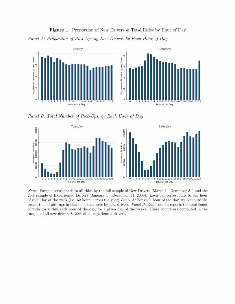
Figure 1: Proportion of New Drivers & Total Rides by Hour of Day

Panel A: Proportion of Pick-Ups by New Driver, by Each Hour of Day0

.1.2

.3.4

Pro

port

ion

of P

ick−

Ups

by

New

Driv

ers

0 1 2 3 4 5 6 7 8 9 10 11 12 13 14 15 16 17 18 19 20 21 22 23Hour of the Day

Tuesday

0.1

.2.3

.4P

ropo

rtio

n of

Pic

k−U

ps b

y N

ew D

river

s

0 1 2 3 4 5 6 7 8 9 10 11 12 13 14 15 16 17 18 19 20 21 22 23Hour of the Day

Saturday

Panel B: Total Number of Pick-Ups, by Each Hour of Day

010

0000

2000

0030

0000

4000

00N

umbe

r of

Pic

k−U

ps

0 1 2 3 4 5 6 7 8 9 10 11 12 13 14 15 16 17 18 19 20 21 22 23Hour of the Day

Tuesday0

1000

0020

0000

3000

00N

umbe

r of

Pic

k−U

ps

0 1 2 3 4 5 6 7 8 9 10 11 12 13 14 15 16 17 18 19 20 21 22 23Hour of the Day

Saturday

Notes : Sample corresponds to all rides by the full sample of New Drivers (March 1 - December 31) and the20% sample of Experienced Drivers (January 1 - December 31, 2009). Each bar corresponds to one hourof each day of the week (i.e. 52 hours across the year) Panel A: For each hour of the day, we compute theproportion of pick-ups in that hour that were by new drivers. Panel B: Each column reports the total countof pick-ups within each hour of the day, for a given day of the week). These counts are computed in thesample of all new drivers & 20% of all experienced drivers.

Figure 2: NTA/DOW/HH-Level Difficulty Measures by Location of Drop-Off

1234No data

Tuesday 8am

1234No data

Tuesday 3pm

1234

Tuesday 10pm

1234No data

Saturday 10pm

Notes : Sample corresponds to 80% of Experienced Drivers (January 1 - December 31, 2009). Difficulty isdefined by a NTA/Day-of-the-Week/Hour-of-the-Day specific measure of the total fare earnings in the 60minutes following a drop-off. This variables is split into quartiles, weighted by the number of rides. Thefourth quartile corresponds to the “easiest” quartile (i.e. highest average fare). 8am corresponds to the hourfalling between 8am and 9am (and similarly for the other reported hours). The maps exclude NTAs 199,299, 399, 498, and 499 which straddle multiple PUMAs (for the empirical analysis, these 5 NTAs are brokeninto 30 distinct NTAs that are nested within PUMAs).

Figure 3: Evaluation of parameteric (log) vs non-parametric (dummy) approaches

−.0

6−

.04

−.0

20

.02

Coe

ffici

ent (

Dep

Var

: Log

(Hou

r−R

3 F

ares

)

*1_10

*11_20

*21_30

*31_40

*41_50

*51_60

*61_70

*71_80

*81_90

*91_100*101_120*121_140*141_160*161_180*181_200

New Driver: # of Shifts Since Starting

Dummies log(E)

Notes : The red line corresponds to Table 2, Specification 3, and uses a natural log specification for g(E)(extrapolating the intercept + log coefficient to shifts 5, 15, 25,...,170,190). The blue line corresponds toAppendix Table 1, Specification 3, and uses a collection of dummy variables for g(E) (minus the coefficienton “Experienced”). “Hour-R3 Fares” is the sum of all fares within the first 60 minutes following the 3rddrop-off of a shift (including fractional fares for those rides that straddle the end of the hour). Samplecorresponds to all rides by the full sample of New Drivers (March 1 - December 31) and the 20% sample ofExperienced Drivers (January 1 - December 31, 2009).

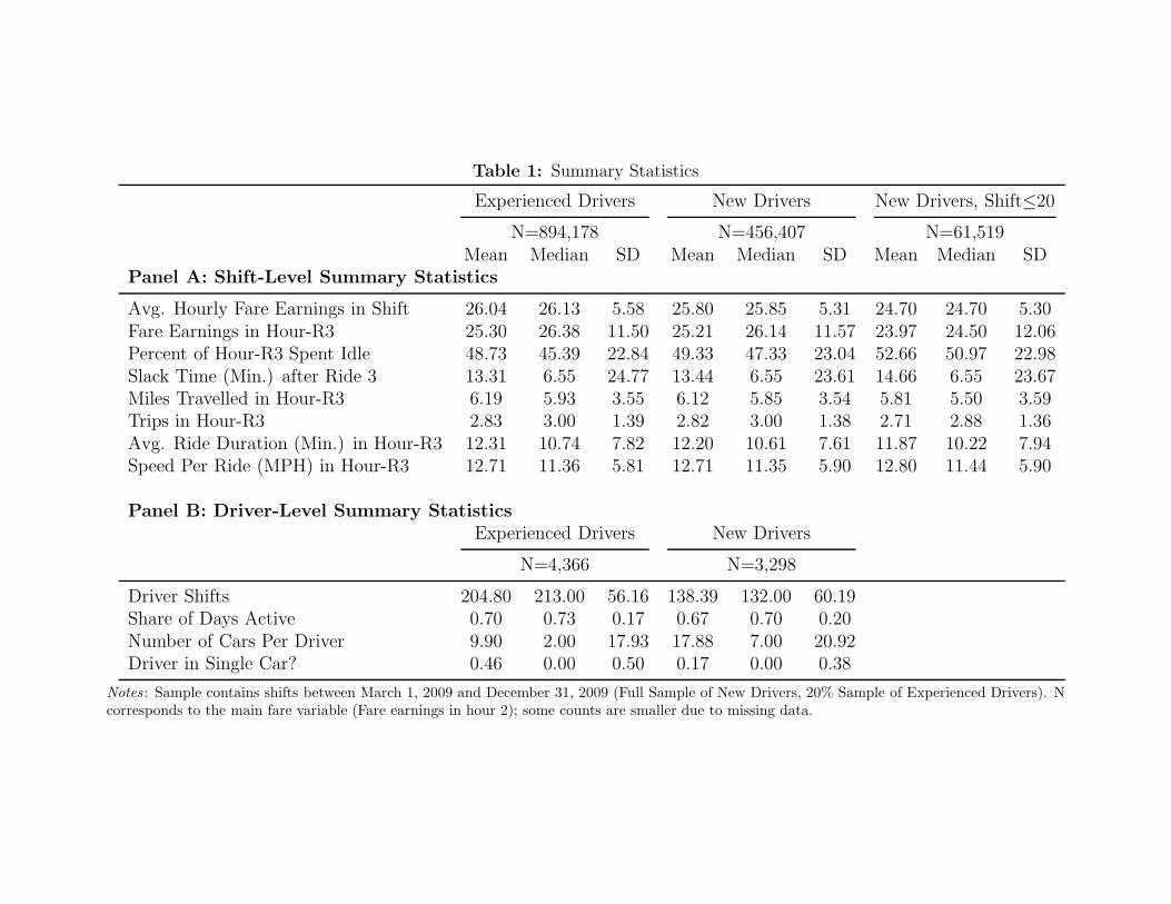
Table 1: Summary Statistics

Experienced Drivers New Drivers New Drivers, Shift≤20

N=894,178 N=456,407 N=61,519Mean Median SD Mean Median SD Mean Median SD

Panel A: Shift-Level Summary Statistics

Avg. Hourly Fare Earnings in Shift 26.04 26.13 5.58 25.80 25.85 5.31 24.70 24.70 5.30Fare Earnings in Hour-R3 25.30 26.38 11.50 25.21 26.14 11.57 23.97 24.50 12.06Percent of Hour-R3 Spent Idle 48.73 45.39 22.84 49.33 47.33 23.04 52.66 50.97 22.98Slack Time (Min.) after Ride 3 13.31 6.55 24.77 13.44 6.55 23.61 14.66 6.55 23.67Miles Travelled in Hour-R3 6.19 5.93 3.55 6.12 5.85 3.54 5.81 5.50 3.59Trips in Hour-R3 2.83 3.00 1.39 2.82 3.00 1.38 2.71 2.88 1.36Avg. Ride Duration (Min.) in Hour-R3 12.31 10.74 7.82 12.20 10.61 7.61 11.87 10.22 7.94Speed Per Ride (MPH) in Hour-R3 12.71 11.36 5.81 12.71 11.35 5.90 12.80 11.44 5.90

Panel B: Driver-Level Summary StatisticsExperienced Drivers New Drivers

N=4,366 N=3,298

Driver Shifts 204.80 213.00 56.16 138.39 132.00 60.19Share of Days Active 0.70 0.73 0.17 0.67 0.70 0.20Number of Cars Per Driver 9.90 2.00 17.93 17.88 7.00 20.92Driver in Single Car? 0.46 0.00 0.50 0.17 0.00 0.38

Notes : Sample contains shifts between March 1, 2009 and December 31, 2009 (Full Sample of New Drivers, 20% Sample of Experienced Drivers). Ncorresponds to the main fare variable (Fare earnings in hour 2); some counts are smaller due to missing data.

Table 2: Driver Experience and Productivity Improvements

Specification: 1 2 3 4Dependent Variable: log(Hour-R3 Fares) log(Hour-R3 Fares) log(Hour-R3 Fares) log(Hour-R3 Fares)Includes Experienced Drivers? N N Y YDriver Fixed Effects?: N N N YTime Fixed Effects: None Date X Hour Date X Hour Date,Hour(no

interaction)

New Driver -0.0811∗∗∗

(0.00536)

New×log(Shift) 0.0361∗∗∗ 0.0269∗∗∗ 0.0187∗∗∗ 0.0160∗∗∗

(0.00158) (0.00198) (0.00123) (0.00110)

N 435,103 435,103 1,281,286 1,281,286r2 0.006 0.201 0.166 0.179∗ p < 0.10, ∗∗ p < 0.05, ∗∗∗ p < 0.01

Notes : Robust standard errors clustered at the driver level, in parentheses. “Hour-R3 Fares” is the sum of all fares within the first 60 minutesfollowing the 3rd drop-off of a shift (including fractional fares for those rides that straddle the end of the hour). Sample contains shifts between March1, 2009 and December 31, 2009 (Full Sample of New Drivers, 20% Sample of Experienced Drivers). All models include controls for the driver’s shiftlength (in hours) and shift length squared.

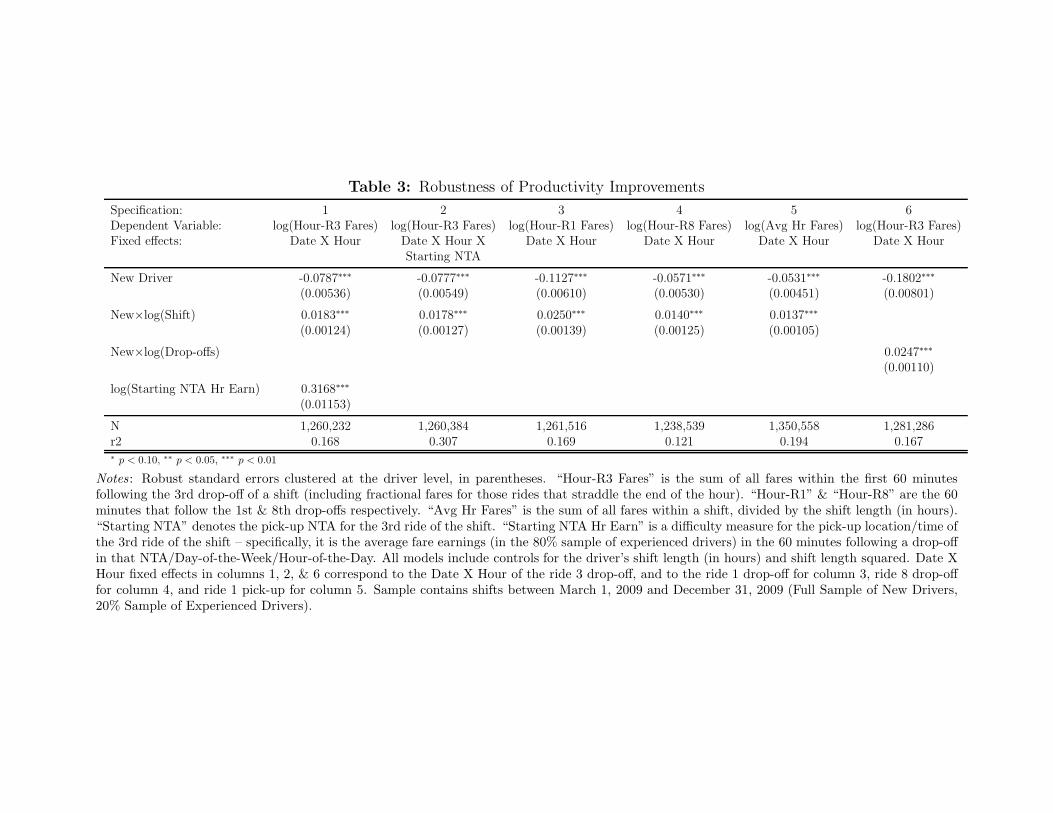
Table 3: Robustness of Productivity Improvements

Specification: 1 2 3 4 5 6Dependent Variable: log(Hour-R3 Fares) log(Hour-R3 Fares) log(Hour-R1 Fares) log(Hour-R8 Fares) log(Avg Hr Fares) log(Hour-R3 Fares)Fixed effects: Date X Hour Date X Hour X Date X Hour Date X Hour Date X Hour Date X Hour

Starting NTA

New Driver -0.0787∗∗∗ -0.0777∗∗∗ -0.1127∗∗∗ -0.0571∗∗∗ -0.0531∗∗∗ -0.1802∗∗∗

(0.00536) (0.00549) (0.00610) (0.00530) (0.00451) (0.00801)

New×log(Shift) 0.0183∗∗∗ 0.0178∗∗∗ 0.0250∗∗∗ 0.0140∗∗∗ 0.0137∗∗∗

(0.00124) (0.00127) (0.00139) (0.00125) (0.00105)

New×log(Drop-offs) 0.0247∗∗∗

(0.00110)

log(Starting NTA Hr Earn) 0.3168∗∗∗

(0.01153)

N 1,260,232 1,260,384 1,261,516 1,238,539 1,350,558 1,281,286r2 0.168 0.307 0.169 0.121 0.194 0.167∗ p < 0.10, ∗∗ p < 0.05, ∗∗∗ p < 0.01

Notes : Robust standard errors clustered at the driver level, in parentheses. “Hour-R3 Fares” is the sum of all fares within the first 60 minutesfollowing the 3rd drop-off of a shift (including fractional fares for those rides that straddle the end of the hour). “Hour-R1” & “Hour-R8” are the 60minutes that follow the 1st & 8th drop-offs respectively. “Avg Hr Fares” is the sum of all fares within a shift, divided by the shift length (in hours).“Starting NTA” denotes the pick-up NTA for the 3rd ride of the shift. “Starting NTA Hr Earn” is a difficulty measure for the pick-up location/time ofthe 3rd ride of the shift – specifically, it is the average fare earnings (in the 80% sample of experienced drivers) in the 60 minutes following a drop-offin that NTA/Day-of-the-Week/Hour-of-the-Day. All models include controls for the driver’s shift length (in hours) and shift length squared. Date XHour fixed effects in columns 1, 2, & 6 correspond to the Date X Hour of the ride 3 drop-off, and to the ride 1 drop-off for column 3, ride 8 drop-offfor column 4, and ride 1 pick-up for column 5. Sample contains shifts between March 1, 2009 and December 31, 2009 (Full Sample of New Drivers,20% Sample of Experienced Drivers).

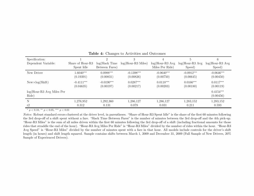
Table 4: Changes to Activities and Outcomes

Specification: 1 2 3 4 5 6Dependent Variable: Share of Hour-R3 log(Slack Time log(Hour-R3 Miles) log(Hour-R3 Avg log(Hour-R3 Avg log(Hour-R3 Avg

Spent Idle Between Fares) Miles Per Ride) Speed) Speed)

New Driver 1.6040∗∗∗ 0.0988∗∗∗ -0.1398∗∗∗ -0.0640∗∗∗ -0.0912∗∗∗ -0.0646∗∗∗

(0.19391) (0.00831) (0.00826) (0.00750) (0.00645) (0.00450)

New×log(Shift) -0.4111∗∗∗ -0.0190∗∗∗ 0.0287∗∗∗ 0.0118∗∗∗ 0.0166∗∗∗ 0.0117∗∗∗

(0.04635) (0.00197) (0.00217) (0.00203) (0.00180) (0.00119)

log(Hour-R3 Avg Miles Per 0.4154∗∗∗

Ride) (0.00456)

N 1,276,952 1,292,360 1,286,127 1,286,127 1,283,152 1,283,152r2 0.312 0.131 0.078 0.031 0.211 0.593∗ p < 0.10, ∗∗ p < 0.05, ∗∗∗ p < 0.01

Notes : Robust standard errors clustered at the driver level, in parentheses. “Share of Hour-R3 Spent Idle” is the share of the first 60 minutes followingthe 3rd drop-off of a shift spent without a fare. “Slack Time Between Fares” is the number of minutes between the 3rd drop-off and the 4th pick-up.“Hour-R3 Miles” is the sum of all miles driven within the first 60 minutes following the 3rd drop-off of a shift (including fractional amounts for thoserides that straddle the end of the hour). “Hour-R3 Avg Miles Per Ride” is “Hour-R3 Miles” divided by the number of rides within the hour. “Hour-R3Avg Speed” is “Hour-R3 Miles” divided by the number of minutes spent with a fare in that hour. All models include controls for the driver’s shiftlength (in hours) and shift length squared. Sample contains shifts between March 1, 2009 and December 31, 2009 (Full Sample of New Drivers, 20%Sample of Experienced Drivers).

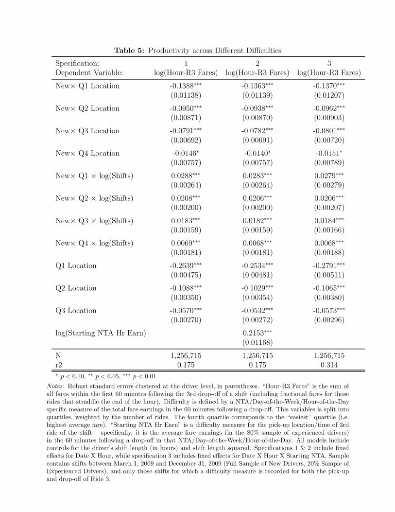
Table 5: Productivity across Different Difficulties

Specification: 1 2 3Dependent Variable: log(Hour-R3 Fares) log(Hour-R3 Fares) log(Hour-R3 Fares)

New× Q1 Location -0.1388∗∗∗ -0.1363∗∗∗ -0.1370∗∗∗

(0.01138) (0.01139) (0.01207)

New× Q2 Location -0.0950∗∗∗ -0.0938∗∗∗ -0.0962∗∗∗

(0.00871) (0.00870) (0.00903)

New× Q3 Location -0.0791∗∗∗ -0.0782∗∗∗ -0.0801∗∗∗

(0.00692) (0.00691) (0.00720)

New× Q4 Location -0.0146∗ -0.0140∗ -0.0151∗

(0.00757) (0.00757) (0.00789)

New× Q1 × log(Shifts) 0.0288∗∗∗ 0.0283∗∗∗ 0.0279∗∗∗

(0.00264) (0.00264) (0.00279)

New× Q2 × log(Shifts) 0.0208∗∗∗ 0.0206∗∗∗ 0.0206∗∗∗

(0.00200) (0.00200) (0.00207)

New× Q3 × log(Shifts) 0.0183∗∗∗ 0.0182∗∗∗ 0.0184∗∗∗

(0.00159) (0.00159) (0.00166)

New× Q4 × log(Shifts) 0.0069∗∗∗ 0.0068∗∗∗ 0.0068∗∗∗

(0.00181) (0.00181) (0.00188)

Q1 Location -0.2639∗∗∗ -0.2534∗∗∗ -0.2791∗∗∗

(0.00475) (0.00481) (0.00511)

Q2 Location -0.1088∗∗∗ -0.1029∗∗∗ -0.1065∗∗∗

(0.00350) (0.00354) (0.00380)

Q3 Location -0.0570∗∗∗ -0.0532∗∗∗ -0.0573∗∗∗

(0.00270) (0.00272) (0.00296)

log(Starting NTA Hr Earn) 0.2153∗∗∗

(0.01168)

N 1,256,715 1,256,715 1,256,715r2 0.175 0.175 0.314∗p < 0.10, ∗∗

p < 0.05, ∗∗∗p < 0.01

Notes : Robust standard errors clustered at the driver level, in parentheses. “Hour-R3 Fares” is the sum ofall fares within the first 60 minutes following the 3rd drop-off of a shift (including fractional fares for thoserides that straddle the end of the hour). Difficulty is defined by a NTA/Day-of-the-Week/Hour-of-the-Dayspecific measure of the total fare earnings in the 60 minutes following a drop-off. This variables is split intoquartiles, weighted by the number of rides. The fourth quartile corresponds to the “easiest” quartile (i.e.highest average fare). “Starting NTA Hr Earn” is a difficulty measure for the pick-up location/time of 3rdride of the shift – specifically, it is the average fare earnings (in the 80% sample of experienced drivers)in the 60 minutes following a drop-off in that NTA/Day-of-the-Week/Hour-of-the-Day. All models includecontrols for the driver’s shift length (in hours) and shift length squared. Specifications 1 & 2 include fixedeffects for Date X Hour, while specification 3 includes fixed effects for Date X Hour X Starting NTA. Samplecontains shifts between March 1, 2009 and December 31, 2009 (Full Sample of New Drivers, 20% Sample ofExperienced Drivers), and only those shifts for which a difficulty measure is recorded for both the pick-upand drop-off of Ride 3.

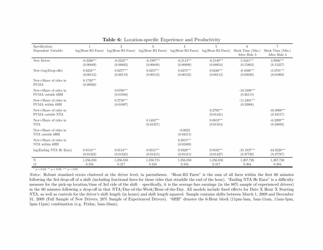
Table 6: Location-specific Experience and Productivity

Specification: 1 2 3 4 5 6 7Dependent Variable: log(Hour-R3 Fares) log(Hour-R3 Fares) log(Hour-R3 Fares) log(Hour-R3 Fares) log(Hour-R3 Fares) Slack Time (Min.) Slack Time (Min.)

After Ride 3 After Ride 3

New Driver -0.2200∗∗∗ -0.2323∗∗∗ -0.1997∗∗∗ -0.2113∗∗∗ -0.2140∗∗∗ 5.3441∗∗∗ 4.9936∗∗∗

(0.00849) (0.00882) (0.00849) (0.00899) (0.00854) (0.15803) (0.15257)

New×log(Drop-offs) 0.0258∗∗∗ 0.0277∗∗∗ 0.0257∗∗∗ 0.0275∗∗∗ 0.0246∗∗∗ -0.4506∗∗∗ -0.3781∗∗∗

(0.00112) (0.00119) (0.00113) (0.00122) (0.00113) (0.02030) (0.01969)

New×Share of rides in 0.1739∗∗∗

PUMA (0.00920)

New×Share of rides in 0.0700∗∗∗ -10.5398∗∗∗

PUMA outside 6HH (0.01948) (0.36114)

New×Share of rides in 0.2738∗∗∗ -11.2401∗∗∗

PUMA within 6HH (0.01697) (0.33908)

New×Share of rides in 0.2793∗∗∗ -16.3009∗∗∗

PUMA outside NTA (0.01431) (0.34517)

New×Share of rides in 0.1482∗∗∗ 0.0853∗∗∗ -6.3399∗∗∗

NTA (0.01357) (0.01354) (0.29893)

New×Share of rides in -0.0022NTA outside 6HH (0.03214)

New×Share of rides in 0.2615∗∗∗

NTA within 6HH (0.02489)

log(Ending NTA Hr Earn) 0.9154∗∗∗ 0.9154∗∗∗ 0.9315∗∗∗ 0.9320∗∗∗ 0.9102∗∗∗ -35.1837∗∗∗ -34.9228∗∗∗

(0.01423) (0.01423) (0.01415) (0.01415) (0.01427) (0.37720) (0.37787)

N 1,256,850 1,256,850 1,256,715 1,256,850 1,256,850 1,267,726 1,267,726r2 0.316 0.317 0.316 0.316 0.317 0.304 0.304∗ p < 0.10, ∗∗ p < 0.05, ∗∗∗ p < 0.01

Notes : Robust standard errors clustered at the driver level, in parentheses. “Hour-R3 Fares” is the sum of all fares within the first 60 minutesfollowing the 3rd drop-off of a shift (including fractional fares for those rides that straddle the end of the hour). “Ending NTA Hr Earn” is a difficultymeasure for the pick-up location/time of 3rd ride of the shift – specifically, it is the average fare earnings (in the 80% sample of experienced drivers)in the 60 minutes following a drop-off in that NTA/Day-of-the-Week/Hour-of-the-Day. All models include fixed effects for Date X Hour X StartingNTA, as well as controls for the driver’s shift length (in hours) and shift length squared. Sample contains shifts between March 1, 2009 and December31, 2009 (Full Sample of New Drivers, 20% Sample of Experienced Drivers). “6HH” denotes the 6-Hour block (11pm-5am, 5am-11am, 11am-5pm,5pm-11pm) combination (e.g. Friday, 5am-10am).

A Appendix

Table A.1: Tests of Randomization Assumption (Transition between Pick-Up & Drop-Off)Specification: 1 2 3 4 5 6Dependent Variable: NTA/DOW/HH Difficulty for Drop-off (Ride 3) PUMA/DOW/HH Difficulty for Drop-off (Ride 3)

Mean Mean Mean Log(Mean) Mean Log(Mean)

Fixed effects: None Date X Hour Date X Hour X Date X Hour X Date X Hour X Date X Hour XStarting NTA Starting NTA Starting NTA Starting NTA

New Driver -0.8811∗∗∗ -0.0507∗∗∗ 0.0045 0.0002 -0.0043 0.0002(0.08676) (0.01193) (0.01041) (0.00042) (0.01009) (0.00042)

New×log(Shift) 0.1732∗∗∗ 0.0103∗∗∗ -0.0014 -0.0001 -0.0003 -0.0001(0.01975) (0.00284) (0.00244) (0.00010) (0.00235) (0.00010)

Constant 26.9845∗∗∗ 26.9301∗∗∗ 26.9276∗∗∗ 3.2831∗∗∗ 26.7856∗∗∗ 3.2831∗∗∗

(0.03664) (0.00279) (0.00182) (0.00007) (0.00197) (0.00007)

N 1,320,911 1,320,911 1,320,911 1,320,911 1,325,465 1,321,066r2 0.001 0.831 0.876 0.874 0.895 0.874∗ p < 0.10, ∗∗ p < 0.05, ∗∗∗ p < 0.01

Notes : Robust standard errors clustered at the driver level, in parentheses. Sample contains shifts betweenMarch 1, 2009 and December 31, 2009 (Full Sample of New Drivers, 20% Sample of Experienced Drivers),and only those shifts for which a difficulty measure is recorded for both the pick-up and drop-off of Ride 3.

Table A.2: Baseline Analysis with Alternative Driver Samples

Specification: 1 2 3 4Dependent Variable: log(Hour-R3 Fares) log(Hour-R3 Fares) log(Hour-R3 Fares) log(Hour-R3 Fares)Includes Experienced Drivers? N N Y YDriver Fixed Effects?: N N N YTime Fixed Effects: None Date X Hour Date X Hour Date,Hour(no

interaction)Panel A: Sample: Drivers Observed in Every Month (Mar-Dec)

New Driver -0.0512∗∗∗

(0.01037)

New×log(Shift) 0.0279∗∗∗ 0.0327∗∗∗ 0.0126∗∗∗ 0.0134∗∗∗

(0.00302) (0.00953) (0.00216) (0.00203)

N 108,919 108,919 792,321 792,321r2 0.004 0.239 0.161 0.173

Panel B: Sample: Drivers Observed in Every Month After Entry

New Driver -0.0968∗∗∗

(0.00625)

New×log(Shift) 0.0416∗∗∗ 0.0283∗∗∗ 0.0213∗∗∗ 0.0188∗∗∗

(0.00185) (0.00233) (0.00143) (0.00130)

N 320,476 320,476 1,017,913 1,017,913r2 0.007 0.209 0.168 0.177∗ p < 0.10, ∗∗ p < 0.05, ∗∗∗ p < 0.01

Notes : Robust standard errors clustered at the driver level, in parentheses. “Hour-R3 Fares” is the sum ofall fares within the first 60 minutes following the 3rd drop-off of a shift (including fractional fares for thoserides that straddle the end of the hour). All models include controls for the driver’s shift length (in hours)and shift length squared. Sample contains shifts between March 1, 2009 and December 31, 2009 (Full Sampleof New Drivers, 20% Sample of Experienced Drivers).

Table A.3: Non-parametric Approach to Driver Experience

Specification: 1 2 3Dependent Variable: log(Hour-R3 Fares) log(Hour-R3 Fares) log(Hour-R3 Fares)Includes Experienced Drivers? N N YIncluded fixed effects: None Date X Hour Date X Hour

New×Shift 1-10 -0.1398∗∗∗ -0.1025∗∗∗ -0.0733∗∗∗

(0.00889) (0.00929) (0.00659)

New×Shift 11-20 -0.1031∗∗∗ -0.0740∗∗∗ -0.0474∗∗∗

(0.00863) (0.00858) (0.00629)

New×Shift 21-30 -0.0900∗∗∗ -0.0662∗∗∗ -0.0435∗∗∗

(0.00863) (0.00824) (0.00630)

New×Shift 31-40 -0.0736∗∗∗ -0.0520∗∗∗ -0.0327∗∗∗

(0.00853) (0.00783) (0.00615)

New×Shift 41-50 -0.0679∗∗∗ -0.0473∗∗∗ -0.0307∗∗∗

(0.00851) (0.00753) (0.00607)

New×Shift 51-60 -0.0658∗∗∗ -0.0415∗∗∗ -0.0281∗∗∗

(0.00852) (0.00731) (0.00606)

New×Shift 61-70 -0.0623∗∗∗ -0.0393∗∗∗ -0.0264∗∗∗

(0.00853) (0.00725) (0.00614)

New×Shift 71-80 -0.0615∗∗∗ -0.0345∗∗∗ -0.0236∗∗∗

(0.00859) (0.00712) (0.00614)

New×Shift 81-90 -0.0572∗∗∗ -0.0273∗∗∗ -0.0171∗∗∗

(0.00848) (0.00690) (0.00602)

New×Shift 91-100 -0.0432∗∗∗ -0.0173∗∗ -0.0082(0.00859) (0.00686) (0.00612)

New×Shift 101-120 -0.0413∗∗∗ -0.0177∗∗∗ -0.0104∗

(0.00815) (0.00630) (0.00565)

New×Shift 121-140 -0.0317∗∗∗ -0.0153∗∗ -0.0092(0.00832) (0.00611) (0.00565)

New×Shift 141-160 -0.0141∗ -0.0116∗∗ -0.0071(0.00823) (0.00593) (0.00559)

New×Shift 161-180 -0.0018 -0.0120∗∗ -0.0092∗

(0.00787) (0.00562) (0.00542)

New×Shift 181-200 0.0123 -0.0046 -0.0033(0.00750) (0.00583) (0.00569)

Experienced -0.0202∗∗∗

(0.00587)

N 435,103 435,103 1,281,286r2 0.006 0.201 0.166∗p < 0.10, ∗∗

p < 0.05, ∗∗∗p < 0.01

Notes : Robust standard errors clustered at the driver level, in parentheses. “Hour-R3 Fares” is the sum ofall fares within the first 60 minutes following the 3rd drop-off of a shift (including fractional fares for thoserides that straddle the end of the hour). All models include controls for the driver’s shift length (in hours)and shift length squared. Sample contains shifts between March 1, 2009 and December 31, 2009 (Full Sampleof New Drivers, 20% Sample of Experienced Drivers).