Learning automata routing in connection-oriented networks

LEARNING AUTOMATA ROUTING

IN CONNECTION-ORIENTED NETWORKS

Anastasios A. Economides

University of MacedoniaThessaloniki 54006, GREECE

Tel # +3031-891799Fax # +3031-891292

[email protected]

20 March 1995

1

Φιλίπ

Text Box

Economides, A.A.: Learning automata routing in connection-oriented networks. International Journal of Communication Systems, Vol. 8, No. 4, pp. 225-237, 1995.

Abstract

Learning automata are used at the source nodes of a connection-

oriented network to dynamically route newly arriving virtual calls to

their destination.

First, two new learning automata are introduced. Then, these two

learning automata, as well as the well-known L learning automaton

and the deterministic shortest-path algorithms are used in a simula-

tion program to route virtual calls. The more frequent the updating

and the more recent network state information used, the better the

performance.

In the sequence, the virtual link length is developed as a function

of both the number of packets and the number of virtual calls at the

network link. This virtual link length is used in the learning automata

routing algorithm and is showed via simulation to be superior to the

minimum packet delay or shortest-queue-type link length, usually used

in real networks. Thus, in connection-oriented networks, not only the

packet but also the virtual call traffic characteristics should be used

in the routing decisions.

Furthermore, when the network state information is out-of-date,

or when there are few virtual calls and each one carries a large number

of packets, then the virtual link length should be based more on the

number of virtual calls than on the number of packets at this link.

On the other hand, when the network state information is current

and there are many virtual calls and each one carries a small number

of packets, then the virtual link length should be based more on the

number of packets than on the number of virtual calls at this link.

Key-words: connection-oriented networks, learning automata routing, simu-lation, virtual calls, virtual circuit networks.

2

1 INTRODUCTION

Dynamic routing in connection-oriented or virtual circuit networks is theselection for every newly arriving virtual call of the currently best path fromits source to its destination node. Dynamic routing may be implementedaccording to two ways:

1) In deterministic routing, the selection of a route from source to des-tination is done deterministically. If our network model is correct and thenetwork state does not change drastically from the moment we measure ituntil we make the routing decisions, then we may act with confidence (ina deterministic way) that our routing decisions are correct. One possiblerule to achieve the optimal routing is with a weighted round-robin fashion.Another possible rule is to select a route if the cost of this route is less thanthe cost of all other possible routes.

2) In probabilistic routing, the selection of a route from source to desti-nation, is done probabilistically. Note, that deterministic routing is a specialcase of probabilistic routing (with probability 1). Solving the routing problemin computer networks, we only find (if we can) the ”solution” to an approx-imation of the real problem. The underlying assumptions of the model (e.g.independent exponential distributions), or even other management problemsthat are not explicitly considered, affect the ”solution”. Thus, instead ofusing a definitive decision (by completely trusting the optimality conditionsand the measurements) a probabilistic one may be used favoring some action.

In this paper, we propose such a probabilistic routing approach basedon learning automata algorithms. These are adaptive control algorithmsfor highly uncertain systems [20]. They select probabilistically an actionand then update their action probabilities according to the outcome of theselected action. If the outcome is favorable, then the probability of the se-lected action increases, otherwise it decreases. So, instead of deterministicallychoosing an action, learning automata choose it with very high probability.Note, that if we appropriatelly calibrate the step size of these learning au-tomata algorithms, then they may choose an action deterministically (withprobability 1).

The greatest potential of the learning automata methodology is that itpermits the control of very complex dynamic systems. Even when littleinformation is available, they act to minimize the effects of future systemchanges. Learning automata have been applied to routing problems like

3

telephone routing [1, 21, 22, 24, 28, 29], datagram routing [5, 11, 14, 15,18, 26, 27], and virtual circuit routing [10, 8]. British Telecom has alreadydeveloped a learning automata routing system for use in their long distancenetwork [4].

Glorioso, Grueneich & Dunn [14] use learning automata for routing. Ifa call is successful through a path, the probability of using the same pathis increased, otherwise it is decreased. Simulation results show the abilityof learning automata to route the traffic around the destroyed portions ofthe network and provide an improved grade of service. Glorioso, Grueneich& McElroy [15] equalize the loading on the network links using learningautomata routing. They demonstrate the ability of learning automata toadapt to a loss of network facilities and to operate with uncertain networkfacilities.

Narendra, Wright & Mason [24] use the M automaton for telephone callrouting. An action corresponds to a sequence of alternate paths to be at-tempted. The penalty probability of each action is updated according tothe success or blocking of the telephone call. At overload conditions, learn-ing automata routing results in a lower blocking probability and lower nodecongestion compared to fixed rule alternate routing.

Narendra & Thathachar [22] introduce two new models of nonstationaryrandom environments. When an action is performed, its penalty probabilityincreases while the penalty probabilities of the other actions decrease. Theyprove that the LR−P automaton operating in such environment tends toequalize the expected penalty probabilities. Simulation of telephone callrouting confirms the equalization of the blocking probabilities.

Chrystall & Mars [5] route messages over the outgoing links using learningautomata at every network node. The delay experienced by every message isused to update the probability of selecting the same link again. They pointout that the LR−I automaton attempts to equalize the average path delays,while the LR−P automaton attempts to equalize the accumulated path delays.

Srikantakumar & Narendra [28] analyze nonstationary environments wherethe penalty probabilities are functions of the action probabilities. They provethat the LR−P automaton equalizes the penalty rates, while the LR−εP au-tomaton equalizes the penalty probabilities. For telephone call routing, theLR−P automaton attempts to equalize the rates of the call blocking proba-bilities, while the LR−εP automaton attempts to equalize the call blockingprobabilities. Further simulation results by Narendra & Mars [21] verify the

4

behavior predicted by the theoretical analysis.Mason [18] proposes new learning automata algorithms to route packets

in packet switched networks. The routing parameters are updated accordingto the packet delays on the links. Simulation results show the superiority ofthe learning automata routing over fixed and random routing.

Akselrod and Langholz [1] show via simulation that learning automatarouting performs better than fixed routing for telephone networks. Further-more, they introduce a penalty function of the number of calls on each trunkgroup to represent its load.

Nedzelnitsky and Narendra [26] propose a new model for nonstation-ary enironments whose penalty probabilities depend on the previous penaltyprobabilities and on the probabilities of the performed actions. Then theysimulate routing in datagram packet switched network by learning automataat every network node. The SLR−I and SLR−εP automata equalize the de-lays, while the SLR−P automaton equalizes the delay rates.

Zgierski & Oommen [29] show via object-oriented simulation the superi-ority of learning automata telephone call routing to fixed rule and randomrouting in terms of call blocking probability. Their simulation environmentuses any of the M-automaton, several linear learning automata, the corre-sponding discrete learning automata and their absorbing versions.

Economides & Silvester [11] propose learning automata for routing pack-ets in a network with unreliable links. The routing probabilities are updatedaccording to the success or failure of packet transmission, or according to themarginal packet delays over the unreliable links. Learning automata are alsoused to estimate the link error rates.

Economides, Ioannou & Silvester [10] propose learning automata for rout-ing virtual calls. The routing probabilities are updated according to theunfinished work on the paths. Simulation results show equalization of theunfinished work on the paths. Furthermore, two other extensions on thelearning automata updating algorithms are proposed: the multiple responselearning automata (which are analyzed mathematically in [9]), and the vir-tual updating learning automata.

In this paper, we extend our results on introducing learning automata[10] at the source nodes of the network to dynamically route newly arrivingvirtual calls to their destination. In section 2, we introduce two new learn-ing automata and propose the learning automata routing of virtual calls inconnection-oriented networks. In section 3, we simulate virtual circuit net-

5

works and use the two new learning automata, as well as the L learningautomaton and the deterministic algorithm for routing newly arriving vir-tual calls. We find that the more frequent the updating and the more recentinformation used, the better the performance.

In section 4, we develop a new measure of the link load, the virtual linklength, which is a function of both the number of packets and the numberof virtual calls at this link. We use it to update the learning automatonrouting algorithm, that probabilistically routes every newly arriving virtualcall. We show via simulation that this virtual link length is superior to theminimum packet delay or shortest-queue-type link length, usually used in realnetworks [2, 3, 12, 13, 16, 17, 19, 25, 30]. Furthermore, when the networkstate information is out-of-date, or when there are few virtual calls and eachone carries a large number of packets, then the number of virtual calls shouldweight more in the virtual link length than the number of packets. On theother hand, when the network state information is current, and there aremany virtual calls and each one carries a small number of packets, then thenumber of packets should weight more in the virtual link length than thenumber of virtual calls. Finally, in section 5, we summarize the results.

2 LEARNING AUTOMATA AS ROUTERS

In this section, we apply three learning automata algorithms to the routingproblem in virtual circuits networks [8]. In these networks, a call set-uppacket, which may be part of the first packet of a message, initiates theestablishment of a virtual circuit from source to destination. All other packetsbelonging to this message follow the same route which remains fixed for theduration of the call [6, 7].

The formulation of the routing problem can be done either on the linkflow space or on the path flow space. In future high speed computer commu-nication networks, the transmission delay will be extremely low and we willnot want to spend extra time in network management decisions inside thenetwork. Therefore, the computationally intensive processes, such as the net-work management decisions, will be transferred outside of the network eitherto the source or to the destination node. With this in mind, we formulatethe routing problem on the path flow space, which means that the controldecisions will be done at the source nodes. In this way, we also avoid loops,

6

since the virtual calls will follow a previously determined loop free path.Since network conditions change very rapidly, the minimum length path

at a time instant may not be the same at the next time instant. Also,the information about the network state is always obsolete and inacurrate.Therefore the routing decisions should not overreact and immediately senda new virtual call along the minimum length path to its destination. Thesystem management decisions should fast track the current network state butwithout introducing instability.

The proposed dynamic virtual call routing algorithms are based on aProbabilistic Selection of the Minimum Length Path idea [10]. Instead ofusing a definitive decision as to where to send a newly arriving virtual call,we vary the routing probabilities favoring the minimum length path.

Every source node [s.] has a learning automaton, for every destinationnode [.d], that routes newly arriving virtual calls at node [s.] and destinedfor node [.d]. These learning automata operate asynchronously and base theirdecisions on the current network state. The actions, a(n), of each automatonare to select some particular path π[sd] to the destination node [.d].

The automaton selects action a(n) = aπ[sd] with probability Pπ[sd](n). Ac-tion a(n) becomes input to the environment. If this results in a favorable out-come for the network performance, then the probability Pπ[sd](n) is increased(rewarded) by ∆Pπ[sd](n) and the Pp[sd](n), ∀p[sd] 6= π[sd], are decreased by∆Pp[sd](n). Otherwise, if an unfavorable outcome happens, then the Pπ[sd](n)is decreased (penalized) by ∆Pπ[sd](n) and the Pp[sd](n), ∀p[sd] 6= π[sd] areincreased by ∆Pp[sd](n).

The simplest information that someone can measure and transfer aboutthe network state is the packet delay through each path from source to des-tination. Measurements of the packet delay are also used in the ARPANETrouting [13, 16, 17, 30] as well as in the Internet routing [19, 25].

In the deterministic shortest-path algorithm, we send a newly arrivingvirtual call along the minimum packet delay path. However, in the threelearning automata algorithms proposed in the next paragraphs, instead ofusing a definitive decision as to where to send a newly arriving virtual call,we vary the path routing probabilities favoring the minimum delay path.Note that the deterministic shortest-path algorithm is a special case of thelearning automata algorithms, since by suitably tuning the parameters, wecan select the minimum length path with probability 1.

The values for the reward and penalty parameters in the learning au-

7

tomata should be chosen by experimentation for specific network topology,number of paths between source-destination pairs, traffic characteristics, in-formation about the network state, updating time interval and other vari-ables. For uniformity across all three learning automata algorithms, wewanted to use the same reward and penalty parameters. After a lengthyexperimentation, we found that the values of reward parameter = 0.2 andpenalty parameter = 0.8 achieve good performance for all three learning au-tomata algorithms. However, as we show in section 3, there exist other valuesfor these parameters in each one of the three learning automata algorithmsthat result in better performance.

2.1 L

The first algorithm uses the well known L learning automaton [23, 20] withreward parameter α = 0.2 and penalty parameter β = 0.8. When an actionis attempted at time n, the L automaton increases at time n+1 the action’sprobability by an amount proportional to one minus its value at n for afavorable response and decreases it by an amount proportional to its valueat n for an unfavorable response. In our case, if the selected path has theminimum packet delay at the next iteration, then we increase the probabilityof selecting it again, otherwise we decrease it. More specifically:

Let path π[sd] is selected for the vth virtual call.

Update the probabilities at time instances n until the (v + 1)th virtual call

arrives:

If Tπ[sd](n) ≤ minp[sd]

{Tp[sd](n)}, then

Pπ[sd](n + 1) = Pπ[sd](n) + 0.2 ∗ [1 − Pπ[sd](n)]Pp[sd](n + 1) = Pp[sd](n) − 0.2 ∗ Pp[sd](n) ∀ p[sd] 6= π[sd]

elsePπ[sd](n + 1) = Pπ[sd](n) − 0.8 ∗ Pπ[sd](n)

Pp[sd](n + 1) = Pp[sd](n) + 0.8 ∗[

1 − Pp[sd](n)]

∀ p[sd] 6= π[sd]

Select the path for the (v + 1)th virtual call probabilistically according to

Pp[sd](v + 1) ∀p[sd].

8

Thus, let path π[sd] is selected for the vth virtual call. Then, we measurethe average packet delay over the selected path π[sd], Tπ[sd], as well as overthe other paths p[sd], Tp[sd], during an updating time interval (n, n+1]. If thedelay over the selected path is less that the delay over the other paths, then weincrease the probability of selecting the same path again, Pπ[sd], and decreasethe probability of selecting any other path, Pp[sd]. Otherwise, if the delay overthe selected path is not the minimum, then we decrease the probability ofselecting the same path again, Pπ[sd], and increase the probability of selectingany other path, Pp[sd]. This updating process is repeated until the nextv + 1 virtual call arrives. At that moment, this new virtual call is routedprobabilistically, according to the current routing probabilities, along a path.

2.2 MRL

The second algorithm uses the S-model Multiple Response Linear (MRL)learning automaton. The norms of behavior for the Q-model MRL learn-ing automaton are investigated in [8, 9]. The idea for the MRL learningautomata is to use different adaptation rates for different environment re-sponses. We consider two response and penalty regions for the algorithmand the functions that define these regions are linear functions with param-eter 2. When the selected path gives very good performance (very smalldelay), then we increase the probability of the selected path very fast. Whenthe selected path gives almost good performance (small delay), then we in-crease the probability of the selected path slowly. Correspondingly, when theselected path gives very bad performance (very large delay), then we decreasethe probability of the selected path very fast. When the selected path givesalmost bad performance (large delay), then we decrease the probability of theselected path slowly. Here, we take as reward parameters α1 = 0.8 (excellentchoice), α2 = 0.2 (good choice, but not excellent) and penalty parametersβ2 = 0.8 (bad choice), β1 = 1 (very bad choice). More specifically:



arrives:

9


{Tp[sd](n)/2}, then


If minp[sd]

{Tp[sd](n)/2} < Tπ[sd](n) ≤ minp[sd]

{Tp[sd](n)},


If minp[sd]

{Tp[sd](n)} ≤ Tπ[sd](n) ≤ minp[sd]

{2 ∗ Tp[sd](n)},

Pπ[sd](n + 1) = Pπ[sd](n) − 0.8 ∗ Pπ[sd](n)

Pp[sd](n + 1) = Pp[sd](n) + 0.8 ∗[

1 − Pp[sd](n)]

∀ p[sd] 6= π[sd]

If minp[sd]

{2 ∗ Tp[sd](n)} ≤ Tπ[sd](n),

Pπ[sd](n + 1) = Pπ[sd](n) − 1 ∗ Pπ[sd](n)

Pp[sd](n + 1) = Pp[sd](n) + 1 ∗[

1 − Pp[sd](n)]

∀ p[sd] 6= π[sd]


Pp[sd](v + 1) ∀p[sd].

The algorithm works as follows: let path π[sd] is selected for the vth

virtual call. Then, we measure the average packet delay over the selectedpath π[sd], Tπ[sd], as well as over the other paths p[sd], Tp[sd], during anupdating time interval (n, n + 1].

If the delay over the selected path is smaller than half of the minimum de-lay over the other paths, then we rapidly increase the probability of selectingthe same path again, Pπ[sd], and rapidly decrease the probability of selectingany other path, Pp[sd]. If the delay over the selected path is larger than halfthe minimum but smaller than the minimum delay over the other paths, thenwe slowly increase the probability of selecting the same path again, Pπ[sd],and slowly decrease the probability of selecting any other path, Pp[sd].

Otherwise, if the delay over the selected path is larger than the minimumbut smaller than double the minimum delay over the other paths, then weslowly decrease the probability of selecting the same path again, Pπ[sd], andslowly increase the probability of selecting any other path, Pp[sd]. If the delay

10

over the selected path is larger than double the minimum delay over the otherpaths, then we rapidly decrease the probability of selecting the same pathagain, Pπ[sd], and rapidly increase the probability of selecting any other path,Pp[sd].

This updating process is repeated until the next v +1 virtual call arrives.At that moment, this new virtual call is routed probabilistically, accordingto the current routing probabilities, along a path.

2.3 SDL

Finally, the third algorithm uses the State Dependent Linear (SDL) learningautomaton [8]. The idea for the SDL learning automaton is to make thereward and penalty parameters functions of the difference of the averagedelay of the selected path and the maximum average delay of the other pathsbetween this source-destination. We use the exponential function in orderto emphasize the difference in the delays. Then, the smaller the delay of apath, the more probable its selection. More specifically:



arrives:


{Tp[sd](n)}, then

Pπ[sd](n + 1) = Pπ[sd](n) + 0.2 ∗ (1 − e[Tπ[sd](n) − max

p[sd]Tp[sd](n)]

) ∗ [1 − Pπ[sd](n)]

Pp[sd](n + 1) = Pp[sd](n) − 0.2 ∗ (1 − e[Tπ[sd](n) − max

p[sd]Tp[sd](n)]

) ∗ Pp[sd](n)∀ p[sd] 6= π[sd]

else

Pπ[sd](n + 1) = Pπ[sd](n) − 0.8 ∗ e[Tπ[sd](n) − max

p[sd]Tp[sd](n)]

∗ Pπ[sd](n)

Pp[sd](n + 1) = Pp[sd](n) + 0.8 ∗ e[Tπ[sd](n) − max

p[sd]Tp[sd](n)]

∗[

1 − Pp[sd](n)]

∀ p[sd] 6= π[sd]


Pp[sd](v + 1) ∀p[sd].

11

So, let path π[sd] is selected for the vth virtual call. Then, we measurethe average packet delay over the selected path π[sd], Tπ[sd], as well as overthe other paths p[sd], Tp[sd], during an updating time interval (n, n + 1].

If the delay over the selected path is smaller than the delay over the otherpaths, then we increase the probability of selecting the same path again,Pπ[sd], and decrease the probability of selecting any other path, Pp[sd]. If thedifference of the delay of the selected path minus the maximum delay overthe other paths, Tπ[sd]− max

p[sd]Tp[sd], is large, this means that the selected path

has very good performance. In this case, the function exp[Tπ[sd]− maxp[sd]

Tp[sd]]

approaches the 0. Therefore, the probability for the selected path, Pπ[sd],increases very fast. If this difference is small, this means that the selectedpath has marginally good performance. In this case, the function exp[Tπ[sd]−maxp[sd]

Tp[sd]] approaches the 1. Therefore, the probability for the selected path,

Pπ[sd], increases slowly. The probabilities for the other paths decrease accord-ingly.

Otherwise, if the delay over the selected path is not the minimum, then wedecrease the probability of selecting the same path again, Pπ[sd], and increasethe probability of selecting any other path, Pp[sd]. If the difference of thedelay over the selected path minus the maximum delay over the other paths,Tπ[sd]− max

p[sd]Tp[sd], is large, this means that the selected path has not so bad

performance. In this case, the function exp[Tπ[sd]− maxp[sd]

Tp[sd]] approaches the

0. Therefore, the probability for the selected path, Pπ[sd], decreases slowly.If this difference is small, this means that the selected path has very poorperformance. In this case, the function exp[Tπ[sd]− max

p[sd]Tp[sd]] approaches the

1. Therefore, the probability for the selected path, Pπ[sd], decreases fast. Theprobabilities for the other paths increase accordingly.

This updating process is repeated until the next v +1 virtual call arrives.At that moment, this new virtual call is routed probabilistically, accordingto the current routing probabilities, along a path.

3 SIMULATION

In this section, we compare the performance of the deterministic shortest-path and the three learning automata algorithms (see previous section) via

12

simulation. In an arbitrary topology network, we consider two specific pathsto be available between a given source-destination pair. We assign a learningautomaton at the source node to route newlly arriving virtual calls througheither the first or the second path. Path # 1 has seven links each one witheffective service rate 1. Path # 2 has seven links with effective service rates1, 0.5, 2, 2, 2, 0.5 and 1. Once a path is selected for a new virtual call,all packets belonging to this virtual call are transmitted through this path.Upon arrival, each packet is sent through the selected path for the virtual callit belongs to. Then the packet is transmitted link-by-link to the destination.

We consider Poisson distributed virtual call arrivals, Poisson distributedpacket arrivals in a virtual call and geometrically distributed number of pack-ets in a virtual call. Then the virtual call duration (lifetime) is exponentiallydistributed. Finally, the packet service requirement is exponentially dis-tributed with mean 1/µ = 1. For the traffic characteristics, we consider twocases:

i) 30/2/40: the mean interarrival time of virtual calls is 1/γ = 30, theinterarrival time of packets in a virtual call is 1/r = 2 and the mean virtualcall duration is 1/δ = 40.

ii) 50/5/200: the mean interarrival time of virtual calls is 1/γ = 50, theinterarrival time of packets in a virtual call is 1/r = 5 and the mean virtualcall duration is 1/δ = 200.

For measuring the path delay and updating the probabilities, we considertwo cases:

i) 1 : at every packet departure from the network through a path, thedestination sends to the source the delay of this last packet through thispath.

ii) 50 : at every 50th packet departure from the network through a path,the destination sends to the source the average packet delay of these 50 lastpackets through this path.

The source node keeps and updates the information about the delay ofits paths to the destination. The information about the delay of a path isupdated every time a packet arrives at the destination through this path.However, this updating is not done immediately, but we assume that thisinformation becomes available to the source node after a feedback delay.We assume that no extra traffic is created for transferring this feedbackinformation to the source node (it is either piggybacked on regular packetsor uses a different channel). We consider two cases for the feedback delay:

13

30/2/40 1 instant 1 obsolete 50 instant 50 obsolete

deterministic 50.59 ±0.89 63.59 ±1.28 55.38 ±0.93 61.97 ±1.36L automaton 50.27 ±1.15 61.29 ±1.36 57.37 ±0.88 61.44 ±1.25MRL automaton 50.64 ±0.73 61.27 ±1.63 61.15 ±0.92 64.04 ±1.36SDL automaton 48.92 ±0.51 62.52 ±1.04 57.37 ±1.14 60.60 ±1.46


deterministic 46.79 ±1.75 57.84 ±1.92 60.52 ±2.21 68.30 ±2.23L automaton 45.35 ±1.45 54.85 ±2.31 61.43 ±1.76 65.43 ±1.77MRL automaton 43.25 ±1.45 56.45 ±2.13 62.05 ±3.16 65.67 ±2.52SDL automaton 46.22 ±1.36 57.45 ±2.17 60.81 ±1.79 67.24 ±1.68

Table 1: The average packet delay ± error (95% confidence interval) fordeterministic, Linear automaton, Multiple Response automaton and StateDependent automaton based routing.

i) instantaneous information, when the feedback delay is 7 time units. Inthis case, we assume that the feedback information has higher priority overother packets and does not wait in queues.

ii) obsolete information, when the feedback delay is 60 time units. Inthis case, we assume that the feedback information is piggybacked on regularpackets and is transferred back to the source node.

Updating the information of a path asynchronously at packet departureinstances has an undesirable characteristic. If a path becomes unattractivefor routing packets through it, then we may not route any more packetsthrough it. However, our information about its length remains the same,although after some time this path may become idle. We have overcome thisproblem by sending a probe packet through a path that has not been usedfor 100 time units. In this way, we may update our information about itsdelay.

In Table 1 and Figures 1-8, we show the simulation results for the averagepacket delay for 10,000 virtual calls.

For given learning parameters α = 0.2 and β = 0.8, all four algorithmsperform similarly, although the learning automata algorithms achieve bet-

14

ter performance. Furthermore, the learning automata have more flexibility,since we can calibrate their learning parameters depending on the particularnetwork topology and traffic characteristics. By suitably tuning the rewardand penalty parameters, the learning automata give improved performance.

For example, in the case of 30/2/40, the L automaton with α = 0 andβ = 0.6 achieves an average packet delay of 45.03 (when 1 instant), 52.42(when 1 obsolete), 54.40 (when 50 instant), 57.99 (when 50 obsolete). Thesedelays are much smaller than those in Table 1.

In the case of 50/5/200, the MRL automaton with [α1 = 0.8, α2 = 1, β2 =1, β1 = 1] achieves an average packet delay of 57.14 (when 50 instant) andwith [α1 = 0.8, α2 = 0.2, β2 = 1, β1 = 1] achieves an average packet delay of64.43 (when 50 obsolete). Again, these delays are much smaller than thosein Table 1.

Another important result is that the more frequent we update the algo-rithms and the more recent network state information we have, the betterthe performance. Thus, the best performance is achieved when the routerknows the delay experienced by every packet as it traverses a particular path,as soon as possible.

4 VIRTUAL LINK LENGTH

In this section, we develop the virtual link length, a new measure for thelink length in virtual circuit networks. We use it in the learning automatarouting algorithm to route newly arriving virtual calls. Then, we show viasimulation its superiority over the minimum packet delay or shortest-queuerouting.

Let a link ij with service rate Cij. We propose as link length lij(n) attime n a convex combination of its current length lcurrent

ij (n) and its expected

length in the future lfutureij (n). In this way, we base our decisions not only on

the current network state, but also on the estimated future network state.We call it virtual link length and define it as [8]:

lij = ε ∗ lcurrentij (n) + (1 − ε) ∗ lfuture

ij (n)

We may consider as current length lcurrentij (n) =

1 + Nij(n)

µCij

, a linear func-

tion of the number of packets on link ij, Nij. This current link length is the

15

estimated packet delay on this link right now. We may consider as future

length lfutureij (n) =

1 + Vij(n)

µCij

, a linear function of the number of virtual calls

on link ij, Vij. This future link length is the estimated packet delay on thislink in the near future.

Then the virtual length of link ij is

lij = ε ∗1 + Nij(n)

µCij

+ (1 − ε) ∗1 + Vij(n)

µCij

0 ≤ ε ≤ 1

A related measure to the virtual link length is the unfinished work [10]:

Uij(n) =1 + Nij(n)

µCij

+r

δ∗

1 + Vij(n)

µCij

where the future link length is weighted by r/δ: the average number ofpackets in a virtual call. The unifinished work represents the average delaydue to both the current packets waiting to be transmitted and the packetsthat are expected to arrive (due to the current open virtual calls) and betransmitted.

The virtual length of a path π[sd] is lπ[sd](n) =∑

ij∈π[sd]

lij(n).

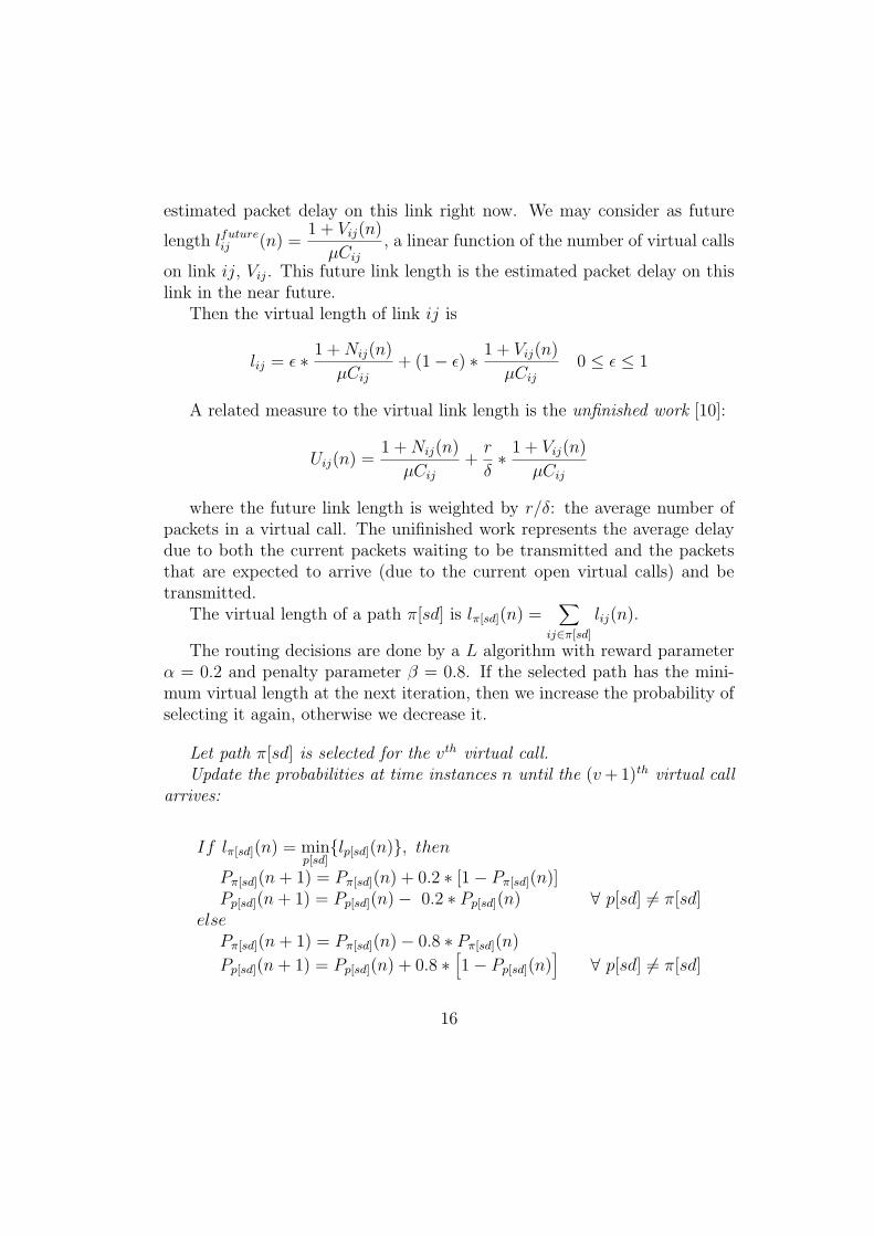
The routing decisions are done by a L algorithm with reward parameterα = 0.2 and penalty parameter β = 0.8. If the selected path has the mini-mum virtual length at the next iteration, then we increase the probability ofselecting it again, otherwise we decrease it.



arrives:

If lπ[sd](n) = minp[sd]

{lp[sd](n)}, then


elsePπ[sd](n + 1) = Pπ[sd](n) − 0.8 ∗ Pπ[sd](n)

Pp[sd](n + 1) = Pp[sd](n) + 0.8 ∗[

1 − Pp[sd](n)]

∀ p[sd] 6= π[sd]

16


Pp[sd](v + 1) ∀p[sd].

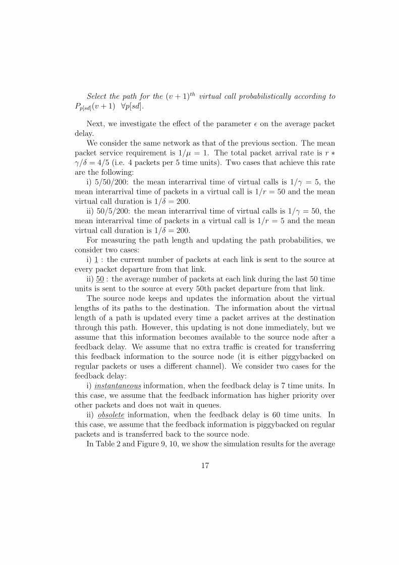
Next, we investigate the effect of the parameter ε on the average packetdelay.

We consider the same network as that of the previous section. The meanpacket service requirement is 1/µ = 1. The total packet arrival rate is r ∗γ/δ = 4/5 (i.e. 4 packets per 5 time units). Two cases that achieve this rateare the following:

i) 5/50/200: the mean interarrival time of virtual calls is 1/γ = 5, themean interarrival time of packets in a virtual call is 1/r = 50 and the meanvirtual call duration is 1/δ = 200.

ii) 50/5/200: the mean interarrival time of virtual calls is 1/γ = 50, themean interarrival time of packets in a virtual call is 1/r = 5 and the meanvirtual call duration is 1/δ = 200.

For measuring the path length and updating the path probabilities, weconsider two cases:

i) 1 : the current number of packets at each link is sent to the source atevery packet departure from that link.

ii) 50 : the average number of packets at each link during the last 50 timeunits is sent to the source at every 50th packet departure from that link.

The source node keeps and updates the information about the virtuallengths of its paths to the destination. The information about the virtuallength of a path is updated every time a packet arrives at the destinationthrough this path. However, this updating is not done immediately, but weassume that this information becomes available to the source node after afeedback delay. We assume that no extra traffic is created for transferringthis feedback information to the source node (it is either piggybacked onregular packets or uses a different channel). We consider two cases for thefeedback delay:

i) instantaneous information, when the feedback delay is 7 time units. Inthis case, we assume that the feedback information has higher priority overother packets and does not wait in queues.

ii) obsolete information, when the feedback delay is 60 time units. Inthis case, we assume that the feedback information is piggybacked on regularpackets and is transferred back to the source node.

In Table 2 and Figure 9, 10, we show the simulation results for the average

17


ε = 0.2 104.22 ±4.50 102.20 ±5.51 133.30 ±5.98 129.71 ±4.92ε = 0.4 59.61 ±3.31 59.97 ±3.06 78.49 ±2.75 73.94 ±2.38ε = 0.6 46.98 ±2.43 46.12 ±1.79 60.88 ±1.67 56.81 ±1.53ε = 0.8 39.77 ±1.05 42.68 ±1.25 64.12 ±2.05 77.94 ±3.33ε = 1 37.19 ±1.22 50.66 ±2.06 104.38 ±4.36 126.66 ±4.45path delay 55.97 ±3.98 97.02 ±8.79 106.41 ±8.03 121.67 ±8.15


ε = 0 73.01 ±3.89 69.24 ±5.15 125.73 ±13.88 100.86 ±7.56ε = 0.2 36.70 ±0.98 37.20 ±0.83 51.43 ±1.66 51.50 ±1.77ε = 0.4 34.39 ±1.05 37.23 ±1.42 64.44 ±1.69 68.90 ±1.71ε = 0.6 34.85 ±1.05 39.41 ±1.10 76.96 ±1.50 85.60 ±1.10ε = 0.8 35.29 ±0.88 41.59 ±1.11 83.39 ±1.19 92.28 ±2.13ε = 1 37.02 ±1.02 44.15 ±0.99 86.26 ±2.34 97.26 ±3.46path delay 45.35 ±1.45 54.85 ±2.31 61.43 ±1.76 65.43 ±1.77

Table 2: The average packet delay ± error (95% confidence interval) fordifferent values of the parameter ε, when we use as path length the sum

of the virtual link lengths lij = ε ∗1 + Nij

µCij

+ (1 − ε) ∗1 + Vij

µCij

, or the path

delay.

packet delay for 10,000 virtual calls.An important observation made in the previous section is also repeated

here: the more frequent we update the learning automaton algorithm and themore recent network state information we have, the better the performance.

We also notice that a proper value for the parameter ε should be exper-imentally selected for best performance. Using only the number of virtualcalls on each link (ε = 0) as the link length is very inefficient (actually, forthe case 5/50/200, the average network delay becomes extremely high andwe do not even show it). Also, it is not always best to use only the numberof packets on each link (ε = 1) as the link length.

For comparison, we also show the average network delay, when we use

18

the packet delay on a path as the path length. We remark that using boththe number of packets and virtual calls is much better than using the packetdelay on the path.

In case, we update the learning automaton infrequently and have obsoletestate information, then it seems better to weight more (ex. ε < 1/2) thenumber of virtual calls, Vij, than the number of packets, Nij, in the virtual

link length. Then, the routing decisions depend more on lfutureij than on

lcurrentij .

When the interarrival time of virtual calls is very short 1/γ = 5, virtualcalls arrive very frequently into the network. On the average, there are γ/δ =40 virtual calls, each one carries r/δ = 4 packets, so there are 160 packetsinto the network. Thus, it is important to weight properly the dependencyof the routing algorithm onto the number of packets and virtual calls. Table2 shows that the routing decisions should be based more on the number ofpackets on each link than on the number of virtual calls on each link. If atevery packet departure, we know the current network state instantaneously,then it is better to base the routing decisions only (100%) on the currentnumber of packets. If at every packet departure, we know the network stateafter a feedback delay, then it is better to base the routing decisions at 80% onthe number of packets and at 20% on the number of virtual calls. If at every50th packet departure, we know the network state either instantaneously orafter a feedback delay, then it is better to base the routing decisions at 60%on the number of packets and at 40% on the number of virtual calls.

However, if we increase the interarrival time of virtual calls at 1/γ =50, the number of virtual calls plays a more important role in the routingdecisions. In this case, on the average, there are γ/δ = 4 virtual calls, eachone carries r/δ = 40 packets, so there are 160 packets into the network.Here, we have fewer virtual calls, but the impact of each one on the networkperformance is greater than in the previous case. Thus, we weight the numberof virtual calls more than previously. This is shown in Table 2. If at everypacket departure, we know the current network state instantaneously, then itis better to base the routing decisions at 40% on the number of packets andat 60% on the number of virtual calls. If at every packet departure, we knowthe network state after a feedback delay, then it is better to base the routingdecisions at 20% on the number of packets and at 80% on the number ofvirtual calls. If at every 50th packet departure, we know the network state

19

either instantaneously or after a feedback delay, then it is better to base therouting decisions at 20% on the number of packets and at 80% on the numberof virtual calls.

Note also, that although the traffic characteristics 5/50/200 and 50/5/200give the same packet arrival rate, the overall average packet delay is different.It is obvious, that using only the number of virtual calls or only the numberof packets as a measure for the traffic in connection-oriented networks (as itis done in real networks [2, 3, 12, 13, 16, 17, 19, 25, 30]) is inefficient. Theproposed virtual link length incorporates both the number of packets and thenumber of virtual calls on the link and provides much better performance.

5 CONCLUSIONS

In this paper, we use learning automata at the source nodes of a connection-oriented network to dynamically route newly arriving virtual calls to theirdestination. First, we introduce the MRL and the SDL learning automata.We use these two new learning automata, as well as the well-known L learningautomaton and the deterministic shortest-path algorithms in a simulationprogram to route virtual calls. We find that the more frequent the updatingand the more recent information used, the better the performance.

Then, we develop a new measure for the load on a link, called the virtuallink length, which is a function of both the number of packets and the numberof virtual calls at this link. Instead of using the packet delay as a linklength, we propose the use of the virtual link length in the learning automatarouting. We show via simulation that this virtual link length is superior tothe minimum packet delay or shortest-queue-type link length, usually usedin real networks [2, 3, 12, 13, 16, 17, 19, 25, 30]. Using the virtual link lengthin the routing decisions results in smaller average packet delay than usingonly the number of packets, or only the number of virtual calls, or the packetdelay. Consequently, incorporating both the packet and the virtual call trafficcharacteristics into the routing decisions is important for improved networkperformance.

Furthermore, when the routing algorithm is updated infrequently basedon obsolete network state information, then the information about the num-ber of virtual calls is more reliable than the information about the numberof packets at the link. Therefore, in this case, the virtual link length should

20

be based more on the number of virtual calls than on the number of packetsat this link. Finally, when there are few virtual calls and each one carries alarge number of packets, the impact of a new virtual call on the performanceof the links that it will use is large. Again, in this case, the virtual link lengthshould be based more on the number of virtual calls than on the number ofpackets at this link. On the other hand, when there are many virtual callsand each one carries a small number of packets, the impact of a new virtualcall on the performance is small. In this case, the virtual link length shouldbe based more on the number of packets than on the number of virtual callsat this link.

References

[1] B. Akselrod and G. Langholz. A simulation study of advanced routingmethods in a multipriority telephone network. IEEE Trans. on Systems,

Man, and Cybernetics, Vol. SMC-15, No. 6, pp.730-736, Nov./Dec.1985.

[2] F. Amer and Y.-N. Lien. A survey of hierarchical routing algorithmsand a new hierarchical hybrid adaptive routing algorithm for large scalecomputer communication networks. Proc. IEEE ICC ’88, pp. 999-1003,1988.

[3] P. Brown, J. Roumilhac, and P. Bonnard. A study of the TRANSPACrouting algorithm. Teletraffic Science for New Cost-Effective Systems,

Networks and Services, ITC-12, M. Bonatti (editor), pp. 1033-1039, El-sevier Science Publ. 1989.

[4] P. Chemouil, M. Lebourges, and P. Gauthier. Performance evaluation ofadaptive traffic routing in a metropolitan network: a case study. Proc.

IEEE Globecom ’89, pp. 314- 318, 1989.

[5] M.S. Chrystall and P. Mars. Adaptive routing in computer communica-tion networks using learning automata. Proc. of IEEE Nat. Telecomm.

Conf., pp. A3.2.1-7, 1981.

21

[6] A. A. Economides, P. A. Ioannou, and J. A. Silvester. Dynamic routingand admission control for virtual circuit networks. Journal of Network

and Systems Management, Vol 2, No 2, 1995.

[7] A. A. Economides, P. A. Ioannou, and J. A. Silvester. Adaptive virtualcircuit routing. Computer Networks and ISDN Systems, Vol. 27, 1995.

[8] A.A. Economides. A unified game-theoretic methodology for the jointload sharing, routing and congestion control problem. Ph.D. Disserta-

tion, University of Southern California, Los Angeles, August 1990.

[9] A.A. Economides. Multiple response learning automata. IEEE Trans-

actions on Systems, Man, and Cybernetics, Vol. 26, No. 1, pp. 153-156,1996.

[10] A.A. Economides, P.A. Ioannou, and J.A. Silvester. Decentralized adap-tive routing for virtual circuit networks using stochastic learning au-tomata. Proc. of IEEE Infocom 88 Conference, pp. 613-622, IEEE 1988.

[11] A.A. Economides and J.A. Silvester. Optimal routing in a network withunreliable links. Proc. of IEEE Computer Networking Symposium, pp.288-297, IEEE 1988.

[12] M. Epelman and A. Gersht. Analytical modeling of GTE TELENETdynamic routing. Teletraffic Issues in an Advanced Information Society

ITC-11, M. Akiyama (editor), Elsevier Science Publ. 1985.

[13] M. Gerla. Controlling routes, traffic rates, and buffer allocation in packetnetworks. IEEE Communications Magazine, Vol. 22, No. 11, pp. 11-23,Nov. 1984.

[14] R.M. Glorioso, G.R. Grueneich, and J.C. Dunn. Self organization andadaptive routing for communication networks. EASCON ’69 Record,pp.243-250, 1969.

[15] R.M. Glorioso, G.R. Grueneich, and D. McElroy. Adaptive routing in alarge communication network. Proc. 9th Symposium on Adaptive Pro-

cesses, pp. XV.5.1-XV.5.4, 1970.

22

[16] W.-N. Hsieh and I. Gitman. Routing strategies in computer networks.IEEE Computer, pp. 46-56, June 1984.

[17] A. Khanna and J. Zinky. The revised ARPANET routing metric. Proc.

Communication Architectures and Protocols, pp. 45-56, ACM 1989.

[18] L.G. Mason. Equilibrium flows, routing patterns and algorithms forstore-and-forward networks. Large Scale Systems, Vol. 8, pp. 187-209,1985.

[19] J. Moy. OSPF: Next generation routing comes to TCP/IP networks.LAN Technology, pp. 71-79, April 1990.

[20] K. Narendra and M.A.L. Thathacher. Learning Automata: An Intro-

duction. Prentice Hall, 1989.

[21] K.S. Narendra and P. Mars. The use of learning algorithms in telephonetraffic routing - a methodology. Automatica, Vol. 19, No. 5, pp. 495-502,1983.

[22] K.S. Narendra and M.A.L. Thathachar. On the behavior of a learningautomaton in a changing environment with application to telephonetraffic routing. IEEE Trans. on Systems, Man and Cybernetics, Vol.SMC-10, No. 5, May 1980.

[23] K.S. Narendra and M.A.L. Thathachar. Learning automata : A survey.IEEE Trans. on Systems, Man, and Cybernetics, Vol. SMC-4, No. 4, pp.323-334, July 1974.

[24] K.S. Narendra, E.A. Wright, and L.G. Mason. Application of learn-ing automata to telephone traffic routing and control. IEEE Trans. on

Systems, Man, and Cybernetics, Vol. SMC-7, No.11, pp. 785-792, Nov.1977.

[25] Th. Narten. Internet routing. Proc. Communication Architectures and

Protocols, pp. 271-282, ACM 1989.

[26] O.V.Jr. Nedzelnitsky and K.S. Narendra. Nonstationary models of learn-ing automata routing in data communication networks. IEEE Tr. on

Systems, Man and Cybernetics, Vol. SMC-17, No. 6, pp. 1004-1015,Nov./Dec. 1987.

23

[27] P.R. Srikantakumar. Adaptive routing in large communication networks:Probabilistic study. Proc. IEEE Conf. on Decision and Control, pp. 398-401, 1981.

[28] P.R. Srikantakumar and K.S. Narendra. A learning model for routingin telephone networks. SIAM J. Control and Optimization, vol-20, no1, Jan. 1982.

[29] J.R. Zgierski and B.J. Oommen. SEAT: an object-oriented simulationenvironment using learning automata for telephone traffic routing. IEEE

Transactions on Systems, Man, and Cybernetics, Vol. SMC-24, No. 2,pp. 349-356, February 1994.

[30] J. Zinky, G. Vichniac, and A. Khanna. Performance of the revisedrouting metric in the ARPANET and MILNET. Proc. MILCOM, pp.219-224, IEEE 1989.

24

Anastasios A. Economides was born and grew up in Thessaloniki, Greece.He received the Diploma degree in Electrical Engineering from Aristotle Uni-versity of Thessaloniki, in 1984. After receiving a Fulbright and a GreekState Fellowship, he continued for graduate studies at the United States. Hereceived a M.Sc. and a Ph.D. degree in Computer Engineering from the Uni-versity of Southern California, Los Angeles, in 1987 and 1990, respectively.During his graduate studies, he was a research assistant performing researchon routing and congestion control. He is currently an Assistant Professorof Informatics at the University of Macedonia, Thessaloniki. His researchinterests are in the area of Performance Modeling, Optimization and Controlof High-Speed Networks. He is a member of IEEE, ACM, INFORMS, EPY,TEE.

25

Learning automata routing in connection-oriented networks

Documents

Transcript of Learning automata routing in connection-oriented networks