L-Curve MethodOne of the most common approaches to estimating the optimal regulariza-

tion parameter is the L-curve method. This method utilizes two values: theregularized solution ||f(β)||2Y to the least squares problem:

minf∈X

J(f(β)) + β||f(β)||2X

and the residual : ||Tf(β)− zδ||2Y .An observation due to [1](C. L. Lawson and R. J. Hanson, Solving Least

Squares Problems), is that when the regularization parameter β is too small,the value for ||f(β)||X will decrease slowly, while ||Tf(β) − zδ||2Y will increasemore quickly by comparison. As β becomes larger, the increase in the residualbecomes proportionally more rapid. When the logarithms of both quantities areplotted for a range of regularization parameters, a distinct ”L” shape appearswhich lends its name to the method.

Figure 1: L-Curve for Shaw Problem

The L-curve method seeks to find the most appropriate regularization pa-rameter by finding the point at which the regularization parameter begins tohave a larger effect on the change in the residual. Heuristically, this can bedone by simply performing a plot like the one above and estimating the pointat which the greatest curvature is attained. Estimating the point of greatestcurvature can be inadequate when a very precise measurement is required, orwhen the loglog plot yields no obvious curve.

1

The point of greatest curvature can be found more precisely by defining thecurvature as a function of the log values of the residual, and the solution norms:

R(β) = log||Tf(β)− zδ||2YS(β) = log||f(β)||2Y

R(β), S(β) can be recovered by substituting the singular value decomposi-tion of operator T into ||Tf(β) − zδ||2Y and ||f(β)||2Y making the computation

of f(β) and ||Tf(β) − zδ||2Y a straight forward task. From the singular value

decomposition due to Hansen [3] we can express ||f(β)||2Y and ||Tf(β)− zδ||2Y asbeing made up of unitary matrices u, v∗, and singular values σ:

||f(β)||2Y =

N∑i=1

FiuTi z

σi

||Tf(β)− zδ||2Y =

N∑i=1

(1− Fi)uTi z)2

For data matrix z and filter factors F calculated as:

Fi =σ2i

σ2i + β2

(1)

Differentiation in terms of β produces:

s′(β) = − 4

β

N∑i=1

(1− Fi)F 2i

(uTi z)2

σ2i

r′(β) =4

β

N∑i=1

(1− Fi)Fi(uTi z)2

We calculate the second derivative of the solution and residual functionalsto get:

s′′(β) = ...

r′′(β) = −2βS′(β)− β2S′′(β)

Since we are considering the logarithms of the functions, we differentiate thelogarithmic functions to obtain:

S′(β) =s′(β)

s(β)

S′′(β) =s′′(β)s(β)− (s′(β))2

s(β)

R′(β) =r′(β)

r(β)

R′′(β) =r′′(β)r(β)− (r′(β))2

r(β)

2

Through a derivation originally discussed in , the derivatives of these func-tions in respect to β can then be taken, and used to find the curvature for aparticular β:

C(β) =R′′(β)S′(β)−R′(β)S′′(β)

((R′(β)2 + S′(β)2)1.5

To find the point of maximum curvature C(βL), the negative curvature iscalculated over a range of regularization parameters. The estimate producingthe lowest value is initialized for a bounded minimization algorithm to identifyβL.

Second Order Example: The second order example was implementedwith a grid size of 20 with measurements of the curvature being taken at one-thousand points on [4.8032× 10−5, .025518]. We tested the L-curve algorithm

over a range weighted sinusoidal noise from δ̂ = 0 to .1 :

Figure 2: L-Curve and Curvature for δ̂ = 0

3

Figure 3: L-Curve and Curvature for δ̂ = .002

4

Figure 4: L-Curve and Curvature for δ̂ = .004

5

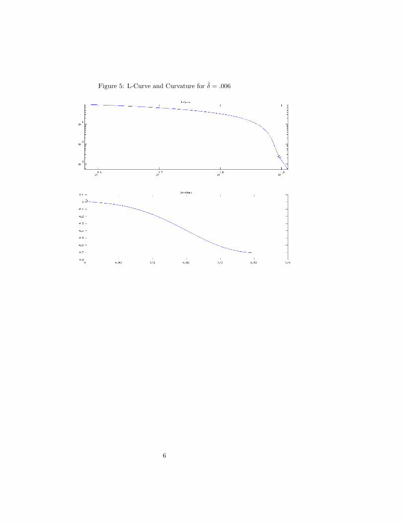
Figure 5: L-Curve and Curvature for δ̂ = .006

6

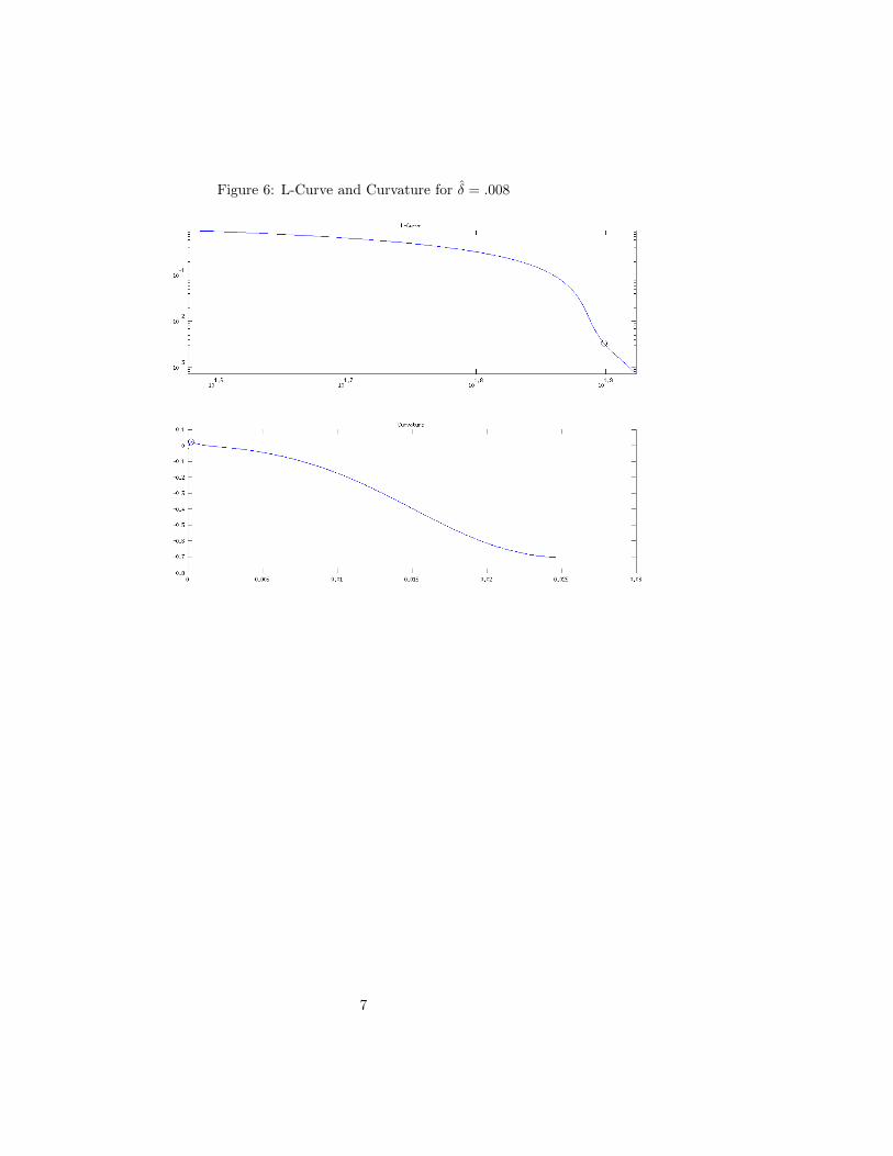
Figure 6: L-Curve and Curvature for δ̂ = .008

7

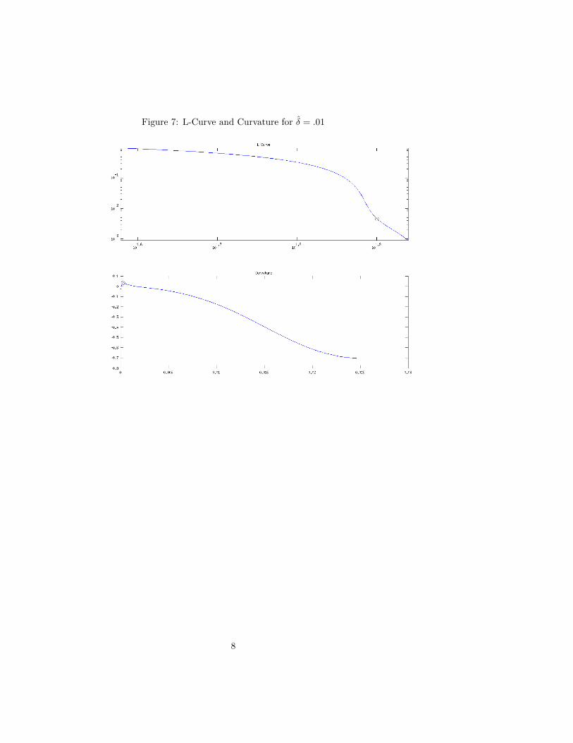
Figure 7: L-Curve and Curvature for δ̂ = .01

8

Figure 8: L-Curve and Curvature for δ̂ = .03

9

Figure 9: L-Curve and Curvature for δ̂ = .05

10

Figure 10: L-Curve and Curvature for δ̂ = .07

11

Figure 11: L-Curve and Curvature for δ̂ = .1

12

Our distinctive L-curve mentioned at the beginning of the section were no-ticeably absent. Furthermore, the L-curve method was noted to have producedthe A heuristic approach would be inadequate, however the use of an optimiza-tion algorithm allowed the identification of C(βL):

δ̂ βL L2 Error S(βL) R(βL)0 4.8148e-05 15.3988 79.1448 0.000114670.002 0.00012778 24.733 78.6185 0.000652150.004 0.00017826 31.0852 78.5561 0.00140050.006 0.00021254 35.6234 78.7618 0.00229550.008 0.00024404 39.8981 79.1294 0.00335060.01 0.00027325 43.9161 79.6198 0.00453340.03 0.00085718 114.7885 82.4843 0.0288310.05 0.0021447 194.086 80.1575 0.0798130.07 0.0027401 213.3111 80.9815 0.125660.1 0.003457 229.8098 82.1937 0.19809

Fourth Order ExampleThe L-curve method was applied to the fourth order problem in the same

manner as the second order problem, with sinusoidal noise weighted from 0 to.1.

The curvature for the fourth order problems were much more noticeable.

13

Figure 12: L-Curve and Curvature for δ̂ = 0

14

Figure 13: L-Curve and Curvature for δ̂ = .002

15

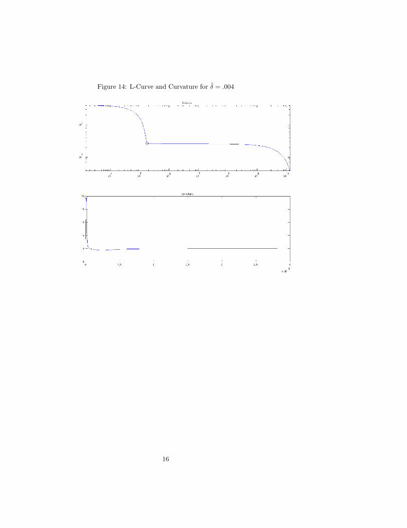
Figure 14: L-Curve and Curvature for δ̂ = .004

16

Figure 15: L-Curve and Curvature for δ̂ = .006

17

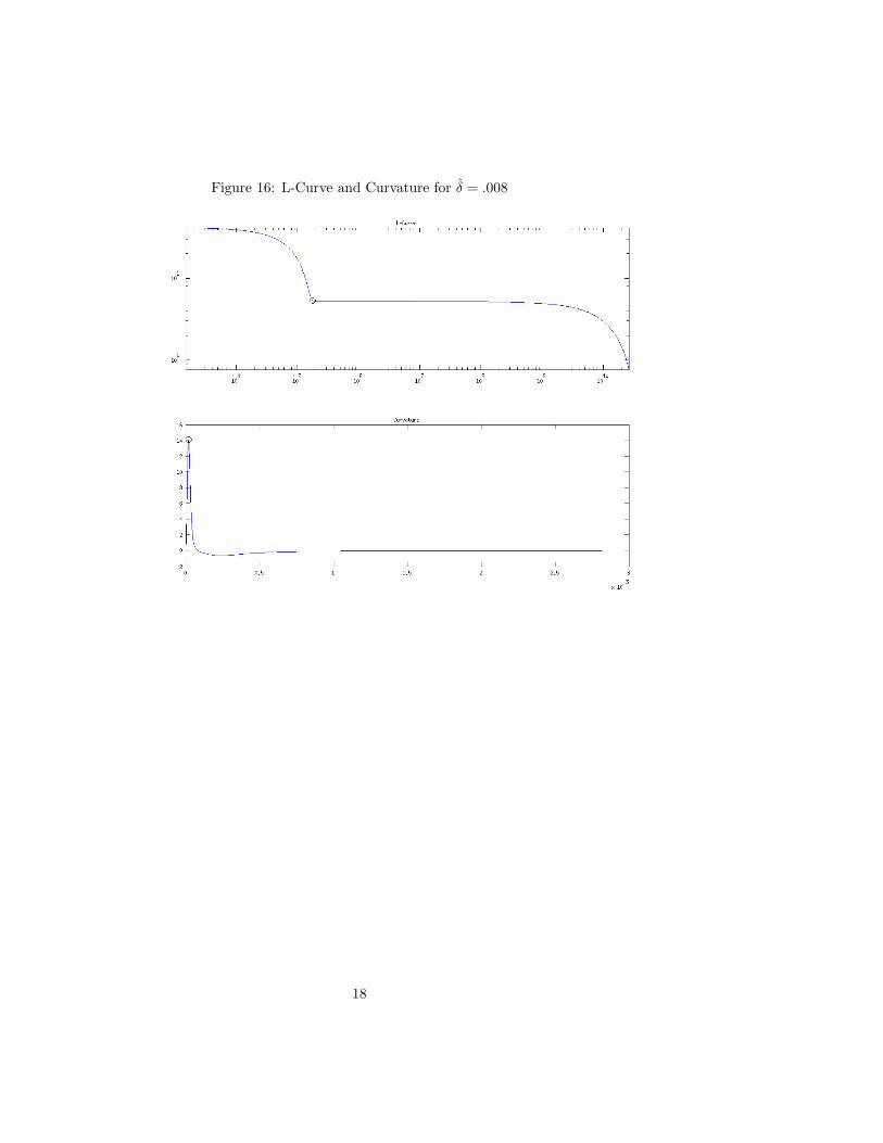
Figure 16: L-Curve and Curvature for δ̂ = .008

18

Figure 17: L-Curve and Curvature for δ̂ = .01

19

Figure 18: L-Curve and Curvature for δ̂ = .03

20

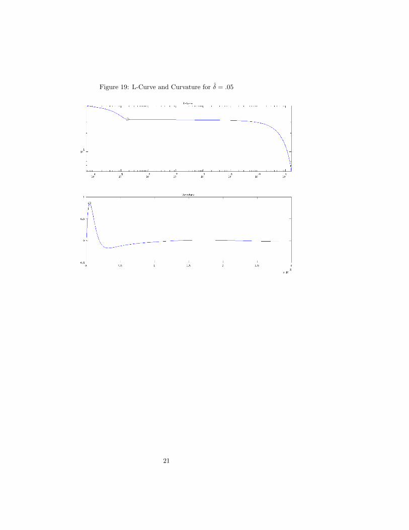
Figure 19: L-Curve and Curvature for δ̂ = .05

21

Figure 20: L-Curve and Curvature for δ̂ = .07

22

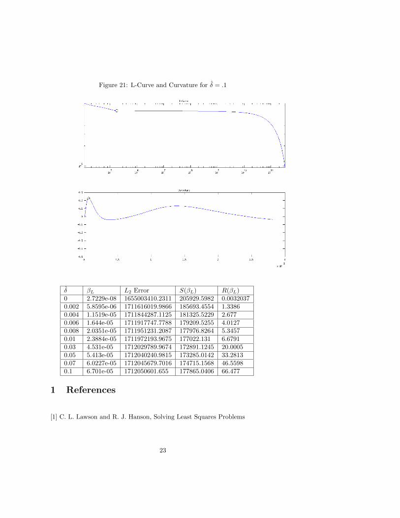
Figure 21: L-Curve and Curvature for δ̂ = .1

δ̂ βL L2 Error S(βL) R(βL)0 2.7229e-08 1655003410.2311 205929.5982 0.00320370.002 5.8595e-06 1711616019.9866 185693.4554 1.33860.004 1.1519e-05 1711844287.1125 181325.5229 2.6770.006 1.644e-05 1711917747.7788 179209.5255 4.01270.008 2.0351e-05 1711951231.2087 177976.8264 5.34570.01 2.3884e-05 1711972193.9675 177022.131 6.67910.03 4.531e-05 1712029789.9674 172891.1245 20.00050.05 5.413e-05 1712040240.9815 173285.0142 33.28130.07 6.0227e-05 1712045679.7016 174715.1568 46.55980.1 6.701e-05 1712050601.655 177865.0406 66.477

1 References

[1] C. L. Lawson and R. J. Hanson, Solving Least Squares Problems

23