LAUNCH VEHICLE PERFORMANCE ENHANCEMENT USING …

LAUNCH VEHICLE PERFORMANCE ENHANCEMENT USING

AERODYNAMIC ASSIST

Except where reference is made to the work of others, the work described in this thesis is my own or was done in collaboration with my advisory committee. This thesis does not

include proprietary or classified information.

_______________________Brian Robert McDavid

Certificate of Approval:

________________________ John E. BurkhalterProfessor EmeritusAerospace Engineering

_________________________ Roy J. Hartfield, Jr. ChairProfessorAerospace Engineering

________________________Brian ThurowAssistant ProfessorAerospace Engineering

_________________________George T. FlowersDeanGraduate School

LAUNCH VEHICLE PERFORMANCE ENHANCEMENT USING AERODYNAMIC

ASSIST

Brian Robert McDavid

A Thesis

Submitted to

the Graduate Faculty of

Auburn University

in Partial Fulfillment of the

Requirements for the

Degree of

Master of Science

Auburn, AlabamaAugust 9th, 2008

iii


ASSIST


Permission is granted to Auburn University to make copies of this thesis at its discretion, upon request of individuals or institutions and at their expense. The author reserves all

publication rights

Signature of Author

Date of Graduation

iv

VITA

Brian Robert McDavid was born on September 14th, 1982, in Brunswick, Maine

to Harry and Leslie McDavid. He graduated from Bob Jones High School in Madison,

Alabama and began attending Auburn University in 2001. As an undergraduate, he was

inducted into the Aerospace Engineering Honor Society Sigma Gamma Tau and the

national engineering honor society of Tau Beta Pi. Brian graduated Cum Laude in May

2006 with a Bachelor of Aerospace Engineering degree. He entered the Auburn

University Graduate School in Fall 2006 to pursue a Master of Science degree in

Aerospace Engineering. On December 29th, 2006, Brian married his beautiful wife Nicole

(Cann) McDavid.

v

THESIS ABSTRACT


ASSIST


Master of Science, August 9 2008(B.A.E., Auburn University, 2006)

66 Typed Pages

Directed by Roy J. Hartfield, Jr.

A complete preliminary design model of a three-stage solid-fuel launch vehicle

has been combined with a genetic algorithm to perform an optimization study with the

goal to enhance performance using aerodynamic assist. Three studies have been

completed which include improving the suborbital and orbital flights of a modern

intercontinental ballistic missile and improving on the orbital flight of a generic three-

stage launch vehicle. The performance is enhanced by varying the geometric definition of

the attached wing structure and the internal propellant geometry while the external

geometry remains constant. Initial system weights and propellant mass fractions were

found to decrease with the addition of the wing structure. Further enhancement involves a

payload increase by 10% with a negligible increase in system weight, and a propellant

mass decrease by 5.2% without impairing the flight performance.

vi

ACKNOWLEDGEMENTS

The author would like to thank Dr. Roy Hartfield and Dr. John Burkhalter for

their technical and professional guidance and support. The author also would like to

thank Dr. Murray Anderson, the author of the 3.1 IMPROVE Genetic Algorithm, without

which this thesis would not have been possible. The author would also like to thank his

parents Harry and Leslie and sister Amanda for their support and encouragement, and his

wife Nicole for all her patience and support provided throughout the graduate school

process.

vii

Style manual of journal used

The American Institute of Aeronautics and Astronautics Journal

Computer software used

Improve 3.1 Genetic Algorithm, Tecplot 10, Compaq Visual Fortran, Microsoft

Excel, Microsoft Word

viii

TABLE OF CONTENTS

LIST OF TABLES............................................................................................................. ix

LIST OF FIGURES ............................................................................................................ x

NOMENCLATURE ......................................................................................................... xii

1.0 INTRODUCTION .................................................................................................. 1

2.0 MODEL BACKGROUND ..................................................................................... 3

2.1 GENETIC ALGORITHM .................................................................................. 3

2.2 ADVANTAGES OF THE GENETIC ALGORITHM ....................................... 5

2.3 PRELIMINARY DESIGN MODEL .................................................................. 8

2.3.1 OBJECTIVE FUNCTION AND GA INITIALIZATION.......................... 9

2.3.2 DESIGN AND MISSION PARAMETERS ............................................. 11

2.3.3 PREDICTIVE MODEL............................................................................ 15

3.0 VALIDATION...................................................................................................... 23

4.0 AERODYNAMIC PERFORMANCE ENHANCEMENT................................... 27

4.1 MINUTEMAN-III SUBORBITAL ENHANCEMENT................................... 29

4.1.1 SUBORBITAL IMPROVEMENT ........................................................... 31

4.1.2 ORBITAL IMPROVEMENT................................................................... 39

4.2 THREE-STAGE ORBITAL ENHANCEMENT.............................................. 43

5.0 SUMMARY.......................................................................................................... 47

REFERENCES ................................................................................................................. 49

ix

LIST OF TABLES

Table 1: GA Design Variables for Minuteman-III ........................................................... 12

Table 2: Constant Mission Parameters ............................................................................. 13

Table 3: Propellant Design Variables ............................................................................... 13

Table 4: Wing and Tail Design Parameters ...................................................................... 14

Table 5: Minuteman-III Parameters.................................................................................. 14

Table 6: Mass Property Components................................................................................ 22

Table 7: Minuteman-III Validation................................................................................... 24

Table 8: PBAA/AP/Al Characteristics (English Units) .................................................... 26

Table 9: MM3 Suborbital Enhancement........................................................................... 38

Table 10: MM3 Suborbital Mass Fractions ...................................................................... 38

Table 11: MM3 Orbital Enhancement .............................................................................. 43

Table 12: MM3 Orbital Mass Fractions............................................................................ 43

Table 13: Generic Three-Stage Orbital Enhancement ...................................................... 46

Table 14: Generic Three-Stage Mass Fractions................................................................ 46

x

LIST OF FIGURES

Figure 1: Tournament Algorithm........................................................................................ 4

Figure 2: Crossover............................................................................................................. 7

Figure 3: Mutation .............................................................................................................. 8

Figure 4: Optimization Model Outline ............................................................................. 10

Figure 5: GA Population and Generation Setup ............................................................... 12

Figure 6: Bell Nozzle Schematic30.................................................................................... 18

Figure 7: Circular Arc Airfoil30 ........................................................................................ 20

Figure 8: Minuteman-III Validation Model...................................................................... 25

Figure 9: Air Density vs. Altitude..................................................................................... 27

Figure 10: Minuteman-III Dynamic Pressure ................................................................... 28

Figure 11: Minuteman-III ................................................................................................. 30

Figure 12: Minuteman-III with 2540 Payload .................................................................. 31

Figure 13: Altitude vs. Time (MM3-Wings) .................................................................... 33

Figure 14: Thrust vs. Time (MM3-Wings) ....................................................................... 33

Figure 15: Weight vs. Time (MM3-Wings)...................................................................... 34

Figure 16: GA Best Answer Convergence........................................................................ 34

Figure 17: Vehicle Diagram (MM3-Reduced Propellant) ................................................ 36

Figure 18: Convergence for MM3-Reduced Propellant ................................................... 36

Figure 19: Vehicle Diagram (MM3-Increased Payload) .................................................. 37

xi

Figure 20: Orbital MM3 GA Convergence....................................................................... 40

Figure 21: Orbital MM3 Wings ........................................................................................ 41

Figure 22: Orbital MM3 Altitude vs. Time ...................................................................... 41

Figure 23: Orbital MM3 Thrust Profile ............................................................................ 42

Figure 24: Orbital MM3 Convergence History ................................................................ 42

Figure 25: Generic Three-Stage Vehicle .......................................................................... 44

Figure 26: Three-Stage Altitude vs. Time ........................................................................ 45

Figure 27: Three-Stage Thrust Profile .............................................................................. 45

xii

NOMENCLATURE

m Mass Flow RateGA Genetic Algorithmr Propellant Burning Ratea Empirical Constantn Burning Rate IndexPc Chamber PressurePe Exit PressurePa Ambient PressureAb Burning Areaρb Solid Propellant Densityc* Characteristic VelocityR Specific Gas Constantγ Specific Heat RatioTc Chamber TemperatureA* Throat Areaue Exit VelocityT ThrustLf Fractional Nozzle LengthMW Molecular WeightMM3 Minuteman-IIIrpvar Propellant Outer Radiusrivar Propellant Inner Radiusfvar Fillet Radius Ratioeps Epsilon Star Widthptang Star Point Anglefn Fractional Nozzle Length Ratiodiath Throat Diameterrnose Nose Radius Ratiothet0 Initial Launch Angleb2tdb Tail Semi Spancrtdb Tail Root Chord Lengthtrt Taper Ratio TailtLEswp Sweep of Leading Edge in Tail FinsxTEtl Distance to Leading Edge of Tail Finsb2wdb Wing Semi Spancrwdb Wing Root Chord Lengthtrw Taper Ratio Wing

xiii

wLEswe Sweep of Leading Edge in WingsxLEw Distance to Leading Edge of Wings

1

1.0 INTRODUCTION

During the development of the Space Shuttle, the orbiter was designed with wings

which were anticipated for use only during reentry. The initial proposal for launch was

essentially a gravity turn launch which did not make use of lifting aerodynamics. During

the design process, launch studies were being conducted by Woltosz1,2 to ascertain the

most advantageous launch trajectory using a tool known as Rocket Ascent G-limited

Moment-balanced Optimization Program (RAGMOP). During this optimization exercise,

it was discovered that an “upside down” launch to orbit could increase payload by 20%

(about 8,000 lb at the time) 1,2. The reason for this improvement involved the more

efficient use of the orbiter wings for lift production in the upside down configuration

during the atmospheric portion of the ascent.

The payload advantage gained by the change in the ascent trajectory was entirely

free structurally for the Space Shuttle; however, based on the marked improvement in

performance associated with aerodynamic lifting for the shuttle, it is possible that

substantial improvement in net payload to orbit could be obtained for current launch

vehicles using aerodynamic lifting during the first stage burn despite the cost of adding

some mass in the form of wing structure (to the first stage). The potential payoff with

regard to achieving additional payload to orbit warrants the investigation described herein

which makes use of preliminary design level modeling and optimization tools. This study

includes physical modeling of the system components and digitally flying the launch

2

vehicle fitted with candidate wing design configurations through candidate ascent

trajectories. Using this general approach to preliminary design, researchers at Auburn

University have demonstrated substantial performance improvement for a Minotaur-type

vehicle using preliminary design level tools and a genetic algorithm3. The current

investigation uses the same preliminary design tools and includes wings to explore the

viability of the concept of using aerodynamic lifting during first phase ascent for a

generic vehicle. Two optimization studies have been completed for this thesis with the

goal of maximizing payload to orbit. The first study was conducted while changing only

the geometric definition of the add-on wing configuration (semi-span, root chord, tip

chord, sweep angle, taper ratio, and position). The first study includes a suborbital

optimization and an orbital optimization. The second study optimized an orbital launch

vehicle similar to the Minuteman-III from the “ground-up”.

The vehicle configuration for both studies uses a three-stage solid-fuel propulsion

system. The published fuel for the Minuteman-III is polybutadiene-acrylic acid with

ammonium perchlorate and aluminum (PBAA/AP/Al). PBAA has been hardwired in the

model as the propellant selection for every study in this thesis to ensure that performance

gains are associated with the geometric design and aerodynamics rather than with

propellant characteristics. Higher overall performance is expected from launch vehicles

which incorporate advanced design optimization methods, aerodynamic lifting and

advanced propellant chemistry. The propellant choice is fixed, but the grain geometry is

selected by the genetic algorithm.

3

2.0 MODEL BACKGROUND

2.1 GENETIC ALGORITHM

Genetic algorithms (GAs) are a powerful class of evolutionary computing tools in

which elements from biology such as reproduction, inheritance, mutation, selection, and

fitness, are used to solve very complex problems in a wide range of applications. John

Holland presented the method of applying the evolutionary process to solve scientific,

mathematical, and engineering problems in his 1975 book Adaptation in Natural and

Artificial Systems4. The benefits of using a GA to design and optimize a model in a set

design space have been well documented. A few specific aerospace applications include

the design and optimization of propellers5, freight truck aerodynamics6, wings and

airfoils7,8,9,10, rockets11,12, missiles13,14,15,16,17,18, flight trajectories19, spacecraft

controls20,21, and turbines22,23,24.

Genetic algorithms find an optimized solution by breeding new sets of data

(members) over a defined number of generations. The process starts by randomly creating

the first set of members based on a user specified design space. The user constricts the

minimum and maximum values for each design parameter. Each individual member is a

possible solution to the problem. Koza25, who worked with Holland to pioneer the first

batch of GAs, states that the genetic algorithm transforms a population (set) of

individuals (or members), each with an associated fitness value, into a new generation of

4

the population using reproduction, crossover, and mutation. Specifically, each member is

analyzed by the performance codes of the design model, and a fitness is assigned to each

member based on how well the member’s performance matched the objective function.

The final solution is the member that has the best fitness at the end of the last generation.

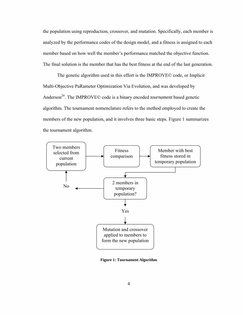
The genetic algorithm used in this effort is the IMPROVE© code, or Implicit

Multi-Objective PaRameter Optimization Via Evolution, and was developed by

Anderson26. The IMPROVE© code is a binary encoded tournament based genetic

algorithm. The tournament nomenclature refers to the method employed to create the

members of the new population, and it involves three basic steps. Figure 1 summarizes

the tournament algorithm.

Figure 1: Tournament Algorithm

Two members selected from

current population

Fitness comparison

Member with best fitness stored in

temporary population

2 members in temporary

population?

Mutation and crossover applied to members to

form the new population

No

Yes

5

First, two members of the current population are selected at random and their fitness

values are compared. The member having the better fitness moves to a temporary

population, and the other goes back to the current population. The process repeats to

generate a two member temporary population. Mutation and crossover operations are

performed on the two members in the temporary population, creating two new members

which are placed into the new population. This process continues until the new

population is filled with the correct number of members. The tournament method

therefore creates a new population with members having characteristics, or heredity, from

the previous population but in different combinations which may result in improved

fitness.

In addition to generating the members of the new population via tournament,

elitism is employed. Elitism takes the best performing member of the current population

and moves it to the next population without changing it at all. This is to safe-guard

against the mutated members all performing worse than the best member of the previous

population and sending the GA backwards. Elitism and tournament selection ensure that

the GA will find solutions that continually approach the target fitness. It should be noted

that the use of elitism, particularly with small populations can materially reduce the

genetic diversity of the population and care should be taken to address the adequacy of

the population size when using this option.

2.2 ADVANTAGES OF THE GENETIC ALGORITHM

There are several reasons why the genetic algorithm was chosen for this effort

instead of a gradient marching method. Gradient methods march toward a local

6

maximum or minimum by taking small steps that are proportional to the gradient of the

function. This requires that the objective function be differentiable in every independent

variable. If the function is not completely differentiable, then a singularity will develop

and the ability of the routine to march towards a maximum or minimum will be ruined. In

many systems it is impossible for the objective function to be completely differentiable.

For example, propellant type is not differentiable. A second problem with gradient

methods is that convergence to local optima is more common in design spaces with many

variables. The current preliminary design model requires 37 parameters, and their

derivatives are not easily ascertained. While the GA has a greater likelihood finding a

global optimum solution, obtaining this solution is not guaranteed. However, recent

techniques such as mutation and crossover help the GA to approach the global solution.

Mutation and crossover are powerful tools that help prevent genetic algorithms

from becoming stuck in a local optimum. A design variable is represented in the

IMPROVE© genetic algorithm by a binary string such as 101100101. When the

tournament selects two members to move to the next population, crossover is one of the

methods used to produce the new member, or offspring. The IMPROVE© code uses

single point crossover. In single point crossover, a location is chosen in the binary string

of each parent, and the remaining alleles are swapped from one parent to the other.

Crossover is more easily described by looking at a simple one offspring example as

shown in Figure 2. The numbers in bold are the values transferred to the offspring.

7

Figure 2: Crossover

When crossover is applied, the offspring takes one section of each parent’s genes. The

point at which the parent string is broken depends on the randomly selected crossover

point. Crossover occurrence is based on a set probability within the genetic algorithm

setup file, so sometimes the parent is directly copied to the offspring.

The second function that the genetic algorithm employs is mutation. After the

tournament selection and crossover, some of the offspring has been copied directly from

the parents, and the others have been affected by crossover. In order to ensure genetic

diversity, a small chance allowed for mutation is allowed. Each variable in the model is

represented by a binary string. The 1s and 0s that form a binary string are called alleles.

All of the members and their alleles are looped through, and if the allele is selected for

mutation, it is either changed by a small amount or replaced with a new value. Figure 3

shows an example of mutation. The allele in bold has been chosen for mutation and the

result is a change from a 0 to a 1.

Parent 11011010010100110

Parent 20011010110110101

Offspring0011010010100110

8

Figure 3: Mutation

If the GA approaches a local solution, this random change is very useful because it very

often creates a new member that is an improvement and can escape the trap of a local

solution.

2.3 PRELIMINARY DESIGN MODEL

As can be seen from References [5-24], the genetic algorithm is effective at

optimizing a problem when paired with a capable predictive model. The model in this

effort is a suite of FORTRAN codes used to model and simulate the flight of a three-stage

solid fueled rocket. The model was developed by Jenkins, Hartfield, and Burkhalter15,

and was modified to include orbital trajectories by Bayley3. These codes accurately

predict and simulate the performance of a three-stage solid fueled rocket by modeling the

aerodynamics, mass properties, and propulsion. The six-degree of freedom code manages

all the other codes while it simulates the flight of the missile and updates the performance

characteristics synchronized in time. This approach and this particular model was

validated by Bayley using the Minotaur as a baseline for comparison.

101101011001

101111011001

9

2.3.1 OBJECTIVE FUNCTION AND GA INITIALIZATION

The results of the flight are used to determine the fitness (or how well the member

met the desired optimization goals). The fitness is calculated by sending the appropriate

performance values into the objective function, with the output being the fitness. In this

model, the objective function is a quantitative measure that the GA uses to determine

which members have better performance. Two of the objective functions for this model

are to match a user specified orbital altitude and orbital velocity. These specified values

are chosen before the GA is started. After each member is digitally flown through the

model, values for the orbital altitude and velocity are obtained. Since two of the goals are

to match these values, the objective function compares the obtained value to the desired

value by using equations 1 and 2.

altorb

altorbaltanswer

11 (1)

vorb

vorbvanswer

12 (2)

If these were the only two desired goals, the fitness would be

21 answeranswerfitness (3)

In order to reach the desired altitude and velocity, answer 1 and answer 2 must be

minimized. As answer 1 approaches zero, the actual altitude becomes closer to the

desired altitude. Therefore, the member with the smallest value for the fitness is the best

performing member of the population and its characteristics are carried over into the next

generation. A second method of determining the fitness, pareto, could be used instead of

equation 3. Pareto style optimization separates the goals and attempts to minimize each

10

answer individually instead of the combined answer. Pareto was not used for the studies

in this thesis.

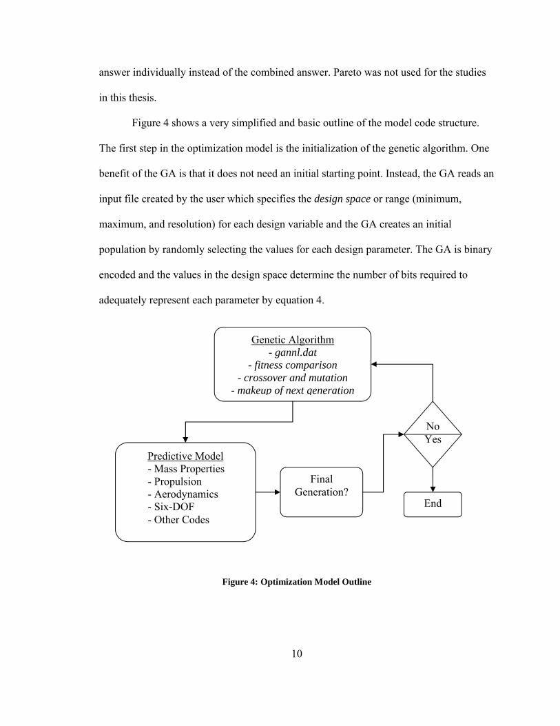
Figure 4 shows a very simplified and basic outline of the model code structure.

The first step in the optimization model is the initialization of the genetic algorithm. One

benefit of the GA is that it does not need an initial starting point. Instead, the GA reads an

input file created by the user which specifies the design space or range (minimum,

maximum, and resolution) for each design variable and the GA creates an initial

population by randomly selecting the values for each design parameter. The GA is binary

encoded and the values in the design space determine the number of bits required to

adequately represent each parameter by equation 4.

Figure 4: Optimization Model Outline

Genetic Algorithm- gannl.dat

- fitness comparison- crossover and mutation

- makeup of next generation

Predictive Model - Mass Properties - Propulsion - Aerodynamics - Six-DOF - Other Codes

Final Generation?

NoYes

End

11

12ln

minmaxln

resolutionnbits (4)

The variables in equation 4 are discussed in section 2.3.2. The number of bits required for

each parameter is important because the total number of bits influences the recommended

population size (n) by

nbitsn )0.3( (5)

A large population size is usually needed for a complicated design problem with a large

design space. The maximum population size that the IMPROVE© code can use is set at

400. The recommended number of generations is not as explicitly defined; however a

larger number of generations is more likely to produce an optimum solution. The trade-

off is that a large number of generations and a large population size can lead to

significant computer run times. It is up to the user to determine the appropriate number of

generations and to ascertain whether the solution produced is adequate.

2.3.2 DESIGN AND MISSION PARAMETERS

A section of the gannl.dat setup file used for this study is seen in Table 1. Figure

5 shows a section from the setup file that the GA reads to set the number of populations

and generations. Table 1 and Figure 5 show how the GA reads the design variables and

how the maximum, minimum, resolution, size of the population, and number of

generations are specified. The first column is a truncated description of the design

variable name, followed by the maximum, minimum, and resolution values. The

population size and number of generations are listed at the end.

12

Table 1: GA Design Variables for Minuteman-III

Parameter Maximum Minimum Resolutionrpvar1 0.8000 0.2000 0.0100 rivar1 0.9900 0.0100 0.0100 fvar1 0.2000 0.0100 0.0100 eps1 0.9700 0.1000 0.1000

ptang1 50.0000 10.0000 1.0000 fn1 0.9900 0.6000 0.0100

diath1 35.0000 5.0000 0.1000 rpvar2 0.8000 0.2000 0.0100 rivar2 0.9900 0.0100 0.0100 fvar2 0.2000 0.0100 0.0100 eps2 0.9700 0.5000 0.1000

ptang2 50.0000 10.0000 0.1000 fn2 0.9900 0.6000 0.0100

diath2 35.0000 5.0000 0.1000 rpvar3 0.8000 0.2000 0.0100 rivar3 0.9900 0.0100 0.0100 fvar3 0.2000 0.0100 0.0100 eps3 0.9700 0.5000 0.1000

ptang3 50.0000 10.0000 0.1000 fn3 0.9900 0.6000 0.0100

diath3 35.0000 5.0000 0.1000 rnose 0.7500 0.5000 0.0100 thet0 89.0000 70.0000 1.0000 b2tdb 1.4000 0.1000 0.1000 crtdb 1.2000 0.1000 0.1000

trt 0.9900 0.5000 0.0100 tLEswp 25.0000 5.0000 0.1000 xTEtl 0.9900 0.5000 0.1000 dele0 15.0000 0.0000 0.1000

timeb1 7.0000 0.1000 0.1000 timeb2 35.0000 7.0000 0.1000 timeee 90.0000 15.0000 1.0000 b2wdb 1.5000 0.1000 0.1000 crwdb 1.2000 0.1000 0.1000

trw 0.9900 0.5000 0.1000 wLEswe 25.0000 5.0000 0.1000

xLEw 0.6500 0.0500 0.1000

Figure 5: GA Population and Generation Setup

The launch location must be specified in order to accurately simulate an orbital

trajectory. Table 2 lists four mission parameters that are constant among all the different

optimization cases.

13

Table 2: Constant Mission Parameters

The desired system mass is another important mission parameter, however the

appropriate value is different based on which optimization case is being considered. For

example, the validation of the Minuteman-III has a desired system mass of 79,432 lbm,

whereas in cases where the wings are employed to reduce required propellant mass

through aerodynamic lifting the desired system mass is smaller. These are discussed in

more detail in the appropriate section of this thesis.

The optimization starts with the GA generating a set of 37 design parameters to

describe the launch vehicle. The geometric variables that describe the propellant for each

stage, as well as two external variables are shown in Table 3.

Table 3: Propellant Design Variables

Stages 1, 2, and 3 GA VariablePropellant Outer Radius Ratio rpvarPropellant Inner Radius Ratio rivar

Fillet Radius Ratio fvarEpsilon Star Width eps

Star Point Angle ptangFractional Nozzle Length Ratio fn

Throat Diameter diath

OtherNose Radius Ratio rnose

Initial Launch Angle thet0

Five variables are required to describe the wings/tails as seen in Table 4. All geometric

variables are non-dimensionalized by the body diameter.

Launch Site Vandenberg AFB, CA (34.6° N, 120.6° W)Launch Direction Due North (0° Azimuth or i = 90°/polar orbit)

Desired Orbital Velocity 22,000 ft/sDesired Orbital Altitude 750,000 ft

14

Table 4: Wing and Tail Design Parameters

Wings/Tails GA VariableSemispan b2wdb / b2tdb

Root Chord crwdb / crtdbTaper Ratio trw / trt

Leading Edge Sweep Angle wLEswe / tLEswpLeading Edge Location xLEw / tLEtl

The first study takes the Minuteman-III missile and attempts to increase the

payload/reduce the propellant weight, therefore certain external geometric parameters are

hardwired into the predictive model based on Minuteman-III data. These parameters are

shown in Table 5. The payload is the only parameter that changes in some of the

optimization cases. The second study does not constrain the vehicle to match the

Minuteman-III values, therefore the only value hardwired into the model is the stage

propellant.

Table 5: Minuteman-III Parameters

Parameter Minuteman-III ValuePayload* 2,540 lbm

Stage 1 Length 295.20 inStage 1 Diameter 66.00 inStage 1 Propellant PBAA/AP/Al



Constants such as material densities, program limits, target location, and physical

constants such as the radius of the earth are contained in a file called YYvar.dat.

These values can be changed easily if necessary to support new data.

15

2.3.3 PREDICTIVE MODEL

Propulsion

The propulsion code is the first to be called after the genetic algorithm is

initialized. This model analyzes the basic thrust performance and creates a full sea-level

thrust profile. Since the vehicle in this effort is three stages, the propulsion model is

called three times and the propulsion characteristics are determined for each stage

separately and in sequence. The basic theory in this model assumes steady-state

operation, which requires that the mass produced by the burning propellant is equal to the

mass output through the nozzle. Detailed derivations of the equations presented here can

be found in Sutton27. The burning rate is modeled by the empirical equation

ncapr (6)

where a is an empirical constant, n is the burning rate index, and Pc is the chamber

pressure. The mass flow rate of hot gas generated by the burning propellant and flowing

away from the motor is given by

bbrAm

(7)

where Ab is the burning area of the propellant grain, and ρb is the solid propellant density

prior to the motor start.

The burning area of the propellant can be tedious to calculate by hand, but

computers have made this process much simpler. Star grains and wagon wheel grains are

considered for this vehicle. The star and wagon wheel equations have been extensively

developed by Barrere34 and reviewed by Hartfield29. It is important to note that the

maximum burn area corresponds to the maximum chamber pressure, and for a star grain

16

the maximum burn area will always occur at the beginning of the burn or at the end of

phase II. Due to this fact, an initial check on chamber pressure is done once a design is

determined so that the thickness of the can be determined and a precise estimate of the

case weight can be calculated.

Isentropic flow is assumed through the nozzle, and the characteristic velocity is

defined as

12

1

2

1*

cRTc (8)

where Tc is the chamber temperature and gamma is defined by the propellant.

The relationships of isentropic flow can be used to express the mass flow rate through the

nozzle as

)1(2

1

1

2*

c

c

RT

Apm (9)

*

*

c

Apm c

(10)

where pc is the chamber pressure, A* is the throat area, R is the specific gas constant, Tc

is the chamber temperature, gamma is the specific heat ratio, and c* is the characteristic

velocity.

The chamber pressure can be expressed by

n

bt

bc ca

A

AP

1

1

* (11)

Assuming adiabatic, steady, 1-D flow, the exit velocity is

17

1

11

2

c

ece P

PRTu (12)

The thrust of the rocket motor is finally determined by

aeee PPAumT

(13)

A bell shaped nozzle is employed for this model because it is desirable to have a

nozzle that is minimum weight while not sacrificing performance. The geometric design

of the nozzle has been taken from Ref. 16 and Ref. 30. If a conical nozzle is used for

comparison, then the relative performance and relative weight can be determined. The

conical nozzle is a 15 degree half cone with a given expansion ratio and throat diameter.

The bell nozzle has the same expansion ratio and throat diameter, but the mass is

significantly lower. The length of the bell nozzle can be determined from equation 14,

where Lf is the fractional nozzle length and the denominator is the equivalent known

conical nozzle length.

cone

bellf L

LL

15

(14)

The bell nozzle diagram is shown in Figure 6.

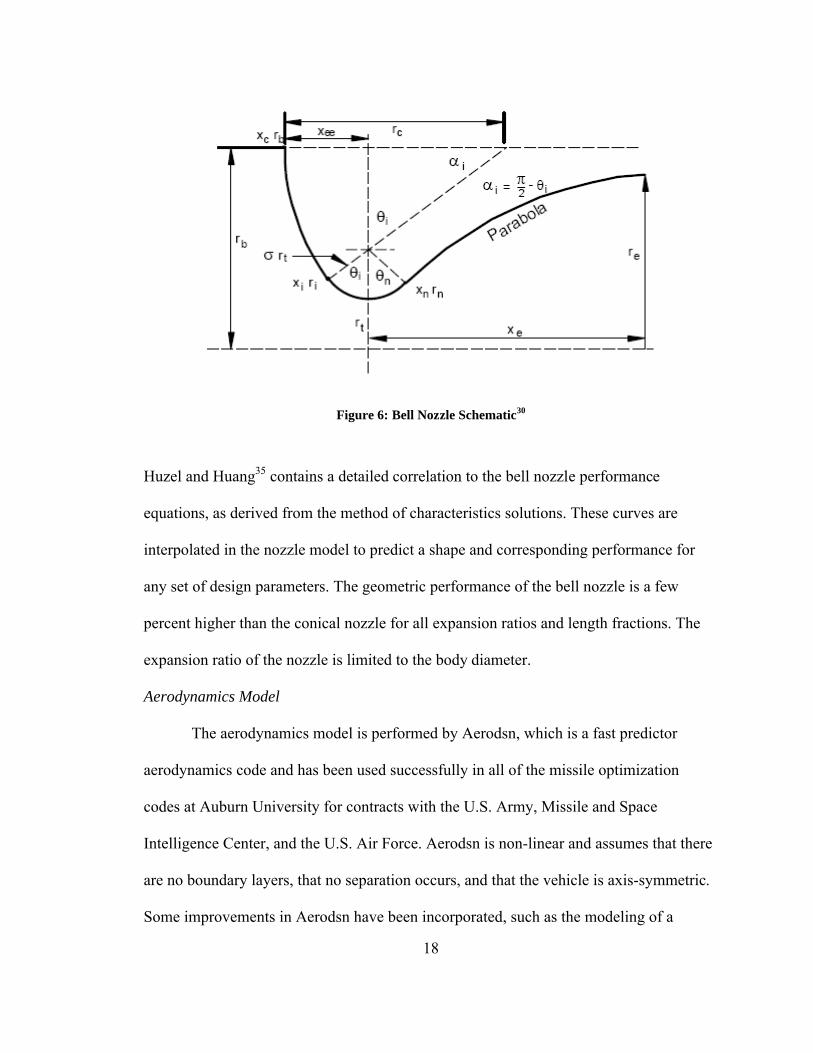
18

Figure 6: Bell Nozzle Schematic30

Huzel and Huang35 contains a detailed correlation to the bell nozzle performance

equations, as derived from the method of characteristics solutions. These curves are

interpolated in the nozzle model to predict a shape and corresponding performance for

any set of design parameters. The geometric performance of the bell nozzle is a few

percent higher than the conical nozzle for all expansion ratios and length fractions. The

expansion ratio of the nozzle is limited to the body diameter.

Aerodynamics Model

The aerodynamics model is performed by Aerodsn, which is a fast predictor

aerodynamics code and has been used successfully in all of the missile optimization

codes at Auburn University for contracts with the U.S. Army, Missile and Space

Intelligence Center, and the U.S. Air Force. Aerodsn is non-linear and assumes that there

are no boundary layers, that no separation occurs, and that the vehicle is axis-symmetric.

Some improvements in Aerodsn have been incorporated, such as the modeling of a

19

variable body diameter. More accurate computational fluid dynamic (CFD) simulations

are available; however the high computational cost makes CFD an unreasonable choice

for genetic algorithm applications where thousands of missiles are simulated under a

broad range of flight conditions.

Aerodsn generates aerodynamic databases based on the vehicle geometry and

other necessary parameters. Empirical curve fits of wind tunnel data are performed and

aerodynamic constants are determined over a wide range of flow conditions. The vehicle

geometry, initial constants, and empirical data are combined to generate an aerodynamic

database to describe the flight conditions. Aerodsn can model either a cone or an ogive

shape for the nosecone and assumes the body is cylindrical in shape; this study uses an

ogive nosecone. The vehicle is smooth except for the first stage which contains the wing

and tail set. The four canards and four tail fins are set in a “+” configuration on the first

stage. The wing and tail locations on the first stage are GA variables. Vehicles with

different wing configurations are not analyzed because Aerodsn only allows for the

cruciform configuration for the wings and tails. Aerodsn also limits the camber of the

wings. Aerodsn requires an axis-symmetric vehicle and using camber is not allowed in

Aerodsn. Future improvements will allow for different wing configurations and for

camber to be used.

The diameter of the 1st stage must be equal to or greater than the diameter of the

2nd or 3rd stages. For the Minuteman-III, the 2nd and 3rd stage diameters are equal. For the

first study, the stage diameters are set to the Minuteman-III value. The second study

allows the 3rd stage diameter to be smaller than the 2nd stage diameter for the generic

three-stage vehicle. The aerodynamics model is initially called before liftoff with all the

20

stages stacked together, and then it is called after stage 1 burnout, after stage 2 burnout,

and after stage 3 burnout. Essentially, the aerodynamic properties are calculated every

time the vehicle geometry changes.

The properties calculated by Aerodsn are used in conjunction with the mass

properties model to calculate all the aerodynamic forces acting on the vehicle. The

aerodynamics of the vehicle is relatively unimportant to this work. The benefit of the

lifting wings and the negative of the aerodynamic drag is only a concern during the first

stage burn. The explanation for this is explained in more detail at the start of section 4.0.

Mass Properties

The mass properties code is another important piece of the model. The airfoil

section for both the wing and tail fin sets are assumed to be circular arc airfoils. It is

assumed that the wing has no camber and that the leading and trailing edges are identical.

A generic circular arc cross-section is shown in Figure 7.

Figure 7: Circular Arc Airfoil30

21

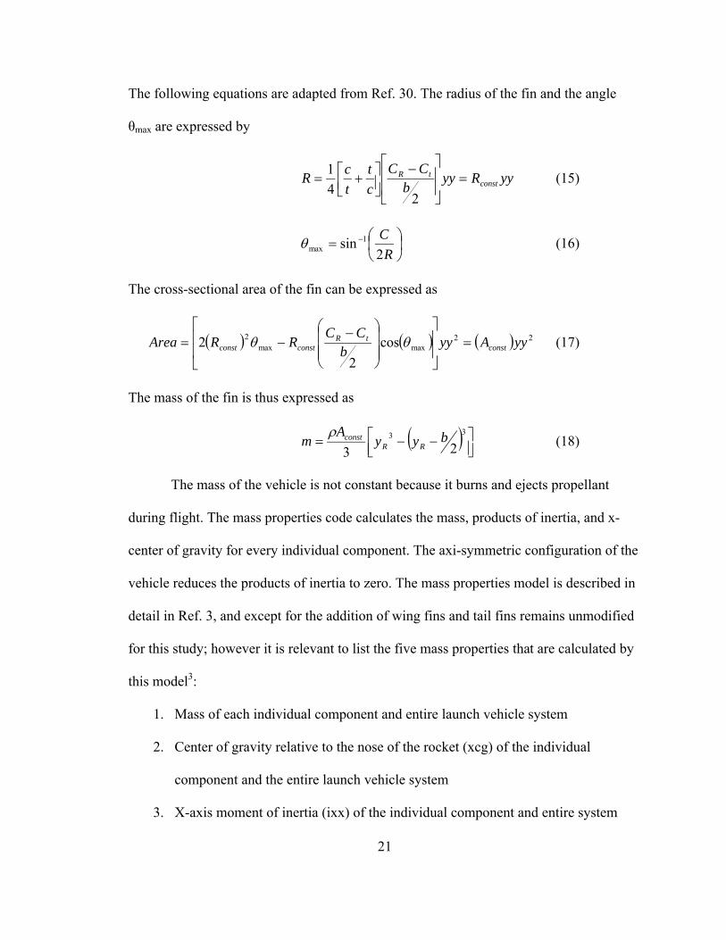
The following equations are adapted from Ref. 30. The radius of the fin and the angle

θmax are expressed by

yyRyyb

CC

c

t

t

cR const

tR

24

1(15)

R

C

2sin 1

max (16)

The cross-sectional area of the fin can be expressed as

22maxmax

2 cos

2

2 yyAyyb

CCRRArea const

tRconstconst

(17)

The mass of the fin is thus expressed as

33

23byy

Am RR

const(18)

The mass of the vehicle is not constant because it burns and ejects propellant

during flight. The mass properties code calculates the mass, products of inertia, and x-

center of gravity for every individual component. The axi-symmetric configuration of the

vehicle reduces the products of inertia to zero. The mass properties model is described in

detail in Ref. 3, and except for the addition of wing fins and tail fins remains unmodified

for this study; however it is relevant to list the five mass properties that are calculated by

this model3:

1. Mass of each individual component and entire launch vehicle system

2. Center of gravity relative to the nose of the rocket (xcg) of the individual

component and the entire launch vehicle system

3. X-axis moment of inertia (ixx) of the individual component and entire system

22

4. Y-axis moment of inertia (iyy) of the individual component and entire system

5. Z-axis moment of inertia (izz) of the individual component and entire system

The components that are analyzed by the mass properties code for the three-stage launch

vehicle are shown in Table 6.

Table 6: Mass Property Components

System Components Stages 1-2-3 Stage 1Blunt Nose Bulkhead Wings

Ogive Ignitor TailsPayload Motor Case

Electronics LinerInsulation

NozzlePropellant Grain

Dynamics Simulation

The six degree of freedom model (six-DOF) is the core analysis tool used to

determine performance. All the performance characteristics are calculated inside the six-

DOF. The six-DOF code can be considered the ‘project manager’ of the predictive

model. The digital flight of the model is initiated and completed using a 7-8th order

Runge-Kutta integration routine (RK78). The RK78 routine integrates the equations of

motion. The propulsion, mass properties, and aerodynamics models are all called from

the six-DOF to update parameters real-time during the flight. The integration process

continues until the vehicle reaches the apogee of the ballistic flight trajectory. The apogee

ideally corresponds to the orbital insertion point for a low-Earth, circular orbit. Once the

six-DOF is complete, the desired goals such as orbital altitude and orbital velocity are

sent to the genetic algorithm for analysis. The goal of the optimization is to minimize the

values obtained from the six-DOF with the desired values that are set prior to the

analysis.

23

3.0 VALIDATION

To be useful as design tools, computer models of physical systems require proof

of the validity of the physical model. Validation is the process of determining if the

physical system being modeled is correct. A validated model provides a degree of

confidence in the accuracy of the physical system and the results from an optimization

study which uses the model.

Individual components of the predictive model used in the current study have

been validated independently in previous studies. The solid propellant propulsion model

was developed and validated by Burkhalter28, Hartfield30, and Sforzini31. The

aerodynamics model, Aerodsn, has been an industry tool since 1990. Aerodsn and the

six-DOF flight dynamics simulator have been used and validated extensively by Hartfield

et al15,16,17.

The three-stage solid-fuel orbital flight model for this thesis was validated using

real world data for the Minuteman-III ICBM32,33. The Minuteman-III is a strategic

weapon system using a ballistic missile of intercontinental range. Although the

Minuteman-III was not designed to take a payload into orbit, it was chosen for this study

because it has a known configuration that reaches suborbital altitude and velocity. Using

the known data for the Minuteman-III, the GA is used to determine the unknown

parameters. An optimization is performed to develop a vehicle having similar

characteristics to the real-world example. If the model can produce a vehicle with very

24

similar parameters to the real vehicle, then the validity and uncertainty of the model can

be ascertained.

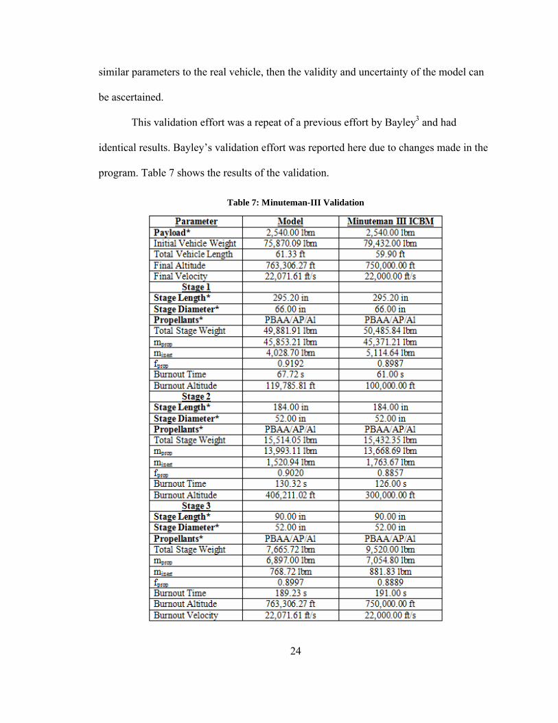
This validation effort was a repeat of a previous effort by Bayley3 and had

identical results. Bayley’s validation effort was reported here due to changes made in the

program. Table 7 shows the results of the validation.

Table 7: Minuteman-III Validation

25

Values in Table 7 listed in bold* were direct inputs based on known Minuteman-III data.

The rest of the parameters were determined by the GA. The results of the GA

optimization are very close to the published Minuteman-III data. An important validation

check is in the ability of the model to reproduce the performance characteristics such as

the final altitude (763,306.27 ft to 750,000.00 ft) and burnout velocity (22,071.61 ft/s to

22,000.00 ft/s). Stage weights burnout times match fairly closely as well. This validation

was performed with no wings and tails. Coincidently, an optimization case performed for

this study (discussed in section 4) that includes wings and tails was able to narrow down

on the altitude and velocity values by a large margin while only changing the system

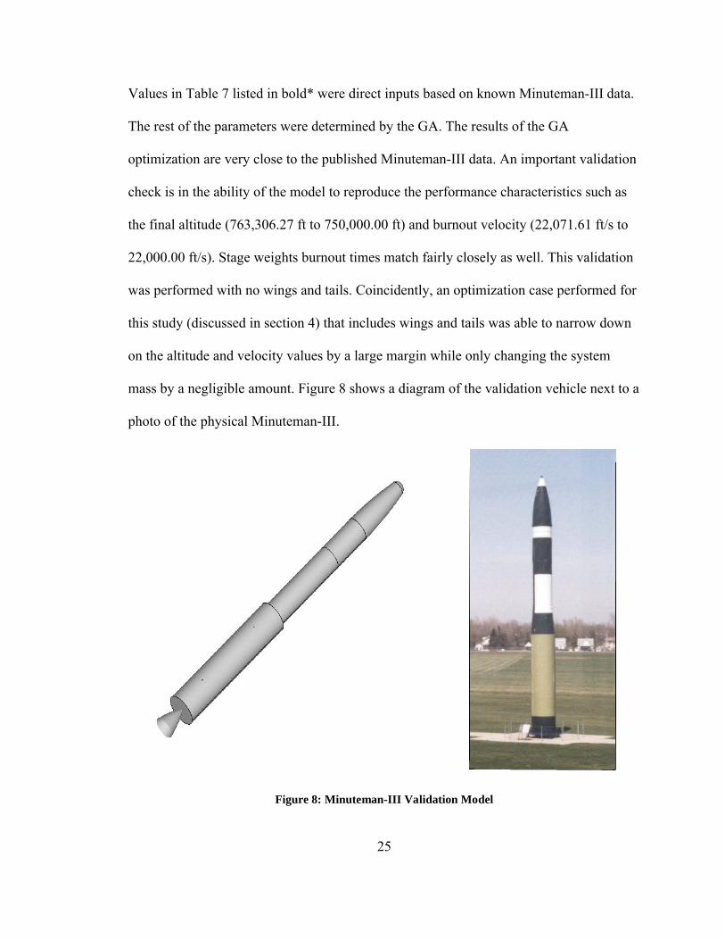
mass by a negligible amount. Figure 8 shows a diagram of the validation vehicle next to a

photo of the physical Minuteman-III.

Figure 8: Minuteman-III Validation Model

26

The fuel for each stage is PBAA/AP/Al. Table 8 shows a list of the characteristics of the

propellant.

Table 8: PBAA/AP/Al Characteristics (English Units)

Parameter Valuea 0.0285n 0.35

rho 0.064Tc 6159.67

gamma 1.24cstar 5700Tio 519MW 24.7

An important parameter to compare vehicles is the propellant mass fraction calculated by

inertfuel

fuelprop mm

mf

(19)

The vehicles with wings should have a smaller propellant mass fraction than the vehicles

without wings.

27

4.0 AERODYNAMIC PERFORMANCE ENHANCEMENT

As discussed in section 1.0, it is very likely that substantial improvement in net

payload to orbit could be obtained for current launch vehicles using aerodynamic lifting

during the first stage burn despite the cost of adding some mass in the form of wing

structure (to the first stage). Attaching the wing structure to the first stage makes the most

use of any possible aerodynamic lifting effects. As the vehicle climbs in altitude, the

density of the air molecules drastically decreases. The flight envelope where aerodynamic

forces are non-trivial is limited to the first-stage portion of the trajectory due to the

decrease in density. Figure 9 shows graphically how density decreases as altitude

increases. At 100,000 feet, the density is 1% of the sea-level value.

0

0.0005

0.001

0.0015

0.002

0.0025

0 20000 40000 60000 80000 100000 120000

Altitude (ft)

De

ns

ity

(s

lug

/ft^

3)

Figure 9: Air Density vs. Altitude

28

Another important parameter for spacecraft is the dynamic pressure because it can show

the point of maximum aerodynamic load on the vehicle. Dynamic pressure is described

by equation 19. Figure 10 shows the dynamic pressure for the first stage flight of the

Minuteman-III.

2

2

1VQ (19)

0

500

1000

1500

2000

2500

3000

0 20000 40000 60000 80000 100000 120000 140000Altitude (ft)

Dyn

amic

Pre

ssu

re (

lbf)

Figure 10: Minuteman-III Dynamic Pressure

The performance enhancement revolves around the wing and tail configuration. A

rocket with no fins is unstable, so fins are attached in order to aerodynamically stabilize

the vehicle at a specific trim angle. One of the purposes for the optimization studies

presented herein is to use the genetic algorithm to find a fin configuration that enables the

rocket to trim at a higher angle of attack. At the higher trim angle, the body and fin

system will have a higher normal force than the body alone. The trim angles for the

vehicles in this study range from slightly above 0 degrees to a maximum of 4.3 degrees.

29

Performance enhancement testing is divided into three groups with all tests

employing the wing and tail system. The propellant type is a constant and therefore is the

same for every optimization study. First, the Minuteman-III external body geometry is

kept constant to the validation model except for the addition of a wing and tail system.

Three optimization tests are performed on this configuration with a desired suborbital

altitude of 750,000 feet and velocity of 22,000 ft/s:

1. The payload and propellant fuel mass are held constant.

2. The payload is increased by 10% for a system with wings and for the

validation system.

3. For both payloads, the desired propellant fuel mass and the desired initial

system weight are reduced.

Second, the three-stage Minuteman-III geometry is used to attempt to achieve

low-earth orbit conditions of 2,430,000 feet and 24,550 ft/s with a payload of 1,000

pounds. Tests are conducted with the validation Minuteman-III system (no wings) and

compared to an enhanced Minuteman-III configuration equipped with the wing and tail

system.

The third group of tests compares the result of a generic three-stage launch

vehicle optimization performed by Bayley3 to the result of the same optimization

procedure using the wing and tail system.

4.1 MINUTEMAN-III SUBORBITAL ENHANCEMENT

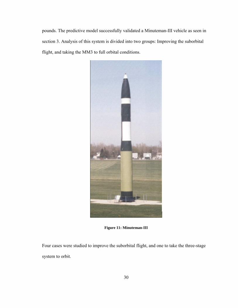
The Minuteman-III (Figure 11) is a three-stage solid ICBM and achieves a

suborbital apogee of 750,000 feet and a speed of 22,000 ft/s. The payload is 2,540

30

pounds. The predictive model successfully validated a Minuteman-III vehicle as seen in

section 3. Analysis of this system is divided into two groups: Improving the suborbital

flight, and taking the MM3 to full orbital conditions.

Figure 11: Minuteman-III

Four cases were studied to improve the suborbital flight, and one to take the three-stage

system to orbit.

31

4.1.1 SUBORBITAL IMPROVEMENT

The first suborbital test was to improve on the performance (matching the desired

altitude and velocity) of the validation case by keeping the external geometry, propellant

type, and payload the same, but adding wings and tails to the first stage. The design

variables are the geometric definition of the wing and tail (Table 4) and the internal

geometry of the propellant. The optimized vehicle is shown in Figure 12.

Figure 12: Minuteman-III with 2540 Payload

The wings presented for this vehicle are unrealistic, but serve as a proof of

concept for the idea of enhancing performance through aerodynamic assistance. With a

more accurate structural analysis, the wings presented here would break off under the

load. An improvement to the model for future analysis should include more restrictions

32

on the semi-span and chord length to limit the aspect ratio. All the suborbital

enhancement cases have this issue. In addition, the model does not show fairings over the

variable diameter stage connections. The model contains a correction factor for the drag

computations.

The new vehicle weighed less and matched the desired values for altitude and

velocity much more closely than the original validation. This vehicle attained an altitude

of 750,007 ft, a speed of 22,000.8 ft/s, and total system mass of 74,935 lbm. Noticing that

this vehicle flies to 750,007 ft and the validation model flies to 763,306 ft, it is possible

that the mass savings could be due in part to the vehicle flying to a lower altitude.

However, the remaining test cases also closely match the desired altitude, and the initial

mass is shown to be further reduced when compared to the previous case.

The additional control provided by the wing and tail system allowed the trajectory

to more closely match the desired suborbital values than the original validation case. The

ballistic trajectory can be seen in Figure 13, the thrust profile in Figure 14, and the

velocity profile in Figure 15.

33

Figure 13: Altitude vs. Time (MM3-Wings)

Figure 14: Thrust vs. Time (MM3-Wings)

34

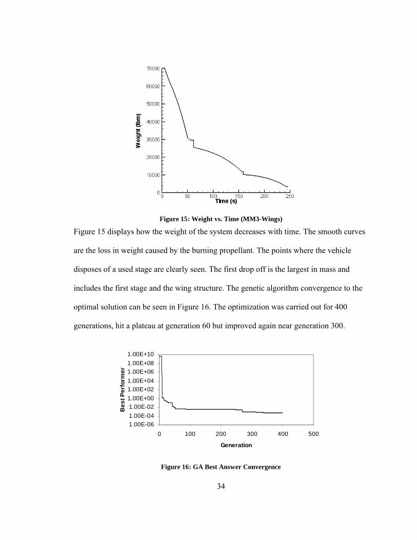
Figure 15: Weight vs. Time (MM3-Wings)

Figure 15 displays how the weight of the system decreases with time. The smooth curves

are the loss in weight caused by the burning propellant. The points where the vehicle

disposes of a used stage are clearly seen. The first drop off is the largest in mass and

includes the first stage and the wing structure. The genetic algorithm convergence to the

optimal solution can be seen in Figure 16. The optimization was carried out for 400

generations, hit a plateau at generation 60 but improved again near generation 300.

1.00E-06

1.00E-04

1.00E-02

1.00E+00

1.00E+02

1.00E+04

1.00E+06

1.00E+08

1.00E+10

0 100 200 300 400 500

Generation

Be

st

Pe

rfo

rme

r

Figure 16: GA Best Answer Convergence

35

The next suborbital test case kept the payload (2,540 lbm) and external geometry

constant but reduced the desired first stage fuel mass by 5.2% from 45,371 pounds to

43,000 pounds. A reduction in propellant translates into a direct reduction in costs.

Again, the only variables are the wing and tail definitions and the internal propellant

geometry. Figure 17 shows a diagram of the optimized vehicle. This vehicle has a 74

degree launch angle and attains an altitude of 749,992.6 feet, a velocity of 22,000.0 ft/s,

and weighs 72,402 pounds. This vehicle weighs 2,533 pounds less than the previous case.

From the previous design, the wings have progressed towards a more aerodynamic

efficient shape. The new, thinner shape of the wings has a lower induced drag. As will be

seen in subsequent diagrams, the general trend of evolution using the genetic algorithm is

that thinner wings are designed for the vehicles having the lowest initial system mass.

The previously mentioned issues concerning the unrealistic wings apply to this case.

These wings would break if the structural model was more accurate. Genetic algorithm

best performer convergence is shown in Figure 18.

36

Figure 17: Vehicle Diagram (MM3-Reduced Propellant)

1.00E-04

1.00E-02

1.00E+00

1.00E+02

1.00E+04

1.00E+06

1.00E+08

1.00E+10

0 100 200 300 400 500

Generation

Bes

t Per

form

er

Figure 18: Convergence for MM3-Reduced Propellant

The next test to improve the suborbital performance of the Minuteman-III was to

increase the payload by 10%, from 2540 pounds to 2794 pounds, with a negligible

increase in the initial system mass. The design variables are the wing and tail definitions

and the internal propellant geometry. The optimization produced a vehicle that matched

the desired goals closely and had an initial system mass of only a fraction more. The

37

vehicle is seen in Figure 19 and weighs 74,959 pounds, is launched at 71 degrees, reaches

an altitude of 749,997.5 feet, and reaches a speed of 22,000.2 ft/s. The structural issues

for the wings apply to this case. Future investigations will limit the aspect ratio further to

prevent this problem.

Figure 19: Vehicle Diagram (MM3-Increased Payload)

The convergence of the best performer is similar to the previous test cases, reaching an

optimum solution around the 60th generation and improving only slightly afterwards.

As a comparison to the previous case, the analysis that produced the Minuteman-

III validation model (no wings) was performed using the increased payload of 2,794

pounds. This optimization case produced a vehicle that reaches an altitude of 749,998

feet, a speed of 22,000.1 ft/s, and weighs 77648.2 pounds. The original MM3 validation

38

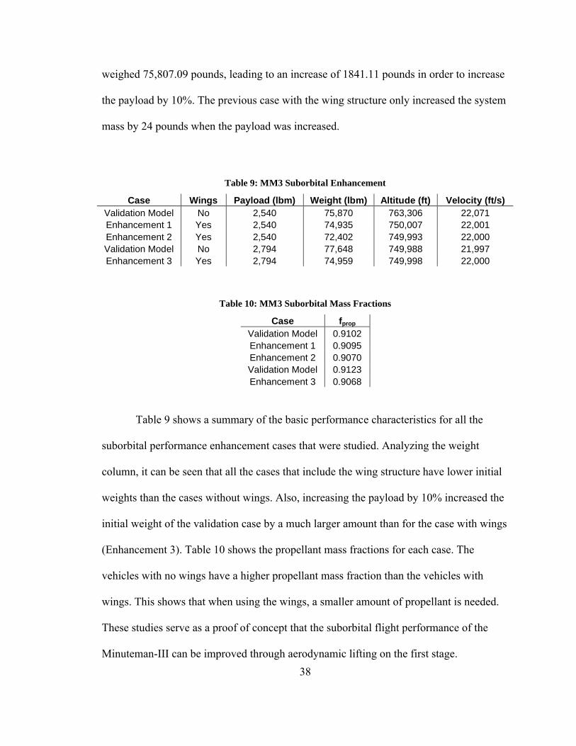
weighed 75,807.09 pounds, leading to an increase of 1841.11 pounds in order to increase

the payload by 10%. The previous case with the wing structure only increased the system

mass by 24 pounds when the payload was increased.

Table 9: MM3 Suborbital Enhancement

Case Wings Payload (lbm) Weight (lbm) Altitude (ft) Velocity (ft/s)Validation Model No 2,540 75,870 763,306 22,071Enhancement 1 Yes 2,540 74,935 750,007 22,001Enhancement 2 Yes 2,540 72,402 749,993 22,000Validation Model No 2,794 77,648 749,988 21,997Enhancement 3 Yes 2,794 74,959 749,998 22,000

Table 10: MM3 Suborbital Mass Fractions

Case fprop

Validation Model 0.9102Enhancement 1 0.9095Enhancement 2 0.9070Validation Model 0.9123Enhancement 3 0.9068

Table 9 shows a summary of the basic performance characteristics for all the

suborbital performance enhancement cases that were studied. Analyzing the weight

column, it can be seen that all the cases that include the wing structure have lower initial

weights than the cases without wings. Also, increasing the payload by 10% increased the

initial weight of the validation case by a much larger amount than for the case with wings

(Enhancement 3). Table 10 shows the propellant mass fractions for each case. The

vehicles with no wings have a higher propellant mass fraction than the vehicles with

wings. This shows that when using the wings, a smaller amount of propellant is needed.

These studies serve as a proof of concept that the suborbital flight performance of the

Minuteman-III can be improved through aerodynamic lifting on the first stage.

39

4.1.2 ORBITAL IMPROVEMENT

The Minuteman-III is not an orbital vehicle, but tests were conducted to

determine if the Minuteman-III geometry from the validated model could sustain a flight

to orbital conditions. After a successful design to orbit, a second test was performed with

the goal of enhancing performance through aerodynamic lifting during the first stage

burn. This section discusses these tests and compares the results.

The first test was to take the validation model to orbit. The desired goals were

changed from suborbital conditions to a desired altitude of 2,430,000 feet and desired

velocity of 24,550 ft/s. The payload was changed from the Minuteman-III suborbital

value of 2,540 pounds to a more typical orbital payload of 1,000 pounds. As before, the

only variables that are allowed to change are the wing and tail geometry definitions and

the internal propellant geometry. The genetic algorithm was able to converge to a design

that achieved the desired orbital conditions, reaching an altitude of 2,430,024 feet and a

velocity of 24,551 ft/s. The diagram of the vehicle is the same as previous Minuteman-III

validation configurations (such as Figure 8) because the external geometry is constant.

The vehicle weighs 75,760 pounds, which is similar to the 75,870 pounds that the

validation case weighs to reach suborbital conditions. This vehicle is 110 pounds lighter

than the validation case yet achieves a higher altitude and faster velocity. The 1,540

pound reduction in payload was directly applied to the first and second stage propellant

mass. The validation case had a first and second stage propellant mass of 45,371 pounds

and 13,668 pounds respectively, and the current vehicle has first and second stage

propellant mass of 46,750 pounds and 14,413 pounds respectively. Figure 20 shows the

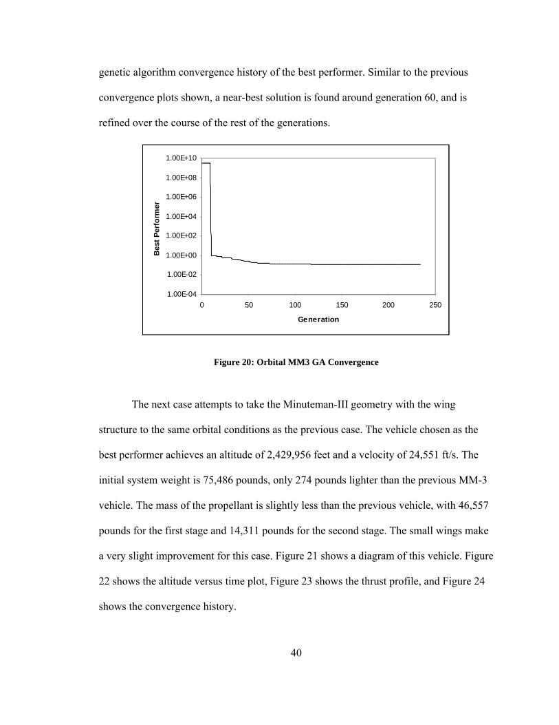
40

genetic algorithm convergence history of the best performer. Similar to the previous

convergence plots shown, a near-best solution is found around generation 60, and is

refined over the course of the rest of the generations.

1.00E-04

1.00E-02

1.00E+00

1.00E+02

1.00E+04

1.00E+06

1.00E+08

1.00E+10

0 50 100 150 200 250

Generation

Bes

t P

erfo

rmer

Figure 20: Orbital MM3 GA Convergence

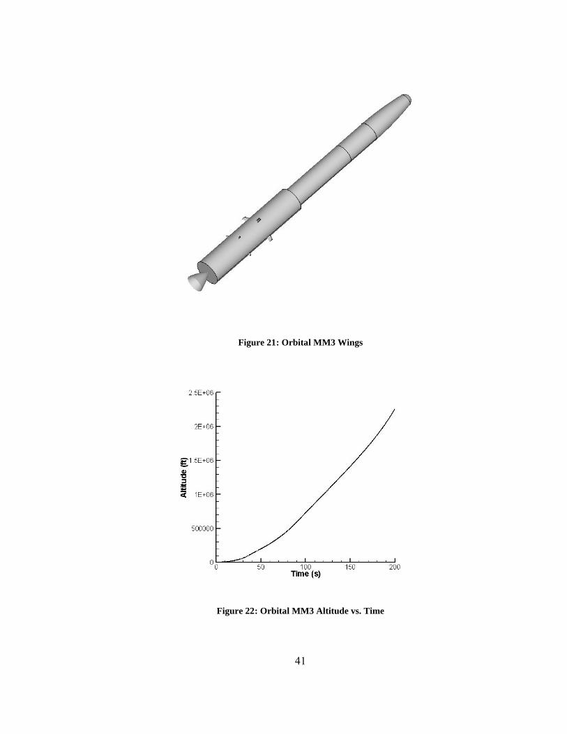
The next case attempts to take the Minuteman-III geometry with the wing

structure to the same orbital conditions as the previous case. The vehicle chosen as the

best performer achieves an altitude of 2,429,956 feet and a velocity of 24,551 ft/s. The

initial system weight is 75,486 pounds, only 274 pounds lighter than the previous MM-3

vehicle. The mass of the propellant is slightly less than the previous vehicle, with 46,557

pounds for the first stage and 14,311 pounds for the second stage. The small wings make

a very slight improvement for this case. Figure 21 shows a diagram of this vehicle. Figure

22 shows the altitude versus time plot, Figure 23 shows the thrust profile, and Figure 24

shows the convergence history.

41

Figure 21: Orbital MM3 Wings

Figure 22: Orbital MM3 Altitude vs. Time

42

Figure 23: Orbital MM3 Thrust Profile

1.00E-03

1.00E-01

1.00E+01

1.00E+03

1.00E+05

1.00E+07

1.00E+09

1.00E+11

0 100 200 300 400Generation

Be

st

Pe

rfo

rme

r

Figure 24: Orbital MM3 Convergence History

Table 11 summarizes the performance goals of the two orbital designs.

Table 12 shows the propellant mass fractions for these two vehicles. The propellant mass

43

fractions are very similar, and the fraction for the vehicle with wings is only slightly

smaller than for the vehicle without wings.

Table 11: MM3 Orbital Enhancement

Case Wings Payload (lbm) Weight (lbm) Altitude (ft) Velocity (ft/s)Validation Model No 1,000 75,760 2,430,024 24,551Enhancement 1 Yes 1,000 75,486 2,429,956 24,551

Table 12: MM3 Orbital Mass Fractions

Case fprop

Validation Model 0.91313Enhancement 1 0.91302

4.2 THREE-STAGE ORBITAL ENHANCEMENT

The generic three-stage solid fuel model includes more variables than the

validation model. The stage lengths and stage diameters are not hard-wired to match the

Minuteman-III and are included in the design space for the GA. Wall thickness

parameters were known for the MM3 but are calculated for the generic model, therefore

the initial system weight is on a different scale than for the MM3 cases. Due to this

discrepancy, the comparisons for vehicles with the wing structure to a baseline case are

done using the optimizations performed by Bayley3. The same design optimizations are

performed but with the addition of the wing structure and the results are compared.

The baseline vehicle attains an altitude of 2,439,276 feet, a velocity of 24,595 ft/s,

and has an initial system mass of 89,906 pounds. The specific details of the flight can be

seen in Ref. 3. The wing structure was added to this model and the optimization

performed again. The same wing and tail variables that were added to the Minuteman-III,

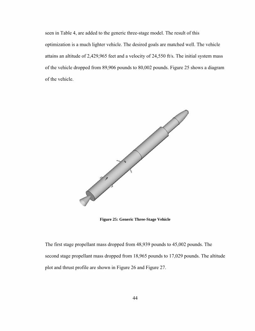
44

seen in Table 4, are added to the generic three-stage model. The result of this

optimization is a much lighter vehicle. The desired goals are matched well. The vehicle

attains an altitude of 2,429,965 feet and a velocity of 24,550 ft/s. The initial system mass

of the vehicle dropped from 89,906 pounds to 80,002 pounds. Figure 25 shows a diagram

of the vehicle.

Figure 25: Generic Three-Stage Vehicle

The first stage propellant mass dropped from 48,939 pounds to 45,002 pounds. The

second stage propellant mass dropped from 18,965 pounds to 17,029 pounds. The altitude

plot and thrust profile are shown in Figure 26 and Figure 27.

45

Figure 26: Three-Stage Altitude vs. Time

Figure 27: Three-Stage Thrust Profile

46

Table 13 shows a summary of the performance goals for the generic three-stage vehicles.

Table 13: Generic Three-Stage Orbital Enhancement

Case Wings Payload (lbm) Weight (lbm) Altitude (ft) Velocity (ft/s)3-Stage No 1,000 89,906 2,439,276 24,595

3-Stage Enhance Yes 1,000 80,002 2,429,965 24,550

Table 14: Generic Three-Stage Mass Fractions

Case fprop

3-Stage 0.90783-Stage Enhance 0.8904

Table 14 shows the propellant mass fractions for the generic three stage optimizations.

The vehicle with the wings has a slightly lower propellant mass fraction than the vehicle

without wings.

47

5.0 SUMMARY

Launch vehicle performance enhancement using aerodynamic assistance during

early flight has proven to be successful for the current design models. The Minuteman-III

suborbital performance was shown to improve by using a wing and tail system. It was

shown that by only changing the geometric definition of the wings, tails, and propellant

geometry the payload could be increased by 10% with no increase in the initial total

system mass. It was also shown that the first stage propellant mass could be decreased

while achieving the same performance parameters using the winged vehicle. Every

comparison case of the baseline Minuteman-III to a version with wings showed that the

vehicle with wings had a lower initial system weight.

The impact of the wings was not as large when the Minuteman-III was changed

from a suborbital flight to an orbital flight. The MM3 external geometry is locked in, so

the only way to improve the performance is by using fins to increase the trim angle,

modifying the propellant geometry, and varying the launch angle. With an orbital altitude

of 2,430,000 feet (compared to the suborbital altitude of 750,000 feet) and a ballistic

trajectory, the required launch angle was 89 degrees. This left little room for the wings to

have a large effect on the performance. It was shown that there is a total weight savings

even with the launch angle at 89 degrees, but it was not as large as for the suborbital

flights.

48

The non-optimized generic three-stage solid fuel vehicle showed a big weight

savings, a little over 11%, when using wings. The small effect of the wings allowed the

first, second, and third stage geometries and propellant grains to be redesigned

significantly and this all contributed to the weight reduction.

This study indicates that performance enhancement through aerodynamic assist

on launch vehicles is a valid proposal and warrants subsequent studies. There are several

improvements that should be undertaken for future work. While the current model

calculates the weight of the wings, it does not model the support structure in detail. To

more accurately represent the total weight penalty for adding wings, the support structure

should be modeled structurally to ensure adequate structural integrity of the entire

vehicle. Additionally, improved fin settings could be introduced in order to change the

angle of attack of the wings during flight. A trajectory modification is recommended for

the future. The current trajectory is non-guided and follows a mostly ballistic path. A

guided trajectory is suggested for study in order to have a trajectory where the vehicle is

kept for a longer period of time in the flight envelope for aerodynamic assistance.

Another improvement is to modify the Aerodsn package to allow for non-cruciform fin

configurations to be analyzed.

Additional improvements could include more detailed modeling of the

aerodynamic effects during the atmospheric flight, the addition of a gimbaled control

system and higher fidelity modeling of the entire structure. For a more comprehensive

preliminary design study to look at proposed new launch vehicle applications, more

modern propellants should be considered along with winged liquid propellant two stage

systems.

49

REFERENCES

1. Lyons, J. T.; Woltosz, W. S.; Abercrombie, G. E.; Gottlieb, R. G NASA-CR-129000,

TR-243-1078, 1972.

2. Woltosz, W., Personal Communication.

3. Bayley, D., Hartfield, R.J., Burkhalter, J.E., and Jenkins, R.M., “Design Optimization

of a Space Launch Vehicle Using a Genetic Algorithm,” AIAA Paper 2007-1863,

presented at the 3rd AIAA Multidisciplinary Design Optimization Specialist

Conference, Honolulu, Hawaii, April 23-26, 2007.

4. Holland, J. H., Adaptation in Natural and Artificial Systems, The University of

Michigan Press, Ann Arbor, MI, 1975.

5. Burger, C. and Hartfield, R.J., “Propeller Performance Optimization using Vortex

Lattice Theory and a Genetic Algorithm”, AIAA-2006-1067, presented at the Forty-

Fourth Aerospace Sciences Meeting and Exhibit, Reno, NV, Jan 9-12, 2006.

6. Doyle, J., Hartfield, R.J., and Roy, C. “Aerodynamic Optimization for Freight Trucks

using a Genetic Algorithm and CFD”, AIAA 2008-0323, presented at the 46th

Aerospace Sciences Meeting and Exhibit, Reno, NV, January 2008.

7. Anderson, M.B., “Using Pareto Genetic Algorithms for Preliminary Subsonic Wing

Design”, AIAA Paper 96-4023, presented at the 6th AIAA/NASA/USAF

Multidisciplinary Analysis and Optimization Symposium, Bellevue, WA, September

1996.

50

8. Oyama, A., Obayashi, S., Nakahashi, K., “Transonic Wing Optimization Using

Genetic Algorithm”, AIAA Paper 97-1854, 13th Computational Fluid Dynamics

Conference, June 1997.

9. Jang, M., and Lee, J., “Genetic Algorithm Based Design of Transonic Airfoils Using

Euler Equations”, AIAA Paper 2000-1584, Presented at the 41st

AIAA/ASME/ASCE/AHS/ASC Structures, Structural Dynamics, and Materials

Conference, April 2000.

10. Jones, B.R., Crossley, W.A., and Anastasios, S.L., “Aerodynamic and Aeroacoustic

Optimization of Airfoils Via a Parallel Genetic Algorithm”, AIAA Paper 98-4811,

7th AIAA/USAF/NASA/ISSMO Symposium on Multidisciplinary Analysis and

Optimization, September 1998.

11. Schoonover, P.L., Crossley, W.A., and Heister, S.D., “Application of Genetic

Algorithms to the Optimization of Hybrid Rockets”, AIAA Paper 98-3349, 34th

AIAA/ASME/SAE/ASEE Joint Propulsion Conference and Exhibit, July 1998.

12. Nelson, A., Nemec, M., Aftosmis, M., and Pulliam, T., “Aerodynamic Optimization

of Rocket Control Surfaces Using Cartesian Methods and CAD Geometry,” AIAA

2005-4836, 23rd Applied Aerodynamics Conference, Toronto, Canada, June 6-9,

2005.

13. Anderson, M.B., Burkhalter, J.E., and Jenkins, R.M., "Design of an Air to Air

Interceptor Using Genetic Algorithms", AIAA Paper 99-4081, presented at the 1999

AIAA Guidance, Navigation, and Control Conference, Portland, OR, August 1999.

14. Anderson, M.B., Burkhalter, J.E., and Jenkins, R.M., “Intelligent Systems Approach

to Designing an Interceptor to Defeat Highly Maneuverable Targets”, AIAA Paper

51

2001-1123, presented at the 39th Aerospace Sciences Meeting and Exhibit, Reno,

NV, January 2001.

15. J.E. Burkhalter, R.M. Jenkins, and R.J. Hartfield, M. B. Anderson, G.A. Sanders,

“Missile Systems Design Optimization Using Genetic Algorithms,” AIAA Paper

2002-5173, Classified Missile Systems Conference, Monterey, CA, November, 2002.

16. Hartfield, Roy J., Jenkins, Rhonald M., Burkhalter, John E., “Ramjet Powered Missile

Design Using a Genetic Algorithm,” AIAA 2004-0451, presented at the forty-second

AIAA Aerospace Sciences Meeting, Reno NV, January 5-8, 2004.

17. Jenkins, Rhonald M., Hartfield, Roy J., and Burkhalter, John E., “Optimizing a Solid

Rocket Motor Boosted Ramjet Powered Missile Using a Genetic Algorithm”, AIAA

2005-3507 presented at the Forty First AIAA/ASME/SAE/ASEE Joint Propulsion

Conference, Tucson, AZ, July 10-13, 2005.

18. Riddle, David B., “Design Tool Development for Liquid Propellant Missile System,”

MS Thesis, Auburn University, May 10, 2007.

19. Mondoloni, S., “A Genetic Algorithm for Determining Optimal Flight Trajectories”,

AIAA Paper 98-4476, AIAA Guidance, Navigation, and Control Conference and

Exhibit, August 1998.

20. Karr, C.L., Freeman, L.M., and Meredith, D.L., "Genetic Algorithm based Fuzzy

Control of Spacecraft Autonomous Rendezvous," NASA Marshall Space Flight

Center, Fifth Conference on Artificial Intelligence for Space Applications, 1990.

21. Krishnakumar, K., Goldberg, D.E., “Control System Optimization Using Genetic

Algorithms”, Journal of Guidance, Control, and Dynamics, Vol. 15, No. 3, May-June

1992.

52

22. Tong, S.S., “Turbine Preliminary Design Using Artificial Intelligence and Numerical

Optimization Techniques”, Journal of Turbomachinery, Jan 1992, Vol 114/1.

23. Selig, M.S., and Coverstone-Carroll, V.L., “Application of a Genetic Algorithm to

Wind Turbine Design”, Presented at the 14th ASME ETCE Wind Energy

Symposium, Houston, TX, January 1995.

24. Torella, G., Blasi, L., “The Optimization of Gas Turbine Engine Design by Genetic

Algorithms”, AIAA Paper 2000-3710, 36th AIAA/ASME/SAE/ASEE Joint

Propulsion Conference and Exhibit, July 2000.

25. Koza, J. R., Genetic Programming, The MIT Press, Cambridge, MA, 1992.

26. Anderson, M.B., “Users Manual for IMPROVE© Version 2.8: An Optimization

Software Package Based on Genetic Algorithms”, Sverdrup Technology Inc. / TEAS

Group, Eglin AFB, FL, March 6, 2001.

27. Sutton, G., Biblarz, O., Rocket Propulsion Elements, John Wiley & Sons, Inc., New

York, 2001.

28. Anderson, M.B., Burkhalter, J.E., and Jenkins, R.M., “Multi-Disciplinary Intelligent

Systems Approach to Solid Rocket Motor Design, Part II: Multiple Goal

Optimization,” AIAA Paper 2001-3600, presented at the 37th

AIAA/ASME/SAE/ASEE Joint Propulsion Conference and Exhibit, Salt Lake City,

UT, July 2001.

29. Hartfield, Roy J., Jenkins, Rhonald M., Burkhalter, John E., and Foster Winfred,

“Analytical Methods for Predicting Grain Regression in Tactical Solid-Rocket

Motors,” Journal of Spacecraft and Rockets, Vol.41 No. 4, July-August 2004,

pp.689-693.

53

30. Burkhalter, J.E., Jenkins, R.M., and Hartfield, R.J., “Genetic Algorithms for Missile

Analysis – Final Report”, Submitted to Missile and Space Intelligence Center,

Redstone Arsenal, AL, 35898, February 2003.

31. Sforzini, R.H., “An Automated Approach to Design of Solid Rockets Utilizing a

Special Internal Ballistics Model”, AIAA Paper 80-1135, Presented at the 16th

AIAA/SAE/ASME Joint Propulsion Conference, July 1980.

32. U.S. Air Force Fact Sheet, LGM-30 Minuteman-III,

http://www.af.mil/factsheets/factsheet.asp?id=113

33. System Description of the LGM-30 Minuteman-III, http://www.globalsecurity.org

34. Barrere, M., Jaumotte, A., Veubeke, B.,and Vandenkerckhove, J., Rocket Propulsion,

Elsevier Publishing Company, Amsterdam, 1960.

35. Huzel, Dieter K. and Huang, David H., Design of Liquid Propellant Rocket Engines,

Rocketdyne Division, North American Rockwell, Inc, Washington, D.C.,

1971 (updated version currently published by AIAA)

LAUNCH VEHICLE PERFORMANCE ENHANCEMENT USING …

Documents

Transcript of LAUNCH VEHICLE PERFORMANCE ENHANCEMENT USING …