Launch Vehicle Thrust...

Launch Vehicle Thrust Launch Vehicle Thrust Launch Vehicle Thrust Launch Vehicle Thrust OptimizationOptimizationOptimizationOptimization

A Genetic Algorithm Approach

Submitted for ECE 539 by:

Gabe Hoffmann May 18, 2001

I

Table of Contents

Table of Contents.................................................................................. i

1.Introduction .......................................................................................1

2.Background.......................................................................................2

3.Method ..............................................................................................5

4.Results ..............................................................................................7

5.Conclusion ......................................................................................10

Appendix A – References..................................................................11

Appendix B – Code............................................................................12

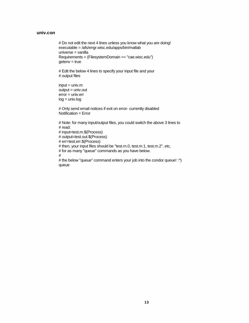
univ.con........................................................................................13

citizen.con ....................................................................................14

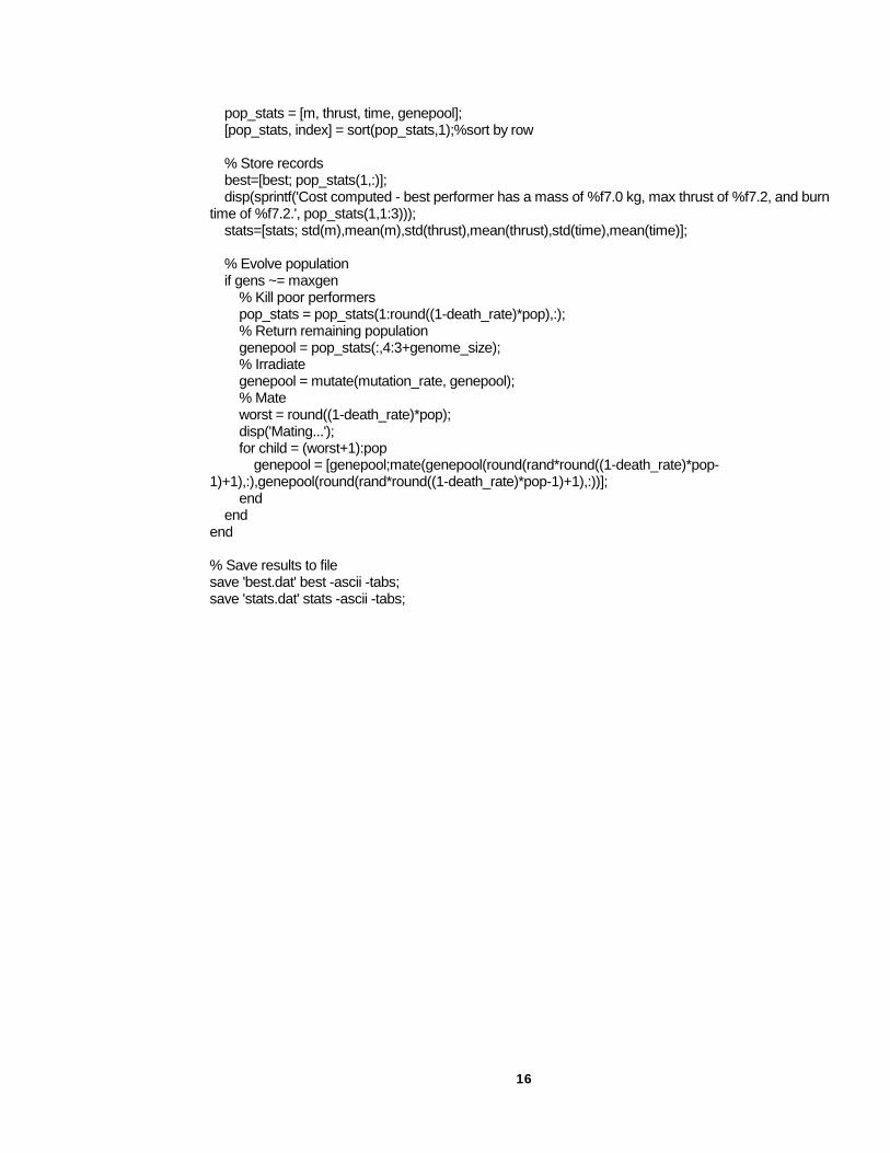
univ.m...........................................................................................15

find_cost.m...................................................................................17

cost.m...........................................................................................18

control_int.m.................................................................................20

write_citizens.m............................................................................21

citizen1.m (example citizen##.m file) ...........................................22

make_genepool.m .......................................................................23

phenome.m..................................................................................24

mate.m .........................................................................................25

mutate.m ......................................................................................26

f_aero.m.......................................................................................27

1

1.Introduction

Three months ago Dennis Tito marked the rekindling of the space industry by donating $20 million to the Russian Space Agency in exchange for a ten day trip aboard a Soyuz capsule

to the International Space Station – Alpha. The 50 years of the space program in the United States will soon become the largest corporate endeavor undertaken in any field. Conglomerates such as Boeing Corporation, Airbus, and Energia, in the United States, Europe, and Russia, respectively, already find themselves cooperating – and competing – with their own governments to launch satellites, experiments, and people, into the depths of the skies.

As we enter this era, there is a necessity to design the most efficient vehicle possible at as cheap a cost as possible. The current state of the art in launch vehicles combined with the demand makes the cost for a personal visit to space not only hard to pay, but an impossible competition with global interests. It costs $5,000 of payload for an astronaut to bring a thin magazine with to orbit. Even the cost to launch experimental packages can prove prohibitive to organizations that could improve life as we know it. There is a need to optimize launch vehicle performance.

The main goal of launch vehicle optimization is to increase the ratio of payload mass to launch vehicle mass well beyond the current state of the art – on the order of 5%. The two approaches to this are to minimize mass of structural components and to optimize the trajectory for reaching orbit. The former is the primary focus of industry at present. A recent renovation of the Space Shuttle’s external fuel tank replaced the fuel tank walls with a new Aluminum-Lithium alloy that weighs 1/3 less than the previous tank. Consequently, the shuttle’s cargo capacity was increased by 1 metric tonne – an outstanding accomplishment. The focus of this paper, though, will be on a topic assumed to be fully matured – launch vehicle trajectory.

The current state of the art uses a trajectory that is optimized for the defined parameters, but the number of parameters defined is of such small scope in order to use a Minimum Hamiltonian Ascent Trajectory Evaluation (MASTRE) derived algorithm, that there exists significant room for improvement – especially with the use of a high-performance, throttleable hybrid rocket engine. In order to develop the best thrust profile, the use of a genetic algorithm will be explored.

Second Stage

First Stage

150 kg Payload

Light Weight Composite Graincase

High Efficiency Nozzle

Ordnance-free staging

Failsafe Helium Pressurant

Advanced Alloy Oxygen Tank

Vortex Hybrid Rocket Engines

Optimized Nozzles

Figure 1: Zephyr-I Launch Vehicle design used for the genetic algorithm trajectory study.

2

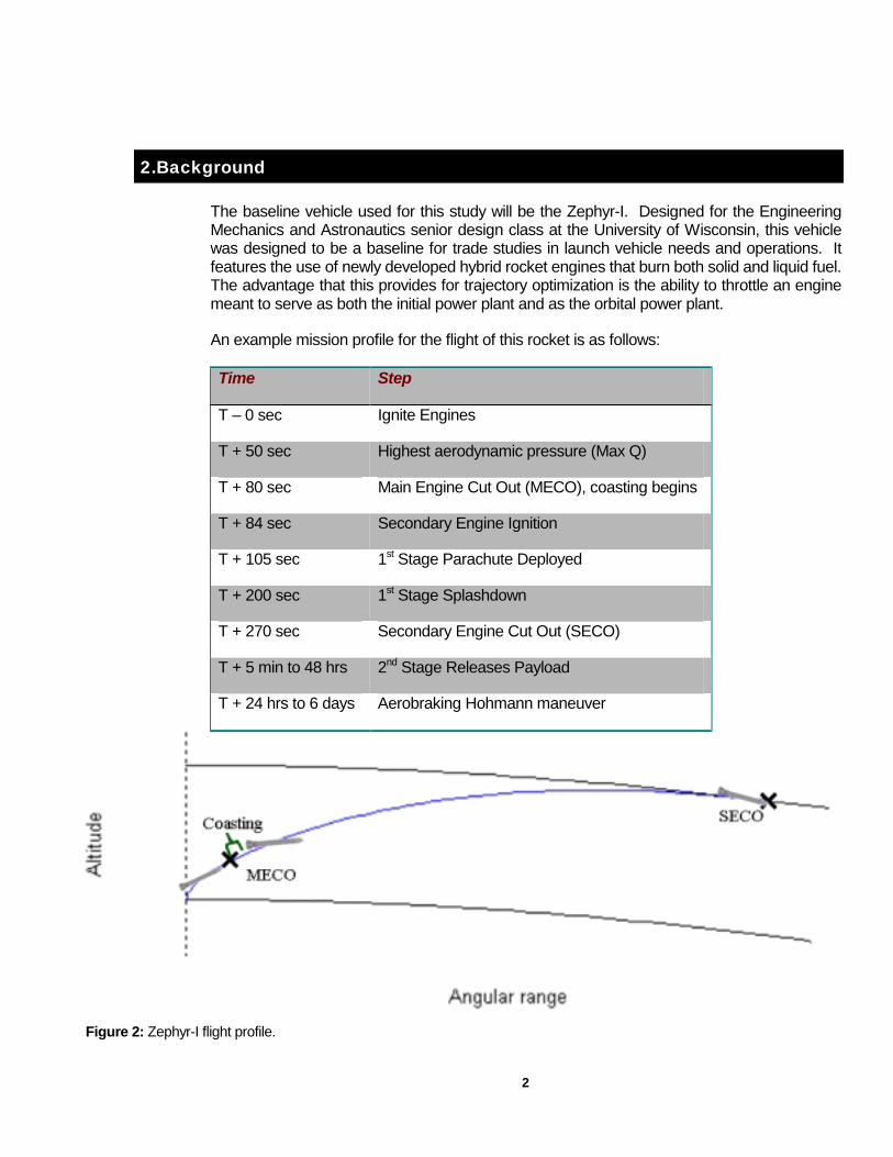
Figure 2: Zephyr-I flight profile.

2.Background

The baseline vehicle used for this study will be the Zephyr-I. Designed for the Engineering Mechanics and Astronautics senior design class at the University of Wisconsin, this vehicle was designed to be a baseline for trade studies in launch vehicle needs and operations. It features the use of newly developed hybrid rocket engines that burn both solid and liquid fuel. The advantage that this provides for trajectory optimization is the ability to throttle an engine meant to serve as both the initial power plant and as the orbital power plant.

An example mission profile for the flight of this rocket is as follows:

Time Step

T – 0 sec Ignite Engines

T + 50 sec Highest aerodynamic pressure (Max Q)

T + 80 sec Main Engine Cut Out (MECO), coasting begins

T + 84 sec Secondary Engine Ignition

T + 105 sec 1st Stage Parachute Deployed

T + 200 sec 1st Stage Splashdown

T + 270 sec Secondary Engine Cut Out (SECO)

T + 5 min to 48 hrs 2nd Stage Releases Payload

T + 24 hrs to 6 days Aerobraking Hohmann maneuver

3

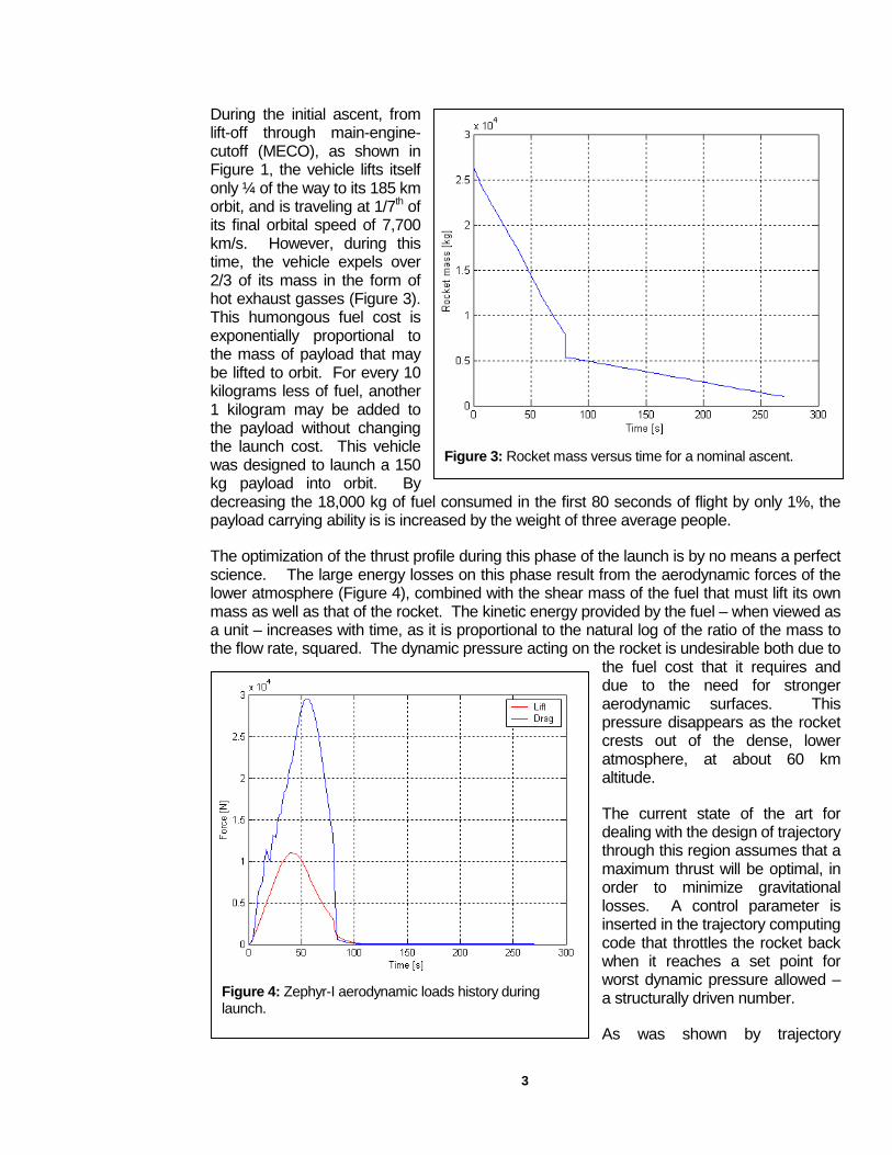
During the initial ascent, from lift-off through main-engine-cutoff (MECO), as shown in Figure 1, the vehicle lifts itself only ¼ of the way to its 185 km orbit, and is traveling at 1/7th of its final orbital speed of 7,700 km/s. However, during this time, the vehicle expels over 2/3 of its mass in the form of hot exhaust gasses (Figure 3). This humongous fuel cost is exponentially proportional to the mass of payload that may be lifted to orbit. For every 10 kilograms less of fuel, another 1 kilogram may be added to the payload without changing the launch cost. This vehicle was designed to launch a 150 kg payload into orbit. By decreasing the 18,000 kg of fuel consumed in the first 80 seconds of flight by only 1%, the payload carrying ability is is increased by the weight of three average people.

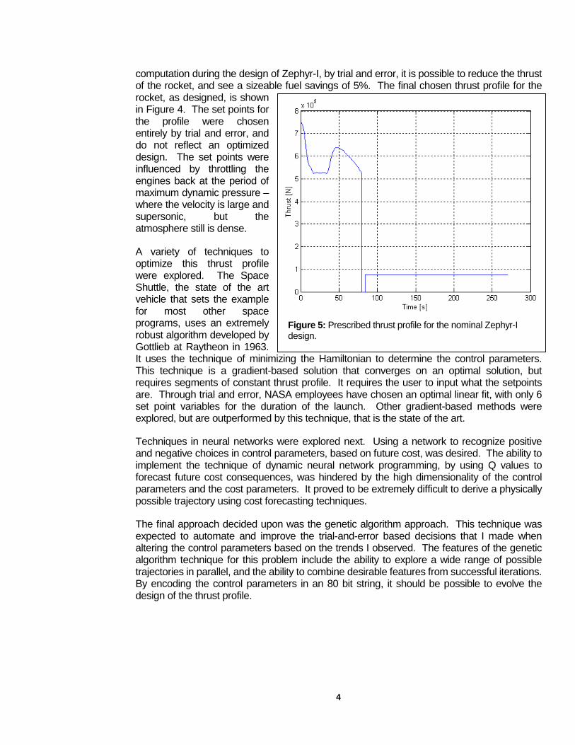
The optimization of the thrust profile during this phase of the launch is by no means a perfect science. The large energy losses on this phase result from the aerodynamic forces of the lower atmosphere (Figure 4), combined with the shear mass of the fuel that must lift its own mass as well as that of the rocket. The kinetic energy provided by the fuel – when viewed as a unit – increases with time, as it is proportional to the natural log of the ratio of the mass to the flow rate, squared. The dynamic pressure acting on the rocket is undesirable both due to

the fuel cost that it requires and due to the need for stronger aerodynamic surfaces. This pressure disappears as the rocket crests out of the dense, lower atmosphere, at about 60 km altitude.

The current state of the art for dealing with the design of trajectory through this region assumes that a maximum thrust will be optimal, in order to minimize gravitational losses. A control parameter is inserted in the trajectory computing code that throttles the rocket back when it reaches a set point for worst dynamic pressure allowed – a structurally driven number.

As was shown by trajectory

Figure 3: Rocket mass versus time for a nominal ascent.

Figure 4: Zephyr-I aerodynamic loads history during launch.

4

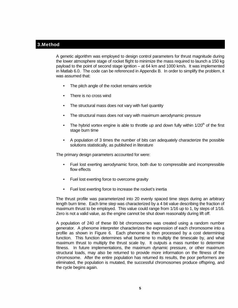
computation during the design of Zephyr-I, by trial and error, it is possible to reduce the thrust of the rocket, and see a sizeable fuel savings of 5%. The final chosen thrust profile for the rocket, as designed, is shown in Figure 4. The set points for the profile were chosen entirely by trial and error, and do not reflect an optimized design. The set points were influenced by throttling the engines back at the period of maximum dynamic pressure – where the velocity is large and supersonic, but the atmosphere still is dense.

A variety of techniques to optimize this thrust profile were explored. The Space Shuttle, the state of the art vehicle that sets the example for most other space programs, uses an extremely robust algorithm developed by Gottlieb at Raytheon in 1963. It uses the technique of minimizing the Hamiltonian to determine the control parameters. This technique is a gradient-based solution that converges on an optimal solution, but requires segments of constant thrust profile. It requires the user to input what the setpoints are. Through trial and error, NASA employees have chosen an optimal linear fit, with only 6 set point variables for the duration of the launch. Other gradient-based methods were explored, but are outperformed by this technique, that is the state of the art.

Techniques in neural networks were explored next. Using a network to recognize positive and negative choices in control parameters, based on future cost, was desired. The ability to implement the technique of dynamic neural network programming, by using Q values to forecast future cost consequences, was hindered by the high dimensionality of the control parameters and the cost parameters. It proved to be extremely difficult to derive a physically possible trajectory using cost forecasting techniques.

The final approach decided upon was the genetic algorithm approach. This technique was expected to automate and improve the trial-and-error based decisions that I made when altering the control parameters based on the trends I observed. The features of the genetic algorithm technique for this problem include the ability to explore a wide range of possible trajectories in parallel, and the ability to combine desirable features from successful iterations. By encoding the control parameters in an 80 bit string, it should be possible to evolve the design of the thrust profile.

Figure 5: Prescribed thrust profile for the nominal Zephyr-I design.

5

3.Method

A genetic algorithm was employed to design control parameters for thrust magnitude during the lower atmosphere stage of rocket flight to minimize the mass required to launch a 150 kg payload to the point of second stage ignition – at 64 km and 1000 km/s. It was implemented in Matlab 6.0. The code can be referenced in Appendix B. In order to simplify the problem, it was assumed that:

• The pitch angle of the rocket remains verticle

• There is no cross wind

• The structural mass does not vary with fuel quantity

• The structural mass does not vary with maximum aerodynamic pressure

• The hybrid vortex engine is able to throttle up and down fully within 1/20th of the first stage burn time

• A population of 3 times the number of bits can adequately characterize the possible solutions statistically, as published in literature

The primary design parameters accounted for were:

• Fuel lost exerting aerodynamic force, both due to compressible and incompressible flow effects

• Fuel lost exerting force to overcome gravity

• Fuel lost exerting force to increase the rocket’s inertia

The thrust profile was parameterized into 20 evenly spaced time steps during an arbitrary length burn time. Each time step was characterized by a 4 bit value describing the fraction of maximum thrust to be employed. This value could range from 1/16 up to 1, by steps of 1/16. Zero is not a valid value, as the engine cannot be shut down reasonably during lift off.

A population of 240 of these 80 bit chromosomes was created using a random number generator. A phenome interpreter characterizes the expression of each chromosome into a profile as shown in Figure 6. Each phenome is then processed by a cost determining function. This function determines what burntime to multiply the timescale by, and what maximum thrust to multiply the thrust scale by. It outputs a mass number to determine fitness. In future implementations, the maximum dynamic pressure, or other maximum structural loads, may also be returned to provide more information on the fitness of the chromosome. After the entire population has returned its results, the poor performers are eliminated, the population is mutated, the successful chromosomes produce offspring, and the cycle begins again.

6

In order to take advantage of the highly parallel nature of this algorithm, and to accommodate the 10 to 30 minutes of CPU time that it takes to compute cost, this program was implemented using the Computer Science Department’s Condor High-Throughput Computing software. The time cost is a consequence of the need for the control integration and cost computing codes to iteratively find a solution.

A universe control code was submitted to condor first. It begins by writing a status file to the directory for its “citizens” to see, and then writes the citizen control files, based on the size of the population. It then looped for the preset number of generations, calling the cost finding algorithm at the beginning of each loop. The call to the cost finding algorithm starts a script with a loop that will cycle until all citizens have found the cost for the current iteration’s chromosomes. This is signaled by the citizens writing the new generation number to their own status file. The citizens are initialized, after written by the universe control code, by submitting a second job to condor, queuing all citizen files. These files loop continually looking for the status of the universe to change. Then they process the new population. By this method, the code may be run for 50 iterations in a period of 1500 minutes maximum, or approximately 1 day. In that day, the trajectory will be integrated and converged upon to an unprecedented level, based on a population of 12,000 evolved chromosomes.

Figure 6: Unscaled thrust profiles for test citizens 1 through 5.

7

4.Results

The program shows great promise to produce results of significant academic interest. Unfortunately, a successful run was never completed due to two reasons.

First, there was a steep learning curve for implementing this technique in Condor. Determining the hand shaking system via flags in files took significant time to implement successfully – especially with continual upgrades to the Condor system. During the lifetime of this project, a password protection scheme was implemented on Condor that prevented my original intention to control Condor through a MatLab script. Also in that time, Condor underwent unpublished downtimes that appeared in the form of incomprehensible error messages that wasted large amounts of time.

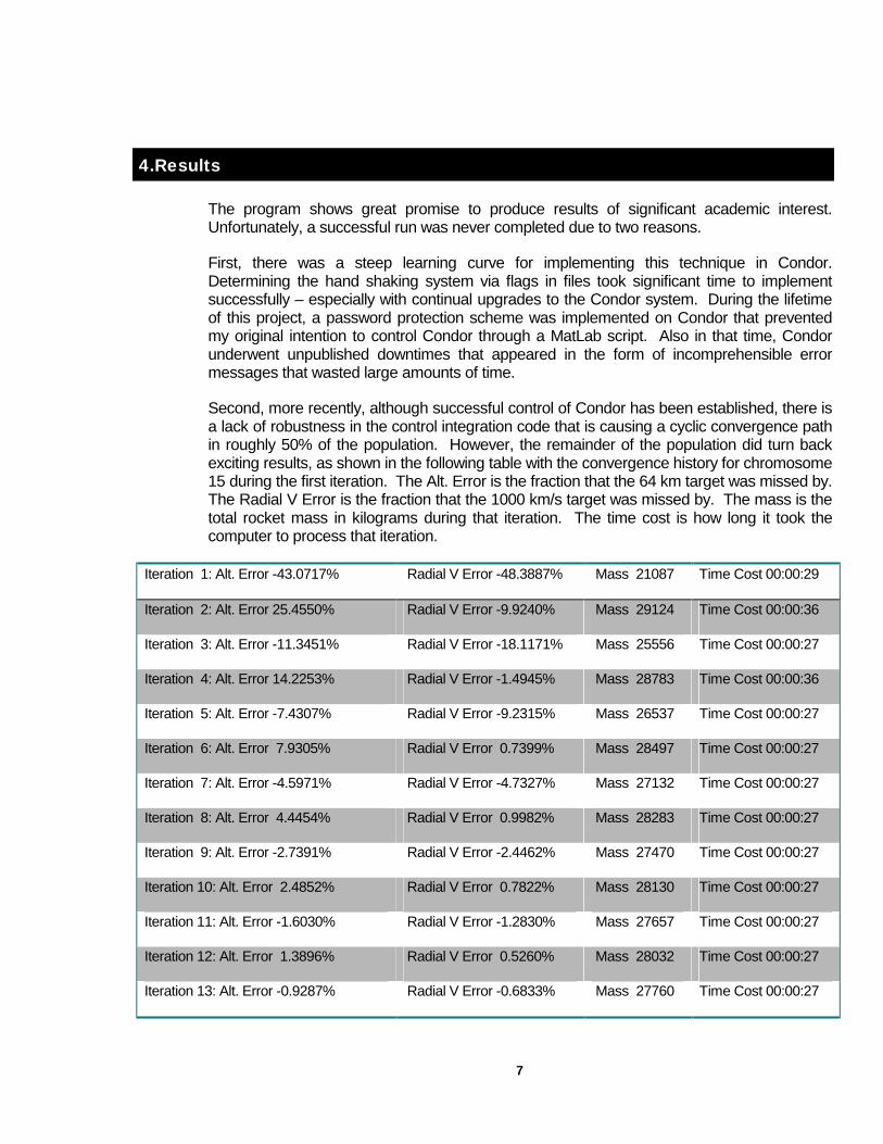
Second, more recently, although successful control of Condor has been established, there is a lack of robustness in the control integration code that is causing a cyclic convergence path in roughly 50% of the population. However, the remainder of the population did turn back exciting results, as shown in the following table with the convergence history for chromosome 15 during the first iteration. The Alt. Error is the fraction that the 64 km target was missed by. The Radial V Error is the fraction that the 1000 km/s target was missed by. The mass is the total rocket mass in kilograms during that iteration. The time cost is how long it took the computer to process that iteration.

Iteration 1: Alt. Error -43.0717% Radial V Error -48.3887% Mass 21087 Time Cost 00:00:29

Iteration 2: Alt. Error 25.4550% Radial V Error -9.9240% Mass 29124 Time Cost 00:00:36


Iteration 4: Alt. Error 14.2253% Radial V Error -1.4945% Mass 28783 Time Cost 00:00:36


Iteration 6: Alt. Error 7.9305% Radial V Error 0.7399% Mass 28497 Time Cost 00:00:27








8



























9






10

5.Conclusion

There is a significant need in the aerospace industry to develop optimized launch vehicle trajectories in lieu of previously accepted non-optimal assumptions. The potential for increase in profit from such an improvement is in the range of billions of dollars. It has the potential to triple or quadruple the cargo capacity of current and future launch vehicles, in turn cutting the transportation cost by the same number of times.

The method developed in this paper, and provided in the code in Appendix B, will be capable of converging on an evolved solution that will allow the baseline rocket design to outperform any comparable rocket on the market.

For future work, to be completed in the next several weeks, the genetic algorithm will be debugged on the Condor system, after the CAE network returns from the planned one week down time. A final code and appendum will be submitted at that time, along with what is expected to be some publicly meaningful results.

This technique will allow for the survival of the fittest trajectory profile out of a sample population that is 50 generations old, and has had a total of 12,000 members evolve, crossover, mutate and pass on the successful traits to the next generation.

11

Appendix A – References

Anderson, John D. Jr. Fundamentals of Aerodynamics 2nd Ed.. McGraw-Hill, New York. 1991.

Anderson, M.B., et. al. “Missile Aerodynamic Shape Optimization Using Genetic Algorithms”. AIAA Journal. Vol 37 No 5, Sept-Oct 2000.

Bowles, J. Near Optimal Operation of Dual-Fuel Launch Vehicles. AIAA Atmospheric Flight Mechanics Conference: San Diego, CA, 1996.

Bilstein, R., Stages to Saturn. Washington DC: National Aeronautics and Space Administration, 1980.

Hu, Yu Hen. Introduction to Neural Networks Course Notes. University of Wisconsin – Madison, 1999.

Koelle, H., Handbook of Astronautical Engineering. New York: McGraw-Hill Book Company, Inc., 1961.

Leitmann, George. Optimization Techniques With Applications to Aerospace Systems. Academic Press, New York. 1962.

Lyons, J. T. Minimum Hamiltonian Ascent Trajectory Evalaution (MASTRE) Program (update to automatic flight trajectory design, performance prediction, and vehicle sizing for support of shuttle and shuttle derived vehicles) engineering manual: final report. Marshall Space Flight Center, AL : Marshall Space Flight Center, National Aeronautics and Space Administration, 1993.

Scipio, Albert L. Structural Design Concepts. Office of Technology Utilization, National Aeronautics and Space Administration. Washington, D.C. 1967.

Steve, previous EMA 569 rocket design semester report, 2000.

Vinson, J. The Behavior of Sandwich Structures of Isotropic and Composite Materials. Lancaster: Technomic, 1993 and 1999.

Wertz, James R. and Larson, Wiley J. Space Mission Analysis and Design. Microcosm Press, El Segundo, CA, 1999.

Schoonover, P.L., et. al. “Application of a Genetic Algorithm to the Optimization of Hybrid Rockets”. AIAA Journal. Vol 37 No 5, Sept-Oct 2000.

12

Appendix B – Code

The following segments of code were written exclusively for the ECE 539 term project. Any function calls in “m” files not inherent to the Unix version of MatLab 6.0 may be found either in the NT version of MatLab 6.0 library or in the senior design report for Engineering Mechanics and Astronautics, 2001.

The first two pages of code are the scripts to submit jobs to the Condor High-Throughput computing system. The remainder are MatLab 6.0 script files.

13

univ.con

# Do not edit the next 4 lines unless you know what you are doing! executable = /afs/engr.wisc.edu/apps/bin/matlab universe = vanilla Requirements = (FilesystemDomain == "cae.wisc.edu") getenv = true # Edit the below 4 lines to specify your input file and your # output files input = univ.m output = univ.out error = univ.err log = univ.log # Only send email notices if exit on error- currently disabled Notification = Error # Note: for many input/output files, you could switch the above 3 lines to # read: # input=test.m.$(Process) # output=test.out.$(Process) # err=test.err.$(Process) # then, your input files should be "test.m.0, test.m.1, test.m.2", etc, # for as many "queue" commands as you have below. # # the below "queue" command enters your job into the condor queue! :^) queue

14

citizen.con

# Do not edit the next 4 lines unless you know what you are doing! executable = /afs/engr.wisc.edu/apps/bin/matlab universe = vanilla Requirements = (FilesystemDomain == "cae.wisc.edu") getenv = true # Edit the below 4 lines to specify your input file and your # output files #input = citizen.m #output = univ.out #error = univ.err #log = univ.log # Only send email notices if exit on error- currently disabled Notification = Error # Note: for many input/output files, you could switch the above 3 lines to # read: input=citizen$(Process).m output=citizen$(Process).out err=citizen$(Process).err log=citizen$(Process).log # then, your input files should be "test.m.0, test.m.1, test.m.2", etc, # for as many "queue" commands as you have below. # # the below "queue" command enters your job into the condor queue! :^) queue 19

15

univ.m

% Universe Control Code % Main Trajectory GA Program % Written by Gabe Hoffmann, 5/18/2001 % Clear old generations !rm citizen*.dat -f !rm citizen*.m -f % Set universe dimensions disp('Starting the universe'); thrust_level_bits = 2; time_bits = 3; genome_size = thrust_level_bits*time_bits; pop = 3*genome_size; % Set generational probabilities death_rate = 0.5; mutation_rate = 0.02; % Make gene pool disp('Making genepool'); genepool = make_genepool(genome_size,pop); % Set number of generations to compute maxgen = 3; % Initialize results storing matrices best = []; stats = []; % Prevent citizens from iterating until ready gens = 0; save('univ_stat.dat','gens','-ascii'); % Create files to submit as citizens disp('Creating citizens'); write_citizens(pop,maxgen); % Iterate through all generations for gens = 1:maxgen disp(sprintf('Starting generation %i',gens)); % Update genepool info for citizens to read save('population.dat','genepool','-ascii'); % Queue citizens to compute when called by increasing iteration flag save('univ_stat.dat','gens','-ascii'); % Retrieve performance characteristics of each citizen when done iterating [m, thrust, time] = find_cost(genepool,gens); % Sort by performance

16

pop_stats = [m, thrust, time, genepool]; [pop_stats, index] = sort(pop_stats,1);%sort by row % Store records best=[best; pop_stats(1,:)]; disp(sprintf('Cost computed - best performer has a mass of %f7.0 kg, max thrust of %f7.2, and burn time of %f7.2.', pop_stats(1,1:3))); stats=[stats; std(m),mean(m),std(thrust),mean(thrust),std(time),mean(time)]; % Evolve population if gens ~= maxgen % Kill poor performers pop_stats = pop_stats(1:round((1-death_rate)*pop),:); % Return remaining population genepool = pop_stats(:,4:3+genome_size); % Irradiate genepool = mutate(mutation_rate, genepool); % Mate worst = round((1-death_rate)*pop); disp('Mating...'); for child = (worst+1):pop genepool = [genepool;mate(genepool(round(rand*round((1-death_rate)*pop-1)+1),:),genepool(round(rand*round((1-death_rate)*pop-1)+1),:))]; end end end % Save results to file save 'best.dat' best -ascii -tabs; save 'stats.dat' stats -ascii -tabs;

17

find_cost.m

function [m, thrust, time] = find_cost(population,iteration) [rows,cols] = size(population); done_growing = 0;%initialize to false while done_growing == 0 done_growing = 1; for person = 1:rows fname = ['citizen', int2str(person), '.dat']; fid = fopen(fname,'r'); if fid<0 done_growing = 0; else if str2num(fgetl(fid))<iteration done_growing = 0; end end fclose(fid); end end m = []; thrust = []; time = []; for person = 1:rows disp(person); fname = ['citizen', int2str(person), '.dat']; fid = fopen(fname,'r'); tmp = fgetl(fid); tmp = fgetl(fid); [str_m rem] = strtok(tmp); [str_thrust str_time] = strtok(rem); m = [m;str2num(str_m)]; thrust = [thrust;str2num(str_thrust)]; time = [time;str2num(str_time)]; fclose(fid); end

18

cost.m

%%%%%%%%%%%%%%%%%%%%%%%%%%%%%%%%%%%%%%%%%%% % Filename: compute.m % Purpose: Primary excecutable % Called by: User % Modified: 5/12/2001, Gabe Hoffmann % % compute.m is the excecutable file for the % trajectory integration and orbital % convergence algorithm. %%%%%%%%%%%%%%%%%%%%%%%%%%%%%%%%%%%%%%%%%%% function [m,T_max,burn_time] = cost(chromosome,person) %%%%%%%%%%%%%%%%%%%%%%%%%%%%%%%%%%%%%%%%%%% % Initialize variables and set options %%%%%%%%%%%%%%%%%%%%%%%%%%%%%%%%%%%%%%%%%%% % Clear all variables and set output format %clear; format long g; % Load constants constants; atm_model; % Load input parameters from input_params.m input_params; begin_tot = now; begin = now; disp(sprintf('Started iterating at %s',datestr(begin, 'HH:MM:SS PM'))); %%%%%%%%%%%%%%%%%%%%%%%%%%%%%%%%%%%%%%%%%%% % Run orbital convergence until tolerances % are met %%%%%%%%%%%%%%%%%%%%%%%%%%%%%%%%%%%%%%%%%%% go_on = 0; % While loop flag i = 0; % Iteration counter % Loop until radius, radial velocity, and angular velocity % meet tolerences defined in input_params.m T_points1 = phenome(chromosome); fname = ['citizen', int2str(person),'.nfo']; while (go_on == 0)*(i < 200) % Increment index i = i + 1; % Assume that tolerences will be met go_on = 1; % Run integration (see control_integration.m) [t,radius,radial_vel,radial_accel,mass,masses] = control_int(m,Isp,r0,T_max,burn_time,T_points1);

19

% Extract key values from returned data rf = radius(length(radius)); vrf = radial_vel(length(radial_vel)); total_mass = masses(1,1); m(1,1)=masses(1,1); % Store key values in results matrix results(i,1:3) = [(rf - ro)/(ro-re_m),(vrf-vf)/vf,total_mass]; fid = fopen(fname,'a'); if fid<0 % do nothing; error else fprintf(fid,'Iteration %2i: Alt. Error %7.4f%%, Radial V Error %7.4f%%, Mass %6.f, Time Cost %s\n'... ,i,results(i,1)*100,results(i,2)*100,results(i,3), datestr(now-begin, 'HH:MM:SS')); fclose(fid); end; begin = now; % Based upon how the results fail to hit target values, adjust: % - Note: these parameter modification functions were contructed by % inspection and can be modified to increase or decrease % how quickly the convergence occurs. eta1 = 1; eta2 = 0.6; eta3 = 0.6; if abs((rf - ro)/(ro - re_m)) > radius_tolerance burn_time = burn_time*(1+eta1*(ro - rf)/(ro - re_m)); go_on = 0; end if abs(vrf-vf)/vf > radial_velocity_tolerance T_max=T_max*(1+eta2*(vf-vrf)/vf); go_on = 0; end end %Output key data for user inspection disp(sprintf('Converged at %s, time cost is %s',datestr(now, 'HH:MM:SS PM'), datestr(now-begin_tot, 'HH:MM:SS'))); disp(sprintf('Final Altitude: %.2f km, Desired Altitude: %.2f km',(radius(length(radius))-re*1000)/1000,(ro-re*1000)/1000)); disp(sprintf('Final Radial Velocity: %.2f m/s',radial_vel(length(radial_vel)))); disp(sprintf('Total Rocket Mass: %.0f kg', masses(1,1))); disp(sprintf('Required 1st Stage Fuel: %.0f kg, Required 2nd Stage Fuel: %.0f kg',m(1,1)-m(1,2)-m(2,1), m(2,1)-m(2,2))); if i>=200 m = 10e10;%eliminate gene else m = m(1,1); end

20

control_int.m

%%%%%%%%%%%%%%%%%%%%%%%%%%%%%%%%%%%%%%%%%%% % Filename: control_int.m % purpose: integrates trajectory given % key input parameters % % control_integration.m integrates the % rocket trajectory given the input % parameters, which are listed below. %%%%%%%%%%%%%%%%%%%%%%%%%%%%%%%%%%%%%%%%%%% function [t,radius,radial_vel,radial_accel,mass,masses] = control_integration(m,Isp,r0,T_max,burn_time,T_points) global T_points_stage; global Isp_stage; constants; T_points_stage = [burn_time * T_points(1,:); T_max * T_points(2,:)]; Isp_stage = Isp; % iterate on first stage until mass at end of burn equals desired mass based on % first stage strucure mass and second stage mass go_on = 0; it = 0; while (go_on == 0)&(it<400); % run integration using ode45 and equations_of_motion [t,y] = ode45('eq_of_motion',[0,burn_time],[r0,0,m(1,1)]); % extract mass from results mass = y(:,3); % if mass incorrect, change and run again, otherwise, exit loop if abs((mass(length(mass)) - (m(1,2)+m(2,1)))/(m(1,2)+m(2,1))) > 0.001; m(1,1) = abs(m(1,1) + (m(1,2) + m(2,1) - mass(length(mass)))); else go_on = 1; end end % extract remaining details from first stage integration radius = y(:,1); radial_vel = y(:,2); % Calculate acceleration plots: radial_accel = diff(radial_vel) ./ diff(t); masses = mass;

21

write_citizens.m

function write_citizens(pop,gen_max) output = 0; mname = ['citizen0.m']; save(mname,'output','-ascii'); for person = 1:pop disp(sprintf('Person %i',person)); output = 0; fname = ['citizen', int2str(person), '.dat']; mname = ['citizen', int2str(person), '.m']; save(fname,'output','-ascii'); fid=fopen(mname,'w'); fprintf(fid,'gen = 1;\n'); fprintf(fid,'while gen<=%i\n',gen_max); fprintf(fid,'\tidle = 1;\n'); fprintf(fid,'\twhile idle == 1\n'); fprintf(fid,'\t\tfname = \''univ_stat.dat\'';\n'); fprintf(fid,'\t\tfid = fopen(fname,\''r\'');\n'); fprintf(fid,'\t\tif fid>=0\n'); fprintf(fid,'\t\t\tif str2num(fgetl(fid))==gen\n'); fprintf(fid,'\t\t\t\tidle=0;\n'); fprintf(fid,'\t\t\tend;\n'); fprintf(fid,'\t\tend;\n'); fprintf(fid,'\t\tfclose(fid);\n'); fprintf(fid,'\tend;\n'); fprintf(fid,'\tfname = \''population.dat\'';\n'); fprintf(fid,'\tfid = fopen(fname,\''r\'');\n'); fprintf(fid,'\tline = 0;\n'); fprintf(fid,'\twhile line<%i\n',person); fprintf(fid,'\t\tinput = fgetl(fid);\n'); fprintf(fid,'\t\tline = line+1;\n'); fprintf(fid,'\tend\n'); fprintf(fid,'\tchromosome = str2num(input);\n'); fprintf(fid,'\t[m, thrust, time] = cost(chromosome,%i);\n',person); fprintf(fid,'\tfname = [\''citizen\'', int2str(%i), \''.dat\''];\n',person); fprintf(fid,'\tfid = fopen(fname,\''w\'');\n'); fprintf(fid,'\tfprintf(fid,\''%%i\\n%%f\\t%%f\\t%%f\\t\'',gen, m, thrust, time);\n'); fprintf(fid,'\tfclose(fid);\n'); fprintf(fid,'\tgen = gen+1;\n'); fprintf(fid,'end;'); fclose(fid); end

22

citizen1.m (example citizen##.m file)

gen = 1; while gen<=3 idle = 1; while idle == 1 fname = 'univ_stat.dat'; fid = fopen(fname,'r'); if fid>=0 if str2num(fgetl(fid))==gen idle=0; end; end; fclose(fid); end; fname = 'population.dat'; fid = fopen(fname,'r'); line = 0; while line<1 input = fgetl(fid); line = line+1; end chromosome = str2num(input); [m, thrust, time] = cost(chromosome,1); fname = ['citizen', int2str(1), '.dat']; fid = fopen(fname,'w'); fprintf(fid,'%i\n%f\t%f\t%f\t',gen, m, thrust, time); fclose(fid); gen = gen+1; end;

23

make_genepool.m

function pool = make_genepool(bits,pop) pool = (rand(pop,bits)>0.5);

24

phenome.m

function T_points = phenome(chromosome) % number of bits for thrust level determination T_res = 2; % number of time steps [rows,cols]=size(chromosome); time_res = cols/T_res; T_points = zeros(2,time_res); T_points(1,:) = 0:1/(time_res-1):1; for step = 1:time_res T_points(2,step) = binvec2dec(chromosome((step-1)*T_res+1:step*T_res)); end T_points(2,:) = (T_points(2,:)+1)/(2^T_res);

25

mate.m

function chrom = mate(chrom1, chrom2) flip = (rand(size(chrom1))<0.5); flip = [flip;xor(flip,1)]; chrom = sum(flip.*[chrom1;chrom2]);

26

mutate.m

function population = mutate(mutation_rate, population) population = xor(population,(rand(size(population))<=mutation_rate));

27

f_aero.m

function [F_aero_r, F_aero_alpha, F_lift, F_drag,... F, D_v, L, D_p, D_b, q] = f_aero(altitude, velocity) input_params atm_model %%%%%%%%%%%%%%%%%%%%%%%%%%%%%%%%%%%%%%%%%%% % define drag parameters %%%%%%%%%%%%%%%%%%%%%%%%%%%%%%%%%%%%%%%%%%% % Interpolate temperature (K) from data temperature = spline(atm(:,1),atm(:,2),altitude); % Interpolate pressure (Pa) from data pressure = spline(atm(:,1),atm(:,4),altitude); % Interpolate density (kg/m^3) from data density = spline(atm(:,1),atm(:,5),altitude); % Speed of sound (m/s) a = 20.047*sqrt(temperature); % Mach number M = velocity/a; % Viscosity mu = 1.8*10^-5; % Reynolds number Re = density.*velocity*L_rocket/mu; % Dynamic pressure q = 1/2*density.*velocity.^2; % Friction factor C_f = 0.074./(Re+0.0001).^0.2*(1+0.5/rat1); % Viscous drag D_v = C_f.*S_surface.*q; % Coefficient of lift C_L = 0; % Aerodynamic Pressure Force F = 0; % Lift due to pressure L = 0; % Pressure drag D_p = 0; % Base drag D_b = 2*r_eff*0.029*q/sqrt(0.2); % Totalling the drag and lift F_lift = L; F_drag = D_v; % Conversion into radial and axial forces F_aero_r = -F_drag; F_aero_alpha = 0;

Launch Vehicle Thrust...

Documents

Transcript of Launch Vehicle Thrust...