Rend. Sem. Mat. Univ. Poi. Torino Voi. 51, 3 (1993)

Num. Meth. Astr. Cosm.

L. Moscardini

COSMOLOGICAL PARTICLE-MESH N-BODY SIMULATTONS AND THE ROLE OF INITIAL CONDITIONS

Abstract. We present a description of the numerical techniques underlying N-

body siinulations. They have been introduced in order to solve the problem of

the gravitational interaction of a large set of particles. We show how they work

in cosmological configurations. In particular we discuss two different schemes: the

particle-particle and particle-mesh methods. We also present the algorithm used in

order to set the initial conditions for the particles, given the distribution and power

spectrum of the density fluctuations. The Zel'dovich approximation, which is the

tool used for this goal, is also presented. The algorithms for Gaussian and some

non-Gaussian distributions are shown in more details. The role of different initial

conditions in the study of large-scale structure formation is discussed, presenting

some results from TV-body simulations.

1. Introduction

Numerical simulations have become in the last years one of the most effective tools to study and solve astrophysical problems. The calculation of the mutuai gravitational interaction of a large set of particles is a problem which is not possibie to solve only with analytical techniques. Therefore this case is a good example of a problem where the computer help is fundamental.

In the last 20 years, technological progress has given to the scientific community computational facili ties with largely improved speed and memory allocation. In the same time a series of numerical techniques has been developed, giving the possibility of facing wider and more complicate problems.

For these reasons, the study of the formation and evolution of cosmological structures, analyzed only with analytical approaches until the half of the 70's, is now mainly

250 L. Moscardini

based on numerical simulations. In this field they substitute the laboratory experiments which are in practice impossible for cosmology: in fact this science has to face with the problems deriving from the existence of a unique universe and from the large limitations and uncertainties due to observational results which cover a very short time range compared to the age of the universe.

The pian of this paper is as follows. In Section 2 we review the TV-body techniques, presenting the equations of the model and the details of two possible methods to solve them: the particle-particle (PP) and the particle-mesh (PM) method; the conservation tests used in order to evaluate the accuracy of a code are also introduced. In Section 3 we deal with the problem of setting initial conditions for TV-body simulations in cosmological conflgurations: the method, based on the Zel'dovich approximation, is studied in the context of botri Gaussian and non-Gaussian distributions for the density fluctuations field. Some results obtained from the study of large-scale structure formation are also sketched.

2. N-body simulations

2.1. Model equations

In order to write the equations of motion determining the gravitational phenomena on large scales it is necessary to choose an underlying cosmological model. In the frame of General Relativity, a possible and usuai choice is given by Friedmann-Lemaitre models with zero cosmological Constant.

On the scales where homogeneity and isotropy hold, a relatively small region is a fair sample of the whole universe: in this case it is possible to follow the Newtonian approach plus suitable changes due to General Relativity.

Since the observations show that the universe is expanding, it is convenient to make use of comoving spatial coordinates defined as x = r/a(t), where r*is the proper position and a(t) is the expansion factor, which follows the Hubble law: à = Ha, where II is the Hubble Constant.

The equations of motion that describe the evolution of each object, assumed with unit mass are

(1) ù = F = V<i),

(2) ?±=i?,

where the gravitational field is given by Poisson equation

(3) V2(f> = 47rGp(rìt).

Cosmological Particle-Mesh N-Body Simulations 251

In comoving coordinates, the previous equations read (more details in Peebles 1980)

(4) x — v

(5) ÌJ=-2Hv-V(j>/a2

(6) V2<j> = 4TrG[p(rìt)-p] = 47rGp6,

where ~p is the mean density and 6 = p/~p — 1 is the density contrast.

2.2. The Particle-Particle method

This is the simplest possible method because it makes direct use of the equations of motion following from the Newton's gravitational law. In this approach the forces on each particle are directly calculated by accumulating the contributions of ali remaining particles.

At each time-step At the following operations are performed:

a) clearing of force accumulators: Fi = 0 for i = 1 , . . . , Np, where A ,̂ is number of particles;

b) accumulation of the forces between ali Np(Np — 1) pairs of particles: JFy oc rriimj/r2j, where r̂ - is the distance between two particles and mi, m7- are their mass:

•fi ~ fi ~T fij j

f 3 = Fj + fio '

c) integration of the equations of motion in order to obtain the updated velocities Vi and positions XÌ of the particles:

x?ew = xfd + vi • At .

d) updating of time counter: t = t + At.

Even if writing a numerical algorithm for this method is extremely easy, its computational cost is quite large, being proportional to NP(NP - 1): this fact forbids its application to problems with a large number of particles (in practice Np^> IO4).

If the standard scheme of the PP method is modified by introducing a different time-step for each particle (Aarseth 1971), the updating of the force contribution for the more distant particles is calculated with smaller frequency: this gives of course a useful reduetion of the computational time, allowing the application of PP methods to a larger number of particles (up to Np ~ IO5). In any case, each time-step with the PP method, applied to a problem with IO5 particles on a parallel/vector processor (0.1//s per operation), requires approximately 1 hour of CPU time!

In PP methods a fundamental problem in the calculation of the forces is their divergence at small distance. In order to avoid this it is necessary to reduce the impact

252 L. Moscardini

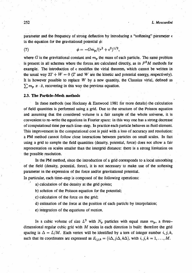
parameter and the frequency of strong deflection by introducing a "softening" parameter e in the equation for the gravitational potential </>:

(7) ^ - G m p / ( r 2 + e2)1/2,

where G is the gravitational Constant and mp the mass of each particle. The same problem is present in ali schemes where the forcesare calculated directly, as in P3M methods for example. The introduction of e modifìes the virial theorem, which cannot be written in the usuai way 2T + W = 0 (T and W are the kinetic and potential energy, respectively). It is however possible to replace W by a new quantity, the Clausius virial, deflned as ^2 mp x • x, recovering in this way the previous equation.

2.3. The Particle-Mesh methods

In these methods (see Hockney & Eastwood 1981 for more details) the calculation of field quantities is performed using a grid. Due to the structure of the Poisson equation and assuming that the considered volume is a fair sample of the whole universe, it is convenient to re-write the equations in Fourier space: in this way one has a strong decrease of computational time per each time-step. In practice each particle behaves as fluid element. This improvement in the computational cost is paid with a loss of accuracy and resolution: a PM method cannot follow dose interactions between particles on small scales. In fact using a grid to sample the field quantities (density, potential, force) does not allow a fair representation on scales smaller than the intergrid distance: there is a strong limitation on the possible resolution.

In the PM method, since the introduction of a grid corresponds to a locai smoothing of the field (density, potential, force), it is not necessary to make use of the softening parameter in the expression of the force and/or gravitational potential.

In particular, each time-step is composed of the following operations:

a) calculation of the density at the grid points;

b) solution of the Poisson equation for the potential;

e) calculation of the force on the grid;

d) estimation of the force at the position of each particle by interpolation;

e) integration of the equations of motion.

In a cubie volume of size L3 with Np particles with equal mass mp, a three-dimensional regular cubie grid with M nodes in each direction is built: therefore the grid spacing is A = L/M. Each vertex will be identified by a tern of integer number i,j, k, such that its coordinates are expressed as Xijìk = (*A, jA, /cA), with i,jyk = 1 , . . . , M.

Cosmological Particle-Mesh N-Body Simulations 253

• Density calculation

The particle mass decomposition at the grid nodes is one of the criticai points for the PM method, both for resolution and computational cost.

The mass density p at the grid point Xijtk can be written as

(8) p(xiJtk) = mpM3J2W(sài),

1=1

where W is a suitable interpolation function and Sòci = xi — XÌJ^ is the displacement between the position of the particle / and the considered grid point.

The choice of W is related to the goodness of the required approximation: of course the higher the number of grid points involved in the interpolation, the better the approximation. In higher dimensions it is possible to write the function W as product of more functions, depending only on the displacement in one dimension, i.e. Wi.j.fc = WÌ WJ wk.

In order of increasing resolution, the interpolation functions are:

(NGP) "nearest-grid-point":

in this case the mass of each particle is completely assigned only to the nearest grid point; the density shows therefore a discontinuity every time a particle crosses the grid border. The interpolation function reads

(9) WÌ = 1, M\6XÌ\<-\

(CIC) "cloud-in-cell":

the mass of each particle is assigned to two (23 = 8 in three-dimensional case) nearest points in an inversely proportional way with respect to its distànce from the grid point: in this way the density varies with continuity when a particle crosses the celi border, even if its gradient is stili discontinuous. The interpolation function in this case can be written as:

(10) WÌ = 1 - M\6XÌ\, M\6XÌ\ < 1;

(TSC) "triangular-shaped-cell":

the mass decomposition involves three (33 = 27 in 3-D) nearest grid points. In this way also the density gradient is continuous during the celi border crossing; on the contrary the second derivative will be stili discontinuous. The interpolation function can

254 L. Moscardini

be expressed as:

%-M26Xi2, M\6XÌ\ < £ ;

(11) Wi= ^ 11 3 M|<fa;| , ì <M|&C<| < § .

Extensions to higher orders are of course possible: they would show gradually continuous derivatives of higher orders. Because of the increasing number of involved points, the resulting interpolation would be better but the computational cost would largely increase.

The same interpolation schemes have to be used in order to obtain the components of the force on each particle, while conserving momentum: in this case

M

(12) Fx(xl) = mp ] T W(6xl)Fx(a!iìjtk) i,j,k=l-

M

(13) Fv(Sl) = mp £ W(,62l)Fy@iJ,h) i,j,k=l

M

(14) Fz(xl) = mp Y, W(8^)Fz(xiìjìk).

• Poisson equation

The Poisson equation [Eq.(3)] becomes much easier to solve introducing suitable Fast Fourier Trans for ms (FFT). Since it is possible and convenient to use periodic boundary conditions, this kind of approach is preferred. The transform of the density contrast 6 is

(15) 6n= l 8(x)e-ik*dx,

while for the potential it is

(16) 4n= f c/>(x)e-iì;sdx.

The Poisson equation reads

(17) h = Gk6k>

where G% is a suitable Green function for the Laplacian. Generally a good expressionfor G^ in a continuous system is

(18) a<~w

Cosmologìcal Particle-Mesh N-Body Simulations 255

but also alternative expressions with a better approximation for the Laplacian are possible. However, using a discrete system on a grid, one introduces errors and anisotropies in the forces. To avoid this problem, it is necessary to flnd a Gk corresponding to a given particle shape in confìguration space, which minimizes the errors with respect to a reference force. In this way the optimal Green function depends on the chosen shape and interpolation scheme.

• Force calculation

The calculation of forces in a typical PM time loop requires differentiating the potential (j> in order to obtain ali the components of the force:

(19) Fi(x) = -mp-^(j>(x). dXi

It is possible to overcome this problem by applying finite difference schemes, largely used in numerical simulations solving differential equations.

The approximation strongly depends on the number of grid points involved in the calculation. For example, at the lowest order ("two-point centered") itis possible to write for the x component of the force:

(20) Fx(Xjj,k) = #(St-l,j,fc) - <ft(^+l„7,fc) rrip 2A

and similar expressions for the other components.

The four-point approximation is given by

(21) *ra ' J ' f c - — [<f>(xi+1 tjìk) - </>(Xi-lìjìkj\ - j ^ [(f){xi+2jik) ~ <!>(Xi-2,j,k)] •

In the last case the truncation error is proportional to d5<f)/dx5.

Il is possible to increase the resolution of a PM scheme by calculating the force on a grid shifted with respect to the grid used in the potential calculation (Melott 1986). For example, in the case of "two-point centered" approximation [see Eq.(20)], this "staggered mesh technique" reads

/ 0 9v Fx(ài,j,k) _ > ( ^ - l / 2 , j , f c ) ~ <t>(Xi+l/2J,k) {ZZ) mp ~ A

In order to avoid the truncation error introduced by finite difference schemes and have therefore larger accuracy, it is possible to obtain the forces directly from the potential in Fourier space: Fk = —ìkfik- In this case it is necessary to inverse-transform separately each single component of the force; the FFT routines are in this way used twice as much, with an increase of the computational cost.

256 L. Moscardini

• Choice of the time-step

The numerical integration of the equations of motion needs an approximation scheme to finite differences. As suggested by Efstathiou et al. (1985), it is useful to adopt a new Urne variable p, defined as p = aa,. where a is the expansion factor, proportional to t2!3 in the Einstein-de Sitter model. This variable permits to follow the cosmological clustering on more suitable Urne scales. A good choice is a = 2/(3 -f ne), where ne is the effective spectral index of the initial power spectrum over the range of the computational box.

Defining u = dx/dp, the equation of motion becomes:

(23) ^ i + M ( p K = S ( ^

where

(24) A(p) =

dp mp

1 + a + àa/à2

2aaa

and

(25) m = -&$$&•

A "leapfrog" scheme, centered on the Urne variable p, can be written as:

Y0RV l-AnAp t BnFnAp / ' l+An/\p mp(l-\-AnAp)

(27) xn+i =a;n-+wn+i/2-Ap,

where An and Bn are the values of A, B corresponding to the time-step n.

This approximation gives errors which are of order (Ap)3. A better accuracy would be possible with higher order schemes, as for example the Range-Kutta method, which is accurate to fourth order in A^. A difficulty which one has to overcome using these methods can arise from the necessity of storing in the computer memory ali field quantities (density, potential, three components of the force) at each time-step; in order to do that, it is required the use of big array which consequently increases the necessity of memory allocation for the code.

The stability of the previous scheme depends on the choice of Ap: if it is too large, the error in the approximation of the Urne derivatives becomes dominant.

One more problem related to the use of finite difference schemes in the solution of the differential equations is the error propagation during the simulation. Even if very small at the beginning, errors grow with time, introducing non-physical effects. For this reason the stability of a numerical scheme requires that at each time-step the cumulative error does not increase. In the case of the previous scheme this condition corresponds to

Cosmological Particle-Mesh N-Body Simulations 257

requiring that Ap is smaller than a minimum value, given by (see Hockney & Eastwood 1981)

1/2

(28) APmin = 2 ' mp

max

—* -*

where | V • F\max is the maximum absolute value of the gradient of the force on a particle. In order to further minimize the truncation errors, it is always better to use during the simulation a smaller value, for example Ap = Apmin/20 is a good choice.

An estimate of the number of necessary operations in the case of a PM method strongly depends on the different possible ways of interpolation in the density calculation: in any case, this number is definitely smaller than the corresponding number in the PP method. An approximate estimate can be given by the expression aNp -|- 5M3 log2 M

3, with a ~ 20.

2.4. Conservation tests

The accuracy of a simulation code can be easily evaluated by checking the conservation of some fundamental quantities, sudi as mass, momentum and energy. A general discussion on conservation tests is contained in Efstathiou et al. (1985) and Gelb (1992).

As the mass calculation is done by means of interpolation schemes applied to each particle, its conservation is obtained automatically by requiring two conditions: the particle number is conserved during the simulation and the sum of ali contributions to the different grid points of the interpolation function W is one: 2 ^ ) f e = 1 W ^ Ì J , * ) = 1.

Since interpolation is necessary also to calculate the force at the position of each particle [Eqs.(12-14)],it is convenient to use the same interpolation function in both cases: in this way, if the finite difference scheme for the calculation of the force from the potential is centered, the conservation of the total momentum is assured.

On the contrary, the angular momentum is not globally conserved and the reason for that is the use of periodic boundary conditions. The self-consistent force field of the system is equivalent to an infinite lattice of boxes stacked together in ali three dimensions. The Lagrangian for the forees is not independent of angle and consequently the angular momentum is not conserved.

For the energy, there are further complications. In cosmological simulations it is possible to write the cosmic energy conservation in terms of the Layzer-Irvine equation (see Peebles 1980):

d{aAT) dU n

258 L. Moscardini

where Np Np

(30) T=l-Y^mpvl U = ^ m , fa. i i

By integrating the previous expression, one obtains:

(31) a4T + aU- f Uda = C= Constant.

During a numerical simulation, the l.h.s. of Eq.(31) has to be Constant, apart from the truncation errors due to the use of time integration schemes. Usually, if the code is good, the variation of C is always less than IO -2 and, during the evolution, decreases until io- 4 .

3. Setting the initial conditions

In this section we present the methods followed in order to set the initial conditions for an N-body code, both in the Gaussian and non-Gaussian case.

3.1. Gaussian case

The generation of initial conditions with a Gaussian distribution and a given power spectrum P(k) (or equivalently a given correlation function) is easily obtained by the characteristics of the Gaussian distribution. In fact, as discussed by Bardeen et al. (1986), in order for a field F(x) to be strictly homogenous and Gaussian, ali its different Fourier spatial modes Fk have to be reciprocally independent, to have random phases 0k and to have amplitude distributed according to a Rayleigh distribution:

(^ p / | n , f l W I P | M ( \Fk\2 \ \Fk\ d\Fk\ dOk

The real and imaginary parts of Fk are then reciprocally independent and Gaussian distributed. In order to obtain a Gaussian distributed random field with a given spectrum P{k), it is therefore sufficient to generate complex numbers with a phase randomly distributed in the range [0, 2TT] and with amplitude normally distributed with a variance given by the desired spectrum.

To obtain the perturbation field generated from this density distribution, it will be necessary to multiply it by a suitable Green function and to differentiate the potential obtained in this way. The subsequent application of the Zel'dovich algorithm (see the next subsection) enables one to find the initial positions and velocities of the particles (see Efstathiou et al. 1985). The limitations of this method are essentially due to the use of a finite calculation volume: the wavelengths close to the box size are badly represented and those larger are not present at ali!

Cosinological Particle-Mesh N-Body Simulations 259

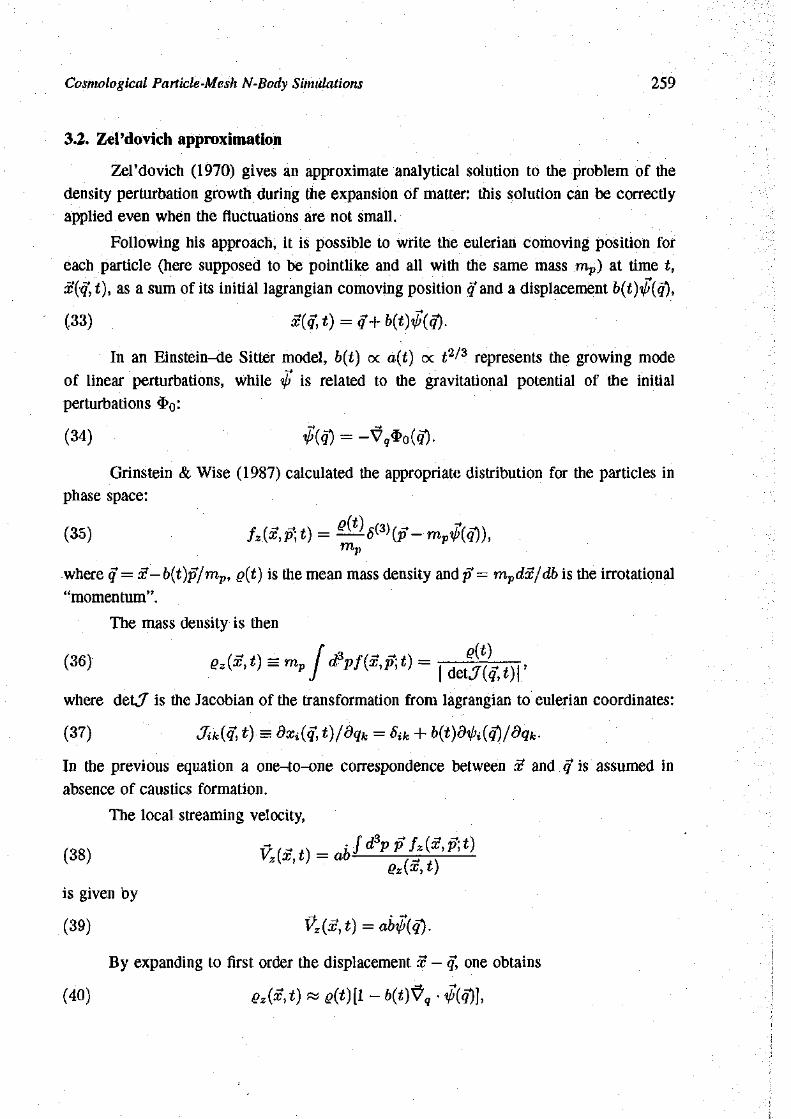
3.2. Zel'dovìch approximation

Zel'dovich (1970) gives an approximate analytical solution to the problem of the density perturbation growth during the expansion of matter: this solution can be correctly applied even when the fluctuations are not small.

Following his approach, it is possible to write the eulerian comoving position for each particle (here supposed to be pointlike and ali with the same mass rap) at time t, x{q,t), as a sum of its initial lagrangian comoving position <f and a displacement b(t)ip{q),

(33) mt) = <ì+b{t)${<i).

In an Einstein-de Sitter model, b(t) oc a(t) oc £2/3 represents the growing mode —•

of linear perturbations, while i/> is related to the gravitational potential of the initial perturbations 3>0:

(34) $(q) = -Vq$o(q).

Grinstein & Wise (1987) calculated the appropriate distribution for the particles in phase space:

(35) W^t) = —^){p-rnAq))ì

where q = x — b(t)p/mp, g(t) is the mean mass density andp*= mpdx/db is the irrotational "momentum".

The mass density is then

(36) Qz(x,t)=mp I\ d?pf{x,p\t) | d e t j ( £* ) r

where detj ' is the Jacobian of the transformation from lagrangian to eulerian coordinates:

(3.7) 'Jiktàt)-=dxi(q,t)/dqk = 6ik+-b(i)d$i(q)/dqk.

In the previous equation a one-to-one correspondence between x and q is assumed in absence of caustics formation.

The locai streaming velocity,

(38) Vz(x,t) = ab+ QZ\X,Z)

is given by

(39) Vz(x,t) = abif(^).

By expanding to first order the displacement x - q, one obtains

(40) Qz(x*,t)Ke{t)[l-b{t)Vq.${q)l

260 L. Moscardini

while the velocity field is easily obtained by substituting x with q in Eq.(39).

The primordial density fluctuations field 6 M O M ) gives $o by means of the Poisson equation A^3^o(x) = 6M(x,t)/b(t); therefore, in this way the particles give, without any limitation on the choice of the probability distribution, a faithful representation of the initial mass distribution and a peculiar velocity field satisfying the continuity equation. The validity of the method is however limited to the linear regime, i.e. 6 < 1.

3.3. Non-Gaussian case

The way to set non-Gaussian initial conditions for a iV-body code is more complicate: unlike the Gaussian case where ali characteristics of the distribution are described only by the power spectrum (or the two-point correlation function), in this case it is necessary to specify contemporarily the assumed distribution and the correlation functions-at ali orders. In this section we describe the method to construct initial conditions only for a small subset of non-Gaussian distributions: in particular we consider the same models described in Moscardini et al. (1991), Matarrese et al. (1991) and Messina et al. (1992).

The fundamental quantity is assumed to be the gravitational potential fluctuation field $, which is the typical gauge-invariant (up to a zero-mode) variable whose statistics is fixed by primordial processes, like in inflation. Ali our distributions are built up in such a way that $ has a power-spectrum

(41) , P#(*) = ^7>ok-3T\k),

where Vok is the primordial Zel'dovich spectrum of density fluctuations. We take the cold dark matter (CDM) transfer function (see, e.g., Davis et al. 1985)

(42) T{k) = [1 + l.lkl + 9.0(fc/)3/2 + l.O(W)2]"1,

with l = (tloh2)'1 Mpc; we consider only models with Q0 = 1.

The models we consider are obtained by the following procedure: the gravitational potential is taken as the convolution of a real function r{x) with a stationary, zero-mean, random field (p(x):

(43) *(à?) = Jd3yr(y-xMy).

The field cp will be related to one or more Gaussian random processes via some non-linear operation and the function r will be fixed by its Fourier transform,

(44) r(k) = / d3xe~i%-sr{x) = T(k) F(k),

where T(k) is the transfer function and F(k) is a positive correction factor, applied in order to obtain the exact CDM power spectrum in our finite simulati on box.

Cosmological Particle-Mesh N-Body Simulations 261

w\

Let us now describe in more details the application to some distributions.

i) Convolution

This is a model where the random field cp is given by the convolution

(45) tp(x) = d?y a(y - x)n(y)

where a is a real function, n and w are two independent zero-mean Gaussian flelds whose power spectra are

(46) Vn(k) = l,

so that n is white-noise [i.e. (n(x)n(y)) = 6^3\x-y)], and

27T2/C~3

(47) w = M w y *»^*<*M, with Vw(k) = 0 outside this A; interval. With such a choice w has unit variance (it/2) = 1. The white-noise character of n together with the w normalization implies that the y? auto-correlation function is completely determined by a, independently of the spectrum of w. Requiring that $ has a CDM spectrum implies that à(k) = (3/2)VQ/2k~3^2. This is essentially the same model proposed by Peebles (1983) and analysed in some detail by Lucchin & Matarrese (1988). They defined it directly for the density fluctuation; the two definitions are however equivalent at the linear level. The model turns out to be symmetric against the change $ —> — $', so that ali odd-order correlation functions vanish.

ii) Lognormal

A second type of models can be obtained by using the lognormal statistics for ip,

(48) <p(x)=A[ewW-(ew)],

where w is a zero-mean Gaussian field with unit variance and power spectrum as in Eq.(47). There is stili the freedom of assuming A to be negative (LNP model) or positive (LNn

model). The <p spectrum is then approximately given by

( 4 9 ) ^"^i»- : while the gravitational potential $ has the cold dark matter power spectrum with amplitude Po « 87T2eA2/9ln(kM/km). One would get different lognormal statistics according to the amplitude of w\ if (w2) were small the non-Gaussian character of tp would only manifest in rare high peaks; if, on the contrary, (w2) were large the ip power spectrum would deviate from flicker-noise. It is easy to calculate the three-point function of linear density fluctuations for this model; from it one finds that LNP (LNn) has positive (negative) skewness (hence the names we assigned to mese models). This model has been analysed

262 L. Moscardini

in a cosmological context by many authors (see e.g., Coles & Jones 1991 and references therein).

iii) Chi-squared

A third kind of distributions is obtained by considering a Chi-squared statistics with one degree of freedom:

(50) (p(x) = A[w2(x) - (w2)],

w being a Gaussian fluctuation field with the same power spectrum of Eq.(47). It can be shown that the <£> power spectrum is given by

2TT2A2

(51) V^k) « , 2n „ k-3[(3(k) + 21n(l + k/km) - l ] , In {kM/km)

where p(k) = (1 - k/km)2, for km < k < 2km, and (3{k) = 1 + 21n(-l + k/km), for 2km < k « kM. The Constant A can be either negative (xl model) or positive (xi model). The names are chosen according to the sign of (S^f), as before. For intermediate scales, the <E> power spectrum is dose to the standard CDM one with amplitude Vo « 2(47rA/3)2 \n(k/km)/\n2(kM/km). Chi-squared models have been considered by Coles & Barrow (1987), in connection with the two-dimensional statistics of CBR fluctuations. In the inflationary context, Salopek, Bond & Bardeen (1989) proposed a model where adiabatic perturbations are described by a squared Gaussian process, our x̂ > whose w field has a non-scale-free power spectrum.

To get the initial conditions for our simuiations, we first generate, by standard procedures (see Section 3.1), Gaussian realizations in momentum space with the required power spectrum: Eqs.(46) and (47) for C and Eq.(47) for LN and x2 models. The described non-linear transformations are applied in configuration space to get the non-Gaussian cp distributions. The actual gravitational potential $, to be processed by the Zel'dovich algorithm, is obtained by further Fourier transforming which allows a straightforward convolution of ip with the transfer function (the C model requires further convolution with the function a).

Before concluding this section let us make some general comments. First of ali it should be stressed that, in the general non-Gaussian case, a statistical distribution for $(£) does not imply the same distribution for 6M{X). Moreover, not any statistical distribution can be self-consistently assumed for 6M'- for instance, a Chi-squared distribution for 6M would imply a positive definite two-point function, which is in contrast with large-scale homogeneity, while the same statistics for $ does not lead to inconsistencies. The àssumption implicit in Eqs.(43) and (44) is that the statistics of $(Jb) is of primordial origin, i.e. it refers to the Urne when that fluctuation mode was outside the Hubble radius.

Cosmological Particle-Mesh N-Body Simulations 263

Also, the overall sign, which is just a phase, should be fixed by the primordial physical mechanism giving rise to the perturbation field. This statistics is left invariant in the linear regime independently of the physical processes which modify the fc-content of 3>, on every scale not involved by acoustic oscillations. It is worth to notice that the flicker-noise choice for the w spectrum, which gives equipartition in Fourier space, is stable (up to small corrections) against the non-linear operation leading to tp, both in x2 and LN models.

Both C and x2 models represent examples of scale-invariant non-Gaussian statistics (Otto et al. 1986; Lucchin & Matarrese 1988). On the other hand, x2 and LN statistics belong to the same general class (p(x) oc |1 + a~1w(x)\a\ in fact, for a. = 2 and {w2}1/2 » 1, the x2 distribution is recovered, while a —> oo yields the lognormal one. For small wave numbers, where T{k) « 1, the gravitational potential of scale-invariant distributions obeys the scaling law:

(52) (Ì>(/x£i) • -.$(p,kN))d3(fik1) • -d3(nkN) « (l>(£i) • • .$(£w))d3fci • • -d3kNì

for any N, up to logarithmic corrections owing to the cutoff wave numbers. This gives a straightforward generalization of the Harrison-Peebles-Zerdovich scale-invariance to non-Gaussian statistics. As a consequence, the particle distribution derived from the Zel'dovich algorithm, before shell-crossing, obeys a simple rule: the spatial distribution at Urne £2 will appear the same as it was at time ti provided that ali lengths are rescaled by the factor / * = ( * 2 / * i ) 1 / 3 .

3.4. Some results

Here we shortly discuss the results of a set of Ar-body simulations with non-Gaussian initial conditions and we compare them with the correspondihg results for simulations with Gaussian initial conditions. More details can be found in Moscardini et al. (1991), Matarrese et al. (1991), Messina et al. (1992) and Coles et al. (1993).

Our simulations represent the universe on a cube of 260 hrl Mpc side (h, the Hubble Constant in units of 100 km s_ 1 Mpc -1, was fixed to 0.5). Calculations were performed on a CRAY-YMP432 at the CINECA Computer Center in Bologna. A particle-mesh (PM) code was used with Np = 1283 particles on N9 = 1283 grid points. Each particle, representing a fluid element of dark matter, carries a mass of 4.7 x IO12 M©. We run two realizations for, each of the considered models. Periodic boundary conditions were adopted as usuai. We then performed a detailed statistical analysis of the present texture of our models using some relevant tests.

The main result of our analysis is that the primordial skewness of the mass fluctuations is a strongly discriminating parameter. The Convolution model, which is unskewed because it has vanishing odd-order correlation functions, presents only very modest differences when compared to the standard Gaussian model, while the Chi-squared

264 L. Moscardini

and the Lognormal statistics, characterized by an absolute value of the skewness parameter of order unity, show relevant changes. The non-linear evolution breaks the initial symmetry between positive and negative models, but the models with the same skewness sign show the same behavior in most statistical tests. Main properties of these distributions can be summarized as follows.

Skew-positive models appear lumpy on ali scales with isolated rich clusters emerging from a nearly uniform density fìeld. The analysis of the two-dimensional topology of mock catalogs drawn from our simulations (Coles et al. 1993) also revealed discrepancies with the properties of the Lick data. These conclusions agree with previous results (Moscardini et al. 1991; Weinberg & Cole 1992) and altogether seem to outline difficulties for the texture-seeded CDM model (see e.g. Park, Spergel & Turok 1991; Cen et al. 1991) which is very similar to this kind of models.

On the contrary, the structures in skew-negative models are characterized by a high level of connectivity with large voids surrounded by extended sheets and fìlaments. The clustering properties, as shown for example by galaxy correlation functions (Messina et al. 1992) and cluster multifractal analysis (Borgani et al. 1993), are in rather good agreement with observations, in particular for the xìi model. Weinberg & Cole (1992) recently evolved scale-free skew-negative models. They concluded that these models present many attractive properties, but fail in reproducing the cluster mass-to-light ratios, the pairwise velocities of galaxies and the expected type of topology. A partial explanation of these difficulties could be ascribed to the normalization they used to single out the present epoch from scale-free initial distributions.

In conclusion, phase correlations in the primordial perturbation fìeld play a relevant role in the non-linear evolution of cosmic structures. This kind of initial conditions may be motivated by physical models in the frame of the dynamics of phase transitions in the early universe. The present work has shown that a substantial predominance of primordial underdense regions (negative skewness) is a possible solution to the large-scale problem of the standard CDM scenario. Preserving the bottom-up hierarchical process, negative models succeed in producing a cellular structure with large correlation length and high bulk motions by the slow non-linear process of void merging and disruption of low-density shells.

Acknowledgments

We are grateful to Francesco Lucchin, Sabino Matarrese and Antonio Messina with whom much of the work reviewed here has been done and to Bepi Tormen for criticai reading of the manuscript.

Cosmological Particle-Mesh N-Body Simulations 265

REFERENCES

[1] AARSETH, S.J. 1971, Ap. Space Sci., 14, 118.

[2] BARDEEN, J.M., B O N D , J.R., KAISER, N., & SZALAY, S. 1986, ApJ, 304, 15.

[3] BORGANI, S., COLES, P . , MOSCARDINI, L., & PLIONIS, M. 1993, The angular momentum distribution ofclusters in skewed CDM models, MNRAS, in press.

[4] CEN, R., OSTRIKER, J .P . , SPERGEL, D.N., & T U R O K , N. 1991, ApJ, 383, 1.

[5] COLES, P . , & BARROW, J .D. 1987, MNRAS, 228, 407.

[6] COLES, P . , & JONES, B . J .T . 1991, MNRAS, 248, 1.

[7] COLES, P . , MOSCARDINI, L., PLIONIS, M., LUCCHIN, F., MATARRESE, S., MESSINA,

A. 1993, MNRAS, 260, 572.

[8] DAVIS, M., EFSTATHIOU, G., FRENK, C.S., & W H I T E , S.D.M. 1985, ApJ, 292, 371.

[9] EFSTATHIOU, G., DAVIS, M., FRENK, C.S., & W H I T E , S.D.M. 1985, ApJSS, 57, 241.

[10] GELB, J .M. 1992, Ph.D. Thesis, M.I.T.

[11] GRINSTEIN, B., & W I S E , M.B. 1987, ApJ, 316, 489.

[12] HOCKNEY, R.W., & EASTWOOD, J .W. 1981, Computer Simulations using Particles, McGraw-Hill, New York.

[13] LUCCHIN, F. , & MATARRESE, S. 1988, ApJ, 330, 535.

[14] MATARRESE, S., LUCCHIN, F. , MESSINA, A., & MOSCARDINI, L. 1991, MNRAS, 252, 35.

[15] MELOTT, A L . 1986, Phys. Rev. Lett, 56, 1992.

[16] MESSINA, A., LUCCHIN, F. , MATARRESE, S., & MOSCARDINI, L. 1992, Astroparticle Phys., 1, 99.

[17] MOSCARDINI, L., MATARRESE, S., LUCCHIN, F. , & MESSINA, A. 1991, MNRAS, 248,

424.

[18] O T T O , S., POLITZER, H.D., PRESKILL, J., & W I S E , M.B. 1986, ApJ, 304, 62.

[19] PARK, C , SPERGEL, D.N., & TUROK, N. 1991, ApJ, 372, L53.

[20] PEEBLES, P . J .E. 1980, The Large Scale Structure ofthe Universe, Princeton University Press, Princeton.

[21] PEEBLES, P . J .E . 1983, ApJ, 274, 1.

[22] SALOPEK, D.S., BOND, J.R., & BARDEEN, J.M. 1989, Phys. Rev., D40, 1753.

[23] W E I N B E R G , D.H., & C O L E , S. 1992, MNRAS, 259, 652.

[24] ZEL'DOVICH, Y A . B . 1970, A&A, 5, 84.

Lauro MOSCARDINI

Dipartimento di Astronomia, Università di Padova, vicolo dell'Osservatorio 5, 35122 Padova, Italy.

Lavoro pervenuto in redazione il 30.10.1993,