Krylov Subspace Methods for Simultaneous

Primal-Dual Solutions and Superconvergent

Functional Estimates

by

James Lu

Submitted to the Department of Aeronautics and Astronautics

in partial fulfillment of the requirements for the degree of

Master of Science in Aeronautics and Astronautics

at the

MASSACHUSETTS INSTITUTE OF TECHNOLOGY

Sept 2002

c© James Lu, MMII. All rights reserved.

The author hereby grants to MIT permission to reproduce anddistribute publicly paper and electronic copies of this thesis document

in whole or in part.

Author . . . . . . . . . . . . . . . . . . . . . . . . . . . . . . . . . . . . . . . . . . . . . . . . . . . . . . . . . . . . . .

Department of Aeronautics and AstronauticsAugust 23, 2002

Certified by. . . . . . . . . . . . . . . . . . . . . . . . . . . . . . . . . . . . . . . . . . . . . . . . . . . . . . . . . .

David L. DarmofalAssociate Professor

Thesis Supervisor

Accepted by . . . . . . . . . . . . . . . . . . . . . . . . . . . . . . . . . . . . . . . . . . . . . . . . . . . . . . . . .

Edward M. GreitzerProfessor of Aeronautics and Astronautics

Chair, Committee on Graduate Students

2

Krylov Subspace Methods for Simultaneous Primal-Dual

Solutions and Superconvergent Functional Estimates

by

James Lu

Submitted to the Department of Aeronautics and Astronauticson August 23, 2002, in partial fulfillment of the

requirements for the degree ofMaster of Science in Aeronautics and Astronautics

Abstract

This thesis is concerned with the iterative solution of non-symmetric linear (primal)systems and the dual systems associated with functional outputs of interest. Themain goal of the work is to arrive at efficient Krylov subspace implementations for thesituation where both primal and dual solutions are needed and accurate predictionsfor the functional outputs are desired.

A functional-output convergence result in the context of Krylov subspace methodsis given. It is shown that with an appropriate choice of the starting shadow vector,methods based on the nonsymmetric Lanczos process obtain iterates giving super-convergent functional estimates. Furthermore, the adjoint solution may be obtainedsimultaneously with essentially no extra computational cost. The proposed method-ology is demonstrated by the construction of a modified superconvergent variant ofthe QMR method.

The class of Krylov subspace methods based on Arnoldi process is also examined.Although by itself, superconvergence is not naturally present in the Arnoldi process,primal and dual problems may be coupled in a manner that allows for superconver-gence. In particular, the proposed methodology is demonstrated by the constructionof a primal-dual coupled superconvergent variant of the GMRES method.

Numerical experiments support the claim of superconvergence and demonstratethe viability of the proposed approaches.

Thesis Supervisor: David L. DarmofalTitle: Associate Professor

3

4

Acknowledgments

I would like to acknowledge the guidance and support of my thesis advisor, Professor

David Darmofal, who provided many insightful ideas and suggestions for the work

presented in this thesis. Thanks also goes to David Venditti for his assistance in

providing the FUN2D test case.

5

6

Contents

1 Introduction 11

2 Functional-output Convergence Results 15

2.1 Krylov Subspace Methods . . . . . . . . . . . . . . . . . . . . . . . . 15

2.1.1 Subspace Correction Framework . . . . . . . . . . . . . . . . . 15

2.1.2 Methods Based on Arnoldi Process . . . . . . . . . . . . . . . 16

2.1.3 Methods Based on Lanczos Process . . . . . . . . . . . . . . . 17

2.2 Adjoint Analysis . . . . . . . . . . . . . . . . . . . . . . . . . . . . . 17

2.2.1 Krylov Subspace Output Convergence Results . . . . . . . . . 19

3 Simultaneous Primal-Dual Superconvergent QMR 25

3.1 Nonsymmetric Lanczos Process . . . . . . . . . . . . . . . . . . . . . 25

3.2 Conventional QMR . . . . . . . . . . . . . . . . . . . . . . . . . . . . 29

3.3 Modifications for Simultaneous Dual Solution . . . . . . . . . . . . . 30

3.4 Preconditioning and Superconvergence . . . . . . . . . . . . . . . . . 32

3.5 Algorithm Implementation . . . . . . . . . . . . . . . . . . . . . . . . 36

3.6 Numerical Experiments . . . . . . . . . . . . . . . . . . . . . . . . . . 40

3.6.1 Example 1 . . . . . . . . . . . . . . . . . . . . . . . . . . . . . 40

3.6.2 Example 2 . . . . . . . . . . . . . . . . . . . . . . . . . . . . . 41

4 Coupled Primal-Dual Superconvergent GMRES 45

4.1 Coupling Strategy for Superconvergence . . . . . . . . . . . . . . . . 46

4.2 Arnoldi Process and Equality Constraint . . . . . . . . . . . . . . . . 46

7

4.2.1 Algorithm Implementation . . . . . . . . . . . . . . . . . . . . 48

4.2.2 CSGMRES Algorithm . . . . . . . . . . . . . . . . . . . . . . 50

4.3 Numerical Experiments . . . . . . . . . . . . . . . . . . . . . . . . . . 52

4.3.1 Example 1 . . . . . . . . . . . . . . . . . . . . . . . . . . . . . 52

4.3.2 Example 2 . . . . . . . . . . . . . . . . . . . . . . . . . . . . . 53

5 Conclusions and Future Work 57

A SSQMR MATLAB code 59

B CSGMRES MATLAB code 65

8

List of Figures

3-1 Plots from SSQMR Example 1 : Poisson problem . . . . . . . . . . . 43

3-2 Plots from SSQMR Example 2 : Euler flow . . . . . . . . . . . . . . . 44

4-1 Plots from CSGMRES Example 1 : Poisson problem . . . . . . . . . 54

4-2 Plots from CSGMRES Example 2 : Euler flow . . . . . . . . . . . . . 55

9

10

Chapter 1

Introduction

The need for the solution of nonsymmetric linear systems arises in a large variety of

situations. Among those is an important class that arise from the numerical solution

of partial differential equations (PDEs) modelling physical problems. For PDEs that

result from engineering analysis and design optimization, the principal quantities of

interest are often functional-outputs of the solution. With appropriate linearization of

the governing equation and the functional output, one often encounters linear systems

for the primal variable x of the form :

Ax = b, (1.1)

and the principal quantity of interest is a linear functional of the form,

Jpr(x) = gTx. (1.2)

Associated with the functional output of interest, one can consider the adjoint vector

y which is the solution to

ATy = g, (1.3)

11

and the associated dual functional,

Jdu(y) = bTy. (1.4)

With the primal and dual functional defined as in (1.2) and (1.4), we have the fol-

lowing equivalence,

Jpr(A−1b) = Jdu(A−Tg). (1.5)

The adjoint solution has found a multitude of uses in engineering computational

simulations. For instance, the adjoint can be employed in design optimization to

efficiently calculate the gradients of the outputs with respect to the control factors

(Jameson [25], Reuther, Jameson and Alonso [34], Giles and Pierce [21], Elliot and

Peraire [12], Anderson and Venkatakrishnan [3]). Furthermore, the adjoint solution

can be used to estimate and control errors in functional outputs of computational

simulations (Becker and Rannacher [6], Peraire and Patera [32], Giles and Pierce

[33], Venditti and Darmofal [46, 47, 45]). Motivated by the numerous uses of the

adjoint solution, this thesis is concerned with the situation where solutions for both

the primal and dual problem are required.

The main contributions of this thesis are twofold. Firstly, the simultaneous iter-

ation of both the primal and dual problems is demonstrated to have the benefit of

superconvergence. Secondly, efficient implementations of coupled primal-dual solu-

tions are presented.

Chapter 2 presents the underlying theory of Krylov subspace methods and de-

velops the concept of superconvergent functional estimates in the context of itera-

tive solution of linear systems. In Chapter 3, the nonsymmetric Lanczos process is

presented where it is demonstrated that the dual solution may be simultaneously

obtained with little additional computational costs and superconvergence may be

brought out naturally; a modified superconvergent variant of the quasi-minimal resid-

12

ual method is presented. Finally, in Chapter 4, the Arnoldi process for constructing

orthogonal bases is combined with superconvergence ideas to construct a smoothly

converging primal-dual coupled superconvergent variant of the generalized minimal

residual method.

13

14

Chapter 2

Functional-output Convergence

Results

2.1 Krylov Subspace Methods

In Sect. 2.1.1 the general subspace correction framework is described. Several Krylov

subspace methods are shown to lie in this framework, allowing the functional-output

convergence for those methods to be analyzed in a unified way, given in Sect. 2.2.

2.1.1 Subspace Correction Framework

Consider a sequence of nested finite-dimensional correction and test subspaces,

0 = C0 ⊆ C1 ⊆ · · · ⊆ CN ,

0 = T0 ⊆ T1 ⊆ · · · ⊆ TN , (2.1)

with the dimensions indexed by the subscripts. A subspace correction iterative

method for the primal linear system (1.1) obtains iterates xn satisfying

15

xn = x0 + cn, cn ∈ Cn,

rprn (xn) ⊥ t, ∀t ∈ Tn, (2.2)

where x0 is the initial guess and

rprn (xn) ≡ b− Axn. (2.3)

Krylov subspace methods lie in the general framework of subspace correction, limited

mostly to cases Cn = Kn(rpr0 ,A), where

Kn(rpr0 ,A) ≡ spanrpr

0 ,Arpr0 , · · · ,An−1r

pr0 , (2.4)

with an exception to this rule being GMERR [49]. We now describe a few commonly

used Krylov subspace methods that fit well into the subspace correction framework.

2.1.2 Methods Based on Arnoldi Process

The Arnoldi process generates an orthonormal basis of Kn(rpr0 ,A) with the disad-

vantage of entailing linearly growing memory and computational costs per itera-

tion. Amongst Krylov subspace methods, the most reknown are the Full Orthogonal

Method (FOM) [36] and the more stable Generalized Minimal Residual Method (GM-

RES) [38]. Let us consider applying FOM and GMRES to the primal linear system

(1.1). Table 2.1 summarizes the well-known properties of FOM and GMRES [11] in

the framework of (2.2). We note that the GMRES selection of subspaces is equivalent

to minimizing the residual in the case when xn = x0 + cn, cn ∈ Kn(rpr0 ,A).

16

FOM GMRES

Cn Kn(rpr0 ,A) Kn(r

pr0 ,A)

Tn Kn(rpr0 ,A) AKn(r

pr0 ,A)

Table 2.1: Subspaces for FOM and GMRES

BiCG QMR

Cn Kn(rpr0 ,A) Kn(rpr

0 ,A)Tn Kn(w1,A

T ) Un(w1,Ωprn ,AT )

Table 2.2: Subspaces for BiCG and QMR

2.1.3 Methods Based on Lanczos Process

Krylov subspace methods based on the non-symmetric Lanczos process requires two

starting vectors. Applied to the primal linear system (1.1), this class of method is

started by taking rpr0 and an arbitrary initial shadow vector w1, the only require-

ment being wT1 r

pr0 6= 0. Biorthogonal bases for two Krylov subspaces are gener-

ated, although only one of which is explicitly used in constructing the iterates xn.

The best-known methods based on the Lanczos process are Biconjugate Gradients

(BiCG) [13] and more stable Quasi-Minimal Residual method (QMR) [18]. For the

primal linear system (1.1), Table 2.2 summarizes the corresponding subspaces. Note

that Un(w1,Ωprn ,AT ) ≡ range(Wn+1D

−1n+1(Ω

prn )−1Ln) is a n–dimensional subspace of

Kn+1(w1,AT ) and Wn+1,Dn+1,Ω

prn ,Ln are matrices in the notation of [19]. Many

transpose-free variants of BiCG and QMR have been constructed [16], some of which

will be discussed later.

2.2 Adjoint Analysis

For the iterative solution of the linear system (1.1), we have the following a priori

error norm estimate,

17

‖x − xn‖ ≤ ‖A−1‖‖rprn ‖. (2.5)

The above estimate is optimal in the sense that no higher exponent on the residual

norm is possible. Thus, in general the norm of the solution error and arbitrary output

functionals are expected to converge at a rate no higher than that of the residual.

Under the special circumstances that certain functionals of the approximate solution

converge at orders of the residual norm higher than that given by the global error

estimate (2.5), those quantities are said to be superconverging. In particular, an iter-

ative method is defined to be superconvergent if the superconvergence phenomenon

can be demonstrated for arbitrary linear systems and linear functionals. This usage of

the term superconvergence is a carry over of a concept usually used in contexts such

Galerkin finite element methods to describe the convergence of functional estimates

[1, 48]. Note that this phenomenon is distinct from superconvergence as used in [8]

to loosely describe the faster residual convergence when certain projected solutions

are used as initial guess. The question of whether an iterative procedure is super-

convergent may be settled using adjoint analysis. Denote y as an arbitrary adjoint

approximation and rdu the corresponding dual residual defined by

rdu = g − AT y. (2.6)

The error in the functional-output provided by a primal iterate xn may be written

as,

Jpr(x) − Jpr(xn) = yT rprn + (rdu)T (A−1rpr

n ). (2.7)

Using the triangle inequality and taking the infimum over all y, it follows that the

error in the functional output provided by the primal iterates is bounded by the

18

following :

|Jpr(x) − Jpr(xn)| ≤ miny

(

|yT rprn | +

‖rdu‖‖rprn ‖

σmin

)

, (2.8)

where σmin denotes the smallest singular value of A, satisfying

σmin = minz,z6=0

‖Az‖

‖z‖. (2.9)

As an immediate consequence, for general subspace correction methods (2.2),

|Jpr(x) − Jpr(xn)| ≤ miny∈Tn

‖rdu‖‖rprn ‖

σmin

. (2.10)

The above bound suggests that the convergence of functional estimates provided by

subspace correction methods is controlled by the residual norm of the primal iterates

as well as the closeness of approximation the sequence of test spaces for the primal

problem, Tn, provide for the adjoint solution.

2.2.1 Krylov Subspace Output Convergence Results

In this section, functional-output convergence results for the Krylov methods of

Sect. 2.1 and Sect. 2.2 are obtained by applying the bound (2.10).

FOM In the FOM approach, the bound (2.10) gives,

|Jpr(x) − Jpr(xprn )| ≤ min

y∈Kn(rpr0 ,A)

‖rdu‖‖rFOM,prn ‖

σmin. (2.11)

Thus, for FOM iterates the functional convergence rate can be determined by the

approximation of the dual problem over the nested subspaces Kn(rpr0 ,A) :

19

‖rdun ‖ ≡ min

y∈Kn(rpr0 ,A)

‖g − AT y‖. (2.12)

The above minimization problem is equivalent to the orthogonality condition,

rdun ⊥ ATKn(rpr

0 ,A). (2.13)

The fact that (2.13) implies (2.12) may be shown by the following argument. Denote

yn as the minimizer corresponding to the minimal residual of (2.12) and y to be an

arbitrary vector in Kn(rpr0 ,A). Then, we have

‖g − AT y‖2 = ‖g − AT [(y − yn) + yn]‖2

= ‖g − AT yn‖2 − 2(g − AT yn,AT (y − yn))

+ ‖AT (y − yn)‖2. (2.14)

By the orthogonality condition (2.13), the middle term of the above expression is

zero. Hence, yn is the minimizer :

‖g − AT y‖2 ≥ ‖g −AT yn‖2 ∀y ∈ Kn(r

pr0 ,A). (2.15)

(2.12) is equivalent to solving the dual problem within the framework of a family of

generalized minimum error (GMERR) methods as described by Weiss [49]. Specifi-

cally, a GMERR method applied to the dual system finds iterates yGMERRn within the

Krylov subspaces generated by A,

yGMERRn ∈ y0 + AKn(p0,A), (2.16)

20

where p0 is an arbitrary starting vector and yGMERRn is chosen so that the error norm

is minimized,

‖y − yGMERRn ‖ = min

y∈y0+AKn(p0,A)‖y − y‖. (2.17)

In a manner similar to (2.14), it may be shown that the minimization property (2.17)

is equivalent to the error orthogonality condition,

y − yGMERRn ⊥ AKn(p0,A), (2.18)

and hence to the residual orthogonality condition,

g −ATyGMERRn ⊥ Kn(p0,A). (2.19)

Therefore, with the identification p0 = AT rpr0 and y0 = 0, the approximation problem

(2.12) is the same as (2.17). The convergence of GMERR for arbitrary p0 has not

been shown. For the case that p0 = g, it is known that the subspaces Kn(p0,A)

form a sequence of convergent approximations for the adjoint solution if and only if

A is normal [10]. In fact, unless A is normal and rpr0 related to g in some way, the

convergence of (2.12) is expected to be poor. Hence, functional estimates obtained

from FOM iterates are expected to converge at a rate no higher than that of the

residual norm.

GMRES For GMRES, the functional error bound (2.10) is :

|Jpr(x) − Jpr(xGMRESn )| ≤ min

y∈AKn(rpr0 ,A)

‖rdu‖‖rGMRES,prn ‖

σmin. (2.20)

Analogous to the FOM case discussed above, for GMRES iterates the convergence

21

rate of functional estimates is controlled by :

‖rdun ‖ ≡ min

y∈AKn(rpr0 ,A)

‖g −AT y‖. (2.21)

In general, the above is not an improvement over (2.12). Hence, the conclusion is

also that the functional estimates obtained from GMRES iterates is only linearly

convergent with the residual norm.

BiCG For bi-conjugate gradients, the functional error bound is,

|Jpr(x) − Jpr(xBiCGn )| ≤ min

y∈Kn(w1,AT )

‖rdu‖‖rBiCG,prn ‖

σmin. (2.22)

If GMRES is applied to the dual problem (1.3) with the zero vector as the initial

guess, the dual residual norm is minimized,

‖rGMRES,dun ‖ = min

y∈Kn(g,AT )‖g − AT y‖. (2.23)

Hence, if the test space for BiCG is started with w1 = g, we have the following bound,

|Jpr(x) − Jpr(xBiCGn )| ≤

‖rGMRES,dun ‖‖rBiCG,pr

n ‖

σmin. (2.24)

If A is relatively well-behaved so that the eigenvalue convergence bound is descriptive,

‖rGMRES,dun ‖ converges to zero at a rate bounded by ‖rBiCG,pr

n ‖. This shows that

BiCG with w1 = g is superconvergent at double the residual convergence rate for the

functional (1.2). For other choices of test space starting vectors, for example w1 = rpr0

as is almost always used in implemenetations, superconvergence for Jpr does not hold.

Numerical evidence for this behavior is shown in a future paper [29].

22

QMR Finally, we examine the convergence bound for QMR,

|Jpr(x) − Jpr(xQMRn )| ≤ min

yn∈Un(w1,Ωprn ,AT )

‖rdun ‖‖rQMR,pr

n ‖

σmin

. (2.25)

Similar to the BiCG case, QMR is not superconvergent if the starting shadow vector

for the non-symmetric Lanczos process w1 6= g. Convergence of functional esti-

mates is expected to improve significantly if w1 = g, as can be seen in some of

the numerical examples presented in Chapter 3. Also in Chapter 3, a metric for

quasi-residual minimization is chosen with demonstrated improved output conver-

gence. Viewed in the framework introduced here, this is equivalent to modifying the

subspace Un(g,Ωprn ,AT ) through the choice of Ωpr

n .

23

24

Chapter 3

Simultaneous Primal-Dual

Superconvergent QMR

In this chapter, the QMR algorithm is discussed in detail with the view towards im-

plementation, building on the more abstract description given in the previous chapter.

Firstly, the underlying non-symmetric Lanczos process is presented, showing how the

left shadow vector w1 may be chosen arbitrarily. Then, it is shown that besides

the improved functional convergence as already demonstrated, choosing w1 = g has

the additional advantage that the dual solution may be obtained simultaneously and

at little extra cost using the same Lanczos process. Lastly, based on the adjoint

analysis already presented, an approach to further improve functional convergence is

developed.

3.1 Nonsymmetric Lanczos Process

The nonsymmetric Lanczos process constructs biorthogonal and A-orthogonal basis

vectors of Krylov subspaces which are then used in methods such as QMR. That is,

it constructs vectors vj ’s and wj ’s that satisfy the biorthogonality condition

25

wTmvn =

δn, m = n,

0, m 6= n.

(3.1)

and vectors pj and qj that satisfy the A-orthogonality condition

qTmApn =

ǫn, m = n,

0, m 6= n.

(3.2)

We use the Lanczos process based on coupled two-term recurrences rather than that

based on three-term recursions as used in [18] since even though they are mathemat-

ically equivalent, the former is numerically more robust than the latter, as observed

in [19]. Also, to simplfy matters the look-ahead process [17] is not included.

• Initialization

– Normalize initial vectors v1 and w1.

– Set p0 = q0 = 0, ǫ0 = ρ1 = ξ1 = 1, n = 1.

• At iteration n :

1. If ǫn−1 = 0, stop. Otherwise compute δn = wTnvn. If δn = 0, then stop.

2. Update

pn = vn − pn−1(ξnδn/ǫn−1),

qn = wn − qn−1(ρnδn/ǫn−1) (3.3)

3. Compute

26

ǫn = qTnApn,

βn = ǫn/δn. (3.4)

Update

vn+1 = Apn − vnβn, ρn+1 = ‖vn+1‖,

wn+1 = ATqn −wnβn, ξn+1 = ‖wn+1‖. (3.5)

4. If ρn+1 = 0 or ξn+1 = 0, then stop. Else, update

vn+1 = vn+1/ρn+1,

wn+1 = wn+1/ξn+1. (3.6)

The result of the above iteration may be summarized compactly. Firstly, we introduce

the notation

Vn ≡

[

v1 v2 · · · vn

]

,

Wn ≡

[

w1 w2 · · · wn

]

,

Pn ≡

[

p1 p2 · · · pn

]

,

Qn ≡

[

q1 q2 · · · qn

]

. (3.7)

Then, it may be seen from the Lanczos process that the above satisfies

Vn = PnUn,

27

Wn = QnΓ−1n UnΓn,

APn = Vn+1Ln,

ATQn = Wn+1Γ−1n+1LnΓn, (3.8)

where the matrices Γn, Un and Ln are defined as

Γn = diag(γ1, γ2, · · · , γn), (3.9)

Un =

1 ξ2δ2/ǫ1 0 · · · 0

0 1 ξ3δ3/ǫ2 · · · 0

0 0 1 · · · 0

0. . .

. . .. . . ξnδn/ǫn−1

0 · · · · · · 0 1

, (3.10)

Ln =

β1 0 0 · · · 0

ρ2 β2 0 · · · 0

0 ρ3 β3 · · · 0

0 0 ρ4 · · · 0

0. . .

. . .. . . βn

0 · · · · · · 0 ρn+1

, (3.11)

the scalars ξj, δj, ǫj , ρj are constants defined in the Lanczos process, and the constants

γj satisfy the relation

γj =

1 j = 1,

γj−1ρj/ξj 1 < j ≤ n.

(3.12)

28

In the next section, we give a brief description of how QMR uses the Lanczos process

to generate iterates that approximate the linear system (1.1).

3.2 Conventional QMR

At each iteration, QMR seeks an iterate xprn within the Krylov subspace

xn ∈ x0 + spanrpr0 ,Ar

pr0 ,A2r

pr0 , · · · ,An−1r

pr0 . (3.13)

With the initial vector taken to be the normalized initial residual, v1 ≡ rpr0 /ρ1,

ρ1 ≡ ‖rpr0 ‖, it may be seen from the Lanczos process that

spanv1,v2, · · · ,vn = spanrpr0 ,Ar

pr0 ,A2r

pr0 , · · · ,An−1r

pr0 . (3.14)

Hence, from (3.13) xprn may be written as

xn = x0 + VnU−1n zn, (3.15)

where the matrices Vn, Un are defined in (3.7) and (3.10) respectively and the vector

zn is yet to be determined. Using the identities given in (3.8), it may be seen that

rprn = b− Axn

= rpr0 −Vn+1Lnzn. (3.16)

Using the fact that v1 = rpr0 /ρ1, and introducing an (n+1)× (n+1) diagonal weight

matrix Ωprn

29

Ωprn = diag(ωpr

1 , ωpr2 , · · · , ωpr

n+1), (3.17)

(3.16) may be written as

rprn = Vn+1

(

Ωprn

)−1(

ρ1ωpr1 en+1

1 − Ωprn Lnzn

)

. (3.18)

Finally, zn is chosen so that the 2-norm of the quasi-residual is minimized :

zn = argminz

∥

∥

∥

∥

ρ1ωpr1 en+1

1 −Ωprn Lnz

∥

∥

∥

∥

. (3.19)

Since the matrix Ln has a bidiagonal structure, the above minimization may be done

recursively, essentially performing QR decomposition of Ln using successive Givens

rotations.

The original QMR algorithm is formulated with a diagonal weighting matrix Ωn

and convergence has been shown for arbitrary weights ωprj 6= 0 [18]. Extension of the

weight matrix to block diagonal form having upper triangular blocks has also been

done [41]. However, in practice the weight matrix is usually set to unity owing to

the lack of a better choice. Moreover, in practice the two starting vectors are usually

taken to be the same and the fact that the same Lanczos iteration contains a dual

problem is not utilized. The desire of not using AT partly led to the development of

transpose-free variants of QMR [14, 20].

3.3 Modifications for Simultaneous Dual Solution

With modifications to the conventional QMR algorithm, the solution of the dual prob-

lem may be found simultaneously with the primal problem using the same Lanczos

process. Firstly, we observe that (3.8) implies not only

30

AVn = Vn+1LnUn, (3.20)

but also

ATWn = Wn+1Γ−1n+1LnUnΓn. (3.21)

This suggests taking the normalized shadow starting vector w1 for the Lanczos process

to be

w1 =g

ξ1, ξ1 = ‖g‖. (3.22)

It may be observed that in the Lanczos process, given a certain v1, the choice of

w1 is arbitrary so long as wT1 v1 6= 0. Only in rare circumstances will the non-

orthogonality condition not be satisfied. Note that this is a departure from the

standard implementation of QMR, which chooses the starting vector for the Lanczos

iteration to be w1 = v1.

Similar to the primal iterates, we seek iterates for the dual problem of the form

yn = WnΓ−1n U−1

n Γnkn, (3.23)

where the vector kn is yet to be determined. Then, the dual residual rdun is of the

form

rdun = g − ATyn

31

= Wn+1

(

Ωdun

)−1(

ξ1ωdu1 en+1

1 −Ωdun Γ−1

n+1LnΓnkn

)

, (3.24)

where the dual weight parameter matrix Ωdun has been introduced. Analogous to

the approach of QMR for the primal problem, kn is sought to minimize the 2-norm

quasi-residual :

kn = argmink

∥

∥

∥

∥

ξ1ωdu1 en+1

1 − Ωdun Γ−1

n+1LnΓnk

∥

∥

∥

∥

. (3.25)

Note that the term Γ−1n+1LnΓn in (3.24) is the analog of Ln in (3.16). In fact,

Γ−1n+1LnΓn =

β1 0 · · · 0

ξ2 β2 · · · 0

0. . .

. . . 0

0. . . ξn βn

0 · · · 0 ξn+1

, (3.26)

and comparison with Ln defined in (3.11) shows that Γ−1n+1LnΓn is just Ln with the

replacement ρj → ξj. Thus, the adjoint iterates yn may be obtained from the Lanczos

vectors with the same procedure as the standard QMR method for the primal problem

by replacing vj → wj , pj → qj and ρj → ξj.

3.4 Preconditioning and Superconvergence

For Krylov subspace methods, preconditioning is often necessary for fast and robust

convergence. In this section, a superconvergence strategy for the preconditioned sys-

tem is presented. It is shown that same strategy may be applied to both the primal

and the dual system.

With the use of preconditioners M1 and M2, the primal problem (1.1) effectively

becomes

32

A′x′ = b′, where A′ ≡ M−11 AM−1

2 ,

x′ ≡ M2x,

b′ ≡ M−11 b. (3.27)

The value of the primal linear functional is required to be invariant under the pre-

conditioning transformation, that is,

Jpr(x) = gTx=g′Tx′, (3.28)

thereby obtaining the expression for g′,

g′ = M−T2 g. (3.29)

Then, the adjoint for the preconditioned system, y′, is just the solution to

A′Ty′ = g′. (3.30)

From (3.30), it may be verified that

y′ = MT1 y. (3.31)

Furthermore, from (3.30) and (3.27),

bTy = b′Ty′. (3.32)

33

Equation (3.31) shows that the adjoint for the original system (1.3) may be recovered

from that of the preconditioned system by simply multiplying with the matrix M−T1

at the end of the iterations. In what follows, we will work exclusively with the

preconditioned systems.

As a means of improving the output superconvergence, we seek to minimize

(y′n+1)

T r′n (3.33)

where y′n+1 is an estimate of the adjoint available at the (n + 1)th iteration and r′n

is the primal residual at the nth iteration, both for the preconditioned system. Note

that the check mark on y′n+1 is used to differentiate the adjoint estimates that we

use to determine weight parameters and the adjoint estimates carried forward in our

simultaneous primal-dual method.

The above provides a natural scaling for the QMR weight parameters. Specifically,

by letting,

ωprj = (y′

n+1)Tvj, 1 ≤ j ≤ n + 1, (3.34)

then,

(y′n+1)

T r′prn = (y′

n+1)T

[

v1 v2 · · · vn+1

](

Ωprn

)−1(

ρ1ωpr1 e

(n+1)1 − Ωpr

n Lnzn

)

=

[

(y′n+1)

Tv1 · · · (y′n+1)

Tvn+1

](

Ωprn

)−1(

ρ1ωpr1 e

(n+1)1 − Ωpr

n Lnzn

)

=[

1 1 · · · 1]

(

ρ1ωpr1 e

(n+1)1 − Ωpr

n Lnzn

)

. (3.35)

Thus, with the ωprj as chosen in (3.34), the linear error term (3.33) in the linear

functional is approximately equal to the sum of the entries of the primal quasi-residual.

By selecting zn to minimize this weighted primal quasi-residual, the primal iterates

34

obtained from our modified QMR approach should more accurately approximate the

linear functional.

However, the scheme as described above could suffer from non-recursivity because

at each iteration n, all weights ωprj , 1 ≤ j ≤ n must be updated and all prior vectors

might need to be stored. To maintain recursivity, we introduce a truncated approxi-

mation to the adjoint, y′i,n+1, where the index i is an approximation parameter. We

define y′i,n+1 as

y′i,n+1 ≡

(

(Y′i+1)

Tv1

wT1 v1

)

w1 +

(

(Y′i+2)

Tv2

wT2 v2

)

w2 + · · ·+

(

(Y′i+n+1)

Tvn+1

wTn+1vn+1

)

wn+1,

(3.36)

where we take Y′i to be the adjoint iterate from the standard QMR algorithm. Al-

though other choices may be thought of, using this truncated approximation, we

have

(y′i,n+1)

Tvj = (Y′i+j)

Tvj . (3.37)

Associated with a certain choice of i is the storage needed for the i vectors [p1 · · · pi],

each of the dimension of problem size. However, no extra computational work is

required. For the numerical experiments considered here, a small i (≈ 3) works well

enough.

With y′i,n+1 as defined in (3.37), we take the weight parameters to be

ωprj = (y′

i,n+1)Tvj

= (Y′i+j)

Tvj . (3.38)

A similar strategy of weight parameter determination may be done for the dual prob-

lem. Analogous to (3.38), we take the dual weights to be

35

ωduj = (X′

i+j)Twj , (3.39)

where similarly, X′n is the primal solution estimate obtained at iteration n using the

QMR method.

It is to be noted that although (3.38) and (3.39) imply forming the QMR iterates

X′n and Y′

n and performing inner products for the calculation of each weight, this

is not necessary. Instead, they are equivalently but cheaply calculated from scalars

obtained in the i Lanczos iterations ahead of the current primal and dual iterates.

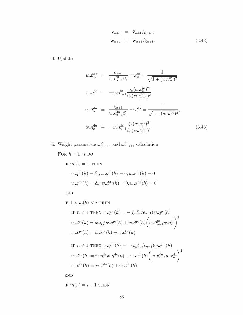
3.5 Algorithm Implementation

In this section, an implementation of the superconvergent simultaneous primal-dual

QMR (SSQMR) method is described. The Lanczos iteration is carried i steps ahead

of both the primal and dual iterates. Compared to conventional QMR, it requires a

constant extra storage of two sets of vectors P = [p1 p2 · · · pi] and Q = [q1 q2 · · · qi]

where each vector is of the same size as b. Additionally, three sets of i scalars need

to be stored : β = [β1 β2 · · · βi], ρ = [ρ1 ρ2 · · · ρi] and ξ = [ξ1 ξ2 · · · ξi]. After

convergence by some criteria, the primal and dual solutions for the original systems

are recovered by observing (3.27) and (3.31). The algorithm for SSQMR is given

below; MATLAB code is given in Appendix A.

Algorithm with Lanczos Forward Index i :

• Initialization

– Set initial guesses to be the zero vector : xpr0 = xdu

0 = 0.

– Let ρ1 = ‖M−11 b‖, v1 = M−1

1 b/ρ1. Let ξ1 = ‖M−T2 g‖, w1 = M−T

2 g/ξ1.

– Check that wT1 v1 6= 0, otherwise restart.

– Set p0 = q0 = dpr0 = ddu

0 = 0.

36

– Set cpr0 = cdu

0 = ǫ0 = 1, ϑpr0 = ϑdu

0 = 0, ηpr0 = ηdu

0 = −1.

– Set w cpr0 = w cdu

0 = 1, w ϑpr0 = w ϑdu

0 = 0, w ηpr0 = w ηdu

0 = −1.

– Initialize vector storage P = [p1 p2 · · · pi] and Q = [q1 q2 · · · qi], scalar

storage β = [β1 β2 · · · βi], ρ = [ρ1 ρ2 · · · ρi] and ξ = [ξ1 ξ2 · · · ξi].

– Set counter values for weight parameter accumulation :

k0 = 1

for h = 1 : i do

m(h) = 2 − h

end

• For n = 1, 2, 3, · · · , do

1. If ǫn = 0 or δn = 0, stop. Otherwise, compute δn = wTnvn.

2. Update counter kn = (kn mod i) + 1. Update vectors

pn = vn − pn−1(ξnδn/ǫn−1),

qn = wn − qn−1(ρnδn/ǫn−1). (3.40)

Store P(:, kn) = pn, Q(:, kn) = qn.

3. Compute pn = A(M−12 pn) and qn = M−T

1 qn. Update ǫn = qTn pn, and set

βn = ǫn/δn.

Update

vn+1 = M−11 pn − βnvn,

wn+1 = M−T2 (AT qn) − βnwn. (3.41)

Update ρn+1 = ‖vn+1‖, ξn+1 = ‖wn+1‖. Store β(kn) = βn, ρ(kn) = ρn,

ξ(kn) = ξn

If ρn+1 6= 0 and ξn+1 6= 0, update

37

vn+1 = vn+1/ρn+1,

wn+1 = wn+1/ξn+1. (3.42)

4. Update

w ϑprn =

ρn+1

w cprn−1βn

, w cprn =

1√

1 + (w ϑprn )2

,

w ηprn = −w ηpr

n−1

ρn(w cprn )2

βn(w cprn−1)

2

w ϑdun =

ξn+1

w cdun−1βn

, w cdun =

1√

1 + (w ϑdun )2

,

w ηdun = −w ηdu

n−1

ξn(w cdun )2

βn(w cdun−1)

2(3.43)

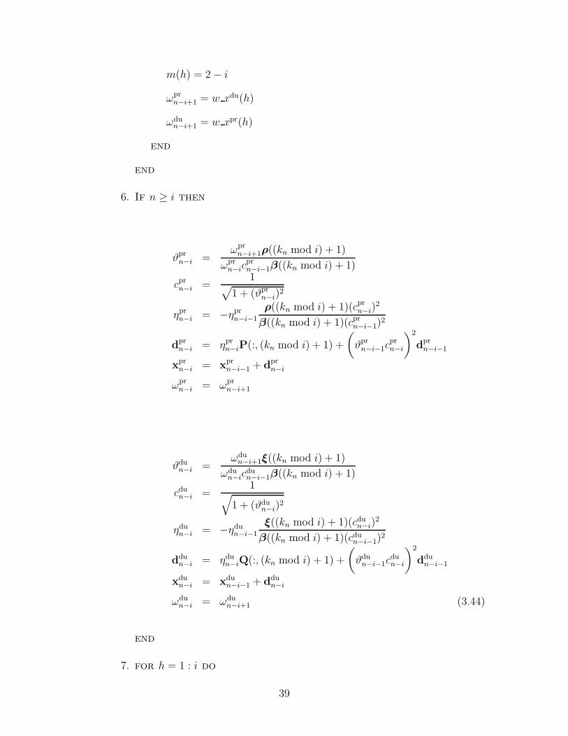
5. Weight parameters ωprn−i+1 and ωdu

n−i+1 calculation

For h = 1 : i do

if m(h) = 1 then

w qpr(h) = δn, w dpr(h) = 0, w xpr(h) = 0

w qdu(h) = δn, w ddu(h) = 0, w xdu(h) = 0

end

if 1 < m(h) < i then

if n 6= 1 then w qpr(h) = −(ξnδn/ǫn−1)w qpr(h)

w dpr(h) = w ηprn w qpr(h) + w dpr(h)

(

w ϑprn−1w cpr

n

)2

w xpr(h) = w xpr(h) + w dpr(h)

if n 6= 1 then w qdu(h) = −(ρnδn/ǫn−1)w qdu(h)

w ddu(h) = w ηdun w qdu(h) + w ddu(h)

(

w ϑdun−1w cdu

n

)2

w xdu(h) = w xdu(h) + w ddu(h)

end

if m(h) = i − 1 then

38

m(h) = 2 − i

ωprn−i+1 = w xdu(h)

ωdun−i+1 = w xpr(h)

end

end

6. If n ≥ i then

ϑprn−i =

ωprn−i+1ρ((kn mod i) + 1)

ωprn−ic

prn−i−1β((kn mod i) + 1)

cprn−i =

1√

1 + (ϑprn−i)

2

ηprn−i = −ηpr

n−i−1

ρ((kn mod i) + 1)(cprn−i)

2

β((kn mod i) + 1)(cprn−i−1)

2

dprn−i = ηpr

n−iP(:, (kn mod i) + 1) +

(

ϑprn−i−1c

prn−i

)2

dprn−i−1

xprn−i = x

prn−i−1 + d

prn−i

ωprn−i = ωpr

n−i+1

ϑdun−i =

ωdun−i+1ξ((kn mod i) + 1)

ωdun−ic

dun−i−1β((kn mod i) + 1)

cdun−i =

1√

1 + (ϑdun−i)

2

ηdun−i = −ηdu

n−i−1

ξ((kn mod i) + 1)(cdun−i)

2

β((kn mod i) + 1)(cdun−i−1)

2

ddun−i = ηdu

n−iQ(:, (kn mod i) + 1) +

(

ϑdun−i−1c

dun−i

)2

ddun−i−1

xdun−i = xdu

n−i−1 + ddun−i

ωdun−i = ωdu

n−i+1 (3.44)

end

7. for h = 1 : i do

39

m(h) = m(h) + 1

end

• Obtain primal and dual solutions for the original systems

Primal solution = (M2)−1xpr

n ,

Dual solution = (M1)−Txdu

n . (3.45)

3.6 Numerical Experiments

The proposed method with weight parameters determined using equations (3.38) and

(3.39) is denoted as Superconvergent Simultaneous QMR (SSQMR). The method

which solves both the primal and the dual problem but with all weight parameters set

to unity is denoted as Simultaneous QMR (SQMR). The conventional QMR method

has unity weights and initial vectors are chosen to be the same : w1 = v1. QMR is

separately applied to the primal and dual problems and the results are compared to

SSQMR and SQMR.

For all the examples shown here, the Lanczos forward index i for SSQMR is taken

to be 3, since this has been shown to give good results. Also, the initial guesses x′0

and y′0 for all the methods are chosen to be the zero vector. No convergence criteria is

used; rather, the number of iteration steps is specified in each case. The test problems

are not excessively large so that the solutions for the linear systems are available up

to level of round-off.

3.6.1 Example 1

In this example, we consider the second order finite difference discretization on a

51 × 51 grid of

∇2u =1

πexp−(x+2)2−(y−1/2)2 , Ω ∈ [0, 1] × [0, 1],

40

u|Γ = 0, (3.46)

resulting in the matrix A with 12205 non-zero elements. The linear functional is the

discretized approximation of

∫ 1

0

∫ 1

0

u(x, y) sin(πx) sin(πy)dxdy. (3.47)

The left and right preconditioners were obtained from the incomplete LU factorization

of A using a drop tolerance of 2×10−2, resulting in L and U having 12059 and 12057

non-zero elements respectively.

From Figure 3-1 it may be seen that the primal and dual functional estimates

obtained using standard QMR converge at roughly the same rate as the respective

residual norms, showing that it is not superconvergent. SQMR obtains better func-

tional estimates as a result of the better choice of starting vectors. In fact, the method

appears to exhibit superconvergence. However, the behavior is not very consistent.

On the other hand, SSQMR obtains functional estimates that are consistently super-

converging at twice the order of residual convergence and improvement in functional

estimates over SQMR is clearly seen.

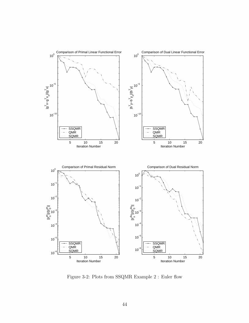
3.6.2 Example 2

In this example, the linear system considered is one arising from a first order back-

ward Euler implicit scheme for solving a first order upwind discretization of the two-

dimensional compressible flow Euler equations using the NASA Langley unstructured

flow solver FUN2D [2]. The specific problem is the transonic flow around the NACA

0012 airfoil (freestream Mach number of 0.8 and 1.25 degrees angle of attack). The

mesh is composed of 1980 triangular elements with 990 nodes. The linear output is

the airfoil drag functional linearized about the current iterate.

The matrix A has 108532 non-zero entries. The left and right preconditioners were

obtained from the incomplete LU factorization of A using a drop tolerance of 10−2,

41

resulting in L and U having 88253 and 93588 non-zero elements respectively. Again,

from Figure 3-2 we observe that the functional error convergence slopes of SSQMR are

roughly twice that of conventional QMR, confirming the prediction made regarding

superconvergence. In this example, the functional error of SQMR is close to that of

SSQMR, showing that the unity parameter happens to be quite a good choice in this

case. Still, SSQMR consistently gives better functional estimates than SQMR.

42

5 10 15 20

10−12

10−10

10−8

10−6

10−4

10−2

100

Iteration Number

|gTx−

gTx n|/|

gTx|

Comparison of Primal Linear Functional Error

SSQMRQMR SQMR

5 10 15 20

10−12

10−10

10−8

10−6

10−4

10−2

100

Iteration Number

|bTy−

bTy n|/|

bTy|

Comparison of Dual Linear Functional Error

SSQMRQMR SQMR

5 10 15 20

10−5

10−4

10−3

10−2

10−1

100

Iteration Number

||rnpr

||/||r

0pr||

Comparison of Primal Residual Norm

SSQMRQMR SQMR

5 10 15 20

10−6

10−5

10−4

10−3

10−2

10−1

100

Iteration Number

||rndu

||/||r

0du||

Comparison of Dual Residual Norm

SSQMRQMR SQMR

Figure 3-1: Plots from SSQMR Example 1 : Poisson problem

43

5 10 15 20

10−10

10−5

100

Iteration Number

|gTx−

gTx n|/|

gTx|

Comparison of Primal Linear Functional Error

SSQMRQMR SQMR

5 10 15 20

10−10

10−5

100

Iteration Number

|bTy−

bTy n|/|

bTy|

Comparison of Dual Linear Functional Error

SSQMRQMR SQMR

5 10 15 2010

−6

10−5

10−4

10−3

10−2

10−1

100

Iteration Number

||rnpr

||/||r

0pr||

Comparison of Primal Residual Norm

SSQMRQMR SQMR

5 10 15 20

10−6

10−5

10−4

10−3

10−2

10−1

100

Iteration Number

||rndu

||/||r

0du||

Comparison of Dual Residual Norm

SSQMRQMR SQMR

Figure 3-2: Plots from SSQMR Example 2 : Euler flow

44

Chapter 4

Coupled Primal-Dual

Superconvergent GMRES

GMRES [38] has found widespread use because of its robustness and its residual min-

imization property. However, as demonstrated in Chapter 2, it is not superconvergent

since the sequence of test spaces Tn do not approximate the adjoint well.

A way to make the adjoint Krylov subspace available is to iterate the dual problem

in parallel with the primal. However, taking the adjoint Krylov subspace as the test

space for the primal problem could result in the loss of desirable properties such as

smooth, robust residual convergence. Hence, the approach proposed here is to use the

same test space as conventional GMRES, but seek the norm-minimizing primal iterate

within the correction space whose residual is orthogonal to the adjoint approximation

of the previous iteration. In this way, the smooth residual convergence behavior of

GMRES is largely retained while attaining superconvergence. The same strategy

described above for the primal problem is also applied to the adjoint.

In the following section, a primal-dual coupling strategy is proposed. Then, casting

the Krylov subspace constrained minimization problem in the form of Arnoldi vectors,

it is shown how the modification for superconvergence involves solving an equality

constrained least squares problem. Finally, an algorithm implementation for the

coupled superconvergent GMRES (CSGMRES) is given.

45

4.1 Coupling Strategy for Superconvergence

Consider the primal and dual system, (1.1) and (1.3). Applied to the primal and dual

problem, GMRES at every iteration count n solves the n-dimensional linear least

squares problems for the respective iterates,

xGMRESn = arg min

x∈Cprn

‖b− Ax‖,

yGMRESn = arg min

y∈Cdun

‖g − AT y‖, (4.1)

where the correction spaces for the primal and dual problems are

Cprn ≡ y0 + Kn(rpr

0 ,A), Cdun ≡ x0 + Kn(rdu

0 ,AT ). (4.2)

The proposed approach is a constrained minimization statement. That is, it locates

minimizers,

xCSGMRESn = arg min

x∈Cprn

‖b− Ax‖, s.t. (b− Ax)TyCSGMRESn−1 = 0,

yCSGMRESn = arg min

y∈Cdun

‖g − AT y‖, s.t. (g − AT y)TxCSGMRESn−1 = 0. (4.3)

4.2 Arnoldi Process and Equality Constraint

Arnoldi process applied to each of the primal and dual problem produces orthonormal

basis vectors of the respective Krylov subspaces, Vn ≡ [v1, v2, · · · , vn] and Wn ≡

[w1, w2, · · · , wn] satisfying the relations

46

AVn = Vn+1Hprn ,

ATWn = Wn+1Hdun , (4.4)

where Hprn , Hdu

n are the (n + 1) × n upper Hessenberg matrices associated with the

primal and dual Arnoldi process respectively. Since the nth primal and dual iterate

are in the respective subspaces, they may be written in the form

xn = x0 + Vnkn,

yn = y0 + Wnln. (4.5)

Using (4.4) it is evident that with the iterates denoted as above, the residuals are

rprn = Vn+1(β

pren+11 − Hpr

n kn),

rdun = Wn+1(β

duen+11 − Hdu

n ln), (4.6)

where βpr ≡ ‖rpr0 ‖, βdu ≡ ‖rdu

0 ‖. Since the columns of Vn+1 and Wn+1 are orthonor-

mal, the GMRES iterates may be chosen with

kGMRESn = arg min

k‖βpren+1

1 − Hprn k‖,

lGMRESn = arg min

l‖βduen+1

1 − Hdun l‖. (4.7)

Let us now look at the problem of determining kn, ln for CSGMRES strategy, (4.3).

Define the n × 1 vectors pn and qn by

47

pn ≡ (Hprn )TVT

n+1yCSGMRESn−1 ,

qn ≡ (Hdun )TWT

n+1xCSGMRESn−1 . (4.8)

and define the scalars cn, dn as

cn ≡ (yCSGMRESn−1 )T r

pr0 , dn ≡ (xCSGMRES

n−1 )T rdu0 . (4.9)

Then, the CSGMRES strategy is equivalent to the respective n-dimensional least

squares problem with a one-dimensional constraint,

kCSGMRESn = arg min

k‖βpren+1

1 − Hprn k‖, s.t. pT

nk = cn,

lCSGMRESn = arg min

l‖βduen+1

1 − Hdun l‖, s.t. qT

n l = dn. (4.10)

4.2.1 Algorithm Implementation

A number of different methods exist to solve the equality constrained least squares

(LSE) problems (4.10) [27, 22, 23, 28]. However, we note that our LSE problems have

certain features. Firstly, the matrices Hprn and Hdu

n are upper Hessenberg matrices,

therefore it is simple to perform QR factorization using successive Givens rotations,

as is done in Saad’s original implementation of GMRES [38]. Moreover, we note that

while the vectors pn,qn and scalars cn, dn may be quite different at each iteration,

the matrices Hprn and Hdu

n are merely updated by appending columns. Therefore,

it is desirable to implement the successive LSE problems (4.10) based on successive

Givens rotations of matrices Hprn and Hdu

n and then make the necessary adjustments

to enforce the equality constraints.

48

In [24], a method of solving LSE was derived using the method of Lagrange mul-

tipliers. Specifically, the primal LSE problem is equivalent to solving the extended

system

(

Hprn

)THpr

n pn

pTn 0

kn

λ

=

βpr(

Hprn

)Ten+1

1

cn

. (4.11)

The first step is to solve the unconstrained least-squares problem for klsn ,

[

(

Hprn

)THpr

n

]

klsn = βpr

(

Hprn

)Ten+1

1 , (4.12)

which may be done in the usual manner of QR decomposition by succesive Givens

rotations on Hprn ,

Qprn Hpr

n =

Rprn

0

, (4.13)

where Rprn is n×n and upper triangular. Also, the right hand side of (4.12) transforms

to

Qprn βpre1 =

sprn

·

, (4.14)

where sprn is an n × 1 vector and the last entry of the above vector is ignored, hence

not shown. klsn is then obtained by,

klsn =

(

Rprn

)−1

sprn . (4.15)

49

Then, writing

kn = klsn + zpr

n , (4.16)

the problem (4.11) is equivalent to determining zprn . It may be seen that the equation

of the first block row of (4.11) is automatically satisfied if zprn is of the form zpr

n = jprn λ,

where jprn satisfies the equation

[

(

Hprn

)THpr

n

]

jprn = pn. (4.17)

The value for λ is determined by the equation

pTn jpr

n λ = cn − pTnkls

n . (4.18)

After some algebraic manipulations,

zprn =

(

cn − pTnkls

n

‖tprn ‖2

)

(

Rprn

)−1

tprn , (4.19)

where tprn is defined as

tprn =

(

Rprn

)−T

pn. (4.20)

4.2.2 CSGMRES Algorithm

• Initialization

50

– Obtain initial guesses x0 and y0. Compute

x′0 = M2x0, y′

0 = MT1 y0. (4.21)

– Compute initial preconditioned residuals

r′pr0 = M−1

1

(

b− Ax0

)

, r′du0 = M−T

2

(

g − ATy0

)

. (4.22)

– Let βpr = ‖r′pr0 ‖, βdu = ‖r

′du0 ‖. Normalize : v1 = r

′pr0 /βpr, w1 = r

′du0 /βdu.

• For n = 1, 2, 3, · · · , do

– Primal Arnoldi

vn = M−11 AM−1

2 vn.

Hprn (i, n) = (vn,vi), i = 1, 2, · · · , n.

vn+1 = vn −∑n

i=1 Hprn (i, n)vi .

Hprn (n + 1, n) = ‖vn+1‖.

vn+1 = vn+1/Hprn (n + 1, n).

– Dual Arnoldi

wn = M−T2 ATM−T

1 wn.

Hdun (i, n) = (wn,wi), i = 1, 2, · · · , n.

wn+1 = wn −∑n

i=1 Hdun (i, n)wi .

Hdun (n + 1, n) = ‖wn+1‖.

wn+1 = wn+1/Hdun (n + 1, n).

– Primal LSE

pn = (Hprn )T (VT

n+1y′n−1), cn = βprvT

1 y′n−1.

Obtain Qprn , Rpr

n with a Givens rotation on Hprn .

Obtain sprn from

(

Qprn

)Tβpre1.

klsn =

(

Rprn

)−1

sprn , tpr

n =(

Rprn

)−T

pn.

51

kn = klsn +

(

cn−pTnkls

n

‖tprn ‖2

)(

Rprn

)−1

tprn .

– Dual LSE

qn = (Hdun )T (WT

n+1x′n−1), dn = βduwT

1 x′n−1.

Obtain Qdun , Rdu

n with a Givens rotation on Hdun .

Obtain sdun from

(

Qdun

)Tβdue1.

llsn =(

Rdun

)−1

sdun , tdu

n =(

Rdun

)−T

qn.

ln = llsn +(

dn−qTn llsn

‖tdun ‖2

) (

Rdun

)−1

tdun .

– Form iterates

x′n = x′

0 + Vnkn,

y′n = y′

0 + Wnln.

• Obtain solutions to original systems

xn = M−12 x′

n ,

yn = M−T1 y′

n.

4.3 Numerical Experiments

CSGMRES is applied to the same preconditioned primal and dual problems as those

given in Sect. 3.6.1 and Sect. 3.6.2.

4.3.1 Example 1

From Figure 4-1, it is seen that both the primal and dual iterates provide functional

estimates that initially appear to converge faster than the respective residual norms,

indicating that the test spaces provide good approximations to the corresponding dual

problem. This may be seen as a consequence of the problem matrix being symmetric.

However, GMRES is clearly not superconvergent and CSGMRES iterates provide

significantly better functional output estimates. Also, note that after the few initial

iterations, the residual norms of GMRES and CSGMRES exhibit very similar residual

convergence behavior.

52

4.3.2 Example 2

The results of this example are shown in Figure 4-2. It can be seen that the conver-

gence of functional estimates obtained from conventional GMRES iterates is linear in

the respective residuals. Again, the improvement in functional estimates provided by

CSGMRES iterates is apparent, while the smooth residual norm convergence behavior

is maintained.

53

5 10 15 20

10−12

10−10

10−8

10−6

10−4

10−2

100

Iteration Number

|gTx−

gTx n|/|

gTx|

Comparison of Primal Linear Functional Error

CSGMRESGMRES

5 10 15 20

10−14

10−12

10−10

10−8

10−6

10−4

10−2

100

Iteration Number

|yTb−

y nTb|

/|yTb|

Comparison of Dual Linear Functional Error

CSGMRESGMRES

5 10 15 20

10−5

10−4

10−3

10−2

10−1

100

Iteration Number

||rnpr

||/||r

0pr||

Comparison of Primal Residual Norm

CSGMRESGMRES

5 10 15 20

10−7

10−6

10−5

10−4

10−3

10−2

10−1

100

Iteration Number

||rndu

||/||r

0du||

Comparison of Dual Residual Norm

CSGMRESGMRES

Figure 4-1: Plots from CSGMRES Example 1 : Poisson problem

54

5 10 15 20

10−12

10−10

10−8

10−6

10−4

10−2

100

Iteration Number

|gTx−

gTx n|/|

gTx|

Comparison of Primal Linear Functional Error

CSGMRESGMRES

5 10 15 20

10−12

10−10

10−8

10−6

10−4

10−2

100

Iteration Number

|yTb−

y nTb|

/|yTb|

Comparison of Dual Linear Functional Error

CSGMRESGMRES

5 10 15 20

10−6

10−5

10−4

10−3

10−2

10−1

100

Iteration Number

||rnpr

||/||r

0pr||

Comparison of Primal Residual Norm

CSGMRESGMRES

5 10 15 20

10−6

10−5

10−4

10−3

10−2

10−1

100

Iteration Number

||rndu

||/||r

0du||

Comparison of Dual Residual Norm

CSGMRESGMRES

Figure 4-2: Plots from CSGMRES Example 2 : Euler flow

55

56

Chapter 5

Conclusions and Future Work

Using adjoint analysis, the convergence of functional estimates using iterates obtained

from several Krylov subspace methods is studied. Analysis shows that for methods

based on the non-symmetric Lanczos process, an appropriate choice of the initial

shadow vector allows the attainment of superconvergence for a chosen functional out-

put. Moreover, this choice allows for the simultaneous solution of the dual problem

associated with the output. A superconvergent QMR for primal-dual solutions is

constructed and demonstrated to be a viable approach. Krylov methods based on

the Arnoldi process are shown to lack superconvergence. However, with appropriate

coupling of primal and dual problems, superconvergent variants may be constructed.

The viability of such an approach is demonstrated by the construction of a supercon-

vergent variant of GMRES.

The potential benefits of the proposed simultaneous primal-dual strategy to the

general nonlinear setting remains a topic for further research.

57

58

Appendix A

SSQMR MATLAB code

function

[flag,pr soln,du soln,pr res norm,du res norm,pr func est,du func est]

= SSQMR(A,b,g,iter,i,M1,M2)

b norm = norm(b);

g norm = norm(g);

x pr = zeros(length(b),1);

x du = zeros(length(b),1);

v = M1\b;

rho = norm(v); 10

v = v/rho;

w = M2'\g;

zeta = norm(w);

w = w/zeta;

p = zeros(length(b),1);

q = zeros(length(b),1);

d pr = zeros(length(b),1);

d du = zeros(length(b),1);

c pr = 1; 20

59

c du = 1;

epsilon = 1;

theta pr = 0;

theta du = 0;

eta pr = −1;

eta du = −1;

w c pr = 1;

w c du = 1;

w theta pr = 0;

w theta du = 0; 30

w eta pr = −1;

w eta du = −1;

k = 0;

for h = 1 : i

m(h) = 2 − h;

end

for n = 1 : iter

delta = w'*v; 40

if abs(delta) < 1e−14 | abs(epsilon) < 1e−14

flag = 1

break

end

k = mod(k,i) + 1;

p = v − p∗(zeta∗delta/epsilon);

q = w − q∗(rho∗delta/epsilon);

P(:,k) = p; 50

60

Q(:,k) = q;

p tilde = A∗(M2\p);

q tilde = M1'\q;

epsilon1 = q tilde'*p_tilde;

beta = epsilon1/delta;

v tilde = M1\p tilde − beta∗v;

w tilde = M2'\(A'∗q tilde) − beta∗w;

BETA(k) = beta;

RHO(k) = rho;

ZETA(k) = zeta; 60

rho1 = norm(v tilde);

zeta1 = norm(w tilde);

v = v tilde/rho1;

w = w tilde/zeta1;

w theta pr1 = rho/(w c pr∗beta);

w c pr1 = 1/sqrt(1+(w theta pr1)^2);

w eta pr = − w eta pr∗(rho∗(w c pr1)^2)/(beta∗(w c pr)^2);

w theta du1 = zeta/(w c du∗beta);

w c du1 = 1/sqrt(1+(w theta du1)^2);

w eta du = − w eta du∗(zeta∗(w c du1)^2)/(beta∗(w c du)^2); 70

for h = 1 : i

if m(h) == 1

w q pr(h) = delta; w d pr(h) = 0; w x pr(h) = 0;

w q du(h) = delta; w d du(h) = 0; w x du(h) = 0;

end

if (1 <=m(h)) & (m(h) < i )

if n ˜= 1

w q pr(h) = −(zeta∗delta/epsilon)∗w q pr(h); 80

61

end

w d pr(h) = w eta pr∗w q pr(h) + w d pr(h)∗(w theta pr∗w c pr1)^2;

w x pr(h) = w x pr(h) + w d pr(h);

if n ˜= 1

w q du(h) = −(rho∗delta/epsilon)∗w q du(h);

end

w d du(h) = w eta du∗w q du(h) + w d du(h)∗(w theta du∗w c du1)^2;

w x du(h) = w x du(h) + w d du(h);

end

90

if m(h) == i−1

m(h) = 2−i;

omega pr1 = w x du(h);

omega du1 = w x pr(h);

end

end

rho = rho1;

zeta = zeta1;

epsilon = epsilon1; 100

w c pr = w c pr1;

w c du = w c du1;

w theta pr = w theta pr1;

w theta du = w theta du1;

if n == i−1

omega pr = omega pr1;

omega du = omega du1;

end

110

62

if n >= i

theta pr1 = omega pr1∗RHO(mod(k,i)+1)/(omega pr∗c pr∗BETA(mod(k,i)+1));

c pr1 = 1/sqrt(1+(theta pr1)^2);

eta pr = − eta pr∗RHO(mod(k,i)+1)∗(c pr1)^2/(BETA(mod(k,i)+1)∗(c pr)^2);

d pr = eta pr∗P(:,mod(k,i)+1) + (theta pr∗c pr1)^2∗d pr;

x pr = x pr + d pr;

omega pr = omega pr1;

theta pr = theta pr1;

c pr = c pr1;

120

theta du1 = omega du1∗ZETA(mod(k,i)+1)/(omega du∗c du∗BETA(mod(k,i)+1));

c du1 = 1/sqrt(1+(theta du1)^2);

eta du = − eta du∗ZETA(mod(k,i)+1)∗(c du1)^2/(BETA(mod(k,i)+1)∗(c du)^2);

d du = eta du∗Q(:,mod(k,i)+1) + (theta du∗c du1)^2∗d du;

x du = x du + d du;

omega du = omega du1;

theta du = theta du1;

c du = c du1;

pr soln = M2\x pr; 130

du soln = M1'\x_du;

pr res norm(n−i+1) = norm(b−A∗pr soln)/b norm;

du res norm(n−i+1) = norm(g−A'*du_soln)/g_norm;

pr func est(n−i+1) = g'*pr_soln;

du func est(n−i+1) = b'*du_soln;

end

for h = 1 : i

m(h) = m(h)+1;

end 140

63

end

flag = 0;

150

64

Appendix B

CSGMRES MATLAB code

function

[pr soln,du soln,pr res norm,du res norm,pr func est,du func est]

= CSGMRES(A,b,g,iter,M1,M2)

b norm = norm(b);

g norm = norm(g);

precond b = M1\b;

precond g = M2'\g;

beta pr = norm(precond b);

beta du = norm(precond g); 10

V(:,1) = precond b/beta pr;

W(:,1) = precond g/beta du;

for n = 1 : iter

u = M1\(A∗(M2\V(:,n)));

v = M2'\(A'∗(M1'\W(:,n)));

for i = 1 : n

H pr(i,n) = V(:,i)'*u;

u = u − H pr(i,n)∗V(:,i); 20

65

H du(i,n) = W(:,i)'*v;

v = v − H du(i,n)∗W(:,i);

end

H pr(n+1,n) = norm(u);

V(:,n+1) = u/H pr(n+1,n);

H du(n+1,n) = norm(v);

W(:,n+1) = v/H du(n+1,n);

e1 = zeros(n+1,1); 30

e1(1) = 1;

if n == 1

p = H pr'*V'∗g;

k = p'\g'∗precond b;

q = H du'*W'∗b;

l = q'\b'∗precond g;

[Q pr,R pr] = qr(H pr);

[Q du,R du] = qr(H du);

else 40

p = H pr'*(V'∗y);

[Q pr,R pr,k] = lse(Q pr,R pr,H pr,beta pr∗e1,p,y'*precond_b);

q = H du'*W'∗x;

[Q du,R du,l] = lse(Q du,R du,H du,beta du∗e1,q,x'*precond_g);

end

x = V(:,1:n)∗k;

y = W(:,1:n)∗l;

pr soln = M2\x;

du soln = M1'\y; 50

66

pr res norm(n) = norm(b−A∗pr soln)/b norm;

du res norm(n) = norm(g−A'*du_soln)/g_norm;

pr func est(n) = g'*pr_soln;

du func est(n) = b'*du_soln;

end

60

function [Q,R,k] = lse(Q,R,H,beta e1,p,c)

[m,n] = size(H);

R(m,n−1)=0;

Q(m,m)=1;

[Q,R] = qrinsert(Q,R,n,H(:,n));

s = Q'*beta_e1;

k ls = R\s;

t = R'\p; 70

k = k ls + ((c−p'*k_ls)/norm(t)^2)*(R\t);

67

68

Bibliography

[1] M. Ainsworth and J. T. Oden. A posteriori error estimation in finite element

analysis. Computer Methods in Applied Mechanics and Engineering, 142:1–88,

1997.

[2] W. K. Anderson and D. L. Bonhaus. An implicit upwind algorithm for computing

turbulent flows on unstructured grids. Computer and Fluids, 23(7):1–21, 1994.

[3] W. K. Anderson and V. Venkatakrishnan. Aerodynamics design optimization on

unstructured grids with a continuous adjoint formulation. AIAA, 0643, 1997.

[4] T. Barth and T. A. Manteuffel. Estimating the spectrum of a matrix using the

roots of the polynomials associated with the QMR iteration. Report, Center for

Computational Mathematics, University of Colorado at Denver, 1993.

[5] T. Barth and T. A. Manteuffel. Variable metric conjugate gradient methods. In

Proceedings of the 10th International Symposium on Matrix Analysis and Parallel

Computing, Keio University, Yokohama, Japan, March 1994.

[6] R. Becker and R. Rannacher. Weighted a posteriori error control in finite element

methods. In Proc. ENUMATH-97, Singapore, 1998. World Scientific Pub.

[7] B. Beckermann and A. B. J. Kuijlaars. Superlinear convergence of conjugate

gradients. SIAM Journal on Numerical Analysis, 39:300–329, 2001.

[8] T. F. Chan and W. L. Wan. Analysis of projection methods for solving linear

systems with multiple right-hand sides. SIAM Journal on Scientific Computing,

18:1698–1721, 1997.

69

[9] J. Cullum and A. Greenbaum. Relations between Galerkin and norm-minimizing

iterative methods for solving linear systems. SIAM Journal on Matrix Analysis

and Applications, 17:223–247, 1996.

[10] R. Ehrig and P. Deuflhard. GMERR - an error minimizing variant of GMRES.

Report SC 97-63, Konrad-zure-Zentrum fur Informationstechnik, Berlin, 1997.

[11] M. Eiermann and O. G. Ernst. Geometric aspects in the theory of Krylov sub-

space methods. Acta Numerica, 10:251–312, 2001.

[12] J. Elliot and J. Peraire. Aerodynamic optimization on unstructured meshes with

viscous effects. AIAA 97-1849, 1997.

[13] R. Fletcher. Conjugate gradient methods for indefinite systems. In Lecture Notes

in Mathematics 506, pages 73–89. Springer, Berlin, 1976.

[14] R. W. Freund. A transpose-free quasi-minimal residual algorithm for non-

Hermitian linear systems. SIAM Journal on Scientific Computing, 14:470–482,

1993.

[15] R. W. Freund, G. H. Golub, and N. M. Nachtigal. Iterative solution of linear

systems. Acta Numerica, 1:57–100, 1992.

[16] R. W. Freund, G. H. Golub, and N. M. Nachtigal. Recent advances in Lanczos-

based iterative methods for nonsymmetric linear systems. In Algorithmic Trends

in Computational Fluid Dynamics, pages 137–162. Springer-Verlag, 1993.

[17] R. W. Freund, M. H. Gutknecht, and N. M. Nachtigal. An implementation of

the look-ahead Lanczos algorithm for non-Hermitian matrices. SIAM Journal

on Scientific Computing, 14:137–158, 1993.

[18] R. W. Freund and N. M. Nachtigal. QMR: a quasi-minimal residual method for

non-Hermitian linear systems. Numerische Mathematik, 60:315–339, 1991.

70

[19] R. W. Freund and N. M. Nachtigal. An implementation of the QMR method

based on two-term recurrences. SIAM Journal on Scientific Computing, 15:313–

337, 1994.

[20] R. W. Freund and T. Szeto. A transpose-free quasi-minimal residual squared

algorithm for non-Hermitian linear systems. In R. Vichnevetsky, D. Knight,

and G. Richter, editors, Advances in Computer Methods for Partial Differential

Equations – VII, pages 258–264. IMACS, 1992.

[21] M. B. Giles and N. A. Pierce. An introduction to the adjoint approach to design.

Flow, Turbulence and Combustion, 65:393–415, 2000.

[22] G. H. Golub and C. F. van Loan. Matrix Computations. John Hopkins University

Press, Baltimore, MD, USA, third edition, 1996.

[23] M. Gulliksson and P-A Wedin. Modifying the QR-decomposition to constrained

and weighted linear least squares. SIAM Journal on Matrix Analysis and Appli-

cations, 13:1298–1313, 1992.

[24] M. T. Heath. Some extensions of al algorithm for sparse linear least squares

problems. SIAM Journal on Scientific Computing, 3:223–237, 1982.

[25] A. Jameson. Aerodynamic design via control theory. Journal of Scientific Com-

puting, 3:233–260, 1988.

[26] M. Kilmer, E. Miller, and C. Rappaport. QMR-based projection techniques for

the solution of non-Hermitian systems with multiple right-hand sides. SIAM

Journal on Scientific Computing, 23:761–780, 2001.

[27] C. L. Lawson and R. J. Hanson. Solving least squares problems. Prentice-Hall,

Englewoods Cliffs, NJ, 1974.

[28] C. Van Loan. On the method of weighting for equality-constrained least-squares

problems. SIAM Journal on Numerical Analysis, 22:851–864, 1985.

71

[29] J. Lu and D. L. Darmofal. Functional-output convergence results for Krylov

subspace methods and a superconvergent variant of GMRES. Numerische Math-

ematik, in preparation.

[30] L. Machiels. Output bounds for iterative solutions of linear partial differential

equations. Technical Report UCRL-JC-137864, Lawrence Livermore National

Laboratory, March 2000.

[31] A. T. Patera and E. M. Rønquist. A general output bound result : application to

discretization and iteration error estimation and control. Mathematical Models

and Methods in Applied Science, 11:685–712, 2001.

[32] J. Peraire and A. T. Patera. Asymptotic a posteriori finite element bounds for

the outputs of noncoercive problems : the Helmhotz and Burgers equations.

Computer Methods in Applied Mechanics and Engineering, 171:77–86, 1999.

[33] N. A. Pierce and M. B. Giles. Adjoint recovery of superconvergent functionals

from PDE approximations. SIAM Review, 42:247–264, 2000.

[34] J. J. Reuther, A. Jameson, and J. J. Alonso. Constrained multipoint aerody-

namics shape optimization using an adjoint formulation and parallel computers,

parts 1 and 2. J. Aircraft, 36(1):51–60,61–74, 1999.

[35] M. Rozloznık and R. Weiss. On the stable implementation of the generalized

minimal error method. Journal of Computational and Applied Mathematics,

98:49–62, 1998.

[36] Y. Saad. Krylov subspace methods for solving large unsymmetric linear systems.

Mathematics of Computation, 37:105–126, 1981.

[37] Y. Saad. Iterative methods for sparse linear systems. PWS Publishing, Boston,

Massachusetts, 1996.

[38] Y. Saad and M. H. Schultz. GMRES : A generalized minimal residual algo-

rithm for solving nonsymmetric linear systems. SIAM Journal on Scientific and

Statistical Computing, 7:856–869, 1986.

72

[39] P. Sonneveld. A fast Lanczos-type solver for nonsymmetric linear systems. SIAM

Journal on Scientific Computing, 10:36–52, 1989.

[40] D. B. Szyld and J. A. Vogel. FQMR : a flexible quasi-minimal residual method

with inexact preconditioning. SIAM Journal on Scientific Computing, 23:363–

380, 2001.

[41] C. H. Tong. A family of quasi-residual methods for nonsymmetric linear systems.

SIAM Journal on Scientific Computing, 15:89–105, 1994.

[42] H. A. van der Vorst. Bi-CGSTAB : A fast and smoothly converging variant

of Bi-CG for the solution of nonsymmetric linear systems. SIAM Journal on

Scientific and Statistical Computing, 13:631–644, 1992.

[43] H. A. van der Vorst. The superlinear convergence behaviour of GMRES. Journal

of Computational and Applied Mathematics, 48:631–644, 1993.

[44] H. A. van der Vorst. An overview of approaches for the stable computation of

hybrid BiCG methods. Applied Numerical Mathematics, 19:235–254, 1995.

[45] D. A. Venditti. Grid Adaptation for functional outputs of compressible flow sim-

ulations. PhD dissertation, Massachusetts Institute of Technology, Department

of Aeronautics and Astronautics, 2002.

[46] D. A. Venditti and D. L. Darmofal. Adjoint error estimation and grid adaptation

for functional outputs : application to quasi-one-dimensional flow. Journal of

Computational Physics, 164:204–227, 2000.

[47] D. A. Venditti and D. L. Darmofal. Grid adaptation for functional outputs :

application to two-dimensional inviscid flows. Journal of Computational Physics,

176:40–69, 2002.

[48] L. B. Wahlbin. Superconvergence in Galerkin Finite Element Methods. Springer

Verlag, Berlin/Heidelberg, 1995.

73

[49] R. Weiss. Error-minimizing Krylov subspace methods. SIAM Journal on Scien-

tific Computing, 16:511–527, 1994.

74