Kinematic Constraint Equations -...
266
4.1 Introduction to Position Analysis In the previous chapter we used graphical methods to design fourbar linkages to reach two or three specified positions. While these methods are handy for designing simple linkages, it is often the case that we require knowledge of the behavior of the linkage over its entire range of motion. Some important reasons include: 1. Timing analysis It may be important to predict the length of time a link requires to reach each specified position. Interfacing with other machinery, as done on assembly lines, often requires precise timing of each part. 2. Prevention of interference In most cases linkages must operate within a limited space (e.g. engine bay, assembly plant room, etc.). Knowledge of the “envelope” through which a linkage travels is therefore critical. A linkage with too large an envelope must be redesigned and reevaluated. 1
Transcript of Kinematic Constraint Equations -...

4.1 Introduction to Position Analysis
In the previous chapter we used graphical methods to design fourbar linkages to reach two or
three specified positions. While these methods are handy for designing simple linkages, it is
often the case that we require knowledge of the behavior of the linkage over its entire range of
motion. Some important reasons include:
1. Timing analysis
It may be important to predict the length of time a link requires to reach each specified position.
Interfacing with other machinery, as done on assembly lines, often requires precise timing of
each part.
2. Prevention of interference
In most cases linkages must operate within a limited space (e.g. engine bay, assembly plant
room, etc.). Knowledge of the “envelope” through which a linkage travels is therefore critical.
A linkage with too large an envelope must be redesigned and reevaluated.
3. Failure prevention
This may be divided into three categories:
a. Failure of the linkage: if stresses within the links or at the joints of a linkage become
too great then the linkage may fail. Example: failure of a crankshaft or connecting
rod in a piston engine.
b. Failure of parts attached to a linkage: unless a linkage is properly balanced, its
movement can create vibrations in the surrounding environment. This is always
undesirable.
c. Failure of the object(s) being moved by the linkage: All linkages are designed to
1

move something. If the movement is done too quickly or with too much force, the
objects being moved may fail. Examples: amusement park rides, over-revving an
engine.
In Case (a) we need to predict the time it takes for a linkage to reach specified positions. For
Case (b) we need to know the positions of the links at all times. For Case (c) we need the
positions, velocities and accelerations of each link in order to predict dynamic forces in and
around the linkage.
As we learned in the design of the quick-return mechanism, we can predict the timing of a
linkage using graphical methods fairly easily. In theory, we could also predict interference
graphically, although this would quickly become tedious. Prediction and prevention of failure is
very difficult and time-consuming using graphical means alone. Clearly, a better solution is
needed.
In this chapter we will develop methods for finding the overall configuration of some common
linkages at any time. Since performing the calculations by hand will prove to be rather involved
and time-consuming, our method should admit easy implementation in software, specifically
MATLAB. The approach we will use will be vectorial and geometric. For some of the linkages
(e.g. inverted slider-crank, fourbar) we will solve for the position of each link using geometry
alone. For others (e.g. the threebar and fourbar slider-crank) we will adopt the vector-loop
approach. Others (e.g. the geared fivebar) will use a combination of the two approaches.
2

Figure 1: A typical fourbar linkage showing the link lengths and angles.
To completely specify the configuration of a linkage, we must know at least one of the link
angles in advance. For example, one of the links may be driven by a motor, as in the windshield
wiper mechanism. In the fourbar linkage we are given the crank angle (shown as θ2 in Figure 1).
The goal is then to find the angles of the other links (θ3 and θ4) as a function of the crank angle.
Note that all angles are measured from the horizontal in the counterclockwise direction, and the
ground link (link 1) is assumed to be horizontal. Because of this, θ1 is always zero. If we wish
to model a fourbar linkage that has a non-horizontal ground, we must employ a coordinate
transformation, which will be discussed in a later section. We will begin our discussion with a
review of vectors and matrices. Next, we will develop a method for calculating the positions of
the simplest of linkages: the threebar slider-crank. From there we proceed to the fourbar linkage,
the inverted slider-crank, the geared fivebar and finally the family of sixbar linkages.
3

4.2 Review of Vectors and Matrices
To begin our study of position analysis, a review of some basic vector operations is necessary.
This will enable us to write our kinematic equations compactly and efficiently, and is also handy
while using MATLAB. We begin with a short review of some properties of vectors and
matrices, and conclude with coordinate transformations.
A vector is simply a row or column of numbers, as shown
v={v1
v2
⋮vn
} (1)
or
v={v1 v2 … vn } (2)
A matrix, on the other hand, is a set of numbers arranged in a rectangular grid.
A=[ A11 A12 A13
A21 A22 A23] (3)
Both vectors and matrices will be indicated in bold typeface. Lowercase letters will be used for
vectors, and uppercase will be used for matrices. We specify the dimension of a vector or matrix
by giving the number of rows first, followed by the number of columns. For example, the vector
in Equation (1) has dimension (n × 1), the vector in Equation (2) is (1 × n) and the matrix in
Equation (3) is (2 × 3). The vector in Equation (1) is often called a column vector because it
inhabits a single column, while the vector in Equation (2) is called a row vector because it
occupies a single row.
4

Figure 2: A two-dimensional vector has an x and y component
Often we use vectors to represent directed line segments in space. In two dimensions (i.e. on a
plane) vectors take the form:
r={r x
r y} (4)
as shown in Figure 2. The length or magnitude of a vector, denoted by vertical pipes on either
side of a vector, is found using the Pythagorean theorem.
|r|=√r x2+r y
2 (5)
and the angle θ that a vector makes with the horizontal is
tanθ=r y
r x(6)
5

Figure 3: Horizontal and vertical components of a vector as found using trigonometry.
It is frequently the case that we know the length of a vector and its angle, rather than its x and y
components. This will occur, for example, when we perform position analysis on a linkage,
since we know the lengths of each link in advance. The x and y components can be computed as
{r x
r y}={r cosθr sin θ } (7)
where r = |r| is the length of the vector (see Figure 3). Often we will place the magnitude in
front, to more easily distinguish between magnitude and direction
{r x
r y}=r {cosθsin θ } (8)
In this notation, the magnitude r is multiplied by both the cosine and sine terms. The quantity on
the right in brackets is now a unit vector, which we will discuss in more detail below.
6

Figure 4: Geometric interpretation of adding two vectors
Vector Addition
Adding two vectors is equivalent to taking the sums of the individual components of each vector,
as shown in Figure 4.
r+s={r x+sx
r y+s y}={r cosθr+scosθ s
r sin θr+ssin θs } (9)
The result of a vector sum is another vector.
7

Figure 5: Finding the coordinates of point P by adding two vectors.
It is often the case that we wish to find the coordinates of a point P, which is attached to a
particular link. If we know the vectors r and s that are associated with links that form a “chain”
to P, then we can write
p=r+s (10)
If the coordinates of point P relative to the origin are needed, then r must start at the origin.
8

Figure 6: If a series of vectors ends where it began, its sum is zero.
The Vector Loop
Now consider the chain of vectors shown in Figure 6. We begin with r2, and proceed clockwise
around the loop. Since the coordinates of the start of the loop and the end of the loop are the
same, the sum of the vector loop is zero.
r2+r3−r4−r1=0 (11)
Note in particular the negative signs associated with r4 and r1. In moving clockwise around the
loop we move in the opposite sense of these two vectors (that is, from the head to the tail), so we
must subtract them instead of adding them. If we had chosen to move counterclockwise around
the loop starting with r1 we would have
r1+r 4−r3−r2=0 (12)
which is the same as Equation (11), except multiplied by -1. It is important to remember that
9

Equations (11) and (12) have two components each (an x and y component). While (11) is
written as a single equation in vector notation, it contains two separate equations, both of which
must be satisfied. In other words
r2 x+r 3 x−r 4x−r1 x=0
r2 y+r3 y−r4 y−r1 y=0(13)
Figure 7: The direction of each vector is somewhat arbitrary, but we must remain consistent
when we use the vector diagram to write the vector loop equation.
You might be wondering how the direction for each vector was chosen when drawing the vector
loop. In this text, we will strictly maintain the convention of measuring all angles from the
positive x axis. This will make our vector computations much simpler and less prone to error.
Another convention we will adopt is that of placing the tail of a vector on a ground pin,
whenever possible. As shown in Figure 7, this convention enables us to measure the angles of r2
10

and r4 directly from the fixed x axis. Unfortunately the root of r3 is not fixed in space, so we
must be content to measure its angle from the horizontal, as shown in the figure. It is important
to understand that the choice of direction for the vector is arbitrary, but once a direction has been
chosen the designer must remain consistent when developing the vector loop equations.
Figure 8: The direction of vectors r3 and r4 have been reversed in this diagram.
In other words, it would be perfectly valid to choose the directions for r3 and r4 shown in Figure
8, but the resulting vector loop equation would be changed to
r2−r3+r4−r1=0
and the angles for each vector would need to be measured as shown in the figure. We have a
great deal of flexibility in analyzing mechanisms, but consistency is critical.
11

The Dot Product
The dot product (or scalar product) of two vectors is defined as
r · s=r x sx+r y s y=|r||s|cos θ (14)
where θ is the angle between the two vectors. Note that if θ = 90º (i.e. if the vectors are
orthogonal to each other) then cosθ = 0 and r·s = 0. This is a good test as to whether two vectors
are perpendicular to each other. We will often find it useful to compute a vector perpendicular to
r. There are two possibilities, given by
r⊥={−r y
r x } r⊥={ r y
−rx } (15)
Both of these are perpendicular to r, but point in opposite directions. To prove that these are
perpendicular to r, we can use the dot product
r · r⊥=r x (−r y )+r y r x=0 r · r⊥=r x r y+r y (−r x)=0 (16)
The perpendicular vector on the left in Equation (15) represents a rotation of the vector r
counter-clockwise by 90°, while the vector on the right represents a clockwise rotation of 90°.
We will use the expression on the left more frequently, since a counter-clockwise rotation is
considered positive in a right-handed coordinate system.
12

Figure 9: The dot product gives the projection of one vector onto another.
The dot product may be interpreted geometrically as giving the projection of one vector onto
another, as shown in Figure 9. If we denote the projection of s onto r as
sr=|s|cosθ
then the dot product r⋅s can be written
r ⋅s=|r|sr
and a similar expression can be written for rs. If the angle between the two vectors is 90°, then
the projection of one onto the other is zero, as is the dot product.
Examples: Compute the dot product a·b for the following cases:
1. a={52}b={16} a ·b=5+12=17
2. a={a1
a2}b={b1
b2} a ·b=a1 b1+a2 b2
3. a={24}b={−42 } a · b=−8+8=0
13

4. a={123}b={456 } a ·b=4+10+18=32
5. a={123}b={ 0−32 } a ·b=0−6+6=0
6. a={123}b={−210 } a · b=−2+2+0=0
7. a={1111}b={ 1−11
−1} a ·b=1−1+1−1=0
8. a={11111}b={
1−1.5
1−1.5
1} a ·b=1−1.5+1−1.5+1=0
As you can see by examples 5-8, orthogonal vectors can be found in 3, 4 or even 5 dimensions.
Note that the result of a dot product is always a scalar, and not a vector. One common quantity
computed with a dot product is work, which is defined as
dW =F ⋅d r (17)
where F is a force and dr is the distance that the force has caused an object to move.
The Cross Product
Another useful vector tool is the cross product, which is usually denoted by the symbol “×”.
There are probably as many different methods for calculating cross products as there are math
teachers, but one standard formula is
14

r × s=(r y sz−r z s y ) i− (rx sz−r z sx ) j+(r x s y−r y sx ) k (18)
Where i , j , k are the unit vectors (vectors of length 1) in the x, y and z directions, respectively. If
both r and s are two dimensional vectors (i.e. with zero z components) then the formula is quite
simple:
r × s=(r x sy−r y sx ) k (19)
where k is the unit vector in the z direction. The cross product always produces a vector that is
perpendicular to both of the vectors in the product – this is why we obtain a vector pointing in
the z direction when we compute the cross product of two vectors confined to the xy plane. If the
cross product of two nonzero vectors is zero, it indicates that the two vectors are parallel or
antiparallel. One common quantity computed using a cross product is torque, where
T=r × F (20)
where F is the applied force and r is the vector from the point of application of the force to the
center of rotation. Note that if the force is directed inward to the center of rotation (i.e. it is
parallel to r) then the resulting torque is zero. We will use the concept of torque quite often
when we conduct force analysis on mechanisms in Chapter 7.
Cross Product Examples
1. a={12} b={34} a× b=4−6=−2 k
2. a={34} b={12} a × b=6−4=2 k (a × b = -b × a)
3. a={12} b={24} a × b=4−4=0 k (a and b are parallel)
4. a={100} b={005} a× b=−5 j (a and b are both perpendicular to j)
15

5. a={−100 } b={005} a× b=5 j (a and b are both perpendicular to j)
Figure 10: The unit vector e points in the same direction as r and s.
4.3 Unit Vectors
In later chapters on velocity, acceleration and force analysis we will find it convenient to work
with unit vectors. Like any vector, a unit vector has a direction and magnitude, but the
magnitude of a unit vector is always one. Figure 10 shows a situation where two points, P and
Q, lie on the same link. The vector from the origin to point P is r, and the vector from the origin
to point Q is s, where
16

r=r {cosθsin θ } s=s{cosθ
sin θ } (21)
Since both of these vectors have the same direction, but different magnitude, it is convenient to
define the unit vector e as
e={cosθsin θ } (22)
The reader may verify that the magnitude of this vector is in fact unity, since
cos2θ+sin2θ=1 (23)
Now r and s can be written
r=r e s=s e (24)
This is an altogether more compact notation, and will save us having to write out a seemingly
endless stream of trigonometric functions. Since MATLAB was designed to handle vectors and
matrices easily, we will find it quite simple to use unit vectors in carrying out our position,
velocity and acceleration analyses.
17

Figure 11: A vector loop using unit vectors to give direction.
Any vector can be written as a product of the vector’s length and a unit vector giving direction.
As an example, consider the linkage chain shown in Figure 11. The vector from point A to point
B can be written
r AB=ae2 (25)
and the vector loop equation in terms of unit vectors is
a e2+be3−c e4−d e1=0 (26)
Now recall the definition of the dot product given earlier
r · s=|r||s|cosθ (27)
If we write a dot product using only unit vectors, say e2 and e3 the result is
e2 · e3=cosθ (28)
since the magnitude of both vectors in the product is one. Thus, it is quite straightforward to find
18

the angle between two unit vectors using the dot product.
Figure 12: The unit normal is perpendicular to the unit vector, rotated 90° counterclockwise.
Now let us define the unit normal, which is a vector perpendicular to e.
n={−sinθcos θ } (29)
We have chosen the vector that is rotated 90° counterclockwise from e as the definition of the
unit normal, as shown in Figure 12, for reasons that will become apparent in the next section.
The reader may also wish to verify that
e ⋅ n=0 (30)
The unit normal is also a unit vector, but is defined as being perpendicular to e. It will come in
handy when conducting velocity and acceleration analysis on linkages.
Time Derivatives of Unit Vectors
To conduct velocity and acceleration analysis of linkages, we will need to take time derivatives 19

of unit vectors. Consider the unit vector e.
e={cosθsin θ } (31)
If we differentiate this with respect to time, we have
d edt
= ddt {cosθ
sin θ } (32)
Taking the time derivative of a vector requires taking the derivative of each one of its
components, in turn. Consider first the x component:
d ex
dt= d
dt(cosθ) (33)
Since e is attached to a moving linkage, the angle θ is a function of time, and we must employ
the chain rule of differentiation to take the derivative. If u(x) is a function of x, and v(u) is a
function of u, then the chain rule states that
dvdx
=dvdu
× dudx (34)
In our example we have
u →θ x→ t v→ cosθ (35)
so that
dudx
→ dθdt
dvdu
→ ddθ
(cosθ )=−sin θ (36)
Thus, the derivative of the x term of the unit vector is
d ex
dt= d
dt(cosθ )=−dθ
dtsinθ (37)
The term dθ /dt is the time rate of change of the angle θ, which we will define as the angular
velocity, ω (Greek letter omega).
20

ω≡ dθdt (38)
Thus, the time derivative of the unit vector is
d edt
=ω{−sin θcosθ } (39)
The alert reader may recognize the quantity in brackets as being the unit normal, and the
derivative of the unit vector may be written
d edt
=ω n (40)
Thus, the time derivative of the unit vector is the angular velocity multiplied by the unit normal.
Figure 13: Differentiating the unit normal gives the unit vector again, but in the opposite
direction.
What happens if we differentiate the unit normal with respect to time?
21

d ndt
= ddt {−sin θ
cosθ }=ω{−cosθ−sinθ }=−ω e (41)
We have obtained unit vector again, multiplied (as before) by the angular velocity. Note that the
minus sign in front of the result indicates that the direction is opposite the original unit vector
direction, as shown in Figure 13. Therefore, taking the time derivative of the unit normal results
in changing the direction by 90° counterclockwise and increasing the magnitude by a factor of ω.
The reader may easily verify that
ddt
(−e )=−ω n (42)
and that taking the time derivative of -n would bring us back where we started, pointing in the
direction of e. Thus, time differentiation of the unit vector or unit normal results in a rotation of
90° counterclockwise accompanied by a multiplication by ω.
4.4 A Very Brief Introduction to Matrix Algebra
Matrices are used when we wish to solve sets of linear equations. In fact, MATLAB (which is
short for “MATrix LABoratory”) was originally developed for just this purpose. Suppose that
we have the following two linear equations:
1 x1+2 x2=3
4 x1+5 x2=6(43)
For this simple example we could solve the second equation for x2, and substitute the result into
the first equation to solve for x1. This procedure works well for two or three equations, but
quickly becomes tedious (and error-prone) for larger systems. Instead, we can arrange the
equations in matrix form, and use software (such as MATLAB) to do the hard work for us. To
do this, we take the coefficients of the variables and arrange them in a square grid, as shown
22

below
[1 24 5]{x1
x2}={36} (44)
Let us decompose this equation into its constituent parts
[1 24 5]=A=¿coefficients
{x1
x2}=x=vector of unknowns
{36}=b=vector of knowns
so that we can rewrite Equation (44) as
Ax=b
Note that everything on the right-hand side of the equation is known; that is, no variables appear
on this side of the equation. The order that we arrange the numbers in the matrix (the square
grid) is very important. Each row in the matrix corresponds to one of the equations, and each
column corresponds to a variable we are solving for. If we rearrange the order of the vector of
unknowns, we must also rearrange the columns of the matrix, so that
[2 15 4]{x2
x1}={36} (45)
Note that the rows have not been affected by changing the order of the vector of unknowns.
Matrix Examples
Arrange the following equations into matrix form
23

5 x1+8x2=138 x1+20x2=25→ [5 8
8 20 ]{x1
x2}={1325}
8 x1+5x2−13=020 x1+8 x2−25=0→ [ 8 5
20 8 ]{x1
x2}={1325}
6 a+8b=108 b+20a=30 → [ 6 820 8 ]{ab }={10
30}
1 x+2 y+3=44 x+3 y+2=1 → [1 24 3]{x
y}={ 1−1}
x cosθ2+ y sinθ2=x '−x sinθ2+ ycosθ2= y '
(x and y are unknowns)→ [ cosθ2 sinθ2
−sin θ2 cosθ2]{xy }={x '
y '}
x1+ x2=ax2=b(x1 and x2 are unknowns)
→ [1 10 1]{x1
x2}={ab }
a x1+b x2+c x3+d=0g=e x1+ f x2
h x2+k x3=m → [a b ce f 00 h k ]{x1
x2
x3}={−d
gm }
A few other matrix definitions are in order. Consider the matrix
A=[1 2 34 5 6] (46)
By exchanging columns and rows, we obtain the transpose24

AT=[1 42 53 6 ] (47)
The inverse of a matrix is defined such that
A−1 A=U (48)
where U is the identity matrix.
U =[1 0 ⋯ 00 1 ⋯ 0⋮ ⋮ ⋱ ⋮0 0 … 1] (49)
Once we have the matrix equations written out, it is relatively easy to use MATLAB to solve
them. To enter a matrix into MATLAB, we use the square bracket, with a semicolon separating
lines. MATLAB will accept commas or spaces between columns, as shown
>> A = [1 2;3 4]
A =
1 2 3 4
To access a particular entry in the matrix, we use normal parentheses in (row, column) format.
For example
>> A(1,2)
ans =
2
gives us the first row and second column of the matrix A. To enter a vector into MATLAB (e.g.
the vector of knowns), use the same technique. A column (vertical) vector has one column and
multiple rows, so we must use a semicolon between each entry
25

>> b = [5; 6]
b =
5 6
There are two methods for solving the matrix equation Ax = b, the inverse method and the
forward slash method. Of these, MATLAB would prefer that you use the forward slash method,
unless you really need the inverse of matrix A for some reason. To understand the reasoning
behind the two methods, consider for a moment how you would solve the equation Ax = b if it
were not a matrix equation:
Ax=b (50)
The simplest technique would be to divide both sides by A, as shown
x= bA (51)
This is mathematically equivalent to multiplying both sides by the reciprocal (or inverse) of A.
x=A−1b (52)
In MATLAB, the forward-slash technique is the equivalent of Equation (51), while the inverse
technique is the equivalent Equation (52). The first technique is computationally much faster,
since calculating the inverse of a matrix can sometimes be rather involved.
>> x = A\b
x =
-4.0000 4.5000
or
>> x = inv(A)*b
x =26

-4.0000 4.5000
When you execute both of these statements, the second takes noticeably longer. Let’s check to
see if MATLAB came up with the correct solution:
1 (−4 )+2 (4.5 )=−4+9=53 (−4 )+4 (4.5 )=−12+18=6 (53)
It worked! We now have a convenient and powerful tool for solving sets of linear equations.
We will make frequent use of this in conducting velocity, acceleration and force analysis in later
chapters.
It is important to observe that while
x=A−1b=b A−1
is perfectly valid for scalar operations, it will not work for matrix manipulations. In fact, the
commutative property does not hold for matrix operations, and
A−1b ≠ b A−1
To see why this is true, consider the dimensions of each term in the above equation. The inverse
of the A matrix has the same dimension as the A matrix itself, so that A-1 has dimension (2×2)
and b has dimension (2×1). In order for a matrix multiplication to be defined, the inner
dimensions must be equal and the size of the result has the outer dimensions. That is, for the
operation
A−1b → (2× 2 )×(2×1)
the inner dimension is 2, and the outer dimensions are 2 and 1 so the result of this operation is a
2×1 vector. If we try
b A−1→ (2× 1 )×(2×2)
27

the inner dimensions are 1 and 2, which are unequal. Since they are unequal, the multiplication
is undefined. To confirm this, try typing
>> b*inv(A)
The result is an error, as expected.
Error using *
Inner matrix dimensions must agree.
This is MATLAB’s way of telling us that the multiplication operation is undefined since the
inner dimensions are unequal. Knowing the meaning of this rather cryptic error message will be
very helpful in debugging the MATLAB programs we will write in later sections.
Figure 14: To the figure sitting at the origin and facing in the x’ direction, the piston appears to
be directly ahead.
4.5 Transformation of Coordinates
In some situations we will find it simplest to use an “auxiliary” or “local” coordinate system
when modeling a linkage. Consider the slider-crank linkage shown in Figure 14. The slider is 28

aligned with the x' axis, and we will find it relatively simple to perform our analysis in the local
(x',y') system, to begin with. We require a method for transforming the results in the (x',y')
system back into the “global” (x, y) system.
29

Figure 15: The moving (local) coordinate system is rotated by an angle φ from the fixed (global)
coordinate system. The vector s is assumed known in the primed coordinate system.
30

Consider the simplest case first, in which the moving (local) coordinate system shares the origin
with the fixed (global) coordinate system but is rotated by an angle φ, as shown in Figure 15. By
breaking the vector s into its components in the moving coordinate system, we can derive the
relationships below:
sx=sx' cosφ−sy
' sin φ
sy=sx' sin φ+sy
' cosφ(54)
It is common to write these relationships in matrix form as
{sx
s y}=[cos φ −sin φsin φ cos φ ]{s x
'
s y' } (55)
or, more compactly
s=As ' (56)
Where
A=[cos φ −sin φsin φ cos φ ] (57)
is known as a rotation matrix. An interesting thing happens if we multiply the transformation
matrix by its transpose:
[cosφ −sin φsin φ cosφ ]×[ cosφ sin φ
−sin φ cos φ]=¿
[ cos2 φ+sin2 φ cos φ sin φ−sin φ cosφsin φ cosφ−cos φ sin φ cos2φ+sin2 φ ]=[1 0
0 1 ](58)
In other words, AAT = U or the transpose of A is also its inverse. A matrix that has this property
is called “orthogonal”. The property of orthogonality means that if we ever want to reverse the
transformation, that is, go from the global coordinate system to the local coordinate system, we
simply multiply the local coordinates by AT.
31

s=A s '
AT s=AT A s'
AT s=s '
(59)
Figure 16: A link may be translating as well as rotating.
To account for any possible movement of the link, we must also accommodate translation, as
shown in Figure 16. The global position of a point on a moving link can be written
r P=r+sP
r P=r+ A sP'
(60)
Where the angle φ is still measured between x and x’ after the translation has occurred.
32

Figure 17: A moving coordinate system is attached to the link.
Example: A Simple Link
In Figure 17, the link has length r. The vector r gives the position of the point P at the end of the
link. In the local system, we can write r' as
r '={r0} (61)
The link is rotated away from the global x axis by an angle φ. To translate the coordinates of
point P into the global system, we multiply by the rotation matrix A
r=Ar '
r=[cos φ −sin φsin φ cos φ ]{r0}r={r cos φ
rsin φ }The reader will note that this is the same expression as Equation (7) with φ substituted for θ.
33

Figure 18: The threebar slider-crank is one of the simplest linkages that is capable of interesting
motion. A motor is attached to the crank, which is pinned to the ground. A half-slider joint
connects the slider to a second ground pin.
4.6 Position Analysis of the Threebar Slider-Crank
To begin our study of position analysis we will employ one of the simplest linkages that is
capable of interesting motion: the threebar slider-crank. As seen in Figure 18, the threebar
consists of a crank, a slider and two ground pins. Remember that the ground counts as one link.
A motor is attached to the crank so that it rotates about ground pin A. Pin D is used to connect
the slider to ground in a half-slider joint. The crank and slider are pinned at point B. The goal of
the exercise is to find the position of point P for any orientation of the crank. Note that point P is
not a pin; it is just used to define a point at the end of the slider.
34

Figure 19: The dimensions of the threebar that are needed for position analysis.
There are only three fixed dimensions that are important for the position analysis, as shown in
Figure 19. The length of the crank is given by a, the overall length of the slider is p and the
distance between ground pins is d. The length b is defined as the distance from the crank pin A
to the ground pin at D. This length will change as the crank rotates, and b is one of the variables
we must solve for in our analysis.
Figure 20: A vector loop diagram of the threebar linkage. The vector r2 is attached to the crank
and r3 is attached to the slider.
We will now begin the position analysis for the threebar linkage. We assume at the outset that
35

the crank length, a, the distance between ground pins d are known. Further, since we are driving
the crank using a motor, we assume that the crank angle, θ2, is also known. Begin by
constructing a vector loop diagram on the linkage, as shown in Figure 20. The vector r2 is
attached to the crank, and has constant length a. Using unit vector notation, we can write r2 as
r2=ae2 (62)
where
e2={cosθ2
sin θ2 } (63)
is the unit vector directed along the crank. The vector r3 is attached to the slider and connects
the crank pin A to the ground pin D.
r3=be3 (64)
The length b varies as the crank rotates, and the unit vector e3 is aligned with the slider.
e3={cosθ3
sin θ3 } (65)
Finally, the vector r1 is
r1=d e1 (66)
Since e1 is aligned with the horizontal, it is defined as
e1={10} (67)
We will now write the vector loop equation for the threebar linkage. A vector loop is created by
traveling around the linkage, one vector at a time, until we return to our starting point. Since we
end at the same point as we began, the total distance traveled is zero. Beginning at point A, the
vector loop can be written
36

r2+r3−r1=0 (68)
Now expand this equation into its component forms using the definitions above
a {cosθ2
sin θ2 }+b {cos θ3
sin θ3 }−d {10}={00} (69)
While Equation (69) appears to be a single equation, it is actually composed of two separate
equations with an x component and a y component. Dividing these two equations gives
x: acosθ2+b cosθ3−d=0
y: a sin θ2+b sin θ3=0(70)
The crank length, a, and distance between ground pins, d, are known quantities, as is the crank
angle θ2. This leaves only the slider angle, θ3, and the distance, b, as unknowns. The vector loop
method has given us two equations, which means that the problem is solvable. A properly
constructed vector loop diagram (or diagrams, for more complicated linkages) will always
provide the same number of equations as unknowns.
To solve for the variables, first rearrange the x component of equation (70) to solve for b.
b=d−acosθ2
cosθ3(71)
Insert this expression into the y component of equation (70)
a sin θ2+( d−a cosθ2
cosθ3)sin θ3=0 (72)
Since
sin θ3
cosθ3= tanθ3 (73)
We may solve for θ3 as
37

tanθ3=a sin θ2
a cosθ2−d (74)
Once θ3 is known, we may use Equation (71) to solve for b. This concludes the hard part of the
position analysis for the threebar. The problem statement, however, asks us to find the position
of point P for any crank angle.
Figure 21: To find the point P, add the vectors r2 and r BP.
Let us define the vector r BP, which starts at point B and ends at point P. Since this vector has the
same length as the overall length of the slider, p, and points in the same direction as the slider we
may write
r BP=pe3 (75)
A vector to point P can be found by adding the vectors r2 and r BP, as shown in Figure 21.
r P=r 2+r BP (76)
Or, using the unit vector notation, we have
r P=a e2+ pe3 (77)
38

Figure 22: If the position of B is known, then the relative position formula can be used to solve
for the position of point P.
This formula is important enough to warrant special attention. It is often the case that we know
the position of one point on a link, and desire to know the position of another point. Consider
the link shown in Figure 22. If the position of point B is known, then we may use the relative
position formula to find the position of point P.
r P=r B+r BP (78)
We will use the relative position formula quite often in the sections that follow, and it is
important enough that we will define a special MATLAB function to implement it. This formula
can also be used to derive the relative velocity and relative acceleration formulas, as we will see.
39

Figure 23: Dimensions of the threebar linkage used in the MATLAB code. We will use this
linkage in later sections when we conduct velocity, acceleration and force analysis.
4.7 Position Analysis of the Threebar Slider-Crank Using MATLAB
Now that we have a set of formulas for calculating the angles and positions of the links on the
threebar linkage, we will put our knowledge to work in writing a MATLAB program to perform
the calculations for us. The goal of the program we will write is to plot the position of point B
and P as the crank makes a full revolution. Along the way we will create a few handy MATLAB
functions that we can use in conducting position analysis of more complicated linkages.
A diagram of the threebar linkage that we will use in developing our program is shown in Figure
23. The crank has length a = 100mm, the distance between ground pins is d = 150mm and the
overall slider length is p = 300mm. We will place the origin at point A.
40

This section is written for students who are new to scientific programming, and some of the
concepts will seem fairly basic to more experienced programmers. Many students seem to have
difficulty in translating a set of formulas, as were derived in the previous section, to a program
for evaluating these formulas. This section will demonstrate one method for writing a scientific
program. Of course, each programmer has his or her own style, and you may feel free to tailor
your own program as you see fit (assuming, of course, that the results are the same!) If you have
never used MATLAB before, you should go through the simple MATLAB tutorial given in
Chapter 3.
A program is a set of instructions that a programmer gives to a computer – like a recipe – with
the goal of executing a particular task. In our case, we desire that the computer solve for the
positions of the links of the threebar, and then produce plots of the paths of various points on the
linkage. One of the first things to observe is that some of these tasks should be executed only
once (e.g. defining the lengths of each link) and some are executed many times (e.g. solving for
the slider length, b, and angle, θ3, at a particular crank angle). We will place the tasks to be
executed many times inside a loop, since we do not wish to repeatedly type in our set of
formulas. Everything that should be executed only once (e.g. defining the link lengths and the
plotting commands) will be placed outside the loop.
When writing a scientific program, the first thing to do is to make a list of its objectives. This is
a good way to give an overall structure to the program; if you make a detailed enough list, the
code will be relatively easy to write. In addition, the list of objectives can be copied and pasted
into the program as comments that help to explain the purpose of each section of the program.
The objectives of our linkage analysis program are to:
1. Enter the linkage dimensions.
41

2. Conduct each of the following steps for every crank angle
a. Calculate the angle of the slider, θ3.
b. Calculate the length b between point A and D
c. Use these values to calculate the positions of points B and P.
3. Once these calculations are complete, the program should generate a plot that
shows the paths of points B and P as the crank makes a complete revolution.
Items (1) and (3) need only be executed once, while the tasks in item (2) are executed several
times – once for each crank angle. Therefore, we will place the tasks in item (2) inside a loop,
and all of the other tasks will be outside the loop.
At the top of every MATLAB program you should type a set of comments that describe the
purpose of the program, its author (you!), and the date on which it was written. You might need
to use this program for another class in a later semester, and it is very helpful to have a
description of the program at the top so that you can remember what it does. At the top of a new
MATLAB script, type:
% Threebar_Position_Analysis.m% Conducts a position analysis on the threebar crank-slider linkage% by Eric Constans, June 1, 2017
Note that the first line gives the name of the program: Threebar_Position_Analysis.m. This
is not necessary (since it is just a comment) but it is good practice. Remember that MATLAB
file names are not allowed to have spaces (or other special characters) in them, so I have used the
underscore character instead. After you have typed the comments, save the script in a
convenient location (e.g. the Desktop) using this file name. On the next two lines, type:
% Prepare Workspaceclear variables; close all; clc;
42

These lines should be typed at the top of all of your MATLAB scripts. Its purpose is to clear any
variable definitions out of memory so that you start with a “clean slate”. If you forget to do this,
you will retain all of the variable definitions from the last time you executed the program,
sometimes with very surprising and unexpected results. The close all command closes any
plot windows that are open (as before, with the idea of starting with a clean slate) and the clc
command clears the command window (clc stands for “command line clear”).
Next, we should tell MATLAB the dimensions of the linkage, as shown:
% Linkage dimensionsa = 0.100; % crank length (m)d = 0.150; % length between ground pins (m)p = 0.300; % slider length (m)
These lines specify the lengths of each link. Notice that I have specified the units for each
dimension; this is important so that a reader of your program knows which system of units you
are employing.
Next, we will enter the coordinates of the ground pins, since they do not change as the linkage
moves. There are two ground pins, one at point A and one at point D.
% Ground pinsx0 = [0;0]; % point A (the origin)xD = [d;0]; % point D
The square brackets indicate that MATLAB should define x0 and xD as vectors. Each vector
has an x and y component. Separating the components by a semicolon defines them as column
vectors with dimension 2×1. We will use point A as the origin in our calculations. Every
variable that begins with the letter “x” will be used to store the coordinates of a point on the
linkage. For example, xB will be used to store the position coordinates of the point B.
43

Data Structure for the Position Calculations
Defining the fixed ground pins was the final task that was to be executed a single time, other
than the plotting commands, which must be done at the end of the program after all calculations
are complete. We are now ready to begin framing the structure of the main loop, which will
execute the set of position calculations for each angle of the crank. First, we must make an
important decision: for how many different crank angles do we wish to calculate the positions of
points B and P? If we tell MATLAB to perform the position calculations for very fine
increments of the crank angle (every tenth, or hundredth of a degree, for example) we will
produce a very exact plot of the path of point P, but at the cost of a slow execution time. On the
other hand, you can speed up execution of the program by only performing the position
calculations for every ten degrees of rotation of the crank, but at the cost of a non-smooth,
inaccurate position plot. This sort of tradeoff appears in programming quite often, and is part of
the “art” of engineering.
For this example, we choose to perform the position calculations for every 1 degree of crank
rotation. Since we will start with the crank oriented horizontally (at 0°) and end once the crank
is again oriented horizontally (at 360°) we will perform a total of 361 calculations. That is, if
you count from 0 to 360 in increments of 1, you will have a total of 361 position calculations.
Since we may wish to increase or decrease the number of calculations in the future, we will
define a variable, N, to keep track of this number.
N = 361; % number of times to perform position calculations
Next, we must determine how to store the results of our calculations. At each increment of crank
rotation, we will calculate several variables: the slider angle and length (θ3 and b), and the
44

coordinates of points B and P on the linkage. When we have completed the main loop, we will
have calculated (and stored) 361 values for θ3 and b, as well as 361 x and y coordinates of the
points B and P. It is most efficient to preallocate memory for all of these values so that
MATLAB does not need to create new storage space at every iteration of the loop. After this is
done, MATLAB can place newly calculated values into the preallocated space without having to
find new space in memory every time it goes through the loop. The simplest way to preallocate
space is to define theta2, theta3 and b as vectors of zeros.
theta2 = zeros(1,N); % allocate space for crank angletheta3 = zeros(1,N); % allocate space for slider angleb = zeros(1,N); % allocate space for slider length
These statements initialize theta2, theta3 and b as row vectors of 361 zeros each. As we
work our way through the main loop, the zeros will all be overwritten by the calculated values
for each variable. The statements above take three lines of code, and as we move to velocity and
acceleration analysis these lines will expand until they consume an inordinate amount of space.
A more space-conserving way to preallocate memory is to use the deal command, as shown:
[theta2,theta3,b] = deal(zeros(1,N)); % allocate space for link angles
The deal command “deals out” a row vector of 361 zeros to each one of the variables in the
square brackets, as a card dealer would distribute cards in a game of poker. In this way we can
use a single line to preallocate memory for theta2, theta3 and b.
Defining the structure for the position variables is a little trickier. Each point (B and P) has an x
and y coordinate, both of which must be stored for each crank angle. Thus, instead of using a
single row vector as with the angles above, we require two rows for each position variable.
Initialize the position variables using the following commands.
45

[xB,xP] = deal(zeros(2,N)); % allocate space for position of B,P
It is important that you understand the structure of the variables as defined above. Table 1 gives
a graphical representation of the position coordinate xB. The first row gives the x coordinates
while the second row gives the y coordinates. Each column represents the results of calculation
for a single crank angle θ2. Thus, the first column contains the coordinates of point B for θ2=0°,
and the sixth column gives the coordinates of point B for θ2=5°, and so on.
Table 1: The structure of the position variable xB. Each column corresponds to a single crank
angle. The first row gives the x coordinate and the second row gives the y coordinate. The
column and row labels represent the indices of the xB matrix; the row label gives the first index
and the column label gives the second index.
1 2 3 4 5 N
1 x Bx (1) x B x (2) x B x (3) x B x (4) x B x (5) … x Bx (N)
2 x B y (1) x By (2) x B y (3) x B y (4) x By (5) … x B y (N )
If we wish to access the y coordinate of point B for the 10th crank angle (θ2=9°), we would type
>> xB(2,10)
at the command prompt. One of the most useful operators in MATLAB is the ordinary colon. If
we wish to access all of the x coordinates of point B, we would type
>> xB(1,:)
at the command prompt. The result of this statement would be a row vector of length N
46

containing the x coordinates of point B for each crank angle. Similarly, if we wish to find the x
and y coordinates of point B for the 20th crank angle we would enter
>> xB(:,20)
at the command prompt. The result of this statement would be a two-element column vector; the
first element would be the x coordinate of point B at the 20th crank angle and the second element
would be the y coordinate. We will use the colon operator quite frequently in our MATLAB
scripts, so it is important that you understand its syntax.
The Main Loop
We will use a for loop to perform the repeated position calculations. MATLAB purists may
frown upon the use of for loops for such calculations, but sometimes readable, understandable
code is more important than pure execution speed! If you are a MATLAB guru, you may try to
vectorize the position calculations, but you will probably spend more time programming than
you will save in execution speed. Type the following for loop into your script:
% Main Loopfor i = 1:N
end
Every for loop requires an end statement and it is a good idea to type it in now, so that you do
not forget it later on. Every statement that we place between the for and the end will be
executed N times. The variable i will take on the values 1, 2, 3 ... N depending upon which
iteration we are currently executing.
The first thing to do inside the loop is to determine the crank angle, since all subsequent position
calculations depend upon it. As stated earlier, we wish to perform the calculations at increments
47

of 1 degree. Recall, however, that we wish to begin our calculations at 0 degrees, and end at 360
degrees. Our first guess at defining the crank angle, theta2, might look something like this
for i = 1:N theta2(i) = i-1;
end
This will make theta2 take on the values 0, 1, 2, ... 360, as desired. However, these values are
in degrees, and our calculations must be performed in radians. The conversion between degrees
and radians is a multiplicative factor of π/180, so our next guess at defining theta2 might be
for i = 1:N theta2(i) = (i-1)*pi/180;
end
where we have taken advantage of the fact that pi = π is a predefined constant within MATLAB.
There is just one subtle difficulty with this formulation, however. Since i can only take on
integer values, our crank rotation increments are limited to 1 degree. A better solution would be
to have the crank angle increments be dependent upon the number of position calculations, N, so
that the crank always makes a complete rotation. To do this, we must map the integers 1, 2, 3, ...
N to angular values between 0 and 2π. One simple way to do this is shown below
for i = 1:N theta2(i) = (i-1)*(2*pi)/(N-1);
end
You should confirm that theta2 takes on values between 0 and 2π by substituting i = 0 and i =
N into the formula above. Now the crank will make a full revolution, regardless of how many
position calculations we perform. Note the presence of the (i) after theta2. We use this
48

syntax to store each crank angle in the row vector theta2, overwriting the zeros that we
initialized earlier. Thus, in the first iteration we will calculate theta2(1), and in the 25th
iteration we will calculate theta2(25). After completing the calculations in the main loop,
we can access the 20th crank angle (e.g.) by typing at the command prompt
>> theta2(20)
ans =
0.3316
The variable i is known as the index of a particular value in theta2 – think of it as the address
of a particular number in the vector theta2.
Position Calculations
Now that we have the angle theta2 defined, we can begin performing the position calculations.
We are now ready to solve for the angle theta3, using the formula
tanθ3=a sin θ2
a cosθ2−d (79)
49

Figure 24: To the ordinary inverse tangent function the angles θ and θ* look the same.
Your first approach might be to divide the quantity a sin θ2by the quantity (acos θ2−d )and take
the inverse tangent. This will give the correct result if the angle θ3 lies within the first or fourth
quadrants. However, as shown in Figure 24, the inverse tangent function will give the same
result if θ3 lies in the third quadrant as it will if θ3 lies in the first quadrant, since
yx=− y
−x(80)
Luckily, MATLAB has a built-in function, atan2, which uses separate arguments for y and x
thereby making all four quadrants distinct from one another.
50

Figure 25: The angle θ3 is negative in this figure, since it is measured from the horizontal.
As a further complication we observe that the angle θ3 is drawn using our negative convention
(moving CW from the horizontal) while θ2 is positive (CCW from the horizontal), and vice
versa (see Figure 25). Thus, instead of the formula given in Equation (79), we should use
tanθ3=−a sin θ2
d−a cosθ2(81)
This is the same formula, but the numerator and denominator have both been multiplied by -1.
After the special considerations taken calculating θ3, we find the distance b easily using the
Equation (71).
In your script add the lines:
theta3(i) = atan2(-a*sin(theta2(i)),d - a*cos(theta2(i))); b(i) = (d - a*cos(theta2(i)))/cos(theta3(i));
Make sure that you place a comma between the two arguments of the atan2 function, and not a
division symbol. Your complete for loop should now look like:
for i = 1:N theta2(i) = (i-1)*(2*pi)/(N-1); theta3(i) = atan2(-a*sin(theta2(i)),d - a*cos(theta2(i))); b(i) = (d - a*cos(theta2(i)))/cos(theta3(i)); end
51

If you execute the program now, you will be disappointed to find that nothing happens! So far
we have told MATLAB to perform the position calculations, but not to plot anything. In the
requirements listed above, we were asked to plot the paths of points B and P, so we should
calculate the positions of these points next. Since we will be executing these calculations once
for every crank angle, they should also be placed inside the loop. Before calculating the
positions of B and P, however, we should define the unit vector (and normal) for each link. We
will not use all of the unit vectors and normals for the position calculations, but they will all
come in handy later when we conduct velocity and acceleration analysis. Recall that the
formulas for a general unit vector and normal are given by
e={cosθsin θ } n={−sinθ
cos θ } (82)
Since we will be calculating several unit vectors in our analysis, it is worthwhile to develop a
general piece of code that we can use repeatedly for any linkage. The most common way to
create reusable code in MATLAB is to create a function, which is a separate file that is called by
the main program as needed. One common example of a function is the humble sine function
h = c*sin(delta);
which is used to evaluate the sine of an angle. The function sin is a piece of code that resides
deep in the bowels of MATLAB. Luckily, we need never be concerned with the internal
workings of the sin function, we simply supply it with an argument (the constant delta in this
case) and it returns an answer: the sine of the angle delta.
While many languages allow you to define functions within the main program file, MATLAB
would prefer that you define the function in a separate file in the same folder as the main
program. The syntax for a MATLAB function is52

function [a, b, c, …] = functionName(A, B, C, …)
The variables A, B, C, etc. are values that we pass to the function in order for it to do its
calculations. Once the calculations are complete, the function returns the variables a, b, c, etc.
We must give the function a name (shown as functionName) that follows the normal
MATLAB file naming conventions (no spaces, must start with a letter, etc.). We will define a
function called UnitVector that will calculate the unit vector and unit normal, given an input
angle theta. Create a new script in MATLAB and type in the following function:
% UnitVector.m% Calculates the unit vector and unit normal for a given angle%% theta = angle of unit vector% e = unit vector in the direction of theta% n = unit normal to the vector e function [e,n] = UnitVector(theta) e = [ cos(theta); sin(theta)];n = [-sin(theta); cos(theta)];
This function returns a unit vector e and a unit normal n, given the angle theta. As expected,
each of these vectors has both an x and y component, and each is a column vector of dimension
2×1. Of course this is a very, very simple function, and most MATLAB functions are more
complicated – consider the humble atan2 function, for example. Save the function as
UnitVector.m in the same folder as the Threebar_Position_Analysis.m script.
One very important fact about functions is that it does not matter what you call the variables
inside the function, the variables inside the function are erased as soon as the function has
finished executing. To calculate the unit vector for the crank, we would type in the main
program53

[e2,n2] = UnitVector(theta2(i));
It doesn’t matter that the unit vector for the crank is called e2 in the main program, whereas it is
called e in the function. All that matters is that the order of the arguments matches between the
main program and the function. For example, if we were to mistakenly type
[n2,e2] = UnitVector(theta2(i));
we would end up with the unit vector being stored in n2, and the unit normal stored in e2! As
our functions get more complicated, be sure to pay attention to the order of the arguments.
Having entered and saved the UnitVector.m function, enter the following in the main
program, right after the calculation for b(i).
% calculate unit vectors [e2,n2] = UnitVector(theta2(i)); [e3,n3] = UnitVector(theta3(i));
We can now use these unit vectors to easily calculate the coordinates of points B and P. The
point B is at the end of the crank, so its position is found by
xB=ae2 (83)
where xB is a two-dimensional vector containing the x and y coordinates of point B. The
position of point P is
xP=xB+ pe3 (84)
where we have used the relative position formula described earlier. Since we will have much
occasion to use the relative position formula, it makes sense to define a separate function for it.
Open a new MATLAB script and enter the following:
% Function FindPos.m
54

% calculates the position of a point on a link using the% relative position formula%% x0 = position of first point on the link% L = length of vector between first and second points% e = unit vector between first and second points% x = position of second point on the link function x = FindPos(x0, L, e) x = x0 + L * e;
Again, this is a very simple function. It returns the position of a point on a link as x given the
position of another point on the link, x0, as well as the length and unit vector associated with the
link (L and e). For the point B on the crank, x0 would simply be the origin. Save the function
FindPos.m in the same folder as the main program, and enter the following in the main
program after the unit vector calculations
% solve for positions of points B and P on the linkage xB(:,i) = FindPos( x0,a,e2); xP(:,i) = FindPos(xB(:,i),p,e3);
The syntax in these two statements might be a little confusing at first. Remember that we are
calculating the position of points B and P for every crank angle: 361 calculations in all. Since
each calculation for the position of point B results in two values (the x and y coordinates) we
must use the colon operator for the first index of xB. The quantity xB(:,i) refers to both the x
and y coordinates of the ith calculation for the position of point B. In other words, the colon tells
MATLAB to cycle through all possible values of this first index (in this case, 1 and 2). At any
iteration in the loop, i takes on a single value; thus the quantity xB(:,i) refers to a single 2×1
vector: the coordinates of point B at the current crank angle. The complete main loop should
now be
for i = 1:N
55

theta2(i) = (i-1)*(2*pi)/(N-1); theta3(i) = atan2(-a*sin(theta2(i)),d - a*cos(theta2(i))); b(i) = (d - a*cos(theta2(i)))/cos(theta3(i)); % calculate unit vectors [e2,n2] = UnitVector(theta2(i)); [e3,n3] = UnitVector(theta3(i)); % solve for positions of points B and P on the linkage xB(:,i) = FindPos( x0,a,e2); xP(:,i) = FindPos(xB(:,i),p,e3);end
We are now ready to plot the position of the point B. Immediately after the loop, type the
command
plot(xB(1,:),xB(2,:))
Note that the colon is now in the second index in xB. The syntax for the plot command is
plot(vector of x coordinates, vector of y coordinates)
The quantity xB(1,:) gives a vector of the x coordinates for point B, while xB(2,:) gives all
of the y coordinates. When you run the program you are rewarded by the plot of what appears to
be an ellipse. Since we are plotting the path of the point B, which is fixed to the end of the
crank, the expected motion is a circle. Recall that all motion on a link with one pin grounded is
confined to circular arcs. What is happening is that MATLAB is scaling the x and y axes of the
plot to best fit the plot window, and the x axis inevitably ends up stretched out a little. We can
remedy the situation by typing
axis equal
immediately after the plot command. Try this, and your plot should become a circle. Since we
probably want to measure the coordinates of points on the plot, a grid would also be helpful.
56

Type
grid on
after the axis command to see the grid. To plot the position of point P on the same figure,
modify your plot statement as
plot(xB(1,:),xB(2,:),xP(1,:),xP(2,:))
Figure 26: Paths of the points B and P. This is the plot you should obtain by running the code
described above. Your colors will be different than the plot above, but the shapes of the traces
should be the same.
57

Making a Fancy Plot and Verifying your Code
When you execute the program described above, you should obtain a set of two curves as shown
in Figure 26. We have solved the problem as it was given in the problem statement, but there are
still a few things we should add to make the plot more professional. First, we should add a title
and axis labels, as follows:
title('Paths of points B and P on the Threebar Linkage')xlabel('x-position [m]')ylabel('y-position [m]')
We should also add a legend to the plot so that a viewer can distinguish between the two curves.
legend('Point B', 'Point P','Location','SouthEast')
Here we have used the Location property to place the legend at the lower right corner of the
plot. We must be sure to place type the legend titles in the same order as our plot command. If
we had typed ‘Point P’ as the first argument the colors in the legend would not properly
match the plot. Once the legend is in place, the plot is complete, as shown in Figure 27.
58

Figure 27: Threebar position plot with title, legend and axis labels.
Verifying Your Calculations
But we are not quite finished! As you have been typing in the code, part of your brain should
have been asking “how do I know that this code accurately models a threebar linkage? How can
I be sure that I haven’t made a typo somewhere that would produce a valid-seeming, but
inaccurate plot?” Checking and verifying calculations is one of the most important roles you
will play as a professional engineer, and should be taken very seriously. There are a number of
methods we could use to verify the code, but the two methods used by the author for the code in
this chapter are:
1. Draw a sketch of the linkage in SolidWorks. Use the SmartDimension tool to measure 59

the slider angle at a few different crank angles. Compare these dimensions with the ones
calculated in the code.
2. Use MATLAB to draw a “snapshot” of the linkage overlaid on the plot produced by the
code given above. If the linkage and the curves line up, there is a good chance that the
code is producing correct results. This method is described in more detail below.
Drawing the Linkage in MATLAB
To overlay a plot of the links on our path traces we must first tell MATLAB to keep plotting in
the same window; otherwise any new plot command will open up a new plot window. To do
this, simply type
hold on
after the previous plot command. We can then use the plot command to draw a line for each
link on the linkage in an arbitrary position. Recall that we solved for the coordinates of points B
and P in the loop, and placed these into the vectors xB and xP. Let us define a variable iTheta to
be the index of the “snapshot” we wish to plot.
iTheta = 80;
Here we have chosen the 80th position calculation to plot. Recall that we calculated the positions
361 times, so iTheta could take on a value between 1 and 361. To plot a line for the crank, we
would type
plot([x0(1) xB(1,iTheta)],... [x0(2) xB(2,iTheta)],'Linewidth',2,'Color','k');
The plot command would have spilled onto the next line, since it is longer than 80 characters.
60

Here we have used the ellipses (...) to tell MATLAB that the command continues on the next
line. Remember that the vector x0 gives the coordinates of the origin (0,0). I have made the line
for the crank thicker than the position traces so that it looks more like a solid link. The color is
black, which MATLAB abbreviates ‘k’ (to distinguish from blue, ‘b’). To plot the slider, type
plot([xB(1,iTheta) xP(1,iTheta)],... [xB(2,iTheta) xP(2,iTheta)],'Linewidth',2,'Color','k');
Figure 28: Plot of the paths of points B and P with the links overlaid.
If you execute the code, you should see the plot in Figure 28. To make the plot even fancier, we
might wish to add “pins” to each of the points A, B, D and P.
plot([x0(1) xD(1) xB(1,iTheta) xP(1,iTheta)],... [x0(2) xD(2) xB(2,iTheta) xP(2,iTheta)],...
61

'o','MarkerSize',5,'MarkerFaceColor','k','Color','k');
The ‘o’ argument specifies that only small circles are to be used without lines connecting them,
and the other arguments specify the dimension and color of the circles. As a final “tweak” we
will label each of the points whose paths we are plotting. Use the following text commands to
place text on your plot:
% plot the labels of each pintext( x0(1), x0(2),'A','HorizontalAlignment','center');text(xB(1,iTheta),xB(2,iTheta),'B','HorizontalAlignment','center');text( xD(1), xD(2),'D','HorizontalAlignment','center');text(xP(1,iTheta),xP(2,iTheta),'P','HorizontalAlignment','center');
The first two arguments give the x and y coordinates of the text. The third argument is the text
itself, and the final arguments specify the alignment of the text relative to the coordinates you
have provided. Your final plot should look like Figure 29.
62

Figure 29: The complete plot with path traces, overlaid linkage, point markers and labels.
To prevent the text from overlapping the pins, thus making it more readable, we can add small
offsets to their position; the author has used a value of 0.015. A complete listing of the threebar
position analysis code is given below. Make sure that your code produces the same plot as
shown in Figure 29, as we will use this as a basis for all of the programs in future chapters.
% Threebar_Position_Analysis.m% Conducts a position analysis on the threebar crank-slider linkage% by Eric Constans, June 1, 2017 % Prepare Workspaceclear variables; close all; clc; % Linkage dimensionsa = 0.100; % crank length (m)d = 0.150; % length between ground pins (m)p = 0.300; % slider length (m)
63

% Ground pinsx0 = [0;0]; % point A (the origin)xD = [d;0]; % point D N = 361; % number of times to perform position calculations[xB,xP] = deal(zeros(2,N)); % allocate space for position of B,P[theta2,theta3,b] = deal(zeros(1,N)); % allocate space for link angles for i = 1:N theta2(i) = (i-1)*(2*pi)/(N-1); theta3(i) = atan2(-a*sin(theta2(i)),d - a*cos(theta2(i))); b(i) = (d - a*cos(theta2(i)))/cos(theta3(i)); % calculate unit vectors [e2,n2] = UnitVector(theta2(i)); [e3,n3] = UnitVector(theta3(i)); % solve for positions of points B and P on the linkage xB(:,i) = FindPos( x0,a,e2); xP(:,i) = FindPos(xB(:,i),p,e3);end plot(xB(1,:),xB(2,:),'Color',[153/255 153/255 153/255])hold onplot(xP(1,:),xP(2,:),'Color',[0 110/255 199/255]) % specify angle at which to plot linkageiTheta = 80; % plot crank and sliderplot([x0(1) xB(1,iTheta)],... [x0(2) xB(2,iTheta)],'Linewidth',2,'Color','k');plot([xB(1,iTheta) xP(1,iTheta)],... [xB(2,iTheta) xP(2,iTheta)],'Linewidth',2,'Color','k'); % plot joints on linkageplot([x0(1) xD(1) xB(1,iTheta) xP(1,iTheta)],... [x0(2) xD(2) xB(2,iTheta) xP(2,iTheta)],... 'o','MarkerSize',5,'MarkerFaceColor','k','Color','k'); % plot the labels of each jointtext( x0(1)-0.015, x0(2),'A','HorizontalAlignment','center');text(xB(1,iTheta),xB(2,iTheta)+0.015,'B','HorizontalAlignment','center');text( xD(1), xD(2)+0.015,'D','HorizontalAlignment','center');text(xP(1,iTheta),xP(2,iTheta)+0.015,'P','HorizontalAlignment','center'); title('Paths of points B and P on the Threebar Linkage')xlabel('x-position [m]')ylabel('y-position [m]')
64

legend('Point B', 'Point P','Location','SouthEast')axis equalgrid on
Figure 30: The slider-crank mechanism consists of a crank, slider and connecting rod. The crank
is attached to the ground at one end, and the cylinder is grounded as well.
4.8 Position Analysis of the Slider-Crank
We will now turn our attention to finding the position of any point on another simple linkage –
the slider-crank. A typical slider-crank mechanism (from a one-cylinder internal combustion
engine) is shown in Figure 30. In most cases of interest, we wish to find the position of the
piston in the cylinder as a function of crank angle. We may also be interested in the angle
between the connecting rod and the cylinder, since an excessive connecting rod angle will create
undue friction between the piston and cylinder.
65

Figure 31: Dimensions of the slider-crank linkage. The crank length is a, the connecting rod
length is b, the vertical distance to the slider is c and the horizontal distance to the slider is d.
The crank is grounded at pin A, pin B attaches the crank to the connecting rod, and pin C attaches
the connecting rod to the piston.
Without loss of generality, we may rotate the cylinder so that it is oriented horizontally, and
place the crank pin at the origin as shown in Figure 31. If the cylinder is not horizontal, we may
use a coordinate transformation described in Section 4.5 to rotate the results of our calculations
as needed. The cylinder is located a vertical distance c from the crank pin. In an engine, the
distance c would be zero (i.e. the crank pin would be aligned with the axis of the cylinder.) The
crank length is a and the connecting rod length is b. The horizontal position of the slider is d.
For a given slider-crank mechanism the dimensions a, b, and c are fixed, and assumed known.
66

The horizontal position of the slider, d, is time varying, and is one of the quantities we must
solve for.
Figure 32: The vector-loop diagram for the slider-crank linkage.
To solve for the positions of the links in the slider-crank, we first construct a vector-loop
diagram, as shown in Figure 32. In this diagram, the vector r2 is attached to the crank and r3 is
attached to the connecting rod. The vector r1 is horizontal, and connects the ground pin with the
point below the piston pin. The vector r 4 is vertical, and slides back and forth with the piston.
The length of each vector is constant, except for r1, which changes as the piston moves. The
crank angle is θ2 and the connecting rod angle is θ3. In most cases of interest we are given the
crank angle θ2, and wish to find the connecting rod angle θ3, as well as the horizontal position of
the piston, d.
67

First, let us write the vector loop equation:
r2+r3−r4−r1=0 (85)
As noted in Section 4.2, this equation has both an x and y component, and may be divided into
two separate equations.
{a cosθ2
a sin θ2 }+{bcosθ3
b sin θ3 }−{0c }−{d0 }={00} (86)
Or, more simply
a cosθ2+bcosθ3−d=0a sin θ2+b sin θ3−c=0
(87)
We can use the second equation to solve for θ3
θ3=sin−1( c−a sinθ2
b ) (88)
Once we have solved for θ3, we can use the first equation in (87) to solve for the position of the
piston.
d=acosθ2+b cosθ3 (89)
68

Figure 33: The piston has its maximum displacement when the crank and connecting rod are
aligned.
69

Figure 34: The piston has its minimum displacement when the crank and connecting rod are anti-
aligned.
Extreme Positions of the Slider-Crank
In some cases (as in the design of an internal combustion engine) it is necessary to know the two
extreme positions of the slider as the crank makes its revolution. As seen in Figure 33 and
Figure 34, both extremes occur when the crank and connecting rod are in alignment. In this
configuration the linkage forms a right triangle, such that
dmax=√ (a+b )2−c2
dmin=√ (b−a )2−c2
(90)
Of course, if c=0 then the extreme positions are given by b ± a. The reader may have noticed
70

that the second formula in Equation (90) gives an imaginary result if c is greater than b−a. This
will be discussed in the section that follows. If c is greater than b+a then the linkage cannot be
assembled!
Figure 35: Slider-crank used in Example 1. All dimensions are in cm.
Example 1
The slider-crank shown above has a 3cm crank, 8cm connecting rod and the centerline of the
cylinder is mounted 5cm above the crank pin. What is the position of the piston when the crank
is at 90°?
Solution
From the problem statement we have71

a=3cm b=8 cm c=5 cm
and θ2=π2
First, solve for the connecting rod angle
θ3=sin−1( c−a sinθ2
b )θ3=sin−1( 5−3 (1)8 )=¿0.253 rad=14.5 ° ¿
Then the piston position is
d=acosθ2+bcosθ3d=3 (0 )+8cos (0.253 )=7.75 cm
Example 2
Repeat Example 1 with crank length 4cm, connecting rod length 8cm, slider offset 5cm and
crank angle 270°.
Solution
From the problem statement we have
a=4 cm b=8 cm c=5 cm
and θ2=32
π
First, solve for the connecting rod angle
θ3=sin−1( c−a sinθ2
b )θ3=sin−1( 5−4 (−1)8 )=¿error ¿
72

It appears as though something has gone wrong with our formula for the connecting rod angle!
Examining the argument in the arcsine function we see that
( 5−4(−1)8 )=1.125
Since the arcsine cannot accept arguments with magnitude greater than 1, the solution fails.
Figure 36: The two limiting positions of the slider-crank in Example 2.
For a physical interpretation, see Figure 36. The crank has two limiting angles, θ2min and θ2max,
beyond which it cannot travel without the linkage “binding up”. In each case, the connecting rod
is vertical trying to push/pull the piston through the cylinder wall; that is, θ3 is 90°. Substituting
this into Equation (88) gives
73

1=c−a sinθ2
b(91)
or
sin θ2=c−b
a(92)
The arcsine function has two solutions:
θ2 min=sin−1 c−ba
θ2 max=π−sin−1 c−ba
(93)
Then, for the current example
θ2 min=−48.6 °θ2 max=228.6 °
The crank is only allowed to range between these two values, and thus the crank angle of 270° is
invalid. This situation is analogous to the Grashof condition for the fourbar linkage in that a full
rotation of the crank is only permitted for certain values of a, b and c. In particular, we must
have
a+|c|≤b if c>0
a≤ bif c=0
(94)
if the crank is to be capable of making a full rotation.
Example 3
A slider-crank linkage has crank length 8cm, connecting rod length 16cm and slider offset -5cm.
Is the crank capable of making a full revolution? If not, what is its range of motion? What are
the minimum and maximum positions of the slider?
74

Solution
Since c is less than zero, we note that a - c = 13cm, and b = 16cm. Thus, the crank can make a
full revolution. Using Equation (90), we have
dmax=23.5 cm
dmin=6.2 cm
(95)
We have developed a set of formulas for analyzing the position of all links on the slider-crank.
Our next step will be to implement these into a MATLAB code so that we can conduct a full
position analysis at any crank angle.
Figure 37: The slider-crank mechanism used in the MATLAB example code. Note that the axis
of the cylinder is aligned with the ground pin – there is no vertical offset.
4.9 Position Analysis of the Slider-Crank Using MATLAB
We will now translate the formulas we derived into a MATLAB code that will conduct a position
analysis of the slider-crank for all crank angles. The goal of the exercise is to predict the
position of the piston within the cylinder as a function of crank angle. Figure 37 shows the
75

mechanism that we wish to analyze: a simple one-cylinder compressor. For this mechanism the
crank takes the form of a flywheel, and the slider is the piston. We will call the pin at A the
ground pin, the pin at B the crank pin and the pin at C the wrist pin. The shape of the flywheel
will not affect our position analysis; only the distance between the ground pin and crank pin
matters. There is no vertical offset for the compressor; thus the distance c = 0.
Figure 38: Dimensions of the slider-crank mechanism for the MATLAB example code.
Figure 38 shows the dimensions of the example slider-crank. We will use the same dimensions
when we conduct velocity, acceleration and force analysis in later chapters. The connecting rod
is three times the length of the crank, which is a good “rule of thumb” length to avoid excessive
side loads on the cylinder walls.
Open a new MATLAB script and save it as SliderCrank_Position_Analysis.m (no
spaces!) You should save it in the same folder as the previous example so that we can use the
MATLAB functions we defined earlier. At the top of the file, type
76

% SliderCrank_Position_Analysis.m% performs a position analysis on the slider-crank linkage and% plots the piston position as a function of crank angle% by Eric Constans, June 2, 2017 % Prepare Workspaceclear variables; close all; clc;
We next enter the dimensions of the linkage. Even though this mechanism has no vertical offset,
we will keep the code general so that we may use it with any slider-crank mechanism.
% Linkage dimensionsa = 0.040; % crank length (m)b = 0.120; % connecting rod length (m)c = 0.0; % vertical slider offset (m) % Ground pinsx0 = [0;0]; % ground pin at A (origin)
Next, allocate space in memory for the position variables that we will calculate. There are only
two pins that move, B and C. We will be solving for the connecting rod angle, theta3 and the
piston position, d.
N = 361; % number of times to perform position calculations[xB,xC] = deal(zeros(2,N)); % allocate space for pins B and C[theta2,theta3,d] = deal(zeros(1,N));% allocate space for link angles
Now we are ready for the main loop. Since the position calculations are simple, the loop will be
very short.
% Main loopfor i = 1:N theta2(i) = (i-1)*(2*pi)/(N-1); theta3(i) = asin((c - a*sin(theta2(i)))/b); d(i) = a*cos(theta2(i)) + b*cos(theta3(i)); % calculate unit vectors [e1,n1] = UnitVector(0); [e2,n2] = UnitVector(theta2(i)); [e3,n3] = UnitVector(theta3(i)); % solve for position of point B on the linkage xB(:,i) = FindPos( x0, a, e2);
77

xC(:,i) = FindPos(xB(:,i), b, e3);end
You might be wondering why we chose to calculate the position of pin C the hard way, instead
of recognizing the fact that the coordinates of pin C are given by
xC={dc } (96)
This is indeed a redundant calculation, but we will use it as a check on our solution when we are
finished. Finally, enter the plot commands to plot the position of the piston versus crank angle.
% plot the piston positionplot(theta2*180/pi,d*1000,'Color',[0 110/255 199/255])title('Piston Position versus Crank Angle for Slider-Crank')xlabel('Crank angle (degrees)')ylabel('Position (mm)')grid onset(gca,'xtick',0:60:360)xlim([0 360])
Note that the plotting units have been changed to millimeters by multiplying d by 1000 in the
plot command. Left to its own devices, MATLAB would scale the x axis to range between 0°
and 400°, since 400 is the closest “round” number to the maximum value of 360°. Our plots will
be easier to read, however, if we limit the x axis to a range of 0° to 360°. In addition, we would
like the vertical gridlines to be placed every 60°, instead of the default value of 50°. To
accomplish this, we have introduced two new commands at the end of the plotting sequence.
The command
set(gca,'xtick',0:60:360)
sets the spacing between the vertical gridlines at 60° and the command
xlim([0 360])
78

forces the x axis to range between 0° and 360°. Since the piston moves horizontally, its y
coordinate remains constant. For this reason we did not plot the y coordinate of the piston versus
the x coordinate – we would have ended up with a straight line! Instead it makes more sense to
plot the piston position versus crank angle for the compressor.
Figure 39: Position of the piston versus crank angle for the example mechanism.
Execute the code and admire the resulting plot. If you have entered everything correctly, you
should obtain a plot resembling Figure 39. As we expect, the piston reaches its maximum
displacement when the crank angle is 0° (or 360°) and a minimum at a crank angle of 180°.
79

Verifying the Code
The first thing to check is whether the maximum and minimum positions agree with the formulas
we derived in Section 4.8. As we found earlier, the extreme positions of the piston are given by
dmax=b+a
dmin=b−a
(97)
when the vertical offset is zero. For our example mechanism, this would give
dmax=120 mm+40mm=160 mm
dmin=120 mm−40mm=80mm
(98)
These numbers agree with the plot, so we have passed our first check.
Figure 40: Piston position d plotted against the x-coordinate of pin C. The two traces overlay 80

each other.
As a second check, let us plot the piston position d versus the x coordinate of pin C. As
discussed above, these should be identical. Change your plotting code to the following, and
execute the program.
% plot the piston positionplot(theta2*180/pi,d*1000,'o','Color',[153/255 153/255 153/255])hold onplot(theta2*180/pi,xC(1,:)*1000,'Color',[0 110/255 199/255])title('Piston Position versus Crank Angle for Slider-Crank')xlabel('Crank angle (degrees)')ylabel('Position (mm)')legend('d','xC')grid on
As seen in Figure 40, the two traces match exactly, and we have a second verification of the
code. Make sure that your code produces identical results before moving on to the homework
exercises.
As a final note, you might wish to incorporate a check at the beginning of your code to ensure
that the linkage can be assembled. Look in Section 4.8 for the discussion on the extreme
positions of the piston and limiting crank angles for the appropriate formulas.
81

Figure 41: A typical fourbar linkage with the origin at the left ground pin.
4.10 Position Analysis of the Fourbar Linkage
We will now turn our attention to conducting a position analysis of the fourbar linkage. A
typical fourbar linkage is shown in Figure 41. The links have been numbered as follows: the
crank is link 2, the coupler is link 3, the rocker is link 4 and the ground is link 1. We will adopt a
similar numbering scheme for all other linkages in the sections that follow.
The ground (or fixed) link is always given the number 1
The crank (or driving) link is always given the number 2
The links 3 and 4 (and possibly 5 and 6) are those whose positions we wish to find.
82

Figure 42: The fourbar linkage in its standard configuration showing the link lengths and angles
as measured from the horizontal.
We now adopt the convention of drawing the links as lines between pins; this will help to de-
clutter what is about to become a very cluttered diagram. As shown in Figure 42, the crank
length is a, the coupler length is b, the rocker length is c and the length between ground pins is d.
As always, we measure all angles from the positive x-axis. We first assume that all of the link
lengths are given (or have been measured). Further, we assume that link 2 (the crank) is driving
the linkage, and that its angle, θ2, is known. Thus, our list of known quantities is
known :a , b , c ,d , θ2
Our goal, then, is to find a method for calculating the coupler and rocker angles: θ3 and θ4.
unknown :θ3 , θ4
Once we have found the coupler and rocker angles, it will prove to be a simple matter to find the
83

position of any point on the linkage using vector addition. The problem of solving for the
coupler and rocker angles is surprisingly challenging, and a wide variety of solutions have been
adopted and can be found in the literature ( [1], [2], [3], [4], [5], [6], [7], [8] citations). The
solution we provide here is purely geometrical and was developed by the authors (see [9]
citations). We have found this method to be simpler (and more computationally efficient) than
any other method in the literature.
Figure 43: The prime diagonal, f, extends from the crank pin to the opposite ground pin.
Let us define the prime diagonal as the line between the end of the crank and the rocker’s ground
pin. This line is shown as f in Figure 43. By drawing this line we can make some important
observations about the linkage’s geometry. First, using the Pythagorean Theorem, we note that
84

f 2=r2+s2 (99)
Where
r=d−acos θ2
s=a sin θ2
(100)
Thus,
f 2=a2+d2−2ad cosθ2 (101)
Since we are given θ2 and the link lengths, f is simple to calculate. You might recognize the
expression above as a restatement of the Law of Cosines. Now define the angle opposite θ2 as δ.
We can also use the Law of Cosines to write
f 2=b2+c2−2bc cosδ (102)
or, solving for δ, we have
cos δ=b2+c2−f 2
2 bc(103)
The angle δ is opposite θ2 in the quadrilateral. In Figure 43, we can also see that
δ=θ4−θ3 (104)
which means that we need only solve for θ3, since Equation (104) can be used to find θ4.
85

Figure 44: The lengths g and h can be found once the angle δ is known.
Now that we know the angle δ, we can use it to calculate a few more interesting quantities.
Project a perpendicular line from the coupler to the rocker pin, as shown in Figure 44. Define
the new lengths
g=b−ccos δ
h=c sin δ
(105)
86

Figure 45: The dimensions g and h can be related to r through the angle θ3.
87

Figure 46: The dimensions g and h can be related to s through the angle θ3.
Next, going back to the variables r and s defined earlier, we can write
r=g cosθ3+h sin θ3
s=hcosθ3−g sin θ3
(106)
as shown in Figure 45 and Figure 46. We now have two equations with one unknown, θ3. Each
equation is transcendental, and difficult to solve on its own. Therefore, we will employ a few
tricks to isolate θ3. First, divide both equations by cosθ3
rcosθ3
=g+h tanθ3
scosθ3
=h−g tan θ3
(107)
88

Then, solve both for cosθ3
cosθ3=r
g+h tan θ3
cosθ3=s
h−g tanθ3
(108)
Set the two equations equal to each other
rg+h tan θ3
= sh−g tanθ3
(109)
And finally, solve for tanθ3.
hr−gr tanθ3=gs+hs tan θ3 (110)
( gr+hs ) tanθ3=hr−gs (111)
tanθ3=hr−gsgr+hs
(112)
Once we have calculated θ3, we can use (104) to calculate θ4. Thus, we have achieved our goal
of finding the two unknown angles of the fourbar linkage. This method has the added feature of
employing the tangent function (as opposed to sine or cosine). When we solve these equations
using MATLAB or Excel, we can use the atan2 function to solve for θ3 in any quadrant. Similar
four-quadrant functions do not exist for sine or cosine.
89

Figure 47: The point P moves with the coupler, which is triangular in this linkage. A vector sum
can be used to travel from the origin to the point P.
Finding the Position of Any Point on the Linkage
We are often required to trace the path of a point on the coupler that is not at one of the pins.
Such a point is shown as P in Figure 47, where the coupler is represented as a triangle with
internal angle γ. A simple vector sum will do the trick, as shown
r P=r 2+r BP (113)
90

r P=a e2+ p eBP (114)
where
eBP={cos (θ3+γ )sin (θ3+γ ) } (115)
is the unit vector pointing from B to P. We will use this expression quite a bit when we develop
our MATLAB code for plotting the trajectory of points on the linkage.
Example 1: Find the position of P for one crank angle
Let us now conduct a simple example problem for one position of the linkage. For this linkage
the crank length is 2cm, the coupler is 3.2cm, the rocker is 3cm and the distance between ground
pins is 1.5cm. The length BP is 2cm and the angle γ is 20 degrees. Find the position of point P
if the crank angle is 30 degrees.
Solution
First, write out the information given in the problem statement.
a=2 cm b=3.2 cm c=3 cm d=1.5 cm
p=2cm γ=20 °
Also, the crank angle is specified as
θ2=30°
We begin by calculating r and s
r=d−acos θ2=−0.2321 cm
91

s=a sin θ2=1.0 cm
Next, calculate f.
f =√r2+s2=1.0266 cm
And, solving for the angle δ we find
δ=cos−1( b2+c2−f 2
2bc )=18.7027 °
We can now solve for g and h
g=b−ccos δ=0.3584 cm
h=c sin δ=0.9620 cm
Now solve for the coupler angle, θ3
tanθ3=hr−gsgr+hs
θ3=−33.4988°
The rocker angle is found through Equation (104)
θ4=θ3+δ=−14.7962°
Finally, the coordinates of point P are found through Equation (114)
r P=a{cosθ2
sin θ2 }+ p {cos (θ3+γ )sin (θ3+γ ) }={3.6768
0.5331}cm
92

Figure 48: Configuration of fourbar linkage for Example 1
Figure 48 shows the configuration of the linkage for the present example. As you can see, the
coordinates of point P do appear to lie at (3.68, 0.53) cm.
Example 2: Coordinates of Point P for a slightly different linkage
Now consider a slightly modified fourbar linkage, with crank length 2cm, the coupler length
4cm, rocker length 3cm and distance between ground pins 2.5cm. The length AP is 2cm and the
angle γ is 20 degrees. Find the position of point P if the crank angle is 10 degrees.
Solution
93

As before, write out the information given in the problem statement.
a=2 cm b=4 cm c=3 cm d=2.5cm
p=2cm γ=20 °
Also, the crank angle is specified as
θ2=10°
We begin by calculating r and s
r=d−acos θ2=0.5304 cm
s=a sin θ2=0.3473 cm
Next, calculate f.
f =√r2+s2=0.6340 cm
And, solving for the angle δ we find
δ=cos−1( b2+c2−f 2
2bc )=ERROR !
Oh no! We haven’t gotten very far, and already we have encountered an error! If we examine
the argument in the arccosine function, we can see why
b2+c2−f 2
2 bc=1.0249
Since cosine can never return a value greater than one, this will result in an error. To see what
happened, let us take a step back and examine the given linkage. First conduct a Grashof
analysis.
S+L=6.0 cm
P+Q=5.5 cm
The linkage is not Grashof, so the crank can’t make a full revolution. Instead, the crank binds up
94

at a certain minimum angle, and can’t go beyond this. To see what the minimum and maximum
angles of revolution are, we should sketch the linkage as shown in Figure 49.
Figure 49: The two extreme positions of the non-Grashof linkage in the example occur when the
rocker and coupler are collinear.
As seen in the sketch, the linkage “binds up” when the coupler and rocker become collinear.
When this occurs, the linkage forms a triangle with sides (a, b-c, d). We can again employ the
Law of Cosines to find the maximum and minimum crank angles
cosθ2min=a2+d2−(b−c )2
2 ad=22.33 °
cosθ2max=360 °−22.33 °=337.67 °
Thus, the crank can swing between 22.33° and 337.67°. To continue this example, let us find
95

the position of point P when the crank angle is 30°.
r=d−acos θ2=0.7679 cm
s=a sin θ2=1.0 cm
Next, calculate f.
f =√r2+s2=1.2609 cm
And the angle δ
δ=cos−1( b2+c2− f 2
2bc )=12.7279 °
Next, calculate g and h
g=b−ccos δ=1.0737 cm
h=c sin δ=0.6610 cm
Finally, calculate θ3
θ3=tan−1( hr−gsgr+hs )=−20.8617 °
96

Figure 50: SolidWorks sketch of the linkage in the example. The angle θ3 is a driven dimension,
and it confirms our calculations.
Whenever we make a nontrivial calculation such as the sequence above, it is our duty as
engineers to find some way to check our computations – this is one of the most important parts
of being an engineer! One simple way to do this is to make a sketch in SolidWorks, as shown in
Figure 50. Once the crank angle and link lengths are dimensioned, the sketch is fully defined.
Therefore, the coupler angle is a “driven” dimension, and can be used to confirm our
calculations. As you can see, the answer given by SolidWorks matches our calculations exactly.
97

Figure 51: MATLAB plot of the non-Grashof linkage in Example 2.
Now that we know θ3, we can calculate the position of point P
r P=a{cosθ2
sin θ2 }+ p {cos (θ3+γ )sin (θ3+γ ) }={3.7318
0.9699}cm
The MATLAB plot in Figure 51 shows that our calculation is correct, and we will create the
code that generated this plot in the next section. Of course we can double-check this calculation
with the SolidWorks sketch as well.
98

Figure 52: The fourbar linkage in the open configuration
A digression into trigonometric identities
Let us approach the tangent formula given in Equation (112) from a different angle, as it were. If
we examine a table of trigonometric identities, we will usually find a tangent sum formula
tan (u ± v )= tanu ± tan v1∓ tan u tan v (116)
Examining Figure 52, we see that
θ3=β−α (117)
so that
99

tanθ3=tan β−tan α
1+ tan β tan α (118)
where
tan α= sr
tan β= hg (119)
Substituting these into Equation (118) gives
tanθ3=
hg− s
r
1+ hg⋅ s
r
=hr−gsgr+hs
(120)
as before. There is more than one way to arrive at our position formula!
Figure 53: Open and crossed configurations of a fourbar linkage.
100

Open and Crossed Configurations of the Fourbar
Figure 53 shows a typical fourbar linkage in its “open” and “crossed” configurations. We have
used the open configuration to define the sense of the angles in our formulas. For example, the
angle δ was defined as the angle from the coupler to the rocker, as shown in Figure 53 at left.
Since the direction of this angle is counterclockwise, we consider it to have a positive value. In
the crossed configuration, shown at right, the angle from coupler to rocker sweeps in the
clockwise direction, and is therefore negative. Thus, to switch between the open and crossed
configurations in our calculations, we can simply change the sign of δ.
δ=cos−1( b2+c2− f 2
2bc ) for openδ=−cos−1( b2+c2− f 2
2bc ) for crossed (121)
This operation is mathematically valid because the cosine function gives the same result for
positive and negative angles
cos ( δ )=cos (−δ ) (122)
All of the remaining formulas for θ3 and θ4 are the same as before.
Summary
We have developed a simple, yet robust method for finding the coupler and rocker angles on the
fourbar linkage for a specified crank angle. Minimum and maximum crank angles for non-
Grashof linkages were calculated and switching between the open and crossed configurations
was found to be as simple as changing the sign of the angle δ. Using a handheld calculator to
solve the equations was found to be straightforward, if tedious. In the next section, we will use
MATLAB to quickly and efficiently perform the calculations described in this section. This will
enable us to create plots of the trajectories of various points on the linkage to ensure that the
linkage is behaving as desired.101

Figure 54: Critical dimensions of the fourbar linkage. The coupler has been drawn as a triangle
with the point P at its top.
4.11 Position Analysis of the Fourbar Linkage Using MATLAB
Now that we have a set of formulas for calculating the angles and positions of the various links
on the fourbar linkage we will put our knowledge to work in writing a MATLAB program to
perform the calculations for us. For now, we will limit ourselves to solving the Grashof Class 2
linkage, where the crank is the shortest link and can make a full revolution. In a later section we
will extend this to the non-Grashof Classes 5, 8 and 10, which are also driven by the crank, but
have limiting angles.
102

A diagram of the fourbar linkage that we will use in developing our program is shown in Figure
54. The linkage has link lengths a, b, c and d, and we will place the origin at point A. Our goal
is to plot the paths of the points B, C, and P on the linkage as the crank makes a full revolution.
We begin the modeling process by making an outline of the program structure. The objectives of
our fourbar linkage analysis program are to:
1. Determine whether the linkage is Grashof.
2. If it is not Grashof, the program should inform the user and then terminate.
3. If it is Grashof, then the program should conduct each of the following steps for
every crank angle
a. Calculate the internal angle δ
b. Calculate θ3 and θ4, the coupler and rocker angles, respectively.
c. Use these angles to calculate the positions of points B, C and P.
4. Once these calculations are complete, the program should generate a plot that
shows the paths of points B, C and P as the crank makes a complete revolution.
Items 1, 2 and 4 need only be executed once, while the tasks in item 3 are executed several times
– once for each crank angle. Therefore, we will place the tasks in item 3 inside a loop, and all of
the other tasks will be outside the loop.
At the top of every MATLAB program you should type a set of comments that describe the
purpose of the program, its author (you), and the date on which it was written. You might need
to use this program for another class in a later semester, and it is very helpful to have a
description of the program at the top so that you can remember what it does. At the top of a new
MATLAB script, type:
% Fourbar_Position_Analysis.m
103

% conducts a position analysis of the fourbar linkage and plots the% positions of points B, C and P.% by Eric Constans, June 2, 2017 % Prepare Workspaceclear variables; close all; clc;
After you have typed the comments, save the script in a convenient location using this file name.
Next, we should tell MATLAB the dimensions of the linkage, as shown:
% Linkage dimensionsa = 0.2; % crank length (m)b = 0.4; % coupler length (m)c = 0.3; % rocker length (m)d = 0.25; % length between ground pins (m)p = 0.2; % length from B to P (m)gamma = 20*pi/180; % angle between BP and coupler (converted to rad)
% ground pinsx0 = [0;0]; % ground pin at A (origin)xD = [d;0]; % ground pin at D
Note that the angle has been converted to radians. While it is possible to use trigonometric
functions in MATLAB that employ degrees, the standard MATLAB functions use radians. You
will avoid much confusion as your programs get more complex - especially when we move to
velocity analysis - if you stick with radians consistently. It is simple, as the formula above
shows, to switch between radians and degrees whenever needed (such as when plotting).
For this programming example, I have chosen the dimensions of the non-Grashof linkage
discussed in the last section. I did this deliberately in order to test the functionality of the next
section of the program, which will decide whether or not the linkage is Grashof. Recall that if
the linkage is not Grashof, we wish the program to give us a message to this effect, and for the
program to terminate. The Grashof condition is
if S+L<P+Q thenGrashof (123)
104

so we must first determine which are the shortest and longest links. Luckily, MATLAB has
built-in “minimum” and “maximum” functions, which find the minimum and maximum numbers
in a vector, respectively. Add a comment denoting a new section of the code for checking the
Grashof Condition and use the min function to find S.
% Grashof CheckS = min([a b c d]); % length of shortest link
This statement will search through the four link lengths (a, b, c and d) and assign the minimum
value to the variable S. Note that we have enclosed the link lengths in square brackets to convert
them into a single (1×4) vector. Similarly, the max function is written
L = max([a b c d]); % length of longest link
It is probably not immediately obvious how to find P and Q, since these are neither the minimum
nor the maximum links. Instead, we will employ a trick to arrive at the sum of P and Q, since
this is what we really require for the Grashof condition. Let
T = sum([a b c d]); % total of all link lengths
be the total of all the link lengths. The sum function is another built-in MATLAB function that
calculates the sum of all the elements in a vector. Then
PQ = T – S – L; % length of P plus length of Q
will give the sum of P and Q. Make sure that you call the variable PQ, and not P+Q. Now we are
ready to test the Grashof condition. Type the following “if-else” statement into your script.
if (S+L < PQ) % Grashof condition disp('Linkage is Grashof.')else % if not Grashof, terminate program disp('Linkage is not Grashof') returnend
105

If the Grashof condition is met, then MATLAB will write a confirmation message to the
command window and the script will continue executing. If it is not met, MATLAB will display
the appropriate message and the return statement will cause control to be “returned” to the
command window; in other words, the program will terminate. Test your script now, to make
sure that it detects the non-Grashof linkage correctly.
106

Figure 55: Dimensions of the example linkage used in the MATLAB code.
Once you have gotten this part of the script to function correctly, change the link lengths to a
Grashof Class 2 linkage as shown below. The dimensions are also shown in Figure 55.
% Linkage dimensionsa = 0.130; % crank length (m)b = 0.200; % coupler length (m)c = 0.170; % rocker length (m)d = 0.220; % length between ground pins (m)
107

p = 0.150; % length from B to P (m)gamma = 20*pi/180; % angle between BP and coupler (converted to rad)
If you run the script again, the command window should inform you that the linkage is Grashof.
Do not continue until this part of your program functions correctly!
Data Structure for the Position Calculations
The Grashof test was the final task that was to be executed a single time, other than the plotting
commands, which must be done at the end of the program after all calculations are complete. As
before, we choose to perform the position calculations for every 1 degree of crank rotation.
Preallocate memory for the position variables, as was done earlier.
N = 361; % number of times to perform position calculations[xB,xC,xP] = deal(zeros(2,N)); % allocate space for positions[theta2,theta3,theta4] = deal(zeros(1,N)); % allocate space for angles
The Main Loop
As before, we will use a for loop to perform the repeated position calculations. Type the
following for loop into your script:
for i = 1:N theta2(i) = (i-1)*(2*pi)/(N-1);
end
Note the presence of (i) after theta2. The other variables within the loop (e.g. r, s, delta,
etc.) will not be given an index, therefore they are scalars, and are overwritten every time the
loop executes anew. Another way of saying this is that we use the same place in memory to
store the values of r and s every time we conduct a position calculation, so the old value of r is
overwritten by the newest value of r when it is calculated. In contrast, we find a new place in
108

memory to store the latest value of theta2, so that the previous values are preserved. The
variable i is known as the index of a particular value in theta2 – think of it as the address of a
particular number in the vector theta2.
Position Calculations
Now that we have the angle theta2 defined, we can begin performing the position calculations.
Start by calculating r and s, which we will use to determine the angle delta.
r = d – a*cos(theta2(i)); s = a*sin(theta2(i));
We could now calculate the variable f, as given in
f =√r2+s2 (124)
but to save a square root operation, we make use of the fact that only the square of f is used in
subsequent calculations. We therefore use
f2 = r^2 + s^2; % f squared
The only difference between the open and crossed configurations was the sign of delta. We
choose the positive sign here (open), but can easily change it if we desire to calculate the crossed
configuration later.
delta = acos((b^2 + c^2 – f2)/(2*b*c)); % open configuration
The acos function in Matlab gives the inverse (or arc) cosine. Now that we have delta, we can
calculate g and h
g = b – c*cos(delta); h = c*sin(delta);
We are now ready to solve for the angle theta3, using the formula
109

tanθ3=hr−gsgr+hs
(125)
As we did with the threebar, we use the atan2 function to calculate the inverse tangent, since it
is valid in all four quadrants. In your script add the lines:
theta3(i) = atan2((h*r - g*s),(g*r + h*s)); theta4(i) = theta3(i) + delta;
Make sure that you place a comma between the two arguments of the atan2 function, and not a
division symbol. Your complete for loop should now look like:
for i = 1:N theta2(i) = (i-1)*(2*pi)/(N-1); % crank angle % conduct position analysis to solve for theta3 and theta4 r = d - a*cos(theta2(i)); s = a*sin(theta2(i)); f2 = r^2 + s^2; % f squared delta = acos((b^2+c^2-f2)/(2*b*c)); % angle between coupler and rocker g = b - c*cos(delta); h = c*sin(delta); theta3(i) = atan2((h*r - g*s),(g*r + h*s)); theta4(i) = theta3(i) + delta; end
Since we have not calculated the positions of points B, C or P, we still cannot plot anything. The
next step is to ask MATLAB to calculate the appropriate unit vectors (before the end statement):
% calculate unit vectors [e1,n1] = UnitVector(0); [e2,n2] = UnitVector(theta2(i)); [e3,n3] = UnitVector(theta3(i)); [e4,n4] = UnitVector(theta4(i)); [eBP,nBP] = UnitVector(theta3(i) + gamma);
In addition to the usual unit vectors that run along each link, we have also defined the unit vector
for the line that extends from point B to point P on the coupler, since
110

xP=a e2+ p eBP (126)
Figure 56: To get to point C, we can choose the path ABC or ADC.
To get from point A to point C, we may choose between two different paths, as shown in Figure
56.
xC=a e2+be3 (127)
or
xC=d e1+c e4 (128)
111

We (arbitrarily) choose the second of these expressions, and we can easily calculate the
coordinates of points B, C and P with the FindPos function.
% solve for positions of points B, C and P on the linkage xB(:,i) = FindPos( x0, a, e2); xC(:,i) = FindPos( xD, c, e4); xP(:,i) = FindPos(xB(:,i), p, eBP);
The complete loop should now be:
for i = 1:N theta2(i) = (i-1)*(2*pi)/(N-1); % crank angle % conduct position analysis to solve for theta3 and theta4 r = d - a*cos(theta2(i)); s = a*sin(theta2(i)); f2 = r^2 + s^2; % f squared delta = acos((b^2+c^2-f2)/(2*b*c)); % angle between coupler and rocker g = b - c*cos(delta); h = c*sin(delta); theta3(i) = atan2((h*r - g*s),(g*r + h*s)); theta4(i) = theta3(i) + delta; % calculate unit vectors [e1,n1] = UnitVector(0); [e2,n2] = UnitVector(theta2(i)); [e3,n3] = UnitVector(theta3(i)); [e4,n4] = UnitVector(theta4(i)); [eBP,nBP] = UnitVector(theta3(i) + gamma); % solve for positions of points B, C and P on the linkage xB(:,i) = FindPos( x0, a, e2); xC(:,i) = FindPos( xD, c, e4); xP(:,i) = FindPos(xB(:,i), p, eBP);end
To see whether the code is working, type the following plot command immediately after the
loop.
plot(xB(1,:),xB(2,:),xC(1,:),xC(2,:),xP(1,:),xP(2,:))axis equalgrid on
112
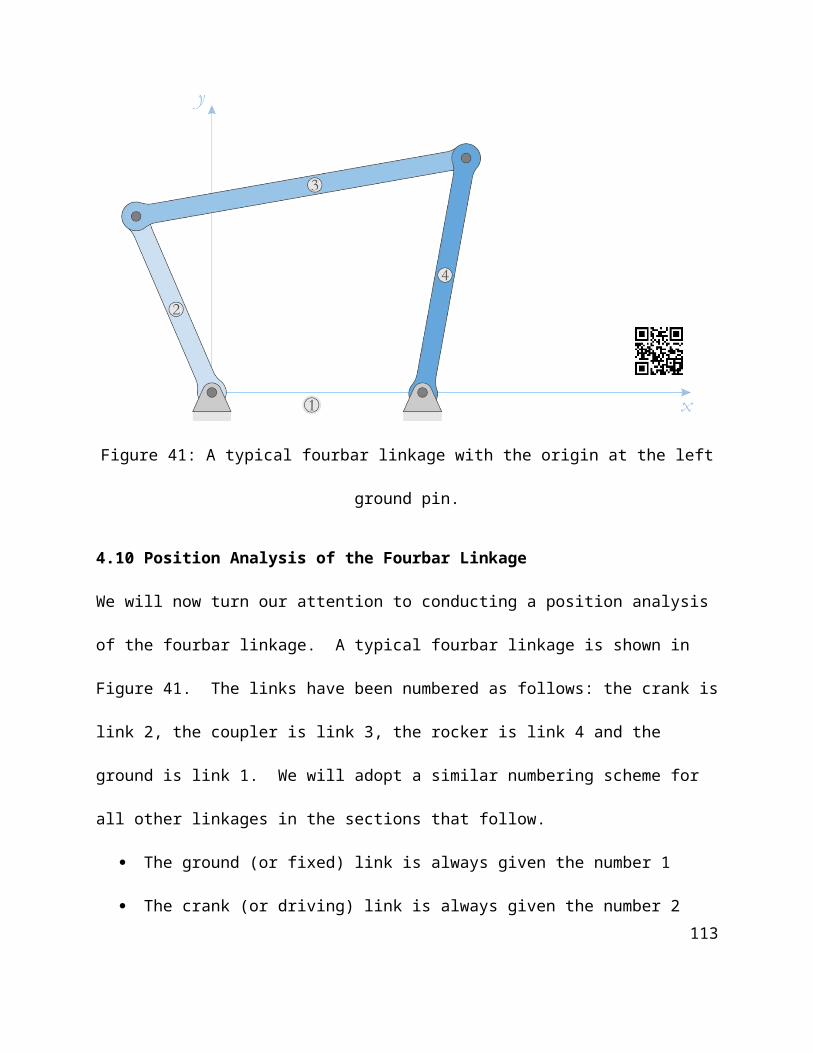
Figure 57: Paths of the points B, C and P. This is the plot you should obtain by running the code
described above. Your colors will be different than the plot above, but the shapes of the traces
should be the same.
Making a Fancy Plot and Verifying your Code
When you execute the program described above, you should obtain a set of three curves as
shown in Figure 26. We have solved the problem as it was given in the problem statement, but
there are still a few things we should add to make the plot more professional. You can copy and
paste many of the plot commands from the threebar position analysis program, with a few tweaks
to make it work for the fourbar.113

% specify angle at which to plot linkagehold oniTheta = 120; % plot the coupler as a triangular patchpatch([xB(1,iTheta) xC(1,iTheta) xP(1,iTheta)],... [xB(2,iTheta) xC(2,iTheta) xP(2,iTheta)],[229/255 240/255 249/255]); % plot crank and rockerplot([x0(1) xB(1,iTheta)],[x0(2) xB(2,iTheta)],'Linewidth',2,'Color','k');plot([xD(1) xC(1,iTheta)],[xD(2) xC(2,iTheta)],'Linewidth',2,'Color','k'); % plot joints on linkageplot([x0(1) xD(1) xB(1,iTheta) xC(1,iTheta) xP(1,iTheta)],... [x0(1) xD(2) xB(2,iTheta) xC(2,iTheta) xP(2,iTheta)],... 'o','MarkerSize',5,'MarkerFaceColor','k','Color','k'); % plot the labels of each jointtext(xB(1,iTheta),xB(2,iTheta)+.015,'B','HorizontalAlignment','center');text(xC(1,iTheta),xC(2,iTheta)+.015,'C','HorizontalAlignment','center');text(xP(1,iTheta),xP(2,iTheta)+.015,'P','HorizontalAlignment','center'); axis equalgrid on title('Paths of points B, C and P on Fourbar Linkage')xlabel('x-position [m]')ylabel('y-position [m]')legend('Point B', 'Point C', 'Point P','Location','SouthEast')
The purpose of most of this code, recall, is to make a “snapshot” of the linkage at a single crank
angle (in this case, 120°) so that we have an initial verification that the position analysis code is
working correctly. Figure 27 shows the final position plot of the fourbar linkage used in the
example.
114

Figure 58: Fourbar position plot with title, legend and axis labels and snapshot.
Plotting the Non-Grashof Linkage
The code given above will generate a plot for Grashof linkages only. Now consider the case
where the crank length is 150mm, the coupler is 200mm, the rocker is 170mm and the distance
between ground pivots is 250m. Here we have
S+L=400 mmP+Q=370 mm
so that the linkage is clearly non-Grashof. If we use these lengths in our code it will inform us
that the linkage is non-Grashof and will terminate without producing a plot. It is likely,
however, that we would prefer that the code produce position plots for the linkage in its possible
115

range of motion, even if the crank cannot undergo a full revolution.
Figure 59: Limits of motion for the non-Grashof linkage.
As seen in Figure 59, the linkage binds up when the coupler and rocker are aligned. We can use
the Law of Cosines to determine the angles θ2min and θ2max, which will define the range of motion
for the crank.
cosθ2max=a2+d2− (b+c )2
2ad(129)
Of course, θ2min is the negative of θ2max. If the linkage is Grashof, we would like the code to plot
the motion of the linkage for a full revolution of the crank. If it is not Grashof, we wish to plot
the resulting motion when the crank swings between θ2min and θ2max. Therefore, we must first
modify our Grashof condition checking logic as follows:
if (S+L < PQ) % Grashof condition
116

disp('Linkage is Grashof.') theta2min = 0; theta2max = 2*pi;else % if not Grashof, calculate range of motion disp('Linkage is not Grashof') theta2max = acos((a^2 + d^2 - (b + c)^2)/(2*a*d)); theta2min = -theta2max;end
Next, we must modify our calculation of θ2 in the main loop. For either case, we wish θ2 to
range between θ2min and θ2max. We can use a linear interpolation formula to effect this
θ2 ( i )=( θ2max−θ2 min
N−1 ) ( i−1 )+θ2 min
(130)
The reader should verify that the formula produces theta2 = theta2min when i = 1 and
theta2 = theta2max when i = N. Modify your theta2 calculation in the main loop as
theta2 = (i-1)*(theta2max - theta2min)/(N-1) + theta2min;
One disadvantage of this method is that the index, i, no longer corresponds directly to the crank
angle, theta2, so you must use Equation (130) to calculate the crank angle for a given index.
117

Figure 60: Plot of the non-Grashof linkage at iTheta = 200.
If you execute the code with iTheta set to 200 (crank angle 14.12°) you should obtain the plot
shown in Figure 60. Thus, we now have a MATLAB script that can plot the full range of motion
for both Grashof and (some) non-Grashof linkages.
118

Figure 61: Another type of non-Grashof linkage with the coupler as the longest link.
The linkage shown in Figure 59 has the ground as the longest link, and our code will plot the
motion of this type of non-Grashof linkage. In Figure 61 we see a non-Grashof linkage with the
coupler as the longest link, and whose limiting positions are quite different. It is left as an
exercise for the reader to modify the MATLAB code to account for this type of non-Grashof
119

linkage (hint: use an if statement to check which link is the longest, and calculate θ2min and θ2max
accordingly.)
Figure 62: The inverted slider-crank consists of a crank, slider, rocker and ground. The rocker
and slider are connected with a full-slider joint.
4.12 Position Analysis of the Inverted Slider-Crank
The next linkage in our program of study is the inverted slider-crank, shown in Figure 62. As
with the previous two linkages, the inverted slider-crank has four bars: crank, slider, rocker and
ground. The major difference between this linkage and the slider-crank is that the slider rides in
a moving slot, which is attached to the end of the rocker. Thus, the angle of the slot changes as
the rocker rotates. In general, the slot may make any angle, δ, with the rocker, but this angle
must remain constant. Given the obvious differences between the fourbar linkage and the
inverted slider-crank, position analysis of the two linkages will prove to be remarkably similar.
120

Figure 63: Dimensions of the inverted slider-crank linkage. The distance between points B and
C is defined as b, which changes as the linkage moves.
Figure 63 shows the dimensions of the inverted slider-crank. The crank length is a, the rocker
length is c, and the distance between ground pins is d. The point C is defined as the intersection
of the slider and the rocker. This point will travel up and down the slider as the linkage moves,
which will cause the length b to change with time. The angle between slider and rocker is
defined as δ. Recall that the fourbar linkage had four fixed lengths: a, b, c and d, and the angle
between coupler and rocker was variable. In contrast, the inverted slider-crank as fixed lengths
a, c and d, and a fixed angle δ, while the length b is variable. Following a similar line of
reasoning as with the fourbar, we can write:
121

θ4=θ3+δ (131)
Thus, we can easily find θ4 once we have found θ3 since δ is known. For the inverted slider-
crank, then, the list of known quantities is
known :a , c , d , δ , θ2
and the list of unknowns is
unknown : b ,θ3
Figure 64: The prime diagonal stretches from the crank pin to the ground pin of the rocker, as
with the fourbar.
122

We begin by drawing the prime diagonal, f as shown in Figure 64. We also define the quantities
r and s
r=d−acos θ2
s=a sin θ2
(132)
Using the Pythagorean Theorem, we find again that:
f 2=a2+d2−2ad cosθ2 (133)
We can make use of the Law of Cosines with the angle δ
f 2=b2+c2−2bc cosδ (134)
Everything in Equation (134) is known except the distance b. Let us rearrange this equation to
put it into a more familiar form
b2−(2 ccos δ ) b+(c2−f 2)=0 (135)
This is a quadratic equation in b, so we can use the quadratic formula to solve it
b=2c cosδ ±√4 c2cos2δ−4 (c2−f 2 )
2(136)
Using the trigonometric identity
cos2δ +sin2 δ=1 (137)
and factoring like terms out from the under the root, we can simplify this expression to
b=c cosδ ±√ f 2−c2sin2 δ (138)
123

Figure 65: The lengths g and h are defined by dropping a perpendicular line from the slider
through pin D.
We also define the quantities g and h, by drawing a perpendicular from the slider through pin D.
g=b−ccos δ
h=c sin δ
(139)
The formula for b then simplifies to
b=c cosδ ±√ f 2−h2 (140)
and once we have solved for b, we can calculate g. Finally, we can calculate the angle θ3 just as
we did for the fourbar
124

tanθ3=hr−gsgr+hs
(141)
Figure 66: The open and crossed configurations of the inverted slider-crank are found by taking
the two different solutions for the length b.
You might be wondering how to interpret the ± symbol in Equation (140). It comes about
because there are two different ways to assemble the inverted slider-crank, as shown in Figure
66. The assembly on the left is known as the the open configuration, since none of the lines
cross. The other configuration is called crossed. In the crossed configuration, the value for b is
negative, which means that the slider points in the direction opposite from the way its angle is
defined. Both are valid configurations for the linkage, but we usually are more interested in the
open configuration.
125

Limiting Positions for the Inverted Slider-Crank
Owing to the fact that the slider and rocker must meet at a specified angle, δ, it is more
challenging to assemble a working inverted slider-crank than it is for the fourbar or slider-crank.
To determine the viability of a given set of link lengths, let us first examine Equation (138),
which determines the length of the slider between the crank pin and the rocker.
b=c cosδ ±√ f 2−c2sin2 δ
In order to obtain a valid solution, the argument inside the radical must be positive (or zero).
Using Equation (133), the argument inside the radical can be expanded to
a2+d2−2ad cosθ2−c2 sin2δ ≥0 (142)
or
a2+d2−2ad cosθ2≥ c2sin 2δ (143)
Evaluating this inequality at its maximum and minimum values will determine the lengths of
links a, c and d that will allow the linkage to be constructed. The quantity on the left-hand side of
the equation takes on a maximum value when θ2 = 180°, and cos θ2 = -1, so that
a2+d2+2ad ≥ c2 sin2 δ (144)
Collecting the three terms on the left gives
(a+d )2≥ c2sin 2δ (145)
126

Figure 67: In the top figure the combined length of a and d are greater than c sin δ, so the
linkage can be assembled. In the bottom figure a + d < c sin δ so the linkage cannot be
assembled.
And taking the square root
|a+d|≥ c sin δ (146)
If this condition is not met, then the linkage cannot be assembled. In this situation, the rocker is
127

too long so that there is no configuration that the coupler can pass through the slider at the end of
the rocker.
Even if the linkage can be assembled, it is still possible for it to be “non-Grashof”; that is, the
crank may not be able to make a full revolution. Evaluating the minimum value of Equation
(143) when θ2 = 0, and cos θ2 = 1:
a2+d2−2ad cosθ2≥ c2sin 2δ
Factoring and simplifying as before, we find that
|a−d|≥ c sin δ (147)
If this condition is not met, then the crank cannot make a full revolution.
Figure 68: If (a – d) = c sinδ then the length b will be zero when θ2 = 0, causing a collision
between the rocker and crank if δ = 0.
If we barely meet the condition by setting the two sides of the equation equal to each other
|a−d|=c sin δ (148)
then b can equal zero if δ = 90. This is also an undesirable situation since it means that the crank
will collide with the rocker when θ2 = 0 (see Figure 68).
128

Figure 69: Limiting positions for the "non-Grashof" inverted slider-crank.
The limiting positions for the crank are found by setting the argument under the radical equal to
zero in Equation (138).
cosθ2=a2+d2−c2 sin2 δ
2ad(149)
The limiting angles are shown in Figure 69. It is interesting to note that we have once again
arrived at the law of cosines. When the linkage is at its limiting positions a triangle can be
constructed with sides a, d and c sinδ. As can be seen in Figure 69, the length b takes on the
value c cosδ in the limiting position, which is confirmed by Equation (138). It is a good idea to
check for the “Grashof” condition of the linkage in your code before starting the position
calculations.
129

Figure 70: Example inverted slider-crank linkage used in the MATLAB code.
4.13 Position Analysis of the Inverted Slider-Crank Using MATLAB
The code we develop for the inverted slider-crank will be very similar to the fourbar code. In
fact, you might wish to use Save As instead of retyping the entire program. The example linkage
130

used here is shown in Figure 70. This linkage is “Grashof”; that is, its crank can make a full
revolution. We will check the Grashof condition in order to be able to plot non-Grashof inverted
slider-cranks at the end of this section.
Enter the dimensions and allocate space for the variables as below
% InvSlider_Position_Analysis.m% Conducts a position analysis of the inverted slider-crank linkage and% plots the positions of points B, C and P% by Eric Constans, June 5, 2017 % Prepare Workspaceclear variables; close all; clc; % Linkage dimensionsa = 0.080; % crank length (m)c = 0.130; % rocker length (m)d = 0.200; % length between ground pins (m)p = 0.350; % slider length (m)delta = 60*pi/180; % angle between slider and rocker (converted to rad)h = c*sin(delta); % h is a constant, only calculate it once % ground pinsx0 = [0;0]; % ground pin at A (origin)xD = [d;0]; % ground pin at D
Note that the length h is a constant, and does not change with crank angle. Since it only needs to
be calculated once, we enter its formula before the main loop. We now enter the formulas
learned in the previous section inside the main loop.
for i = 1:N theta2(i) = (i-1)*(2*pi)/(N-1); r = d - a*cos(theta2(i)); s = a*sin(theta2(i)); f2 = r^2 + s^2; % f squared b(i) = c * cos(delta) + sqrt(f2 - h^2); g = b(i) - c*cos(delta); theta3(i) = atan2((h*r - g*s),(g*r + h*s)); theta4(i) = theta3(i) + delta; % calculate unit vectors [e2,n2] = UnitVector(theta2(i));
131

[e3,n3] = UnitVector(theta3(i)); [e4,n4] = UnitVector(theta4(i)); % solve for positions of points B, C and P on the linkage xB(:,i) = FindPos( x0,a,e2); xC(:,i) = FindPos( xD,c,e4); xP(:,i) = FindPos(xB(:,i),p,e3);end
Most of this code, with the exception of the b calculation, are familiar from the fourbar code.
Finally, modify the plotting commands to plot the links, and point P, of the inverted slider-crank.
plot(xB(1,:),xB(2,:),xC(1,:),xC(2,:),xP(1,:),xP(2,:))hold on
% specify angle at which to plot linkageiTheta = 120; % plot crank, slider and rockerplot([ x0(1) xB(1,iTheta)],[ x0(2) xB(2,iTheta)],... 'Linewidth',2,'Color','k');plot([xB(1,iTheta) xP(1,iTheta)],[xB(2,iTheta) xP(2,iTheta)],... 'Linewidth',2,'Color','k');plot([xD(1) xC(1,iTheta)],[xD(2) xC(2,iTheta)],... 'Linewidth',2,'Color','k'); % plot joints on linkage plot([x0(1) xD(1) xB(1,iTheta) xC(1,iTheta) xP(1,iTheta)],... [x0(2) xD(2) xB(2,iTheta) xC(2,iTheta) xP(2,iTheta)],... 'o','MarkerSize',5,'MarkerFaceColor','k','Color','k'); % plot the labels of each jointtext(xB(1,iTheta),xB(2,iTheta)+.015,'B','HorizontalAlignment','center');text(xC(1,iTheta),xC(2,iTheta)+.015,'C','HorizontalAlignment','center');text(xP(1,iTheta),xP(2,iTheta)+.015,'P','HorizontalAlignment','center'); axis equalgrid on title('Paths of points B, C and P on Inverted Slider-Crank')xlabel('x-position [m]')ylabel('y-position [m]')legend('Point B', 'Point C', 'Point P','Location','SouthEast')
132

Figure 71: Position plot for the example inverted slider-crank linkage.
The plot in Figure 71 shows the paths of important points on an inverted slider-crank as the
crank makes a full revolution. Use this plot to check the results of your own code before
attempting the homework problems.
Position Analysis of the non-Grashof Linkage
If you change the crank length to 100mm, you will have created a “non-Grashof” inverted slider
crank, since
|a−d|=100 mm
c sin δ=113mm
(150)
Since the condition133

|a−d|≥ c sin δ (151)
is not met, the crank cannot make a full revolution. As we did with the fourbar, let us check the
condition of the linkage at the beginning of the code, right after defining the link lengths. We
should first check if the linkage can be assembled at all, using the condition
a+d ≥ c sin δ (152)
If this condition is not met, we should terminate the program and return control to the command
window. If it is met, we should then check whether or not the linkage is Grashof. Enter the
following lines of code after the definitions of the link lengths
if ((a + d) < c*sin(delta)) disp('Linkage cannot be assembled') returnelse if (abs(a - d) >= c*sin(delta)) disp('Linkage is Grashof') theta2min = 0; theta2max = 2*pi; else disp('Linkage is not Grashof') theta2min = acos((a^2 + d^2 - (c*sin(delta))^2)/(2*a*d)); theta2max = 2*pi - theta2min; endend
134

Figure 72: Lower and upper limits of the crank angle, θ2, for the non-Grashof inverted slider-
crank
We use the check on the Grashof condition to define minimum and maximum values for
theta2. You have probably noticed that the definition of theta2min and theta2max are
slightly different than they were for the fourbar. This is because the crank starts its motion at an
angle theta2min above the horizontal and sweeps counterclockwise until it reaches
theta2max. To ensure that theta2max is greater than theta2min, we have used
θ2 max=2 π−θ2 min (153)
Be sure that the definition of theta2 inside the loop is
theta2(i) = (i-1)*(theta2max - theta2min)/(N-1) + theta2min;
After entering these lines of code, and changing a to a length of 100mm try running the code.
135

The classic MATLAB “ping” lets you know that you have encountered an error. When you
switch to the command line window you are greeted with the message:
Linkage is not GrashofError using atan2Inputs must be real.
Error in InvSlider_Position_Analysis (line 50) theta3(i) = atan2((h*r - g*s),(g*r + h*s));
It appears that one of the arguments in the atan2 function is imaginary. To find out which one
is the culprit, type each argument (followed by the enter key) at the command line.
>> hh = 0.1126>> rr = 0.1067>> gg = 0.0000e+00 + 1.8626e-09i>> ss = 0.0360
Everything looks as expected except for the variable g. The formula for g is
g=b−c sin δ (154)
Since c and sin δ are both real, we know that the problem must lie with b. Type b(1) at the
command line to look at a single calculated value within the b vector
>> b(1)ans = 0.0650 + 0.0000i
It appears as though b has a small (but finite) imaginary component. Since we calculated b using
the square root function,
136

b=c cosδ+√ f 2−h2 (155)
a slight roundoff error must have made h2 greater than f2. It is relatively straightforward to prove
that the quantity f2 – h2 should be zero at θ2min such that b = c cos δ. Instead, a slight numerical
error in calculating θ2min has caused b to have an imaginary component, which results in an error
in implementing the atan2 function. If MATLAB’s calculated value for θ2min is less than the
true value by even a tiny amount, b will end up with an imaginary component. A quick and easy
solution to this problem is to add a very small amount to θ2min (and subtract the same amount
from θ2max) to ensure that θ2 stays within bounds. Immediately after defining the link lengths, add
the statement
eps = 0.000001; % tiny number added to theta2 to keep it in bounds
Then change the formula for theta2min to the following
theta2min = acos((a^2 + d^2 - (c*sin(delta))^2)/(2*a*d)) + eps;
137

Figure 73: Position plot for the non-Grashof inverted slider-crank linkage in the example.
When you run the code again, the error should be gone, and you will be rewarded with the
position plot shown in Figure 73. We now have a general-purpose program to calculate the
positions of points on a Grashof and non-Grashof inverted slider-crank linkage. Be sure that
your plot matches Figure 73 before moving on.
138

Figure 74: The geared fivebar linkage has two gears, two couplers, a crank and a rocker. The
crank is attached to the first gear and the rocker is attached to the second gear.
4.14 Position Analysis of the Geared Fivebar Linkage
We now turn our attention to a slightly more complicated linkage, the geared fivebar. As shown
in Figure 74, the geared fivebar consists of two gears, two couplers, a crank and a rocker. The
crank is rigidly attached to the first gear and must rotate with it. The rocker is attached to the
second gear and must rotate with it as well. The two gears are in mesh so that the rotation of the
second gear is proportional to that of the first. We assume that the input to the linkage is the
rotation of the first gear. A quick degree-of-freedom analysis will reassure us that the geared
fivebar has only one degree of freedom, as required. The gear constraint removes one degree of
139

freedom (rotation) from the second gear and there are five pin joints. Using the modified
Gruebler Equation we find that
DOF=3 (5−1 )−2 (5 )−1=1 (156)
As before, we wish to find the location of any point on the linkage for a given input crank angle.
Figure 75: Dimensions of the geared fivebar linkage.
Figure 75 shows the important dimensions of the geared fivebar linkage. The crank has length a
and the first coupler has length b. The second coupler has length c, while the rocker has length
u. The distance between ground pins is d. Suppose that the first gear has N1 teeth and the second
gear has N2 teeth. Then the relationship between θ5 and θ2 is
θ5=−N1
N2θ2+φ
(157)
where φ is a constant offset angle that arises because we may place the two gears into mesh in
140

any manner we choose. For example, we may decide to assemble the linkage with the crank
oriented horizontally and the rocker oriented vertically: this would produce an offset angle of
φ=90°. The ratio N1/N2 is the gear ratio for the linkage – we shall have much more to say about
gear ratios in a later chapter. The negative sign arises from the fact that meshing external gears
rotate in opposite directions.
Assume, as always, that the link lengths are given. Since we have established a simple
relationship between θ2 and θ5, the list of knowns is
known :a , b , c ,d , u ,θ2, θ5 (158)
and the list of unknowns is
unknown :θ3, θ4 (159)
as it was for the fourbar linkage.
Figure 76: A line has been drawn from point A to point C. The links a, b, c and d' form a fourbar
linkage.141

Now examine Figure 76 above. We have drawn a diagonal line from the point A to the point C.
This line has length d' and makes an angle β with the horizontal. Since the angle θ5 is known, it
is simple to calculate the coordinates of point C.
xC=d e1+u e5 (160)
The length d' can be found using the Pythagorean theorem
d '=√( d+ucosθ5 )2+(u sin θ5 )2 (161)
Or
d '=|xC|=√xCx2 +xCy
2 (162)
and the angle β is seen to be
tan β=xCy
xCx
(163)
If we rotate our frame of reference by the angle β, the links a, b, c and d' form a simple fourbar
linkage whose solution is known from the previous section. Note that we must use a slightly
modified crank angle, θ'2 as the input to the solution procedure, to account for the fact that we
have rotated an angle β from the horizontal
θ2' =θ2−β (164)
We can use the fourbar formulas from earlier to solve for a modified coupler angle, θ'3, and then
rotate this back into the original coordinate frame by noting that
θ3=θ3' +β (165)
In other words, you may reuse almost all of the MATLAB code developed in Section 4.4 to
conduct the position analysis for the geared fivebar linkage! Of course, the length d' and the
angle β change with every crank angle so that these calculations must be placed inside the main 142

loop.
Figure 77: The geared fivebar linkage used in the first example
4.15 Position Analysis of the Geared Fivebar Using MATLAB
We will now implement the formulas we have learned into a MATLAB code for plotting the
positions of all points on the geared fivebar linkage. Figure 77 shows the example linkage we
143

will consider. Begin, as usual, with the initial comments and definitions of link lengths:
% Fivebar_Position_Analysis.m% conducts a position analysis on the geared fivebar linkage and% plots the positions of points P and Q% by Eric Constans, June 6, 2017 % Prepare Workspaceclear variables; close all; clc; % Linkage dimensionsa = 0.120; % crank length (m)b = 0.250; % coupler 1 length (m)c = 0.250; % coupler 2 length (m)d = 0.180; % distance between ground pins (m)u = 0.120; % length of link on gear 2 (m)N1 = 24; % number of teeth on gear 1N2 = 24; % number of teeth on gear 2rho = N1/N2; % gear ratiophi = 0; % offset angle between gearsgamma3 = 20*pi/180; % angle to point P on coupler 1gamma4 = -20*pi/180; % angle to point Q on coupler 2p = 0.200; % distance to point P on coupler 1q = 0.200; % distance to point Q on coupler 2
% ground pinsx0 = [0;0]; % ground pin at A (origin)xD = [d;0]; % ground pin at D % Main LoopN = 361; % number of times to perform position calculations[xB,xC,xE,xP,xQ] = deal(zeros(2,N)); % allocate space for positions[theta2,theta3,theta4] = deal(zeros(1,N)); % allocate space for angles
To keep things simple at first, we will let the numbers of teeth in the two gears be equal at 24.
Once we have developed and verified a working code, we will change the number of teeth in the
first gear to 48. Note that we have not allocated space for theta5, since
θ5=−ρ θ2 (166)
it can be easily calculated at any time. The internal angle of the coupler on the left is set to
positive 20° since we rotate counterclockwise from the line BE to BP. The second coupler has a
negative angle since we rotate -20° from the line CE to CQ.
144

for i = 1:N theta2(i) = (i-1)*(2*pi)/(N-1); % crank angle theta5 = -rho*theta2(i) + phi; % angle of second gear [e2,n2] = UnitVector(theta2(i)); % unit vector for crank [e5,n5] = UnitVector(theta5); % unit vector for second gear xC(:,i) = FindPos(xD, u, e5); % coords of pin C dprime = sqrt(xC(1,i)^2 + xC(2,i)^2); % distance to pin C beta = atan2(xC(2,i),xC(1,i)); % angle to pin C
Next, begin typing the main loop, as shown above. To conduct the position analysis, we must
first determine dprime and beta, which are calculated using the coordinates of point C. Since
we need the unit vector for link 5 in the calculation of xC, we calculate e2 and e5 as soon as the
angles theta2 and theta5 are known. The remainder of the main loop is very similar to that
of the fourbar position analysis, except that the angles must be modified by beta.
r = dprime - a*cos(theta2(i) - beta); s = a*sin(theta2(i) - beta); f2 = r^2 + s^2; % f squared delta = acos((b^2+c^2-f2)/(2*b*c)); g = b - c*cos(delta); h = c*sin(delta); theta3(i) = atan2((h*r - g*s),(g*r + h*s)) + beta; theta4(i) = theta3(i) + delta; [e3,n3] = UnitVector(theta3(i)); % unit vector for first coupler [e4,n4] = UnitVector(theta4(i)); % unit vector for second coupler [eBP,nBP] = UnitVector(theta3(i) + gamma3); % unit vec from B to P [eCQ,nCQ] = UnitVector(theta4(i) + gamma4); % unit vec from C to Q xB(:,i) = FindPos( x0, a, e2); xE(:,i) = FindPos(xB(:,i), b, e3); xP(:,i) = FindPos(xB(:,i), p, eBP); xQ(:,i) = FindPos(xC(:,i), q, eCQ); end
145

Figure 78: There are two paths to point C, which can be used as a means of verifying the fivebar
code.
Verifying your code
Of course, no simulation is complete without some form of code verification. As discussed
earlier, quick way to check your results is to make a sketch of the linkage in SolidWorks
(without the gears) and see if the coordinates produced by your code match the ones in the
sketch. A second method of verification is to note that there are two vector paths to the point E,
as shown in Figure 78.
r E=ae2+b e3r E=d e1+u e5+c e4 (167)
As a first check on the accuracy of your code, create a plot of the trajectory of point E calculated
in both of the ways given in Equation (167). If both traces are exactly alike, then you can have
some confidence that your code is producing accurate results.
146

Figure 79: Trajectory of point E for the example fivebar with gear ratio = 1. Both methods for
reaching point E produce the same trace.
As seen in Figure 79 both methods for reaching point E produce the same result. The resulting
curve resembles the symbol for infinity or a sideways figure eight, and is known as a lemniscate.
147

Figure 80: Finding the coordinates of the points P and Q on the geared fivebar.
Position of any point on the linkage
As with the fourbar linkage, we may be interested in the trajectory of a point on the fivebar that
is not located at a pin joint. In Figure 80 we have a diagram showing vector paths to two points,
P and Q. Both of the couplers are represented as triangles in this diagram, to show that they may
have arbitrary shape. Note that γ4 is negative as shown in the figure, since it represents a
clockwise rotation. The vector path to points P and Q are
xP=r2+rBP
xQ=r1+r5+rCQ
(168)
or, using unit vector notation
xP=a e2+ p eBP (169)
148

xQ=de1+ue5+q eCQ (170)
The following section contains a few plots of sample geared fivebar linkages. Try to get your
code to match these results before tackling any of the geared fivebar homework problems.
Figure 81: Paths of points P and Q for the example linkage with gear ratio = 1.
Example 1: Gears with equal numbers of teeth
Figure 81 shows the trajectory of points P and Q for the example linkage with equal numbers of
teeth. It is perhaps not surprising that the curves are symmetric, since the linkage is symmetric
and both gears are identical.
149

Figure 82: Paths of points P and Q with gear 1 = 48 teeth and gear 2 = 24 teeth.
Example 2:Gears with unequal numbers of teeth.
Figure 82 shows the trajectory of points P and Q for the example fivebar with gear 1 having 48
teeth and gear 2 having 24 teeth. Note the presence of several cusps in the trajectories. A cusp
(or “tooth”) is a location where a point on the linkage changes direction suddenly – this will
provide some interesting challenges when we conduct velocity and acceleration analysis. Even a
very simple linkage can generate complicated paths!
150

Figure 83: Stephenson Type I sixbar linkage.
Figure 84: Stephenson Type II sixbar linkage
151

Figure 85: Stephenson Type III sixbar linkage.
Figure 86: Watt Type I sixbar linkage.
152

Figure 87: Watt Type II sixbar linkage.
4.16 Position Analysis of the Sixbar Linkage
As the final mechanism in our study of position analysis we will examine the one degree of
freedom sixbar linkage. There are five types of 1 DOF sixbar linkage, as shown in Figure 83
through Figure 87. Each linkage consists of four two-pin links and two three-pin links. In the
Stephenson linkages the three-pin links are separated by the two-pin links (two single links and
one two-link pair), while in the Watt linkages the three-pin links are directly connected, and the
two-pin links are connected in pairs. The types are distinguished by which link is grounded.
As we will see, four of the five sixbar linkages can easily be analyzed by first solving the fourbar
problem for the lower set of links and then finding the angles of the remaining two links using
another fourbar position analysis. Only the Stephenson Type II sixbar resists solution using this
method, since its lower linkage chain consists of five bars.
153

Figure 88: Dimensions of the Stephenson Type I sixbar linkage. The links a, b, c and d form a
fourbar linkage.
154

Figure 89: The upper “virtual” fourbar linkage is formed by aʹ, u, v and dʹ.
Stephenson Type I Sixbar Linkage
Figure 88 shows the critical dimensions of the Stephenson Type I sixbar linkage. Here we
assume that link ABE is the crank and link AD is the ground. The links of dimension a, b, c and
d form a fourbar, and the angles θ3 and θ4 can be found using the ordinary fourbar solution
developed earlier. Now observe that points BEGF form a second, “virtual” fourbar linkage on
top of the first. As shown in Figure 89 the “virtual crank” has length aʹ, the “virtual ground” has
length dʹ, the “virtual coupler” has length u and the “virtual rocker” has length v. The lengths u
and v are constant, and are given in the problem statement, of course.
To find the lengths aʹ and dʹ, it is helpful to determine the coordinates of a few key points on the
155

linkage. Assume that we have conducted the fourbar position analysis for the linkage given by
ABCD, so that the angles θ3 and θ4 are known. The points B and E are attached to the three-pin
crank, and their coordinates are
xB=ae2 (171)
xE=p eAE (172)
The point F is attached to the three-pin rocker, and its coordinates are
xF=d e1+q eDF (173)
Since the virtual link dʹ serves as the ground for the upper fourbar, the “virtual crank angle” θ2ʹ is
given by
θ2' =α−β (174)
where
tan α=y E− y B
x E−xB
(175)
and
tan β=y F− yB
x F−x B
(176)
The lengths of the virtual links aʹ and dʹ can be found using the Pythagorean theorem
a '=√ ( xE−xB )2+( y E− yB )2 (177)
d '=√( x F−xB )2+( y F− y B )2 (178)
Once the lengths of the virtual links and crank angle are known, the angles θ5ʹ and θ6ʹ can be
found using the ordinary fourbar procedure, with u and v in place of b and c. Since the ground
on the upper fourbar has been rotated an angle β from the horizontal, the angles of the upper two
bars must be adjusted as
156

θ5=θ5' +βθ6=θ6
' +β (179)
Figure 90: Critical dimensions of the Stephenson Type III sixbar linkage.
157

Figure 91: Critical dimensions of the Watt Type I sixbar linkage.
158

Figure 92: Critical dimensions of the Watt Type II sixbar linkage.
The remaining sixbar linkages
Analysis of the remaining sixbar linkages (with the exception of the Stephenson Type II sixbar)
proceeds as with the Stephenson Type I sixbar. First, the lower fourbar linkage is analyzed, and
the angles θ3 and θ4 are found. Then the angles in the upper “virtual” fourbar are found by
rotating the virtual ground by the angle β. The coordinates for critical points on the linkages
have been tabulated in Table 2. The important angles and lengths used in solving the virtual
fourbar linkage are seen in Table 3. A general solution procedure for the sixbar linkages is
shown below. Follow this procedure when developing your MATLAB code to conduct the
position analysis of the sixbar linkages.
159

1. Enter the link lengths a, b, c, d, p, q, u, v and the three-pin link internal angles γ as given
in the problem statement.
2. Main Loop
a. Use the lengths a, b, c and d, and the crank angle θ2 to conduct a position analysis
of the lower fourbar linkage. It is simplest to copy and paste your fourbar code
for this section.
b. Calculate the coordinates of pins B, C, D, E and F using the formulas given in
Table 2.
c. Calculate the angles α, β using the formulas in Table 3 and then compute the
virtual crank angle θ2ʹ using Equation (174).
d. Calculate the virtual crank length aʹ and virtual ground length dʹ using Table 3.
e. Use the lengths aʹ, u, v, dʹ and the virtual crank angle θ2ʹ in the fourbar solution
procedure to find the angles θ5ʹ and θ6ʹ.
f. Add the angle β to θ5ʹ and θ6ʹ to obtain the angles θ5 and θ6 in the fixed coordinate
system.
g. Compute the coordinates of point G.
3. Create plots of the desired points on the linkage.
In the next section we will use MATLAB to carry out the procedure described above. We will
develop a code for only one of the linkages (the Stephenson Type I sixbar) since the remaining
three are so similar. Only the Stephenson Type II sixbar cannot be analyzed using this method,
as described below.
160

Figure 93: Vector loop diagram of the Stephenson Type II sixbar linkage. This linkage cannot
be analyzed by algebraic means alone.
The Stephenson Type II sixbar linkage
As seen in Figure 84, the Stephenson Type II sixbar linkage does not contain a grounded fourbar.
Instead, the links 1, 2, 3, 4 and 5 form a grounded fivebar linkage, which cannot be solved using
the algebraic methods discussed thus far. Figure 93 shows a vector loop diagram of the linkage.
We may write two loop equations as given in the figure
r2+r3+r5−r4−r1=0r2+r3 E+r6−r4 F−r1=0 (180)
and the result will be four nonlinear, transcendental equations with four unknown angles, θ3, θ4,
θ5 and θ6. To solve these we may employ one of the nonlinear equation solvers in MATLAB, or
write a simple Newton-Raphson solver. The Newton-Raphson solver is discussed in the final
161

section of this chapter, and this method has been used to construct the animations of the
Stephenson Type II sixbar linkages on the website.
Summary
We have presented solution techniques for four of the five types of one degree of freedom sixbar
linkages. Each of these is based upon performing the fourbar linkage position analysis twice:
once for a grounded lower linkage and again for a “virtual” upper fourbar. MATLAB code is
given in the next section for the Stephenson Type I linkage, but you should try programming the
remaining linkages (and checking your answers with the plots in the next section) on your own.
Only the Stephenson Type II linkage defies solution using algebraic techniques. In the next
chapter we will use the position analysis codes developed here as a basis for performing velocity
analysis on the linkages. As we will see, velocity analysis is a simple extension of position
analysis.
Table 2: Coordinates of critical points on sixbar linkages.
Stephenson I Stephenson III Watt I Watt IIxB a e2 a e2 ae2 a e2
xC xB+b e3 xB+b e3 xB+b e3 xB+b e3
xD d e1 d e1 d e1 d e1
xE peAE xB+ peBE xB+ peBE xD+ pe DE
xF xD+q eDF q eAF xD+qeDF q eAF
xG xE+u e5 xE+u e5 xE+u e5 xE+u e5
Table 3: Important angles and crank and ground lengths of upper fourbar for the sixbar linkages.
Stephenson I Stephenson III Watt I Watt II
tan βyF− yB
xF−xB
yF− yC
xF−xC
yF− yC
xF−xC
yF− y D
xF−xD
162

tan αyE− yB
xE−xB
yE− yC
xE−xC
yE− yC
xE−xC
yE− yD
xE−xD
a ' √ ( xE−xB )2+( y E− yB )2 √ ( xE−xC )2+ ( yE− yC )2 √ ( xE−xC )2+ ( yE−C y )2√ ( xE−xD )2+( yE− yD )2
d ' √ ( xF−xB )2+( yF− yB )2 √ ( xF−xC )2+( yF− yC )2 √ ( xF−xC )2+( yF−C y )2√ ( xF−xD )2+ ( yF− y D )2
Figure 94: The Stephenson Type I sixbar linkage used in the example.
163

4.17 Position Analysis of the Sixbar Linkage Using MATLAB
We will now use the procedure developed in the preceding section to create a MATLAB script to
perform a position analysis on the Stephenson Type I sixbar linkage. This will be the most
complicated script we have developed so far, with more than 100 lines of code! It is worthwhile
to go through the development in some detail, so that writing the programs for the other sixbar
linkages will be relatively straightforward.
Figure 83 gives the dimensions of the sixbar linkage we will analyze. We will closely follow the
procedure outlined in the previous section. The top portion of the code is similar to the programs
we have already written; first define the link lengths and angles, then allocate space for the
position variables as shown in Step 1 of the procedure.
% Sixbar_S1_Position_Analysis.m% conducts a position analysis of the Stephenson Type I sixbar linkage% and plots the positions of points E, F and G.% by Eric Constans, June 2, 2017 % Prepare Workspaceclear variables; close all; clc; % Linkage dimensionsa = 0.070; % crank length (m)b = 0.100; % coupler length (m)c = 0.090; % rocker length (m)d = 0.110; % length between ground pins (m)p = 0.150; % length to third pin on crank triangle (m)q = 0.150; % length to third pin on rocker triangle (m)u = 0.120; % length of link 5 (m)v = 0.160; % length of link 6 (m)gamma2 = 20*pi/180; % internal angle of crank trianglegamma4 = -20*pi/180; % internal angle of rocker triangle % Ground pinsx0 = [ 0; 0]; % ground pin at A (origin)xD = [ d; 0]; % ground pin at D
% allocate space for variablesN = 361; % number of times to perform position calculations[xB,xC,xE,xF,xG] = deal(zeros(2,N)); % positions[theta2,theta3,theta4,theta5,theta6] = deal(zeros(1,N)); % angles
164

Since the lower fourbar linkage is composed of links with length a, b, c and d, we can copy the
fourbar position analysis code directly, as given in Step 2a.
% Main Loopfor i = 1:N % solve lower fourbar linkage theta2(i) = (i-1)*(2*pi)/(N-1); % crank angle r = d - a*cos(theta2(i)); s = a*sin(theta2(i)); f2 = r^2 + s^2; delta = acos((b^2+c^2-f2)/(2*b*c)); g = b - c*cos(delta); h = c*sin(delta); theta3(i) = atan2((h*r - g*s),(g*r + h*s)); % coupler angle theta4(i) = theta3(i) + delta; % rocker angle
We then use the formulas in Table 1 to calculate the coordinates of pins B, C, E and F, as
suggested by Step 2b. The location of pin D is fixed, and was calculated before the main loop.
% calculate unit vectors [e2,n2] = UnitVector(theta2(i)); [e3,n3] = UnitVector(theta3(i)); [e4,n4] = UnitVector(theta4(i)); [eAE,nAE] = UnitVector(theta2(i) + gamma2); [eDF,nDF] = UnitVector(theta4(i) + gamma4); % solve for positions of points B, C, E, F xB(:,i) = FindPos(x0,a, e2); xC(:,i) = FindPos(xD,c, e4); xE(:,i) = FindPos(x0,p,eAE); xF(:,i) = FindPos(xD,q,eDF);
Next we must calculate the angles α and β using the formulas given in Table 2, as well as the
virtual crank and ground lengths, aʹ and dʹ. Since these formulas require the repeated use of
differences in coordinates, it will save some computational effort (and make the code neater) to
define the temporary variables xFB, yFB, xEB and yEB.
% solve upper fourbar linkage xFB = xF(1,i) - xB(1,i); yFB = xF(2,i) - xB(2,i); xEB = xE(1,i) - xB(1,i); yEB = xE(2,i) - xB(2,i); beta = atan2(yFB, xFB);
165

alpha = atan2(yEB, xEB); aPrime = sqrt(xEB^2 + yEB^2); % virtual crank length on upper fourbar dPrime = sqrt(xFB^2 + yFB^2); % virtual ground length on upper fourbar theta2Prime = alpha - beta; % virtual crank angle on upper fourbar
As given in Step 2e, we now compute the angles in the upper fourbar linkage
r = dPrime - aPrime*cos(theta2Prime); s = aPrime*sin(theta2Prime); f2 = r^2 + s^2; delta = acos((u^2+v^2-f2)/(2*u*v)); g = u - v*cos(delta); h = v*sin(delta); theta5Prime = atan2((h*r - g*s),(g*r + h*s)); % coupler and rocker angles theta6Prime = theta5Prime + delta; % on upper fourbar
Finally, use the angle β to rotate back to the original coordinate system and solve for the
coordinates of point G.
theta5(i) = theta5Prime + beta; % return angles to fixed theta6(i) = theta6Prime + beta; % fixed CS % calculate remaining unit vectors [e5,n5] = UnitVector(theta5(i)); [e6,n6] = UnitVector(theta6(i)); % calculate position of point G xG(:,i) = FindPos(xE(:,i), u, e5); end
Making the Sixbar Plot
Because of the large number of links, the sixbar position plots will be somewhat crowded. To
make them more readable, we will introduce a few new plotting tricks here. First, it will be
handy to make use of more than the default eight MATLAB colors.
There are multiple methods for handling colors in MATLAB (see, e.g. colormap, etc.), but the
166

method presented here is simple to implement. It is common in computer systems to specify a
color using an “RGB triple” in the form [R G B] where R, G and B are values between 0 and 255
that give the red, green and blue content of a color, respectively. For example, pure red would be
given by the triple [255 0 0], white is [255 255 255] and medium gray is [128 128 128]. In our
system, we will define a base color, and use a MATLAB function to calculate the RGB triples
for ten shades of that color. The first shade will be the base color itself, and the remaining
shades will be progressively lighter until the final shade is almost white.
We will use a linear interpolation formula to calculate the RGB value for each shade. If the base
value for a given color is S0, then the formula for shade i is
Si=255−S0
10(i−1)+S0
(181)
The reader will confirm that the formula gives Si = S0 when i = 0 and Si=255 when i=11. Let us
create a function, DefineColor.m, to create our own custom palette of colors. Open up a
new script, and type the following function.
% DefineColor.m% makes a palette of custom colors for plotting in MATLAB% the first color in the palette gives the full base color, and% the rest fade gradually to white%% colorBase = 1x3 input array giving RGB values (between 0 and 255)% C = 10x3 output array giving RGB values (between 0 and 1) function C = DefineColor(colorBase) C = zeros(11,3);for i = 1:11 for j = 1:3 C(i,j) = (i-1)*(255 - colorBase(j))/10 + colorBase(j); endend C = C/255;
The final line in the function divides the entire array by 255, since MATLAB specifies its RGB
167

values in the range between 0 and 1. In the main program immediately after the end of the main
loop type
cBlu = DefineColor([ 0 110 199]); % Pantone 300CcBlk = DefineColor([ 0 0 0]); % grayscale
Figure 95: Color palette defined by the function DefineColor.m.
These lines define two color palettes: cBlu and cBlk that give shades of blue and grayscales,
respectively. Coincidentally, these are the palettes used for the illustrations in this textbook!
To plot the trajectories of points E, F and G, type
figure; hold onplot(xE(1,:),xE(2,:),'Color',cBlu(1,:))plot(xF(1,:),xF(2,:),'Color',cBlu(7,:))plot(xG(1,:),xG(2,:),'Color',cBlk(5,:))
Instead of using the default MATLAB colors, we have used our newly-defined palettes to
168

customize the traces. Next, plot the two triangular links, the crank and rocker:
iTheta = 120; % specify angle at which to plot linkage% plot the two three-pin links as triangular patchespatch([x0(1) xB(1,iTheta) xE(1,iTheta)],... [x0(2) xB(2,iTheta) xE(2,iTheta)],cBlu(9,:),... 'EdgeColor',cBlk(6,:),'LineWidth',2,'FaceAlpha',0.5);patch([xD(1) xF(1,iTheta) xC(1,iTheta)],... [xD(2) xF(2,iTheta) xC(2,iTheta)],cBlu(10,:),... 'EdgeColor',cBlk(6,:),'LineWidth',2,'FaceAlpha',0.5);
Since the triangular links are plotted after the traces, it is likely that some of the traces have been
obscured. To avoid this, we have used the FaceAlpha parameter to make the links
semitransparent. We have also made the edges a medium gray so that the traces will stand out.
% plot the two-pin linksplot([xB(1,iTheta) xC(1,iTheta)],[xB(2,iTheta) xC(2,iTheta)],... 'Linewidth',2,'Color',cBlk(5,:));plot([xE(1,iTheta) xG(1,iTheta)],[xE(2,iTheta) xG(2,iTheta)],... 'Linewidth',2,'Color',cBlk(5,:));plot([xF(1,iTheta) xG(1,iTheta)],[xF(2,iTheta) xG(2,iTheta)],... 'Linewidth',2,'Color',cBlk(5,:));
% plot fixed pins plot([x0(1) xD(1)],[x0(2) xD(2)],'o','MarkerSize',5,... 'MarkerFaceColor',cBlk(1,:),'Color',cBlk(1,:)); % plot joints on linkage plot([xB(1,iTheta) xC(1,iTheta) xE(1,iTheta) xF(1,iTheta) xG(1,iTheta)],... [xB(2,iTheta) xC(2,iTheta) xE(2,iTheta) xF(2,iTheta) xG(2,iTheta)],... 'o','MarkerSize',5,'MarkerFaceColor',cBlk(6,:),'Color',cBlk(6,:));
Plotting the two pin links and pin joints is the same as before, although we have changed the
color of the moving pins to medium gray.
% plot the labels of each jointtext(x0(1), x0(2) - 0.012, 'A','HorizontalAlignment','center');text(xD(1), xD(2) - 0.012, 'D','HorizontalAlignment','center');text(xB(1,iTheta),xB(2,iTheta)+0.012,'B','HorizontalAlignment','center');text(xC(1,iTheta)+0.012,xC(2,iTheta),'C','HorizontalAlignment','center');text(xE(1,iTheta)-
169

0.012,xE(2,iTheta),'E','HorizontalAlignment','center');text(xF(1,iTheta),xF(2,iTheta)+0.012,'F','HorizontalAlignment','center');text(xG(1,iTheta),xG(2,iTheta)+0.012,'G','HorizontalAlignment','center'); axis equalgrid ontitle('Paths of points E, F and G on S1 Sixbar Linkage')xlabel('x-position [mm]')ylabel('y-position [mm]')legend('Point E', 'Point F', 'Point G','Location','SouthEast')
Figure 96: Paths of E, F and G for the example Stephenson Type I sixbar linkage.
Finally, the commands for labeling the points are the same as we used for the previous linkages.
If you have entered everything correctly, you should obtain the position plot shown in Figure 96.
170

The remaining sixbar linkages
A MATLAB script that solves the Stephenson Type I linkage has been developed above.
Programs for the remaining sixbar linkages (with the exception of the Stephenson Type II) are
left as an exercise for the reader. Below are a set of example plots of the four types of sixbar
linkages that we have discussed. Ensure that your plots match these before beginning the
homework exercises!
Figure 97: Dimensions of example Stephenson Type III linkage. The internal angle of the
171

ground triangle is negative since it sweeps clockwise from the line between ground pivots.
Figure 98: Position solution for the example Stephenson Type III linkage
172

Figure 99: Dimensions of the example Watt Type I sixbar linkage.
173

Figure 100: Position solution for the Watt Type I linkage.
174

Figure 101: Dimensions of the example Watt Type II linkage. The internal angles of the ground
and rocker are negative since they sweep out in the clockwise direction.
175

Figure 102: Position solution for the example Watt Type II linkage.
4.18 Advanced Topic: The Newton-Raphson Method
We have seen in the preceding sections that there are some linkages whose positions cannot be
analyzed using algebraic methods, most notably the Stephenson Type II sixbar linkage. This
section presents a method for conducting the position analysis for any one DOF linkage: the
Newton-Raphson algorithm. In contrast with the algebraic methods presented so far, the
Newton-Raphson algorithm is iterative, which means that we use a “guess and check” approach
to finding the positions. This means that the Newton-Raphson algorithm will generally be
slower than the algebraic approach, if it is available. As we will see, our guesses will not be
176

completely random, and the algorithm usually converges on the correct solution after only a few
tries. And for some linkages (e.g. the Stephenson Type II sixbar) we have no choice but to use
an iterative approach.
Figure 103: Vector loop diagram for the fourbar linkage.
As a first example we will conduct a position analysis of the fourbar linkage, since its equations
are simpler than the sixbar. Consider the vector loop diagram shown in Figure 103. Adding the
vectors around the loop brings us back where we started, so that the vector sum is zero.
r2+r3−r4−r1=0 (182)
Expanding this equation into its x and y components gives
acosθ2+bcosθ3−ccosθ4−d=0a sin θ2+b sin θ3−c sinθ4=0 (183)
These equations are sometimes called constraint equations, since they must both be satisfied in
177

order for the linkage to be properly assembled. Both equations have the form
f (θ2 , θ3 , θ4 )=0 (184)
In other words, the left-hand sides of both equations are functions of θ2, θ3 and θ4, and both must
equal zero at all times. Since we normally specify the crank angle in advance, it is more correct
to write Equation (184) as
f (θ3 ,θ4 )=0 (185)
Let us denote the vector of unknowns in this equation as q
q={θ3
θ4} (186)
Since we have two equations of constraint which both must equal zero, we can also write this as
a vector in the form
Φ (q )=0 (187)
where
Φ1=acosθ2+b cosθ3−ccosθ4−dΦ2=a sin θ2+b sin θ3−csin θ4 (188)
The Newton-Raphson algorithm is a method for solving systems of nonlinear equations of the
type in Equation (187). We will first discuss how the method works with a single equation and
single unknown, and then generalize it for multiple equations and multiple unknowns.
The Newton-Raphson Algorithm for One Equation and One Unknown
Consider a single constraint equation of the form
Φ (q )=0 (189)
where Φ can be any function of q, for example
178

sin q=0q2=05q+3=0 (190)
In each case, we would like to solve for q such that the left hand side of the equation equals zero.
In other words, we are interested in finding the root of each equation. For the expressions above,
finding the roots is simple, but for more complicated equations, an analytical solution is not
always possible. For this type of equation, we need to develop an automatic procedure that we
can implement in MATLAB. The procedure we will use is the Newton-Raphson algorithm.
Figure 104: The initial guess in the Newton-Raphson algorithm
The simplest way to present the Newton-Raphson algorithm is graphically, as shown in Figure
104. The thick blue line shows Ф(q), a function of the variable q. Initially, we don’t know what
179

the function Ф looks like at all points (i.e., we do not really know enough about Ф to make the
plot above!) but we can make an initial guess, q1, and work from there. Again, our goal is to find
q*, the value of q that makes the function Ф zero.
Assume that our initial guess, q1, was not very good, as in Figure 104. We can deduce the best
direction to proceed by examining the slope (or derivative) of Ф at q1
slope= d Фdq |
q 1
(191)
In Figure 105, the slope tells us that a more fruitful place to search for q* would be at a lower
value of q. In fact, we can make a pretty good guess as to the location of q* by noting that the
points Ф(q1), q* and q1 form a triangle, whose base is (q1-q*), height is Ф(q1), and slope is
dФ/dq. Using this triangle, we can rewrite the slope at q1 as
d Фdq |
q1
≈Ф ( q1 )−0
q1−q¿
180

Figure 105: Direction to move for the second guess.
Solving this equation for q*, we have
q¿=q1−Φ ( q1 )d Φdq |
q1
(192)
This is the estimating procedure for the Newton-Raphson algorithm. If the constraint equation is
linear, we can find the root in one step! Of course, our linkage constraint equations are not
linear, and it will take multiple steps to find the roots.
181

Figure 106: More than one move is required for nonlinear functions.
If the equation is nonlinear, as shown in Figure 106, we can use Equation (192) to make a guess
at q*, and iterate until we find it to sufficient accuracy. Starting at point q1, we find q2
q2=q1−Φ (q1)dΦdq |
q1
(193)
If this point is close enough to q*, we stop there. Otherwise we keep estimating until we have
converged upon q*.
182

q i+1=qi−Φ (qi )d Φdq |
qi
(194)
One Dimensional Examples
Let us try a few examples to become familiar with the algorithm. We’ll start simple, and work
our way to more complicated functions. First, consider the following linear function:
Φ=2 q+3 (195)
We wish to find the value of q that makes the function Φ equal to zero. To start the algorithm,
we make an initial (random) guess.
guess :q1=5 (196)
If we substitute this into the function Φ, we have
Φ (5 )=13 (197)
This isn’t anywhere near zero, so we need to update our guess using the Newton-Raphson
formula. To use the formula, we need to know the derivative of the function
d Φdq
= ddq
(2q+3 )=2 (198)
The next guess is then
q2=q1−Φ (q1)dΦdq |
q1
=5−132
=−32
(199)
Substituting this into our function, we see that
Φ (−32 )=2 ·(−3
2 )+3=0 (200)
Thus, with one guess, we have found the value of q that makes Φ zero. This is always the case
for linear functions.183

Figure 107: The cubic function used in the example. This function crosses the x axis at three
locations.
A more complicated function
Let us try something a little more complicated: a cubic function which has been plotted in Figure
107.
Φ=q3−q2−10 q (201)
The derivative of this function is
d Φdq
=3q2−2q−10 (202)
184

As an initial guess, let’s try
q1=5 (203)
as before. Substituting this into the function, we have
Φ (5)=50 (204)
Nowhere near zero! The derivative of the function at q = 5 is
d Φdq
(5)=55 (205)
The next guess is then
q2=q1−Φ (q1)d Φdq |
q1
=5−5055
=4.091(206)
If we substitute q = 4.091 into the function, we get
Φ (4.091)=10.819 (207)
We are getting closer! The derivative of the function at q = 4.091 is
dΦdq
(4.091)=32.025 (208)
The next guess is then
q3=q2−Φ (q2 )d Φdq |
q2
=4.091−10.81932.025
=3.753(209)
If we substitute q = 3.753 into our function, we get
Φ (3.753)=1.248 (210)
Much closer! Let’s try one last guess. The derivative of the function at q = 3.753 is
d Φdq
(3.753)=24.751 (211)
185

The next guess is then
q4=q3−Φ ( q3 )d Φdq |
q3
=3.753− 1.24824.751
=3.703(212)
The value of the function here is
Φ (3.703)=0.026 (213)
This is close enough to zero! Although this function was considerably more complicated than
the first one, it took us only four iterations to find the root. The root is q* = 3.703. The tables
below give examples of what happens when we try different initial guesses. Table 4 shows the
initial guess we just tried, q1 = 5.
Table 4: Initial guess = 5.0
i qi Φ dΦ/dq1 5.000 50.000 55.0002 4.091 10.819 32.0253 3.753 1.248 24.7514 3.703 0.026 23.7245 3.702 0.0000121
Next, we’ll try a smaller initial guess, q1 = 1.5. As you can see in Table 5, we have arrived at at
different root, q* = 0. Since our function is cubic, we can expect there to be three roots.
Table 5: Initial guess = 1.5.
i qi Φ dΦ/dq1 1.500 -13.875 -6.2502 -0.72 6.308 -7.0053 0.181 -1.832 -10.263
186

4 0.00203 -0.02 -10.0045 4.101×10⁻⁷ 4.101×10⁻⁶ -10.000
Next, we try an initial guess q1 = -1.5. As seen in Table 6, the algorithm has some difficulty in
converging to an answer. The reason for this is that the slope at q1 = -1.5 is very shallow (-0.25).
The updated guess is therefore very far away from the initial guess (q2 = 36). That is, because of
the shallow slope, we move very far away from the location of the roots. This is a danger in
using the Newton-Raphson algorithm - if our initial guess happens to lie at a point of zero slope,
the algorithm may have trouble converging.
Table 6: Initial guess = -1.5.
i qi Φ dΦ/dq1 -1.500 9.375 -0.252 36.000 45,000 38063 24.177 13,305 16954 16.328 3923 7575 11.146 1149 3406 7.771 331.145 155.6147 5.643 91.403 75.2388 4.412 22.280 39.5629 3.848 3.702 26.73410 3.710 0.1995 23.871
In our final example, shown in Table 7, we converge to the root -2.702. Convergence occurs
very quickly, in four or five iterations.
Table 7: Initial guess = -4.0.
i qi Φ dΦ/dq
187

1 -4.000 -40 462 -3.13 -9.172 25.663 -2.773 -1.282 18.6144 -2.704 -0.0439 17.3455 -2.702 -0.000058 17.298
Newton-Raphson in Multidimensional Space
We can use the same type of iterative procedure to solve multiple nonlinear equations
simultaneously. Our task now is to create a version of Equation (194) for multiple constraint
equations.
q i+1=qi−Φ (qi )d Φdq |
qi
(214)
We will need to do some rearranging to get this into a multidimensional form that MATLAB can
work with. First, multiply both sides by the derivative term and rearrange to obtain
dΦdq |
qi
· (qi+1−q i )=−Φ ( qi )(215)
Define
∆ qi=q i+1−qi (216)
Then
d Φdq |
qi
· ∆ q i=−Φ ( qi )(217)
We can generalize this to multidimensional systems as
d Φdq |
qi
· ∆ q i=−Φ ( qi )(218)
Remember that Φ is now a vector of functions, not a single function. You may well wonder 188

what it means to take the derivative of a vector of functions – with respect to another vector!
This is actually simpler than it might seem. As an example, let
g={g1 (q )g2 (q )g3 (q )g4 ( q )} q={x
yθ } (219)
Here, g1, g2, etc. are functions of the variables in the vector q. The derivative of g with respect to
q is
d gd q
=[∂ g1
∂ x∂ g1
∂ y∂ g1
∂ θ∂ g2
∂ x∂ g2
∂ y∂ g2
∂ θ∂ g3
∂ x∂ g3
∂ y∂ g3
∂ θ∂ g4
∂ x∂ g4
∂ y∂ g4
∂ θ]
(220)
Note that if g has n elements and q has k elements, then dg/dq is a n x k matrix. To reiterate, the
derivative of a vector of functions with respect to a vector of variables is a matrix. This matrix of
first derivatives has a special name – it is known as the Jacobian matrix. In this text, we will
denote the Jacobian matrix with a bold J. Thus, at the ith time step we have
J i=d Φd q |
qi
(221)
Example 1: the fourbar linkage
Earlier, we found the constraint equations for the fourbar linkage
Φ={a cosθ2+bcosθ3−c cosθ4−da sinθ2+b sin θ3−c sin θ4 } q={θ3
θ4} (222)
The Jacobian matrix for this is
189

J=[−b sin θ3 c sinθ4
b cosθ3 −ccos θ4] (223)
Example 2: the slider-crank linkage
The vector loop equations for the slider-crank linkage are
Φ={a cosθ2+bcosθ3−da sin θ2+b sin θ3−c } q={θ3
d } (224)
Thus, the Jacobian matrix for the slider-crank is
J=[−b sin θ3 −1b cosθ3 0 ] (225)
190

Figure 108: Flowchart for the Newton-Raphson algorithm
The Newton-Raphson Algorithm in MATLAB
Using the procedure outlined above, we can develop a flowchart for the Newton-Raphson
algorithm as shown in Figure 108. As an example, we will conduct the position analysis on the
example fourbar linkage discussed in Section 4.11. Begin by preparing the workspace and
initializing the linkage dimensions, as shown below.
% Fourbar_Position_Analysis.m% Solves for the positions of the links on a fourbar linkage and% plots the paths of points on the linkage using the Newton-Raphson% algorithm. % by Eric Constans, June 9, 2017 % Prepare workspace
191

clear variables; close all; clc % Linkage dimensionsa = 0.130; % crank length (m)b = 0.200; % coupler length (m)c = 0.170; % rocker length (m)d = 0.220; % length between ground pins (m)p = 0.150; % length from B to P (m)gamma = 20*pi/180; % angle between BP and coupler (converted to rad)
% ground pinsx0 = [0;0]; % ground pin at A (origin)xD = [d;0]; % ground pin at D N = 361; % number of times to perform position calculations[xB,xC,xP] = deal(zeros(2,N)); % allocate for pos of B, C, P[theta2,theta3,theta4] = deal(zeros(1,N)); % allocate space for angles
Before beginning the main loop, we must first give our initial guesses for the unknowns. These
initial guesses will have a significant impact on whether the Newton-Raphson algorithm can find
a solution to the position equations. The rest of main loop will be the same as before, but we will
replace the position calculations at each time step with a Newton-Raphson calculation.
t3 = 0; t4 = 0; % initial guesses for Newton-Raphson algorithmfor i = 1:N theta2(i) = (i-1)*(2*pi)/(N-1); % Newton-Raphson Calculations go here % calculate unit vectors [e2,n2] = UnitVector(theta2(i)); [e3,n3] = UnitVector(theta3(i)); [e4,n4] = UnitVector(theta4(i)); [eBP,nBP] = UnitVector(theta3(i) + gamma); % solve for positions of points B, C and P on the linkage xB(:,i) = FindPos( x0, a, e2); xC(:,i) = FindPos( xD, c, e4); xP(:,i) = FindPos(xB(:,i), p, eBP); end
Inside the main loop, and after the calculation of theta2 begin typing in the Newton-Raphson
algorithm. Since it is an iterative procedure, we will begin with a second for loop. We will
192

limit the for loop to 20 iterations, because the algorithm normally converges very quickly. If
we do not reach convergence after 20 iterations, we will probably not reach convergence at all!
% Newton-Raphson Calculations for j = 1:5 phi(1,1) = a*cos(theta2(i)) + b*cos(t3) - c*cos(t4) - d; phi(2,1) = a*sin(theta2(i)) + b*sin(t3) - c*sin(t4); % If constraint equations are satisfied, then terminate if (norm(phi) < 0.000001) theta3(i) = t3; theta4(i) = t4; break end
The first statements inside the for loop calculate the constraint equations. I have included two
indices in phi to ensure that it is formed as a column vector, instead of a row vector. Next, the
norm of phi is calculated. Here “norm” is another word for magnitude; i.e. the square root of the
sum of squares of the vector. This provides an indication as to whether the algorithm has
converged upon a valid solution. If we have reached a valid solution, then we substitute the
values stored in the temporary variables t3 and t4 into theta3 and theta4, and break out of
the inner for loop. If the convergence criterion is not met, we continue with the algorithm.
% calculate Jacobian matrix J = [-b*sin(t3) c*sin(t4); b*cos(t3) -c*cos(t4)];
% update variables using Newton-Raphson equation dq = -J\phi; t3 = t3 + dq(1); t4 = t4 + dq(2); end
Next, the Jacobian matrix is calculated, and we update the variables t3 and t4 according to the
Newton-Raphson procedure. The end statement indicates the end of the inner for loop. The
remainder of the program, including the plotting routines, is the same as for the fourbar position
193

analysis in Section 4.11. Try running the program now to see what happens.
The results are not encouraging! Instead of a beautiful plot, we obtain the following error
message:
> In Fourbar_NewtonRaphson (line 47) Warning: Matrix is singular to working precision.
This is MATLAB’s way of telling you that it cannot invert the Jacobian matrix, and in trying to
do so it was forced to divide by zero. Unless there is a typographical error somewhere, this is
usually caused by our initial guesses being too far away from the actual solution. In many cases
it is difficult to obtain initial estimates by merely guessing, so a common approach is to draw a
sketch of the linkage in SolidWorks with crank angle θ2 = 0 and then to use the Smart Dimension
tool to find the initial values for the other angles. Try changing the initial guesses to
t3 = pi/4; t4 = pi/2; % initial guesses for Newton-Raphson algorithm
194

Figure 109: Fourbar position plot obtained using the Newton-Raphson algorithm.
195

Figure 110: Dimensions of example Stephenson Type II sixbar linkage.
196

Figure 111: Position plot for example Stephenson Type II sixbar linkage solved using Newton-
Raphson algorithm.
The result should be the plot shown in Figure 109. A full listing of the code is given below. It is
left as an exercise for the reader to perform the position analysis on the Stephenson Type II
sixbar linkage using the Newton-Raphson algorithm. The dimensions of a sample Stephenson
Type II linkage are shown in Figure 111, and the position plot is shown in Figure 111.
Summary
We have presented an alternative method for conducting the position analysis on single DOF
linkages – the Newton-Raphson method. The major advantage to the method is that it can be
made to work for any single DOF linkage, including those (like the Stephenson Type II sixbar) 197

that are not amenable to algebraic solution methods. The major disadvantage is that the abstract
nature of the algorithm can make it difficult to debug, and that reasonably good initial guesses
are required in order for the algorithm to converge. An example Newton-Raphson code for the
fourbar linkage is listed below.
% Fourbar_Position_Analysis.m% Solves for the positions of the links on a fourbar linkage and% plots the paths of points on the linkage using the Newton-Raphson% algorithm. % by Eric Constans, June 9, 2017 % Prepare workspaceclear variables; close all; clc % Linkage dimensionsa = 0.130; % crank length (m)b = 0.200; % coupler length (m)c = 0.170; % rocker length (m)d = 0.220; % length between ground pins (m)p = 0.150; % length from B to P (m)gamma = 20*pi/180; % angle between BP and coupler (converted to rad) % ground pinsx0 = [0;0]; % ground pin at A (origin)xD = [d;0]; % ground pin at D N = 361; % number of times to perform position calculations[xB,xC,xP] = deal(zeros(2,N)); % allocate for pos of B, C, P[theta2,theta3,theta4] = deal(zeros(1,N)); % allocate space for angles t3 = pi/4; t4 = pi/2; % initial guesses for Newton-Raphson algorithm for i = 1:N theta2(i) = (i-1)*(2*pi)/(N-1); % Newton-Raphson Calculations for j = 1:5 phi(1,1) = a*cos(theta2(i)) + b*cos(t3) - c*cos(t4) - d; phi(2,1) = a*sin(theta2(i)) + b*sin(t3) - c*sin(t4);% If constraint equations are satisfied, then terminate if (norm(phi) < 0.000001) theta3(i) = t3; theta4(i) = t4; break end
198

% calculate Jacobian matrix J = [-b*sin(t3) c*sin(t4); b*cos(t3) -c*cos(t4)]; % update variables using Newton-Raphson equation dq = -J\phi; t3 = t3 + dq(1); t4 = t4 + dq(2); end % calculate unit vectors [e2,n2] = UnitVector(theta2(i)); [e3,n3] = UnitVector(theta3(i)); [e4,n4] = UnitVector(theta4(i)); [eBP,nBP] = UnitVector(theta3(i) + gamma); % solve for positions of points B, C and P on the linkage xB(:,i) = FindPos( x0, a, e2); xC(:,i) = FindPos( xD, c, e4); xP(:,i) = FindPos(xB(:,i), p, eBP); end plot(xB(1,:),xB(2,:),'Color',[153/255 153/255 153/255])hold onplot(xC(1,:),xC(2,:),'Color',[25/255 25/255 25/255])plot(xP(1,:),xP(2,:),'Color',[0 110/255 199/255]) % specify angle at which to plot linkageiTheta = 120; % plot the coupler as a triangular patchpatch([xB(1,iTheta) xC(1,iTheta) xP(1,iTheta)],... [xB(2,iTheta) xC(2,iTheta) xP(2,iTheta)],[229/255 240/255 249/255]); % plot crank and rockerplot([x0(1) xB(1,iTheta)],[x0(2) xB(2,iTheta)],'Linewidth',2,'Color','k');plot([xD(1) xC(1,iTheta)],[xD(2) xC(2,iTheta)],'Linewidth',2,'Color','k'); % plot joints on linkageplot([x0(1) xD(1) xB(1,iTheta) xC(1,iTheta) xP(1,iTheta)],... [x0(1) xD(2) xB(2,iTheta) xC(2,iTheta) xP(2,iTheta)],... 'o','MarkerSize',5,'MarkerFaceColor','k','Color','k'); % plot the labels of each jointtext(xB(1,iTheta),xB(2,iTheta)+.015,'B','HorizontalAlignment','center');text(xC(1,iTheta),xC(2,iTheta)+.015,'C','HorizontalAlignment','center');text(xP(1,iTheta),xP(2,iTheta)+.015,'P','HorizontalAlignment','center'); axis equal
199

grid on title('Paths of points B, C and P on Fourbar Linkage')xlabel('x-position [m]')ylabel('y-position [m]')legend('Point B', 'Point C', 'Point P','Location','SouthEast')
Works Cited
[1] A. Cayley, "On Three-bar Motion," Proceedings of the London Mathematical Society, vol.
VII, pp. 136-166, 1876.
[2] S. Roberts, "On Three-bar Motion in Plane Space," Proceedings of the London Mathematical
Society, vol. VII, pp. 14-23, 1875.
[3] C. W. Wampler, "Solving the Kinematics of Planar Mechanisms," Journal of Mechanical
Design, vol. 121, no. 3, pp. 387-391, 1999.
[4] R. L. Norton, Design of Machinery, New York: McGraw-Hill, 2012.
[5] K. Waldron and G. Kinzel, Kinematics, Dynamics and Design of Machinery, Wiley, 2004.
[6] G. Martin, Kinematics and Dynamics of Machines, Prospect Heights, IL.: Waveland Press,
1982.
[7] D. Myszka, Machines and Mechanisms, Upper Saddle River, NJ: Prentice Hall, 1999.
[8] C. Wilson and J. Sadler, Kinematics and Dynamics of Machinery, Upper Saddle River, NJ:
Prentice Hall, 2003.
[9] E. Constans and T. Chandrupatla, "An Efficient Position Solution for the Fourbar Linkage,"
International Journal of Robotics and Mechanisms, pp. 365-373, 2015.
200

201