ARTICLE IN PRESS

0736-5845/$ - se

doi:10.1016/j.rc

�CorrespondE-mail addr

Robotics and Computer-Integrated Manufacturing 23 (2007) 395–408

www.elsevier.com/locate/rcim

Kinematic analysis of a 3-PRS parallel manipulator

Yangmin Li�, Qingsong Xu

Department of Electromechanical Engineering, Faculty of Science and Technology, University of Macau,

Av. Padre Tomas Pereira S.J., Taipa, Macao SAR, PR China

Received 6 October 2005; received in revised form 23 February 2006; accepted 7 April 2006

Abstract

Although the current 3-PRS parallel manipulators have different methods on the arrangement of actuators, they may be considered as

the same kind of mechanism since they can be treated with the same kinematic algorithm. A 3-PRS parallel manipulator with adjustable

layout angle of actuators has been proposed in this paper. The key issues of how the kinematic characteristics in terms of workspace and

dexterity vary with differences in the arrangement of actuators are investigated in detail. The mobility of the manipulator is analyzed by

resorting to reciprocal screw theory. Then the inverse, forward, and velocity kinematics problems are solved, which can be applied to a 3-

PRS parallel manipulator regardless of the arrangement of actuators. The reachable workspace features and dexterity characteristics

including kinematic manipulability and global dexterity index are derived by the changing of layout angle of actuators. Simulation results

illustrate that different tasks should be taken into consideration when the layout angles of actuators of a 3-PRS parallel manipulator are

designed.

r 2006 Elsevier Ltd. All rights reserved.

Keywords: Parallel mechanism; Kinematics; Mobility; Workspace; Dexterity; Mechanism design

1. Introduction

In recent years, parallel robots have become an activeresearch direction due to the merits in terms of highaccuracy, high stiffness, and high load carrying capacityover their serial counterparts. The principal drawbacks aretheir limited workspace and complex forward positionkinematics problems. A parallel manipulator typicallyconsists of a moving platform that is connected to a fixedbase by several limbs or legs in parallel. A definiteadvantage of parallel manipulators is the fact that, in mostcases, actuators can be placed on or near the truss, thusimposing a limited weight on the moving parts, whichmakes it possible for parallel manipulators to achieve highspeed.

Parallel mechanical architectures were first introduced intire testing by Gough, and later were used by Stewart asmotion simulators. An exhaustive enumeration of parallelrobots’ mechanical architectures and their versatile appli-

e front matter r 2006 Elsevier Ltd. All rights reserved.

im.2006.04.007

ing author. Tel.: +853 3974464; fax: +853838314.

ess: ymli@umac.mo (Y. Li).

cations were described in [1]. Six degrees of freedom (DOF)parallel manipulators have many advantages mentionedabove and many literatures introducing them; however, 6-DOF is not always required for many applications inpractice. Recently, parallel manipulators with less than 6-DOF have attracted various researchers. Many 3-DOFparallel manipulators have been designed and investigatedfor relevant applications, such as the famous DELTArobot with three translational DOF [2] whose conceptafterwards has been realized in many different configura-tions [3,4], the 3-UPU and 3-PRC architecture parallelrobots with pure translational motions [5,6], the CaPaManand HANA parallel manipulators with three spatial DOF[7,8], 3-RPS parallel mechanisms which are exploited as amicromanipulator [9] and as a coordinate-measuringmachine [10], etc. Here the notation of R, P, U, C, and Sdenotes the revolute, prismatic, universal, cylindrical, andspherical joint, respectively.Although less-DOF spatial parallel manipulators present

several advantages in terms of the device total costreduction in manufacturing and operating, some issuesbecome complicated since in many cases position and

ARTICLE IN PRESS

Fig. 1. A 3-PRS parallel manipulator.

Fig. 2. Schematic representation of a 3-PRS parallel manipulator.

Y. Li, Q. Xu / Robotics and Computer-Integrated Manufacturing 23 (2007) 395–408396

orientation of the moving platform are coupled. The 3-PRSarchitecture parallel manipulators were already well knownin the mechanism community, and several 3-PRS parallelmanipulators were designed and analyzed separately[11,12]. Although the present manipulators have differentmethods of actuator arrangement, they still can beconsidered as the same type of mechanism since they canbe solved using the same kinematics technique. Themodified 3-PRS mechanism can be also called a 3-PRSparallel manipulator with adjustable actuator layout anglein this paper. Up to now, it is still an unknown factor howthe output characteristics of a 3-PRS parallel manipulatorvary with differences in actuator arrangement. It isnecessary to analyze the basic kinematic characteristicsfor a 3-PRS parallel manipulator from the viewpoints ofconceptual design and engineering control.

This paper is organized as follows. The description andmobility analysis of the 3-PRS parallel manipulator arepresented in Section 2. Then the position kinematics andvelocity kinematics are analyzed in detail in Sections 3 and4, respectively. The singularity analysis of the manipulatoris performed in Section 5. Considering the physicalconstraints introduced by cone angle limits of the sphericaljoints, the reachable workspace of the manipulator isgenerated through a numerical search method in Section 6,where the workspace volumes at different actuator layoutangles are calculated and compared. In Section 7, thedexterity analysis of a 3-PRS parallel manipulator isperformed in the local and global sense, respectively, andsome specific applications of the manipulator with differentactuator layout angles are proposed. Finally, someconcluding remarks are given in Section 8.

2. Description and mobility analysis of a 3-PRS parallel

manipulator

The architecture of a 3-PRS parallel manipulator isshown in Fig. 1, which is composed of a moving platform,a fixed base, and three supporting limbs with identicalkinematic structure. Each limb connects the fixed base tothe moving platform by a P joint, a R joint, and a S joint insequence, where the P joint is actuated by a linear actuator.Thus, the moving platform is attached to the base by threeidentical PRS linkages.

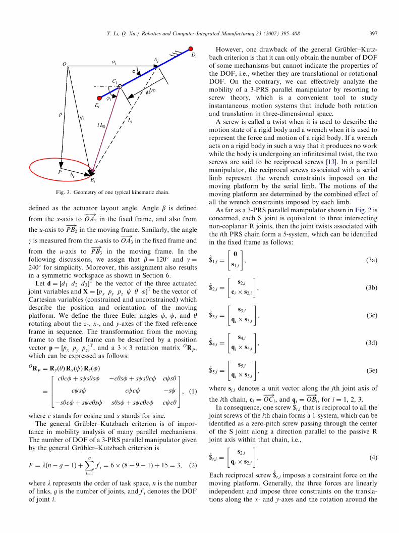
The vectors and reference frames are described in Figs. 2and 3. For the sake of analysis, as shown in Fig. 2, a fixedCartesian reference coordinate frame Ofx; y; zg is attachedat the centered point O of the fixed triangle base platformDA1A2A3. And a moving coordinate frame Pfu; v;wg isattached on the moving platform at point P which is thecentered point of triangle DB1B2B3. For simplicity andwithout losing the generality, let the x-axis point in thedirection of vector OA1

��!and the u-axis point along vector

PB1��!

.The three rails DiEi for i ¼ 1, 2, and 3 intersect each

other at the vertex N of the cone and intersect the x–y

plane at points A1, A2, and A3 that lie on a circle of radius

a. The three links CiBi for i ¼ 1, 2, and 3 with the lengthof l intersect the u–v plane at points B1, B2, and B3 whichlie on a circle of radius b. The sliders of the P joints arerestricted to move along the rails between Di and Ei. Anglea is measured from the fixed base to rails DiEi and is

ARTICLE IN PRESS

Fig. 3. Geometry of one typical kinematic chain.

Y. Li, Q. Xu / Robotics and Computer-Integrated Manufacturing 23 (2007) 395–408 397

defined as the actuator layout angle. Angle b is defined

from the x-axis to OA2

��!in the fixed frame, and also from

the u-axis to PB2��!

in the moving frame. Similarly, the angle

g is measured from the x-axis to OA3

��!in the fixed frame and

from the u-axis to PB3��!

in the moving frame. In thefollowing discussions, we assign that b ¼ 120� and g ¼240� for simplicity. Moreover, this assignment also resultsin a symmetric workspace as shown in Section 6.

Let d ¼ ½d1 d2 d3�T be the vector of the three actuated

joint variables and X ¼ ½px py pz c y f�T be the vector ofCartesian variables (constrained and unconstrained) whichdescribe the position and orientation of the movingplatform. We define the three Euler angles f, c, and yrotating about the z-, x-, and y-axes of the fixed referenceframe in sequence. The transformation from the movingframe to the fixed frame can be described by a positionvector p ¼ ½px py pz�

T, and a 3� 3 rotation matrix ORP,which can be expressed as follows:

ORP ¼ RyðyÞRxðcÞRzðfÞ

¼

cycfþ scsysf �cysfþ scsycf ccsy

ccsf cccf �sc

�sycfþ sccysf sysfþ sccycf cccy

2664

3775, ð1Þ

where c stands for cosine and s stands for sine.The general Grubler–Kutzbach criterion is of impor-

tance in mobility analysis of many parallel mechanisms.The number of DOF of a 3-PRS parallel manipulator givenby the general Grubler–Kutzbach criterion is

F ¼ lðn� g� 1Þ þXg

i¼1

f i ¼ 6� ð8� 9� 1Þ þ 15 ¼ 3, (2)

where l represents the order of task space, n is the numberof links, g is the number of joints, and f i denotes the DOFof joint i.

However, one drawback of the general Grubler–Kutz-bach criterion is that it can only obtain the number of DOFof some mechanisms but cannot indicate the properties ofthe DOF, i.e., whether they are translational or rotationalDOF. On the contrary, we can effectively analyze themobility of a 3-PRS parallel manipulator by resorting toscrew theory, which is a convenient tool to studyinstantaneous motion systems that include both rotationand translation in three-dimensional space.A screw is called a twist when it is used to describe the

motion state of a rigid body and a wrench when it is used torepresent the force and motion of a rigid body. If a wrenchacts on a rigid body in such a way that it produces no workwhile the body is undergoing an infinitesimal twist, the twoscrews are said to be reciprocal screws [13]. In a parallelmanipulator, the reciprocal screws associated with a seriallimb represent the wrench constraints imposed on themoving platform by the serial limb. The motions of themoving platform are determined by the combined effect ofall the wrench constraints imposed by each limb.As far as a 3-PRS parallel manipulator shown in Fig. 2 is

concerned, each S joint is equivalent to three intersectingnon-coplanar R joints, then the joint twists associated withthe ith PRS chain form a 5-system, which can be identifiedin the fixed frame as follows:

$1;i ¼0

s1;i

" #, (3a)

$2;i ¼s2;i

ci � s2;i

" #, (3b)

$3;i ¼s3;i

qi � s3;i

" #, (3c)

$4;i ¼s4;i

qi � s4;i

" #, (3d)

$5;i ¼s5;i

qi � s5;i

" #, (3e)

where sj;i denotes a unit vector along the jth joint axis of

the ith chain, ci ¼ OCi

��!, and qi ¼ OBi

��!, for i ¼ 1, 2, 3.

In consequence, one screw $r;i that is reciprocal to all thejoint screws of the ith chain forms a 1-system, which can beidentified as a zero-pitch screw passing through the centerof the S joint along a direction parallel to the passive Rjoint axis within that chain, i.e.,

$r;i ¼s2;i

qi � s2;i

" #. (4)

Each reciprocal screw $r;i imposes a constraint force on themoving platform. Generally, the three forces are linearlyindependent and impose three constraints on the transla-tions along the x- and y-axes and the rotation around the

ARTICLE IN PRESSY. Li, Q. Xu / Robotics and Computer-Integrated Manufacturing 23 (2007) 395–408398

z-axis, hence allow 3-DOF of the moving platform of a3-PRS parallel manipulator, which are rotations about thex- and y-axes, and a translational motion along the z-axis.A 3-PRS parallel manipulator has potential applica-tions where the orientation and reachable distance in z

direction are more important than the translations in x andy directions.

In addition, the mobility analysis of the 3-PRS parallelmanipulator can be implemented successfully by adoptinga recent theory of DOF for complex spatial mechanismsproposed in [14] as well.

3. Position kinematics analysis

3.1. Constraint conditions

The position vectors of points Ai and Bi with respect toframes O and P can be written as Oai and

Pbi, respectively,where a leading superscript indicates the coordinate framewith respect to which a vector is expressed. For brevity, theleading superscript will be omitted whenever the coordinateframe is the fixed frame, e.g., Oai ¼ ai. The vectors of ai

and Pbi can be expressed as follows, respectively:

a1 ¼ ½a 0 0�T, (5a)

a2 ¼ ½�a=2ffiffiffi3p

a=2 0�T, (5b)

a3 ¼ ½�a=2 �ffiffiffi3p

a=2 0�T, (5c)

Pb1 ¼ ½b 0 0�T, (6a)

Pb2 ¼ ½�b=2ffiffiffi3p

b=2 0�T, (6b)

Pb3 ¼ ½�b=2 �ffiffiffi3p

b=2 0�T. (6c)

Let u, v, and w be three unit vectors defined along the u-, v-,and w-axes of the moving frame P. Then the rotationmatrix can be expressed in terms of the direction cosines ofu, v, and w as

ORP ¼

ux vx wx

uy vy wy

uz vz wz

264

375. (7)

The position vector qi pointing from O to the ith S joint Bi

can be expressed by

qi ¼ pþ bi, (8)

where

bi ¼ORP

Pbi.

Substituting Eqs. (6) and (7) into Eq. (8) yields

q1 ¼

px þ bux

py þ buy

pz þ buz

264

375, (9a)

q2 ¼

px � bux=2þffiffiffi3p

bvx=2

py � buy=2þffiffiffi3p

bvy=2

pz � buz=2þffiffiffi3p

bvz=2

2664

3775, (9b)

q3 ¼

px � bux=2�ffiffiffi3p

bvx=2

py � buy=2�ffiffiffi3p

bvy=2

pz � buz=2�ffiffiffi3p

bvz=2

2664

3775. (9c)

Considering the mechanical constraints imposed by the Rjoint, the S joint Bi can only move in the plane defined bythe ith linear actuator and ith link CiBi. Therefore thefollowing three equations hold:

q1y ¼ 0, (10)

q2y ¼ �ffiffiffi3p

q2x, (11)

q3y ¼ffiffiffi3p

q3x. (12)

Substituting the components of qi from Eq. (9) into Eqs.(10)–(12) yields

py þ buy ¼ 0, (13)

py �12 buy þ

ffiffi3p

2 bvy ¼ �ffiffiffi3pðpx �

12 bux þ

ffiffi3p

2 bvxÞ, (14)

py �12

buy �ffiffi3p

2bvy ¼

ffiffiffi3pðpx �

12

bux �ffiffi3p

2bvxÞ. (15)

Taking 2�(13)–(14)–(15) yields

vx ¼ uy. (16)

Subtracting Eq. (14) from Eq. (15), we can obtain

px ¼b

2ðux � vyÞ. (17)

Hence, Eqs. (13), (16), and (17) impose three constraints onthe motion of the moving platform.

3.2. Jacobian matrix generation

Referring to Fig. 3, the vector loop for the ith link can bewritten as

pþ bi ¼ ai þ didi0 þ l li0, (18)

where li0 is the unit vector along CiBi

��!, di represents the

linear displacement of the ith actuator, and di0 is thecorresponding unit vector directing along DiEi

��!for i ¼ 1, 2,

and 3, which can be expressed as follows:

d10 ¼ ½�ca 0 � sa�T, (19a)

d20 ¼ ½ca=2 �ffiffiffi3p

ca=2 � sa�T, (19b)

d30 ¼ ½ca=2ffiffiffi3p

ca=2 � sa�T. (19c)

Differentiating both sides of Eq. (18) with respect to timeyields

tp þ xp � bi ¼ uidi0 þ lxi � li0, (20)

ARTICLE IN PRESSY. Li, Q. Xu / Robotics and Computer-Integrated Manufacturing 23 (2007) 395–408 399

where ‘‘�’’ denotes the cross product between vectors, tp

and xp represent the three-dimensional linear and angularvelocity of the moving platform, respectively, ui is thevelocity of the ith linear actuator, and xi represents thethree-dimensional angular velocity of link CiBi.

The passive variables xi can be eliminated by dot-multiplying both sides of Eq. (20) with li0, which gives

li0 � tp þ li0 � ðxp � biÞ ¼ uili0 � di0, (21)

where ‘‘�’’ denotes the dot product between vectors.Making use of formulae a � b ¼ b � a and a � ðb� cÞ ¼

b � ðc� aÞ ¼ c � ða� bÞ, Eq. (21) can be rewritten as

li0 � tp þ ðbi � li0Þ � xp ¼ uili0 � di0. (22)

Let _X ¼ ½tp xp�T and _d ¼ ½ _d1

_d2_d3�

T be the vectors of themoving platform velocities and the actuated joint rates,respectively. Then, Eq. (22) can be written in the matrixform:

Jx_X ¼ Jq

_d, (23)

where

Jx ¼

lT10 ðb1 � l10ÞT

lT20 ðb2 � l20ÞT

lT30 ðb3 � l30ÞT

264

3753�6

, (24)

Jq ¼

l10 � d10 0 0

0 l20 � d20 0

0 0 l30 � d30

264

3753�3

. (25)

When the manipulator is away from singularities, we have

_d ¼ Ja_X, (26)

where Ja ¼ J�1q Jx is a 3� 6 matrix. Eq. (26) represents theinverse velocity solution for a 3-PRS parallel manipulator.It should be noted that the six linear and angular velocitycomponents in _X are not all independent since a 3-PRSparallel manipulator possesses only 3-DOF. The relationsbetween the components of _X are expressed by thefollowing Eq. (32).

Substituting the components of u and v expressed inEq. (1) into the three constraint equations (13), (16), and(17) yields

py þ bccsf ¼ 0, (27)

�cysfþ scsycf ¼ ccsf, (28)

b

2ðcycfþ scsysf� cccfÞ ¼ px. (29)

Due to the physical constraints introduced by cone anglelimits of the S joints, the moving platform cannot rotateabout the x- and y-axes unlimitedly, i.e., �p=2oc; yop=2,then ccþ cya0. From Eq. (28), we can obtain

f ¼ Atan2ðscsy; ccþ cyÞ. (30)

Substituting f into Eqs. (27) and (29), respectively,allows the generation of px and py, which are expressed by

Eqs. (29) and (31), respectively:

py ¼ �bccsf. (31)

Let pz, c, and y be specified independent variables.Substitution of these three values into Eqs. (29)–(31)allows calculation of the constrained variables px, py, andf. Let _x ¼ ½ _pz

_c _y�T. When the manipulator is away fromsingularities, we have

_X ¼ Jr _x, (32)

where

Jr ¼

qpx

qpz

qpx

qcqpx

qyqpy

qpz

qpy

qc

qpy

qy1 0 0

0 1 0

0 0 1qfqpz

qfqc

qfqy

2666666666666664

3777777777777775. (33)

In view of Eqs. (26) and (32), we can get

_d ¼ J _x, (34)

where J ¼ JaJr is the 3� 3 Jacobian matrix which includesthe effect of the mechanical constraints on the mechanism,and is called the constrained Jacobian matrix of a 3-PRSparallel manipulator.

3.3. Inverse position kinematics modeling

The inverse position kinematics problem solves theactuated variables from a given position and orientationof the output platform.Referring to Fig. 3, we can obtain

Li ¼ didi0 þ l li0 (35)

and

Li ¼ qi � ai, (36)

where qi is expressed by Eq. (8) and Li is the vectorpointing from point Ai to Bi.In view of Eq. (35), we can get

Li � didi0 ¼ l li0. (37)

Squaring both sides of Eq. (37) and rearranging the itemsyield

d2i � 2diLi � di0 þ Li � Li � l2 ¼ 0. (38)

Solving Eq. (38) leads to the inverse position kinematicssolutions

di ¼ ðLi � di0Þ �

ffiffiffiffiffiffiffiffiffiffiffiffiffiffiffiffiffiffiffiffiffiffiffiffiffiffiffiffiffiffiffiffiffiffiffiffiffiffiffiffiffiffiffiffiffiffiðLi � di0Þ

2� Li � Li þ l2

q. (39)

We can see that there exist two solutions for each actuator,thus there are eight possible solutions for a given platform

ARTICLE IN PRESSY. Li, Q. Xu / Robotics and Computer-Integrated Manufacturing 23 (2007) 395–408400

position and orientation. To enhance the stiffness of themanipulator, only the negative square root is selected toyield a solution where the three legs are inclined inwardfrom top to bottom.

3.4. Forward position kinematics modeling

Given a set of actuated inputs, the position and orienta-tion of the output platform are solved by the forwardposition kinematics.

Let ji be measured from the fixed base to CiBi

��!as

represented in Fig. 3, then the three vectors q1, q2, and q3can be expressed as

q1 ¼

a� d1ca� lcj1

0

�d1sa� lsj1

264

375, (40a)

q2 ¼

�ða� d2ca� lcj2Þ=2ffiffiffi3pða� d2ca� lcj2Þ=2

�d2sa� lsj2

264

375, (40b)

q3 ¼

�ða� d3ca� lcj3Þ=2

�ffiffiffi3pða� d3ca� lcj3Þ=2

�d3sa� lsj3

264

375. (40c)

Considering the geometric distance between two S joints Bi

and Bj is equal to a constant, i.e., kBiBj

��!k ¼

ffiffiffi3p

b (iaj), thefollowing equations can be derived:

½qi � qiþ1�T½qi � qiþ1� � 3b2

¼ 0 ði ¼ 1; 2; 3Þ. (41)

Substituting Eq. (40) into Eq. (41) yields

e1icjicjiþ1 þ e2isjisjiþ1 þ e3icji þ e4isji

þ e5icjiþ1 þ e6isjiþ1 þ e7i ¼ 0, ð42Þ

where e1i ¼ l2, e2i ¼ �2l2, e3i ¼ ½ð2di þ diþ1Þca� 3a�l,e4i ¼ 2lðdi � diþ1Þsa, e5i ¼ ½ðdi þ 2diþ1Þca� 3a�l, e6i ¼ �2l

ðdi � diþ1Þsa, e7i ¼ ðdi � diþ1Þ2þ 3didiþ1c2a �3aðdiþ

2diþ1Þcaþ 3ða2 � b2Þ þ 2l2, for i ¼ 1, 2, and 3.

Substituting the trigonometric identities

sji ¼2ti

1þ t2iand cji ¼

1� t2i1þ t2i

ti ¼ tanji

2

� �into Eq. (42) yields three fourth-degree polynomials in t1,t2, and t3:

R1it2i t2iþ1 þR2itit

2iþ1 þR3it

2i tiþ1 þR4it

2i þR5it

2iþ1

þR6ititiþ1 þR7iti þR8itiþ1 þR9i ¼ 0, ð43Þ

where R1i ¼ e1i � e3i � e5i þ e7i, R2i ¼ 2e4i, R3i ¼ 2e6i,R4i ¼ �e1i � e3i þ e5i þ e7i, R5i ¼ �e1i þ e3i � e5i þ e7i,R6i ¼ 4e2i, R7i ¼ 2e4i, R8i ¼ 2e6i, R9i ¼ e1i þ e3i þ e5iþ

e7i, for i ¼ 1, 2, and 3.In what follows, the Sylvester dialytic elimination

method is applied to reduce the system of equations inEq. (43) to a 16th-degree polynomial in one variable.

Firstly, in order to eliminate t3, writing Eq. (43) for i ¼ 2and 3 yields two second-degree polynomials in t3:

At23 þ Bt3 þ C ¼ 0, (44)

Dt23 þ Et3 þ F ¼ 0, (45)

where A, B, and C are all second-degree polynomials in t2,and D, E, and F are second-degree polynomials in t1.Taking (45)�A–(44)�D and (45)�C–(44)�F , respec-

tively, and rewriting the two equations in matrix form weobtain

AE � BD AF � CD

CD� AF CE � BF

� �t3

1

� �¼

0

0

� �. (46)

Eq. (46) represents a system of two linear equations in t3and 1. The following equation can be obtained by equatingthe determinant of the coefficient matrix to zero:

ðAE � BDÞðCE � BF Þ þ ðAF � CDÞ2 ¼ 0. (47)

Secondly, for the purpose of eliminating t2, we writeEq. (47) in the form

Lt42 þMt32 þNt22 þ Pt2 þQ ¼ 0, (48)

where L, M, N, P, and Q are all fourth-degree polynomialsin t1.We also write Eq. (43) for i ¼ 1 in the form of

Gt22 þHt2 þ I ¼ 0, (49)

where G, H, and I are second-degree polynomials in t1.Now we can eliminate the unknown t2 from Eqs. (48)

and (49) as follows.Taking (49)�Lt2–(48)�G, we obtain

ðHL� GMÞt32 þ ðIL� GNÞt22 � GPt2 � GQ ¼ 0. (50)

Taking (49)�ðGt2 þHÞ–(48) �ðLt32 þMt22Þ yields

ðGN � LIÞt32 þ ðGPþHN �MIÞt22 þ ðGQþHPÞt2

þHQ ¼ 0. ð51Þ

Multiplying Eq. (49) by t2, we have

Gt32 þHt22 þ It2 ¼ 0. (52)

Eqs. (49)–(52) can be considered as four linear homo-geneous equations in the four variables of t32, t22, t2, and 1.The characteristic determinant is

HL� GM IL� GN �GP �GQ

GN � LI GPþHN �MI GQþHP HQ

G H I 0

0 G H I

26664

37775 ¼ 0.

(53)

Expanding Eq. (53) results in an eighth-degree polynomialin t21. It follows that there are at most eight pairs ofsolutions for t1, one being the negative of the other. Once t1is found, a unique value of t2 can be calculated by settingthe first-degree greatest common divisor between Eqs. (48)and (49) to be zero, and a unique value of t3 can then be

ARTICLE IN PRESS

Table 1

Results of using Newton iterative method to solve the forward position

kinematics problem

pz (mm) c (rad) y (rad)

0 �468 0.35 �0:251 �470:129683164667 0.400795016562 �0:2981554814582 �470:000294997604 0.399999621592 �0:2999976099673 �469:999988966593 0.400000066234 �0:3000001498384 �469:999988966119 0.400000066232 �0:300000149846

Y. Li, Q. Xu / Robotics and Computer-Integrated Manufacturing 23 (2007) 395–408 401

computed by solving Eq. (46). Consequently, there are atotal of 16 sets of solutions for j1, j2, and j3 [15].

The position vectors q1, q2, and q3 can be found bysubstituting the values of ji into Eq. (40). Then theposition vector of the moving platform is obtained as

p ¼ 13ðq1 þ q2 þ q3Þ. (54)

And the components of rotation matrix ORP can be foundby

u ¼q1 � p

b, (55)

v ¼q2 � q3ffiffiffi

3p

b, (56)

w ¼ u� v. (57)

Then the Euler angles c, y, and f can be solved as followsby considering Eqs. (1) and (7) together, i.e.,

c ¼ Atan2 �wy;ffiffiffiffiffiffiffiffiffiffiffiffiffiffiffiu2

y þ v2y

q� �, (58)

y ¼ Atan2ðwx;wzÞ, (59)

f ¼ Atan2ðuy; vyÞ. (60)

All possible configurations of the moving platform canbe derived through this approach; however, it is a verytime-consuming work and many solutions are meaning-less. Hence, we solve the forward position kinematicsproblem numerically by the classical Newton iterativemethod.

At a certain pose of a 3-PRS parallel manipulator, asystem of three equations can be written as

f ðpz;c; yÞ ¼ dðpz;c; yÞ � dgiven ¼ 0, (61)

where dðpz;c; yÞ is the joint space coordinates vectorgenerated from the inverse position kinematics solutionand dgiven is the known joint space coordinate vector whichcan be measured.

Let a given set of ðpnz ; cn; yn

Þ be denoted by xn. TheNewton iterative method is given by

xkþ1 ¼ xk �qf ðxkÞ

qx

� ��1f ðxkÞ. (62)

It can be shown that qf ðxkÞ=qx ¼ JðxkÞ, hence, Eq. (62) canbe written as

xkþ1 ¼ xk � JðxkÞ� �1

dðxkÞ � dgiven�

. (63)

Starting with an initial estimate x0, the iterative process willend once the maximum of the absolute value of ½dðxkÞ �

dgiven� is less than a specified tolerance.A computer program is developed to implement the

Newton iterative method. For the kinematic parameters ofa 3-PRS parallel manipulator; a ¼ 400mm, b ¼ 200mm,l ¼ 550mm, and a ¼ 30�, let the moving platform be in theCartesian pose

½pz c y�T ¼ ½�470 0:4 � 0:3�T. (64)

Then the constrained variables can be obtained fromEqs. (13), (16), and (17) as

½px py f�T ¼ ½4:1256 11:2767 � 0:0613�T, (65)

where the linear displacements are in unit of millimetersand the angular displacements are in unit of radians.The joint space coordinate vector can be derived from

the inverse position kinematics solutions as

½d1 d2 d3�T ¼ ½�101:4888 � 91:8057 80:5667�T, (66)

where all the actuated joint lengths are in unit of millimeters.We assume that dgiven is given by Eq. (66), which may be

measured from the joint space, and we need to find anapproximate numerical solution for x. Applying thenumerical technique presented above with an initial guess

x0 ¼ ð�468; 0:35; �0:25Þ, (67)

which deviates a little from the desired pose described byEq. (64), and choosing a specified tolerance 1E-6 as thestopping criterion, the convergence is reached after fouriterations as elaborated in Table 1.Regarding the selection of the initial guess, it is necessary

to select a set of values as close as possible to the actualpose of the moving platform since there are multipleforward kinematics solutions. In practice, such an initialguess could be chosen as the desired pose calculated fromthe analytical forward position kinematics analysis or themeasured pose of the moving platform at the initialconfiguration, or even the previous point on the trajectoryat a short time interval in the past.

4. Velocity kinematics analysis

4.1. Inverse velocity analysis

The objective of inverse velocity analysis of a 3-PRSparallel manipulator is to determine the required velocitiesof the three linear actuators from a given velocity of themoving platform in a given pose. The inverse velocitysolution of a 3-PRS parallel manipulator is expressed byEq. (26).

4.2. Forward velocity analysis

The objective of the forward velocity analysis for a 3-PRS parallel manipulator is to determine the velocity of the

ARTICLE IN PRESSY. Li, Q. Xu / Robotics and Computer-Integrated Manufacturing 23 (2007) 395–408402

moving platform from a given set of velocities of theactuators in a given pose.

Differentiating Eq. (8) with respect to time yields

tBi ¼ tp þ xp � bi, (68)

where tBi represents the three-dimensional velocity of theith S joint.

Let li0 represent a unit vector of the ith passive R jointaxis. Considering the mechanical constraints imposed by Rjoints again, we can see that tBi is perpendicular to li0.Then dot-multiplying both sides of Eq. (68) by li0 gives

0 ¼ li0 � tp þ li0 � ðxp � biÞ. (69)

Rearranging Eq. (69), we have

li0 � tp þ ðbi � li0Þ � xp ¼ 0. (70)

Writing Eq. (70) three times, and expressing them into thematrix form, yields

Jg_X ¼ 03�1, (71)

where

Jg ¼

lT10 ðb1 � l10Þ

T

lT20 ðb2 � l20Þ

T

lT30 ðb3 � l30Þ

T

264

3753�6

, (72)

and 03�1 denotes a 3� 1 zero matrix.Writing Eqs. (23) and (71) together yields

Jf_X ¼ Je

_d

03�1

" #, (73)

where

Jf ¼Jx

Jg

" #6�6

and Je ¼Jq 03�3

03�3 03�3

" #,

where 03�3 denotes a 3� 3 zero matrix.When Jf is invertible, Eq. (73) can be written as

_X ¼ Jb

_d

03�1

" #, (74)

where Jb ¼ J�1f Je. Eq. (74) represents the forward velocitysolution for a 3-PRS parallel manipulator.

5. Singularity analysis

The knowledge on the manipulator singularities isimportant both for singularity-free path planning and forthe geometric design of a desired manipulator workspacefree from singularities at the design stage of the manip-ulator. Numerous researchers have investigated singularityproblems of parallel manipulators because of theirnecessity to the design and control purposes [16–18].

Concerning a 3-PRS parallel manipulator, singularityanalysis is generally based on the instantaneous kinematics,which is described by Eq. (23):

Jx_X ¼ Jq

_d,

where _X and _d denote the vectors of output movingplatform velocities and input actuated joint rates, respec-tively.Based on the rank deficiency of matrices Jx and Jq, three

kinds of singularities can be identified [16]. The physicalmeaning of the three types of singularities for a 3-PRSparallel manipulator is discussed below.(1) The first kind of singularity, which is also called the

inverse kinematic singularity, occurs when Jq is notinvertible, i.e., detðJqÞ ¼ 0. From Eq. (25), we can see thisis the case when

li0 � di0 ¼ 0 ði ¼ 1; 2; 3Þ, (75)

i.e., the directions of one or more of the legs areperpendicular to their corresponding actuator directions.In this case, the manipulator loses one or more DOFdepending on the numbers of legs which are perpendicularto the corresponding actuator directions.(2) The second kind of singularity, which is also termed

as the direct kinematic singularity, will arise when Jx is notinvertible. Because the matrix Jx as expressed in Eq. (24) isnot a square matrix, the direct kinematic singularity occurswhen the matrix is not of full rank, i.e., its rank is equal to2 or 1. From Eq. (24), we can see that ni ¼ bi � li0 indeedrepresents a vector that is normal to the plane containingpoints P, Ci, and Bi, therefore the three vectors of ni are allparallel to the fixed base platform plane. But Jx is not rankdeficient even if ni are linearly dependent or only one of thethree vectors has zero components. If two or all of the threevectors have zero components, Jx becomes singular, i.e.,

bi � li0 ¼ 0 ði ¼ 1; 2; 3Þ. (76)

This condition implies that the links are aligned with themoving platform, with the extensions of lines CiBi passingthrough the center point P of the moving platform. In thiscase, the manipulator gains one or more DOF even whenall the actuators are locked.(3) The third kind of singularity, which is also termed as

the combined singularity, occurs when Jq is not invertibleand Jx is not of full rank. Generally, this type of singularitycan occur only for manipulators with special kinematicarchitectures. One example of this kind of singularity is

given in Fig. 4, where A1C1

���!? C1B1

���!, C2B2

���!and C3B3

���!are in

the plane of the moving platform and the extensions oflines C2B2 and C3B3 pass through point P. At suchconfiguration, the moving platform can undergo infinite-simal rotation about the line B2B3 while all the actuatorsare locked. And an infinitesimal motion of the linearactuator C1 causes no motion of the moving platform.Besides the three kinds of singularities, there exists still

another type of singularity for a 3-PRS parallel manip-ulator, which cannot be generated using the conventionalmethod of matrix analysis mentioned above, i.e., it cannotbe derived even when Jq and Jx are not of full rank, but canbe generated with the reciprocal screw theory [14]. Thistype of singularity can be called constraint singularity [18],which arises when the kinematic chains of a less DOF

ARTICLE IN PRESS

Fig. 4. The third kind of singularity for a 3-PRS parallel manipulator.

Fig. 5. A constraint singularity for a 3-PRS parallel manipulator.

Y. Li, Q. Xu / Robotics and Computer-Integrated Manufacturing 23 (2007) 395–408 403

parallel manipulator cannot constrain the moving platformto the planned motion any more.

Constraint singularities for a 3-PRS parallel manipulatoroccur when the three constraint forces, i.e., the threereciprocal screws $r;i, are linearly dependent, i.e., they lie ina common plane and intersect at one point, and thenimpose less than three constraints on the moving platform,thus the moving platform gains one or more DOF undersuch conditions.

Fig. 5 illustrates one such kind of singularity, where thethree zero-pitch reciprocal screws $r;1, $r;2, and $r;3 intersectat point B1, and impose only two constraints on themoving platform. The moving platform gains one moreDOF which rotates about the z-axis, and can instanta-neously move with 4-DOF. Therefore, it can rotatearbitrarily about point B1 and translate vertically. In suchconfigurations, since the three constraint forces arehorizontal, the moving platform and the base platformmust be parallel. Thus this type of singularity can occuronly when the moving platform is upside down as shown inFig. 5. Because of the physical constraints mainly imposedby the S joints, this type of singularity is unlikely to occurin practice, but such a detailed study can bring an insightinto the kinematics of a 3-PRS parallel manipulator.

6. Workspace analysis

In this section, we focus on studying the characteristicchanges in the reachable workspace of a 3-PRS parallelmanipulator if the actuator layout angle is varied. It is wellknown that compared with serial ones, parallel manip-ulators have relatively small workspace. Thus, the work-space of a parallel manipulator is one of the mostimportant aspects to reflect its working capacity, and it isnecessary to analyze the shape and volume of the work-space for enhancing the applications of parallel manip-ulators [17].

6.1. Algorithms

The reachable workspace of a parallel manipulator isdefined as the space that can be reached by the referencepoint with at least one orientation. We select the centroid Pof the moving platform as the reference point.By changing the coordinates of three P joints within their

motion ranges and resorting to solutions of the forwardposition kinematics, the workspace shape can be easilyexpressed in three-dimensional space by a series of dots.From the easily derived results, it is observed that thereexists no void within the workspace, i.e., the cross sectionof workspace is consecutive at every height. This allows usto divide the whole workspace of the manipulator into aseries of sub-workspace that are parallel to the baseplatform, then adopt a numerical search method todetermine the boundary of each sub-workspace, andcalculate the volume of the reachable workspace quantita-tively.As shown in Fig. 6, in a particular sub-workspace at the

height of Zi (within the workspace), to determine theboundary of the sub-workspace is to determine a series ofpoints in a polar vector ri

! which are farthest away fromthe z-axis as the polar vector ri

! rotates about the z-axisfrom 0 to 2p. When the boundary point in the direction ofri! is found as Piðricyz; risyz; ZiÞ, where ri is the distancebetween Zi and Pi, yz will be increased by Dyz, and the nextpoint will be found again. The determination of point Pi isbased on the inverse position kinematics solutions alongwith the consideration of the physical constraints discussedin what follows. Searching the next boundary point Piþ1,we can set the initial value of riþ1 as ri, and judge whetherpoint Piþ1 is within workspace; if yes, then increase riþ1, ifno, then decrease riþ1, until point Piþ1 lies on the boundaryof workspace. By this approach, the efficiency of searching

ARTICLE IN PRESS

Fig. 6. Determination of boundary points.

Fig. 7. Cone angle of the spherical joint.

Y. Li, Q. Xu / Robotics and Computer-Integrated Manufacturing 23 (2007) 395–408404

will be increased greatly. Once the boundary points in thesub-workspace are all searched out, Zi will be increased byDz, and the new searching will be performed again.

The workspace volume can also be calculated quantita-tively. As shown in Fig. 6, when yz is increased by Dyz, theunit volume of the corresponding workspace can beexpressed approximately as

dV ¼Dyz

2ppr2i Dz. (77)

Taking integral of Eq. (77) within the entire workspace, thevolume of the reachable workspace can be calculated by

V ¼XZmax

Zi¼Zmin

X2pyz¼0

1

2r2i Dyz Dz

�. (78)

6.2. Physical constraints

During the design of a practical manipulator, physicalconstraints should be considered in terms of the cone anglelimits of the S joints and the motion ranges of the linearactuators. Unlike the constraints imposed by the R jointsthat limit the effective DOF of the manipulator, thephysical constraints discussed here primarily limit theshape and size of the manipulator workspace. Since the Sjoints are not easy to manufacture, we mainly discuss theeffects imposed by the S joints.

Let the home position of a 3-PRS parallel manipulatorbe in the case of di ¼ 0 (i ¼ 1; 2; 3). As the socket of each Sjoint is rigidly attached to the moving platform, the axis ofsymmetry of each socket intersects the normal line of themoving platform at point M as described in Fig. 7, and thecone angle of the ith S joint can be expressed by the angle

between vectors CiBi

��!and BiM

��!as follows:

xi ¼ cos�1CiBi

��!� BiM��!

kCiBi

��!k kBiM��!k

!ði ¼ 1; 2; 3Þ. (79)

We assume that 0pxip45�, and the motion range of eachlinear actuator is within �150mm.

6.3. Case studies

The architectural parameters of a 3-PRS parallelmanipulator are selected as a ¼ 400mm, b ¼ 200mm,l ¼ 550mm, b ¼ 120�, and g ¼ 240�. The workspace ofthe manipulator is generated by a MATLAB program. Oneexample is shown in Fig. 8 when the actuator layout angleis a ¼ 30�.It is observed from Fig. 8 that the reachable workspace is

120�-symmetrical about the motion directions of threeactuators. In the upper and lower ranges of the workspace,the cross section has a triangular shape, while in the middlerange of the workspace, the cross-sectional shape is morelike a circle, which can be observed from the top view of thecontour plots as shown in Fig. 8(b).The simulation results of reachable workspace volume of

a 3-PRS parallel manipulator with the changing of theactuator layout angle are illustrated in Fig. 9, from which itcan be observed that the maximum workspace volumeoccurs when a is around 75�. The maximum range of thereachable workspace in the z-axis direction occurs when ais between 45� and 75� as shown in Fig. 10.

7. Dexterity analysis

The dexterity of a manipulator can be understood as theability of the manipulator to arbitrarily change its positionand orientation, or apply forces and torques in arbitrarydirections, and has emerged as a measure for manipulatorkinematic performance. The Jacobian matrix (along withits inverse and transpose) represents the mapping of both

ARTICLE IN PRESS

Fig. 8. Reachable workspace of a 3-PRS parallel manipulator: (a) three-

dimensional view; (b) x–y section at different heights.

Fig. 9. Reachable workspace volume versus actuator layout angle.

Y. Li, Q. Xu / Robotics and Computer-Integrated Manufacturing 23 (2007) 395–408 405

velocities and forces between the end-effector and theactuators of the manipulator, and thus any measure ofdexterity may be expressed in terms of properties of

Jacobian matrix. In this section, we are focused ondemonstrating the tendency of changes in dexteritycharacteristics of a 3-PRS parallel manipulator along withthe variance of actuator layout angle.

7.1. Dexterity indices

In related literatures, different indices of manipulatordexterity are introduced. One of the frequently used indicesis called kinematic manipulability that is proposed in [19]as the square root of the determinant of JJT. SinceJacobian (J) is configuration dependent, kinematic manip-ulability is a local performance measure, which also givesan indication of how close the manipulator is to thesingularity. For instance,

ffiffiffiffiffiffiffiffiffiffiffiffiffiffiffiffiffiffidetðJJTÞ

p¼ 0 means a singu-

larity configuration, and therefore we wish to maximize themanipulability index to avoid singularities. Anotherusually used index is the condition number of Jacobianmatrix recommended in [20]. As a measure of dexterity, thecondition number ranges in value from one (isotropy) toinfinity (singularity) and thus measures the degree of ill-conditioning of the Jacobian matrix, i.e., nearness of thesingularity. It is also local measure dependent solely on theconfiguration. A global dexterity index (GDI) is given in[21] as

GDI ¼

RVð1=kÞdV

V, (80)

where V is the total workspace volume and k denotes thecondition number of Jacobian and can be defined as

k ¼ kJk kJ�1k, (81)

where k � k denotes the 2-norm of the matrix.In the following discussions, we study the dexterity

characteristics of a 3-PRS parallel manipulator based onkinematic manipulability measure and global dexterityindex, respectively.

7.2. Case studies

The architectural parameters of a 3-PRS parallelmanipulator are selected as follows: a ¼ 400mm,b ¼ 200mm, l ¼ 550mm, b ¼ 120�, and g ¼ 240�. Assumethat the motion ranges of linear actuators are within�150mm, and the cone angle limits of the S joints are0pxip45�.

7.2.1. Kinematic manipulability

The manipulability ellipsoid is an intuitive and usefulmeasure to analyze a manipulator’s manipulability, whichcan be made by mapping a unit sphere in the input jointspace to the output task space through the Jacobianmatrix. From this physical insight, the manipulability of amanipulator was defined as follows [19]:

o ¼ffiffiffiffiffiffiffiffiffiffiffiffiffiffiffiffiffiffidetðJJTÞ

q. (82)

ARTICLE IN PRESS

Fig. 10. Reachable workspace range in the z-axis direction.

Fig. 11. Kinematic manipulability at a height of pz ¼ �460mm in case of

a ¼ 60�.

Fig. 12. Manipulability versus actuator layout angle at a height of

pz ¼ �460mm.

Y. Li, Q. Xu / Robotics and Computer-Integrated Manufacturing 23 (2007) 395–408406

As for a 3-PRS parallel manipulator presented here, inorder to have an intuitive view of this point, we explore themapping from input joint velocity space to output taskvelocity space through the Jacobian matrix. The unitsphere in joint space defined by _d

T _dp1 will be mapped intoan ellipsoid in task space expressed by _xTðJJTÞ _xp1, whichis known as velocity or kinematics or manipulabilityellipsoid. Along the directions of the major and minoraxes of the ellipsoid, the end-effector can move at large andsmall velocities, respectively. Furthermore, if the ellipsoidis larger and closer to a sphere, then the end-effector canmove fast and isotropically along all directions in the taskspace with a higher dexterity. Since a 3-PRS parallelmanipulator is nonredundant, manipulability measure o,which is proportional to the volume of the ellipsoid,reduces to

o ¼ jdetðJÞj. (83)

With the changing of actuator layout angle, we cancalculate the kinematics manipulability of a 3-PRS parallelmanipulator at every point within the workspace. Oneexample is shown in Fig. 11 in case of a ¼ 60� at a height ofpz ¼ �460mm, from which we can see that in the plane ata certain height, manipulability is maximal when the centerpoint of moving platform lies in the z-axis, and decreaseswhen the manipulator tends to the workspace boundary.

The minimal and maximal values of manipulabilityversus actuator layout angle changing from 0� to 120� areillustrated in Fig. 12. It is observed from Fig. 10 that theworkspace range in the z-axis direction is relatively limitedin case of a ¼ 0�, which is reflected in the height selected forthe comparison study of the manipulability at variousactuator layout angles.

From Fig. 12 we can see that the minimum of both theminimal and maximal values of manipulability occurswhen a is between 45� and 75�. That is, around 60�, themanipulability of a 3-PRS parallel manipulator is lowercompared with other actuator layout angles.

7.2.2. Global dexterity index

The global dexterity index (GDI) represents the unifor-mity of dexterity over the entire workspace other than thedexterity at certain configurations, and possesses severalfavorable characteristics. For example, it is normalized bythe workspace size and therefore gives a measure ofkinematic performance independent of the differing work-space volume of design candidates. Furthermore, thereciprocal of condition number is bounded between 0 and1, and is more convenient to handle than k, which tends toinfinity at singularities; hence, during numerical integra-tion, the number of sample points near singularities has areduced impact on the result since 1=k approaches zero atthose points. Because there exists no closed-form solutionfor GDI expressed by Eq. (80), the integral of the dexteritymust be calculated numerically, which can be approximated

ARTICLE IN PRESS

Fig. 14. Global dexterity index versus actuator layout angle.

Y. Li, Q. Xu / Robotics and Computer-Integrated Manufacturing 23 (2007) 395–408 407

by a discrete sum:

GDI 1

Nw

Xw2V

1

k, (84)

where w is one of Nw points which are uniformly distributedover the entire workspace of the manipulator.

As pointed out in [22,23], a problem remains for thecondition number as far as units are concerned whenJacobian matrix is dimensionally inhomogeneous. Obser-ving the matrix Jx in Eq. (24), we can see that the first threecolumns are dimensionless while the last three columnshave units of length. In order to homogenize the Jacobianmatrix, the last three columns can be divided by the radiusof the moving platform [24], i.e., Jxh ¼ Jx diagð1 1 1 1

b1b

1bÞ.

When the manipulator is away from singularities, Eq. (34)can be expressed as

_d ¼ Jh _x, (85)

where Jh ¼ J�1q JxhJr is the homogeneous Jacobian matrixof a 3-PRS parallel manipulator.

Then the condition number of Jacobian matrix can beexpressed as

k ¼ kJhk kJ�1h k. (86)

Fig. 13 depicts the grid map of the reciprocal of Jacobianmatrix condition number of a 3-PRS parallel manipulatorin case of a ¼ 60�, which shows the same tendency ofchanges as that described in Fig. 11. With the changing ofactuator layout angle, we can calculate the GDI of themanipulator over the entire workspace. And the simulationresults are represented in Fig. 14.

It is observed from Fig. 14 that the maximal GDI overthe entire workspace of a 3-PRS parallel manipulatoroccurs when a ¼ 120�, and decreases along with thedecreasing of actuator layout angle. But in the case ofa ¼ 120�, it is also observed from Fig. 9 that the workspacevolume is relatively small. Since the selection of manip-ulators depends heavily on the tasks to be performed,different objectives should be taken into account when the

Fig. 13. Reciprocal of condition number of Jacobian matrix at a height of

pz ¼ �460mm in case of a ¼ 60�.

actuator layout angle of a 3-PRS parallel manipulator isdesigned, or alternatively, several required performanceindices may be considered simultaneously.For example, a 3-PRS parallel kinematic machine tool or

a micro-motion manipulator with a compact structure canbe built with actuator layout angle a ¼ 90�, and a 3-PRSflight simulator with optimal dexterity performance can bedeveloped as a ¼ 120�. Moreover, as illustrated in Fig. 15,a medical 3-PRS parallel robot used for chest compressionsin the process of cardiopulmonary resuscitation (CPR) canbe established with a ¼ 75� so as to achieve an equalcompromise between the performances of GDI and spaceutility ratio which is defined as the ratio of total workspacevolume to physical size of the manipulator [25].

8. Conclusions

A systematic kinematics and kinematic characteristicanalysis of the 3-PRS parallel manipulator in considera-tions of the selection of the actuator layout angle fordifferent specific tasks is presented in this paper.Firstly, the mobility of the manipulator is analyzed

based on the reciprocal screw theory. Then, the inverseposition kinematics solution is derived in closed-form, theforward position kinematics problem is solved throughNewton iterative method, the velocity kinematics analysisis performed, and the singularity configurations includingthree kinds of conventional singularities and the constraintsingularity are derived. Taking into account the physicalconstraints introduced by cone angle limits of sphericaljoints and motion ranges of linear actuators, the reachableworkspace of the manipulator is generated via a numericalsearch method, and the workspace volume is calculatedand compared at various actuator layout angles. Thesimulation results show that the maximal reachable work-space of a 3-PRS parallel manipulator occurs around 75�

of the actuator layout angle. With the variations onactuator layout angle, the dexterity characteristics of the

ARTICLE IN PRESS

Fig. 15. A medical 3-PRS parallel manipulator for CPR.

Y. Li, Q. Xu / Robotics and Computer-Integrated Manufacturing 23 (2007) 395–408408

manipulator are investigated in detail based on a localsense measure—kinematic manipulability—and on a globalsense measure—global dexterity index—respectively. Thesimulation results illustrate that different objectives shouldbe considered when the actuator layout angle of a 3-PRSparallel manipulator is designed. The derived results arehelpful in designing suitable actuator layout angles of a 3-PRS parallel manipulator according to different objectives.

In future work, other characteristics of a 3-PRS parallelmanipulator with the changing of actuator layout anglewill be analyzed and compared, and the design parametersexcluding actuator layout angle will also be considered toachieve the required optimal output characteristics.

Acknowledgments

The authors appreciate the fund support from the researchcommittee of University of Macau under Grant No. RG083/04-05S/LYM/FST and Macao Science and TechnologyDevelopment Fund under Grant no. 069/2005/A.

References

[1] Merlet J-P. Parallel robots. London: Kluwer Academic Publishers;

2000.

[2] Clavel R. DELTA, a fast robot with parallel geometry. Proceedings

of 18th international symposium on industrial robots, Lausanne;

1988. p. 91–100.

[3] Tsai LW, Walsh GC, Stamper RE. Kinematics of a novel three DOF

translational platform. Proceedings of IEEE international conference on

robotics and automation, Minneapolis, Minnesota; 1996. p. 3446–51.

[4] Miller K, Synthesis of a manipulator of the new UWA robot.

Proceedings of Australian conference on robotics and automation,

Brisbane; 1999. p. 228–33.

[5] Gregorio RDi, Parenti-Castelli V. A translational 3-DOF parallel

manipulator. In: Lenarcic J, Husty ML, editors. Advances in robot

kinematics: analysis and control. Dordrecht: Kluwer Academic

Publishers; 1998. p. 49–58.

[6] Li Y, Xu Q. Kinematic analysis and design of a new 3-DOF

translational parallel manipulator. ASME J Mech Des 2006; in press.

[7] Ottaviano E, Gosselin CM, Ceccarelli M, Singularity analysis of

CaPaMan: a three-degree of freedom spatial parallel manipulator.

Proceedings of IEEE international conference robotics and automa-

tion, Seoul, Korea; 2001, p. 1295–300.

[8] Liu X-J, Tang X, Wang J. HANA: a novel spatial parallel

manipulator with one rotational and two translational degrees of

freedom. Robotica 2005;23(2):257–70.

[9] Lee KM, Arjunan S. A three-degrees-of-freedom micromotion in-

parallel actuated manipulator. IEEE Trans Robot Automat 1991;

7(5):634–41.

[10] Liu D, Che R, Li Z, Luo X. Research on the theory and the virtual

prototype of 3-DOF parallel-link coordinating-measuring machine.

IEEE Trans Instrum Meas 2003;52(1):119–25.

[11] Carretero JA, Podhorodeski RP, Nahon MA, Gosselin CM.

Kinematic analysis and optimization of a new three degree-of-

freedom spatial parallel manipulator. ASME J Mech Des 2000;

122(1):17–24.

[12] Tsai M-S, Shiau T-N, Tsai Y-J, Chang T-H. Direct kinematic

analysis of a 3-PRS parallel mechanism. Mech Mach Theory 2003;

38(1):71–83.

[13] Tsai LW. Robots analysis: the mechanics of serial and parallel

manipulator. New York: Wiley; 1999.

[14] Zhao J-S, Zhou K, Feng Z-J. A theory of degrees of freedom for

mechanisms. Mech Mach Theory 2004;39(6):621–43.

[15] Angeles J. Fundamentals of robotic mechanical systems. New York:

Springer; 2002.

[16] Gosselin CM, Angeles J. Singularity analysis of closed-loop

kinematic chains. IEEE Trans Robot Automat 1990;6(3):281–90.

[17] Li Y, Xu Q. Kinematics and dexterity analysis for a novel 3-DOF

translational parallel manipulator. Proceedings of IEEE international

conference on robotics and automation, Barcelona, Spain; 2005.

p. 2955–60

[18] Zlatanov D, Bonev IA, Gosselin CM. Constraint singularities of

parallel mechanisms. Proceedings of IEEE international conference

robotics and automation, Washington, DC; 2002. p. 496–502.

[19] Yoshikawa T. Manipulability of robotic mechanisms. Int J Robotics

Res 1985;4(2):3–9.

[20] Salisbury J, Craig J. Articulated hands: force control and kinematic

issues. Int J Robotics Res 1982;1(1):4–17.

[21] Gosselin C, Angeles J. A global performance index for the kinematic

optimization of robotic manipulators. ASME J Mech Des 1991;

113(3):220–6.

[22] Lipkin H, Duffy J. Hybrid twist and wrench control of a robotic

manipulator. ASME J Mech Transm Automat Des 1988;10(2):

138–44.

[23] Angeles J, Lopez-Cajun CS. Kinematic isotropy and the conditioning

index of serial robotic manipulators. Int J Robotics Res 1992;11(6):

560–71.

[24] Stoughton RS, Arai T. A modified Stewart platform manipulator

with improved dexterity. IEEE Trans Robot Automat 1993;9(2):

166–73.

[25] Li Y, Xu Q. Kinematic design and dynamic analysis of a medical

parallel manipulator for chest compression task. Proceedings of IEEE

international conference on robotics and biomimetics, Hong Kong

SAR and Macau SAR; 2005. p. 693–8.