
KATS Travel Model Update - Kalamazoo Area Transportation Study
183
June 29, 2015 www.camsys.com KATS Travel Model Update Technical Documentation prepared for Kalamazoo Area Transportation Study prepared by Cambridge Systematics, Inc. with Dunbar Transportation Consulting technical report
Transcript of KATS Travel Model Update - Kalamazoo Area Transportation Study
June 29, 2015 www.camsys.com
KATS Travel Model Update
Technical Documentation
prepared for
Kalamazoo Area Transportation Study
prepared by
Cambridge Systematics, Inc.
with
Dunbar Transportation Consulting
technical
report


report
KATS Travel Model Update
Technical Documentation
prepared for
Kalamazoo Area Transportation Study
prepared by
Cambridge Systematics, Inc. 999 18th Street, Suite 3000 Denver, CO 80202
with
Dunbar Transportation Consulting
date
June 29, 2015


KATS Travel Model Update
Cambridge Systematics, Inc. i 140078
Table of Contents
Introduction ..................................................................................................................... 1
1.0 Roadway Network .............................................................................................. 1-1
1.1 Roadway Network Development ............................................................. 1-1
Michigan Geographic Framework ........................................................... 1-1
Direction of Flow .................................................................................... 1-2
Grade Separation.................................................................................... 1-2
MGF Attribute Retention ...................................................................... 1-2
Speed Limit and Number of Lanes .......................................................... 1-4
Centroids and Centroid Connectors ........................................................ 1-4
Centroid Placement ............................................................................... 1-4
Centroid Connector Placement ............................................................ 1-5
Segment Consolidation .............................................................................. 1-6
Traffic Counts .............................................................................................. 1-7
1.2 Roadway Network Structure .................................................................... 1-8
Turn Penalties.............................................................................................. 1-8
Input and Output Networks ..................................................................... 1-8
Multi-Year and Alternative Network Structure ................................... 1-10
Representation of Networks by Year ................................................ 1-10
Representation of New Facilities ....................................................... 1-11
Representation of Network Alternatives .......................................... 1-11
Network Attribute Selection............................................................... 1-12
Network Attribute List ............................................................................ 1-15
Facility Type ......................................................................................... 1-17
Area Type .............................................................................................. 1-22
Link Speeds ............................................................................................. 1-2
Speed Feedback ...................................................................................... 1-4
Link Capacities ....................................................................................... 1-4
2.0 Transit Networks ................................................................................................ 2-1
2.1 Transit Route System ................................................................................. 2-3
Route System Attributes ............................................................................ 2-3
Route Headways .................................................................................... 2-3
Transit Stops ........................................................................................... 2-4

Table of Contents, continued
ii Cambridge Systematics, Inc. 140078
2.2 Transit Line Layer ....................................................................................... 2-5
Transit Travel Time .................................................................................... 2-5
Walk Access and Egress ............................................................................. 2-6
Timed Transfers .......................................................................................... 2-7
Drive Access ................................................................................................ 2-8
2.3 Transit Pathbuilding................................................................................... 2-8
3.0 Traffic Analysis Zones ....................................................................................... 3-1
3.1 Traffic Analysis Zone Structure ................................................................ 3-1
3.2 Household and Population Data .............................................................. 3-6
3.3 Employment and Enrollment Data ........................................................ 3-11
4.0 External Travel .................................................................................................... 4-1
4.1 External Station Volumes .......................................................................... 4-1
External-Internal Trips ............................................................................... 4-2
External-External Trips .............................................................................. 4-4
4.2 External Station Forecasts .......................................................................... 4-6
5.0 Household Survey Processing .......................................................................... 5-7
5.1 Survey Weighting and Expansion ............................................................ 5-7
Comparison to Observed Distributions .................................................. 5-8
Expansion Factor Development ................................................................ 5-9
Use of Additional Records ...................................................................... 5-11
5.2 Trip Purposes ............................................................................................ 5-12
5.3 TAZ Identification .................................................................................... 5-14
6.0 Trip Generation ................................................................................................... 6-1
6.1 Trip Productions ......................................................................................... 6-1
Income Group Definitions ......................................................................... 6-1
Cross Classified Production Rates............................................................ 6-2
6.2 Trip Attractions ........................................................................................... 6-5
Attraction Variables.................................................................................... 6-5
Classified Attraction Rates ........................................................................ 6-6
6.3 Non Home Based Production Allocation ................................................ 6-7
6.4 School and University Trips ...................................................................... 6-8
K-12 School Trips ........................................................................................ 6-8
HBSc Production Rates.......................................................................... 6-8
HBSc Attraction Rates ........................................................................... 6-9
University Trips .......................................................................................... 6-9

KATS Travel Model Update
Cambridge Systematics, Inc. iii 140078
University Definitions ........................................................................... 6-9
Trip Types at Universities ................................................................... 6-10
Employment and Enrollment Data ................................................... 6-11
Special Generator Values .................................................................... 6-12
University Production Allocation .......................................................... 6-13
6.5 Trip Rate Factors ....................................................................................... 6-15
6.6 Trip Balancing ........................................................................................... 6-15
6.7 Disaggregation Models ............................................................................ 6-16
Household Size Disaggregation Model ................................................. 6-16
Household Worker Disaggregation Model ........................................... 6-17
Household Income Disaggregation Model ........................................... 6-18
TAZ-Level Bivariate Data ........................................................................ 6-19
7.0 Trip Distribution ................................................................................................ 7-1
7.1 Peak and Off-Peak Period Definitions ..................................................... 7-2
7.2 Roadway Network Shortest Path ............................................................. 7-2
Terminal Times ........................................................................................... 7-3
Intrazonal Impedance ................................................................................ 7-3
7.3 Friction Factors ............................................................................................ 7-3
8.0 Mode Choice ........................................................................................................ 8-1
8.1 Observed Mode Shares .............................................................................. 8-1
8.2 Mode Choice Model Structure .................................................................. 8-2
Logit Model Background ........................................................................... 8-2
KATS Mode Choice Model Definition ..................................................... 8-5
Utility Functions ..................................................................................... 8-6
8.3 Auto Occupancy ......................................................................................... 8-9
9.0 Time of Day, Assignment, and Speed Feedback ........................................ 9-10
9.1 Time of Day ............................................................................................... 9-10
9.2 Traffic Assignment ................................................................................... 9-13
Closure Criteria ......................................................................................... 9-14
Impedance Calculations ........................................................................... 9-14
Volume-Delay Functions ......................................................................... 9-15
9.3 Speed Feedback ......................................................................................... 9-16
The Method of Successive Averages ...................................................... 9-16
Initial Speeds and Borrowed Feedback Results ................................... 9-17
Convergence Criteria ............................................................................... 9-18
Shortest path Root Mean Square Error ............................................. 9-18

Table of Contents, continued
iv Cambridge Systematics, Inc. 140078
Application of Speed Feedback for Alternatives Analysis ................. 9-18
9.4 Transit Assignment .................................................................................. 9-19
10.0 Model Validation ............................................................................................ 10-20
10.1 Traffic Assignment Validation .............................................................. 10-20
Overall Activity Level ............................................................................ 10-20
Screenlines ............................................................................................... 10-21
Measures of Error ................................................................................... 10-24
10.2 Transit Assignment Validation ............................................................. 10-25
Systemwide Transit Assignment Validation ...................................... 10-25
Route Group Validation ........................................................................ 10-26
10.3 Sensitivity Tests....................................................................................... 10-28
Socioeconomic Data Adjustments ........................................................ 10-28
Isolated Changes ................................................................................ 10-29
Wholesale Changes ............................................................................ 10-30
Link Removal .......................................................................................... 10-31
A. KMetro Schedules from 2010 ............................................................................... 1
B. Survey / Employment Correspondence ............................................................. 1

KATS Travel Model Update
Cambridge Systematics, Inc. v 140078
List of Tables
Table 1.1 Attributes Retained from the MGF ........................................................ 1-3
Table 1.2 Attributes preventing node removal ..................................................... 1-7
Table 1.3 Input Network Link fields .................................................................... 1-15
Table 1.4 Input Network Node fields .................................................................. 1-16
Table 1.5 Facility Types .......................................................................................... 1-18
Table 1.6 Area Types and Density Definitions ................................................... 1-23
Table 1.7 Speed Limit to Freeflow Speed Factors ................................................. 1-3
Table 1.8 Average Existing Speed Limit Values ................................................... 1-3
Table 1.9 Default Free Flow Speed Values ............................................................ 1-4
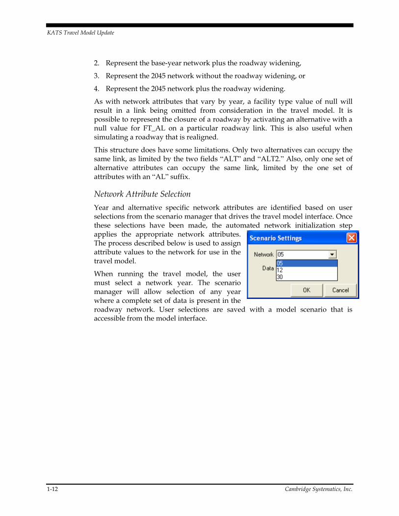
Table 1.10 Hourly Link Capacities (Upper limit LOS E) ....................................... 1-5
Table 2.1 Route Attributes ....................................................................................... 2-3
Table 2.2 Route Headway Assumptions ............................................................... 2-4
Table 2.3 Transit Stops Attributes .......................................................................... 2-5
Table 2.4 Key Fields in the Transit Line Layer ..................................................... 2-6
Table 2.5 Transit Path Building Weights ............................................................... 2-9
Table 3.1 TAZ Numbering Ranges ......................................................................... 3-2
Table 3.2 Population and Household Totals ......................................................... 3-7
Table 3.3 Hospital Employment Totals ................................................................ 3-11
Table 3.4 NAICS Code to Employment Type Correspondence ....................... 3-13
Table 3.5 2010 and 2045 Employment Data ........................................................ 3-14
Table 4.1 External Station Volumes and IE/EE Splits ......................................... 4-1
Table 4.2 External Trip Share and Auto Occupancy by Purpose ....................... 4-3
Table 4.3 Resulting IE/EI and EE trip totals for 2010 and 2045 ......................... 4-3
Table 4.4 External Trip Seed Matrix ....................................................................... 4-5
Table 4.5 External Trip Table .................................................................................. 4-5
Table 5.1 Survey and ACS Comparison: Household Income ............................ 5-8
Table 5.2 Survey and Census Comparison: Household Size ............................. 5-9

List of Tables, continued
vi Cambridge Systematics, Inc. 140078
Table 5.3 Survey and ACS Comparison: Household Vehicles ........................... 5-9
Table 5.4 Survey and ACS Comparison: Household Workers ........................... 5-9
Table 5.5 Expansion Summary: Household Income ......................................... 5-10
Table 5.6 Expansion Summary: Household Size ............................................... 5-10
Table 5.7 Expansion Summary: Household Vehicles ........................................ 5-10
Table 5.8 Expansion Summary: Household Workers ........................................ 5-11
Table 5.9 Trip Purpose Identification ................................................................... 5-13
Table 5.10 Number of Trips by Purpose ................................................................ 5-13
Table 6.1 Trip Rates by Income Range ................................................................... 6-2
Table 6.2 HBW Trip Production Rates ................................................................... 6-3
Table 6.3 HBS Trip Production Rates ..................................................................... 6-3
Table 6.4 HBO Trip Production Rates .................................................................... 6-4
Table 6.5 WBO Trip Production Rates ................................................................... 6-4
Table 6.6 OBO Trip Production Rates .................................................................... 6-4
Table 6.7 Trip Production Rate Summary ............................................................. 6-4
Table 6.8 NAICS Code to Employment Type Correspondence ......................... 6-6
Table 6.9 Trips by Attraction Rate Variable .......................................................... 6-7
Table 6.10 Trip Attraction Rates .............................................................................. 6-7
Table 6.11 WBO Production Allocation Rates ....................................................... 6-8
Table 6.12 HBSc Production Rates by Number of Children ................................ 6-9
Table 6.13 University Employment ........................................................................ 6-11
Table 6.14 University Enrollment ........................................................................... 6-11
Table 6.15 University Special Generator Values .................................................. 6-12
Table 6.16 Allocation of Special Generators to WMU Zones .............................. 6-13
Table 6.17 Trip Rate Factors .................................................................................... 6-15
Table 6.18 Income Group Definitions ................................................................... 6-19
Table 6.19 Bivariate Household Distribution, Household Size ......................... 6-20
Table 6.20 Bivariate Household Distribution, Household Workers ................. 6-20
Table 7.1 Peak and Off-Peak Trip Percentages by Purpose ................................ 7-2
Table 7.2 Terminal Times by Area Type ................................................................... 7-3

KATS Travel Model Update
Cambridge Systematics, Inc. vii 140078
Table 7.3 Coincidence Ratios and Average Trip Lengths ................................... 7-4
Table 7.4 Calibrated Friction Factor Parameters .................................................. 7-9
Table 8.1 Mode Share Targets ................................................................................. 8-2
Table 8.2 Utility Specifications ................................................................................ 8-7
Table 8.3 Utility Variable Coefficients ................................................................... 8-7
Table 8.4 FTA Mode Choice Model Coefficient Guidelines ............................... 8-8
Table 8.5 Alternative Specific Constants ............................................................... 8-8
Table 8.6 Average Auto Occupancy by Trip Purpose ......................................... 8-9
Table 9.1 Peak Period Definitions ......................................................................... 9-11
Table 9.2 Time of Day Factors ............................................................................... 9-13
Table 9.3 Peak and Off-Peak Trip Percentages by Purpose .............................. 9-13
Table 9.4 Traffic Assignment Time of Day Factors ............................................ 9-13
Table 9.5 Volume Delay Parameters Alpha and Beta ........................................ 9-15
Table 10.1 Regional Activity Validation .............................................................. 10-21
Table 10.2 Screenline Volumes and Counts ........................................................ 10-22
Table 10.3 Root Mean Square Error by Facility Type and Area Type ............. 10-25
Table 10.4 Root Mean Square Error by Volume Group ..................................... 10-25
Table 10.5 Systemwide Transit Validation Results ............................................ 10-26
Table 10.6 Route Group Definitions ..................................................................... 10-26
Table 10.7 TAZ Based Sensitivity Tests ............................................................... 10-30
Table 10.8 Base Year Sensitivity Test Household Data ..................................... 10-30
Table 10.9 Forecast Year Sensitivity Test Results ............................................... 10-31
Table 10.10 Network Change Sensitivity Test Results ........................................ 10-31


KATS Travel Model Update
Cambridge Systematics, Inc. ix 140078
List of Figures
Figure 1.1 Travel Model Folder Structure ............................................................. 1-10
Figure 1.2 Facility Type............................................................................................ 1-19
Figure 1.3 Facility Type (Urban area detail) ......................................................... 1-20
Figure 1.4 Area Type ................................................................................................ 1-25
Figure 1.5 Area Type (Urban Area Detail) .............................................................. 1-1
Figure 2.1 Connections between the Route System and Transit Line Layer ...... 2-1
Figure 2.2 Roadway and Transit Line Layer Processing ....................................... 2-2
Figure 2.3 Example Walk Access Paths ................................................................... 2-7
Figure 3.1 Traffic Analysis Zones ............................................................................. 3-5
Figure 3.2 Traffic Analysis Zones (urban area detail) ........................................... 3-6
Figure 3.3 Household Density (2010) ....................................................................... 3-9
Figure 3.4 Household Density (2045) ..................................................................... 3-10
Figure 3.5 Employment Density (2010) ................................................................. 3-15
Figure 3.6 Employment Density (2045) ................................................................. 3-16
Figure 4.1 External Station Locations ...................................................................... 4-1
Figure 5.1 Number of survey records by normalized weight ............................ 5-11
Figure 6.1 WMU and Kalamazoo College Traffic Analysis Zones .................... 6-10
Figure 6.2 Home Base University Production Allocation ................................... 6-14
Figure 6.3: Household Size Disaggregation Model ................................................ 6-17
Figure 6.4 Household Worker Disaggregation Model ........................................ 6-18
Figure 6.5: Household Income Disaggregation Model .......................................... 6-19
Figure 7.1 HBW Trip Length Frequency Distribution ........................................... 7-5
Figure 7.2 HBS Trip Length Frequency Distribution............................................. 7-6
Figure 7.3 HBSc Trip Length Frequency Distribution ........................................... 7-6
Figure 7.4 HBO Trip Length Frequency Distribution ........................................... 7-7
Figure 7.5 WBO Trip Length Frequency Distribution ........................................... 7-7
Figure 7.6 OBO Trip Length Frequency Distribution ............................................ 7-8

List of Figures, continued
x Cambridge Systematics, Inc. 140078
Figure 7.7 Calibrated Friction Factors...................................................................... 7-8
Figure 8.1 Example Multinomial Logit Structure .................................................. 8-3
Figure 8.2 Example Nested Logit Model ................................................................. 8-5
Figure 8.3 KATS Model Choice Model Structure ................................................... 8-6
Figure 9.1 Trip Share by Half Hour ....................................................................... 9-11
Figure 9.2 Approximate VMT Share by Half Hour ............................................. 9-12
Figure 10.1 Screenline Analysis .............................................................................. 10-22
Figure 10.2 Screenlines ............................................................................................. 10-23
Figure 10.3 Count / Volume Comparison ............................................................ 10-24
Figure 10.4 Kalamazoo Transit Route Groups ..................................................... 10-27
Figure 10.5 Transit Assignment Validation by Route Group ............................. 10-28
Figure 10.6 Sensitivity Test Zones .......................................................................... 10-29
Figure 10.7 Removal of an Urban Link .................................................................. 10-32
Figure 10.8 Removal of a Lightly Traveled Rural Link ....................................... 10-33

KATS Travel Model Update
Cambridge Systematics, Inc.
i-1
Introduction
The Kalamazoo Area Transportation Study and member jurisdictions use the KATS Regional Travel Model (KATS Model) as a tool to forecast traffic and travel in Kalamazoo County and a portion of Van Buren County. The primary purpose of the travel model is to support the long range transportation plan (LRTP). In addition, the model can support evaluation of proposed roadway projects, help evaluate potential impacts of proposed development projects, and support various other studies of the region, subareas, corridors, and other planning activities. The model has been calibrated to reflect a base year of 2010 and contains future year data reflecting forecast 2045 conditions.
The previous version of the model features a 2008 base year and 2035 horizon year. The model is regularly kept up to date by KATS to reflect current conditions and the most recent available data. This version of the model includes changes to the previous version of the model including use of a new household travel survey, addition of a potion of Van Buren County to the model area, and addition of a transit model. With this update, the roadway network and traffic analysis zones (TAZs) have been also thoroughly reviewed and updated.
Throughout the course of model development, KATS enlisted assistance with the review of the travel model inputs, procedures, and results. This assistance came from KATS staff, MDOT staff and KATS member jurisdictions.
The KATS Model process and functions are shown in the model flow diagram in Figure I.1. It is an adaptation of the standard 4-step modeling process that has dominated travel models in small and medium-sized communities in the U.S. for several decades.

List of Figures, continued
Cambridge Systematics, Inc.
i-2
Figure I.1 Model Flow Chart
Socioeconomic Data
Socioeconomic Pre-Processor
Disaggregate SE Data
Trip Generation
Peak and off-peak Trips by
Zone
Roadway & Transit Networks
Network Initialization
Processed Networks
Pathbuilding
Shortest Path Tables (Skims)
Trip Distribution
Zone to Zone Person Trips
Trip rates, Special Generators
Friction Factors,external trips
Mode Choice
Zone to Zone Trips by Mode
Traffic Assignment
Traffic Volumes Loaded Speeds System Performance
Logit coefficients and constants
AM/PM factors, Volume delay curves,
Feed
bac
k
Input Data ModelIntermediate
DataOutput Data
Legend
KATS Travel Model Update
Cambridge Systematics, Inc. 1-1
1.0 Roadway Network
The roadway network contains basic input information for use in the travel model and should represent real-world conditions to the extent possible. Roadway networks are used in the model to distribute person trips and route vehicle trips throughout the region. The networks in the TransCAD environment are databases in which all kinds of information can be managed. In addition, the networks provide a foundation for system performance analysis including vehicle miles of travel, congestion delay, level of service, and other model outputs.
The roadway network is based on version 11a of the Michigan Geographic Framework (MGF) 1, which represents 2010 conditions. The roadway network from the previous (2008 base year) version of the Kalamazoo Area Transportation Study (KATS) travel model served as a data source in development of the 2010 roadway network. Within Kalamazoo County, the MGF layer was populated with information obtained from the 2008 roadway network file. In the portion of Van Buren County added to the modeling area, attributes were populated based on review of aerial photography and input from KATS and MDOT staff. The network was also updated to include current traffic counts and to reflect 2010 base year conditions.
1.1 ROADWAY NETWORK DEVELOPMENT The KATS roadway network is based on a combination of the MGF roadway layer and information contained on the 2008 KATS roadway network. This section describes steps taken to create the 2010 roadway network layer that is input to the KATS 2010 base year travel model.
Michigan Geographic Framework
The MGF is a GIS database that contains accurate and up to date information about roadways in Kalamazoo and Van Buren counties and the entire state of Michigan. It is maintained by the Center for Geographic Information, with version 11a containing information for the year 2010. The MGF contains all roadways in Kalamazoo and Van Buren counties, including all federal aid eligible roads, rural minor collectors, and local and private roadways. In the
1 The MGF is a GIS database maintained by the State of Michigan Center for Geographic Information. It contains accurate and up to date information about roadways in the State of Michigan.

KATS Travel Model Update
1-2 Cambridge Systematics, Inc.
travel model, only collector, arterial, and freeway facilities are utilized (with the exception of local roads used by transit).
The KATS roadway network began as a subset of the statewide MGF roadway file, limited to the KATS modeling area. MDOT and KATS staff reviewed the MGF roadway layer for the modeling area, identifying freeway, arterial, and collector roadways to include in the travel model. Local streets and some minor collectors present in the MGF layer were removed from the roadway network, leaving only links to be included in the travel model. Selection of roadways to retain included review of roadways present in the 2008 model network, as well as review and discussion between consultant, KATS, and MDOT staff.
Direction of Flow
While most roadways in the model region allow two-way traffic, there are also a number of one-way facilities within the modeling area. In addition, freeways and some other divided facilities are represented by pairs of one-way segments in the MGF. The MGF layer identifies one-way streets by indicating direction of flow in the variable TRAFALIGN which contains a “+” when traffic flows from A to B (generally south to north or west to east) or a “-“ when traffic flows from B to A (generally north to south or east to west). This field is left blank on two-way segments. For use with TransCAD, these values have been populated in the “Dir” attribute with a 1 for A to B travel or a -1 for B to A travel. On two-way links, the “Dir” attribute is populated with the number zero. In addition to using automated procedure to assign link directions, one-way links were visually reviewed to ensure correct network coding.
Grade Separation
The MGF dataset includes link attributes that identify grade separation at nodes where two facilities cross at an underpass or overpass. MDOT maintains a TransCAD script that will separate nodes at such locations using the information present on the MGF layer. After the grade separation script had been run, a visual review of grade separated facilities was conducted to ensure the resulting roadway network properly represents connectivity at and around grade separations. During the link consolidation process described later, most nodes at grade separations were removed from the network.
MGF Attribute Retention
The MGF contains a large number of attributes that are not relevant to travel modeling. While some of these attributes may be useful for mapping purposes or other analysis, most were not necessary on the travel model network. Management of a large number of attributes can be tedious when editing the travel model network and can lead to errors when maintaining and updating the travel network. Elimination of unneeded network attributes simplifies network maintenance. Furthermore, inclusion of many MGF attributes could artificially constrain the segment consolidation process described later in this

KATS Travel Model Update
Cambridge Systematics, Inc. 1-3
memorandum. Therefore, only the attributes listed in Table 1.1 were included in the TransCAD model network.
Table 1.1 Attributes Retained from the MGF
Field Name Description Comments
ID TransCAD Unique ID Maintained automatically by TransCAD
Length Link Length in miles Maintained automatically by TransCAD
Dir Link Direction of Flow
PR Physical Road ID number Michigan Dept. of Transportation (MDOT’s) standard for the Linear Referencing System requires that Physical Roads (PRs) are continuous without gaps or overlaps in mile posting.
BMP Beginning PR (Physical Road) segment Mile Point for linear referencing system
EMP Ending PR (Physical Road) segment Mile Point for linear referencing system
Fields ending in “AL” are not present for these fields.
NFC MDOT National Functional Classification (NFC) code 1 – Interstates 2 – Other Freeways 3 – Other Principal Arterials 4 – Minor Arterials 5 – Major Collectors 6 – Minor Collectors 7 – Local 0 or uncoded -- not a certified public road
FEDIRP Feature Prefix Direction
FENAME Feature Name
FETYPE Feature Type
FEDIRS Feature Suffix Direction
FEDIRP2 Secondary Feature Prefix Direction
FENAME2 Secondary Feature Name
FETYPE2 Secondary Feature Type
FEDIRS2 Secondary Feature Suffix Direction
FEDIRP3 Feature Direction Prefix 3
FENAME3 Feature Name 3
FETYPE3 Feature Type 3
FEDIRS3 Feature Direction Suffix 3
LEGALSYSTEM Indicates ownership of the road: 0 – Non Act 51 Certified 1 – State Trunkline 2 – County Primary 3 – County Local 4 – City Major 5 – City Minor 7 – Other Public Entity (road is uncertified, non-trunkline, public)

KATS Travel Model Update
1-4 Cambridge Systematics, Inc.
Speed Limit and Number of Lanes
The number of lanes on each modeled roadway link is an important input to the travel model. This value, along with facility type and area type, is used to determine roadway capacity for each link. Posted speed limit information is useful to determine freeflow speeds and to produce an estimate of congested speeds on the roadway network.
Speed limits and number of lanes were initially copied from the 2008 KATS model network using the “Tag” procedure in TransCAD. The resulting values were then reviewed and corrected by KATS and MDOT staff. Because the 2008 model did not include Van Buren County, speed limit and number of lane values were developed from scratch using a combination of aerial photography and local knowledge from KATS and MDOT staff.
Centroids and Centroid Connectors
Zone centroids and centroid connectors are used to attach trip ends generated at the traffic analysis zone (TAZ) level to the roadway network. Centroids are nodes in the roadway network that are placed in each TAZ and at each external station location. They are connected to the collector and arterial roadway system by centroid connector links. Centroid connectors represent the local street system that connects homes and businesses to higher-level roadway facilities. External station centroids and external station connectors represent connections between the modeling area and adjacent areas.
Centroid Placement
The roadway network contains a single centroid for each model TAZ, with each centroid having been located using a geographic weighted mean center. Placement of centroid nodes is important and can impact model results. The relative change in distance among centroid connectors in the zone can influence loading and the resulting localized traffic volumes on the roads in the immediate vicinity of the TAZ.
Activity based zone centers were defined using a GIS process that places a node at the weighted average location of household and employment in each zone. The centroid locations were computed using an employment point file along with US Census block data identifying household locations. This procedure was also defined to ensure that zone centroids were placed inside each TAZ polygon.
Placement of centroids at the activity center in each zone may provide some localized benefits by loading trips more realistically. Centroid connector speeds are slower than collector and arterial speeds, so more traffic will generally utilize short connectors more often than longer connectors, but it also depends on the orientation of the other end of the trip. Some benefit is gained by encouraging traffic to exit a zone where the most activity takes place. This is beneficial in the

KATS Travel Model Update
Cambridge Systematics, Inc. 1-5
base year, but may be problematic in forecast years. Difficulties may arise for zones that are empty or partially built out in the base year, but are expected to be fully built out in the forecast year. When using the model to forecast detailed traffic volumes in activities such as subarea studies, forecast year centroid connector placement should be reviewed. For regional planning efforts, the current centroid placement should be sufficient.
Centroid Connector Placement
Once centroids were located, centroid connectors were placed in the network. Ideally, centroid connectors should be attached to the collector/arterial roadway network at locations where trips access these facilities. This is usually at locations where local streets connect to collector and arterial streets, but may also occur where commercial or residential activity directly accesses the roadway network.
In general, centroid connectors were attached at mid-block, or between model-level intersections. This is generally preferred over placement of centroid connectors at modeled intersections. While an acceptable validation can be achieved with either method, connection at mid-block allows for more detailed smoothing of traffic assignment results and provides more flexibility for centroid connector adjustments. Placement at mid-block locations also facilitates more efficient level of service analysis at modeled intersections, whereas intersection loading can make this more cumbersome. Therefore, the placement of centroid connectors in the network focused on mid-block loadings, but this does not preclude use of intersection loadings in some cases during the validation process or as other conditions warrant.
Centroids were automatically generated using TransCAD’s centroid connector placement algorithm. This algorithm connects centroids to nearby links, generally resulting in the desired mid-block placement. However, the algorithm can sometimes place centroid connectors in undesirable locations. Centroid connector placement for each zone was reviewed manually, and automatically placed centroids were added, removed, or modified as necessary.
Centroids were placed to provide a higher level of access from each TAZ to the roadway network, with the intent that some of these centroid connectors may be removed during the traffic assignment calibration and validation process. This approach was taken because it is generally easier to remove centroid connectors than add centroid connectors during model calibration and validation.
Some guidelines that were followed during adjustment of automatically generated centroid connectors are as follows:
Centroid connectors should attach to the roadway system at or near TAZ boundaries (i.e., connection points should be on roads generally aligned with TAZ boundaries in most cases), but without crossing TAZ boundaries;
Centroid connectors should not cross natural or manmade features that prohibit such crossing, such as water features and railroads;

KATS Travel Model Update
1-6 Cambridge Systematics, Inc.
Centroid connectors should attach to the street system where traffic would logically access it (e.g., no connections directly to interstates, freeways, or ramps);
After model validation is complete, each TAZ should have roughly 1-3 centroid connectors, thereby retaining localized travel circulation around each zone.
Segment Consolidation
The MGF roadway layer contains many small segments between each modeled intersection. For travel modeling applications, it is helpful to consolidate these multiple links into a single link. Most of the small links are present due to the inclusion of local and private street intersections in the MGF, while these streets and intersections have been removed from the travel model network. Additionally, there are some occasions where extra nodes are included at locations where no intersection exists. While a roadway network that includes these short links could be used in the travel model, multiple short links make network maintenance cumbersome and can lead to coding errors. Additionally, these short links cause difficulties when attempting to create accurate and readable maps displaying number of lanes, traffic volumes, and traffic counts. Therefore, non model-level intersections and shape points (i.e., unnecessary nodes) were removed from the roadway network. In addition, extra/redundant nodes were removed at grade separations.
To preserve consistency with milepost information present on the original MGF file, TransCAD’s join settings were adjusted to maintain the proper value during the link merging process. Minimum and maximum starting and ending milepost information was retained as links were merged and route information was retained. Links with differing route information were not joined.
In some cases, network attributes differed on either side of a node that could otherwise have been removed. However, it was important that these nodes and links be retained to separate these differing values. If any of the attributes listed in Table 1.2 did not match on both sides of a node, the node was not removed from the roadway network.

KATS Travel Model Update
Cambridge Systematics, Inc. 1-7
Table 1.2 Attributes preventing node removal
Field Name Description
Dir Link Direction of Flow
NFC MDOT National Functional Classification (NFC)
FEDIRP Feature Prefix Direction
FENAME Feature Name
FETYPE Feature Type
FEDIRS Feature Suffix Direction
11Tip14 Link is a project in the FY 2011-14 TIP (0=no, 1=yes)
14Tip17 Link is a project in the FY 2014-17 TIP (0=no, 1=yes)
LEGALSYSTEM Indicates ownership of the road:
Link merging was performed by a GISDK script that removes extra nodes from the roadway network. This macro processes each node in the network using the steps listed below.
1. Count the number of model-level links attached to a node. If exactly two model-level links are attached, continue; otherwise, do not remove the node.
2. Verify that the attributes listed in Table 1.2 match for the two connected links. If yes, proceed; otherwise, do not remove the node.
3. Merge the two connected model-level links, removing the node in the process.
Traffic Counts
Traffic count data is used to aid in calibration of various model parameters, as well as to validate travel model results to observed traffic counts. Therefore, it was necessary to include traffic count data on the roadway network file. It is also important that traffic count data remains in the correct location when links are split and/or merged.
Traffic count data provided by KATS and MDOT were matched to roadway network links and then posted on the roadway network. KATS maintains an online traffic count database2 that served as the source of traffic count data for non-state roadways. The database contains latitude and longitude coordinates for each traffic count, as well as 24-hour traffic count data. A subset of the data features volumes by 15-minute increments. This database was joined to the roadway network using the geographic coordinates corresponding to each count location. MDOT also provided traffic count data for state facilities. This
2 http://katsmpo.ms2soft.com

KATS Travel Model Update
1-8 Cambridge Systematics, Inc.
information was provided as a data table that included latitude and longitude, allowing a similar process of matching traffic count data to roadway links. In addition, some other data was available from individual spreadsheets or PDF files. This additional data was manually attached to the roadway network.
After all available traffic count data was posted to the roadway network, many links had traffic count data from multiple sources or for multiple dates. For model validation purposes, a single count was identified on each link in the model, if available. These validation counts were selected based on a review of each counted link in the network. Resulting validation counts are posted in a separate network field named VAL_Count. The fields VAL_Source and VAL_Date provide the original traffic count source and date associated with the traffic count selected for use in model validation.
1.2 ROADWAY NETWORK STRUCTURE The KATS model utilizes a master network structure that allows maintenance of attributes representing different years and scenarios within a single file. This section describes the network file structure and defines input attributes and some output attributes.
Input network attributes used by the travel model include facility type, area type, number of lanes, speed limit, and direction of flow. Each of these variables is addressed in the sections that follow. Values for these attributes have been populated on the roadway network file for the year 2010 and for the existing plus committed roadway scenario.
Year-specific input data is used to compute free flow speed, travel time, and capacity on each link in the roadway network. Methods used to develop and compute these values are discussed and specific values are documented. This information is placed on a copy of the network rather than the original input file. Creation of a routable network required by several TransCAD processes is also discussed in this chapter.
Turn Penalties
The KATS Model includes turn prohibitions to prevent left turns at specific locations, as well as a global U-turn prohibition. Specific turn penalties are included at interchanges to ensure accurate representation of ramp access, at locations where left turns must be made using a “Michigan Left,” and at several other intersections where left turns are not permitted. U-turn prohibitions are specified in the model macros, while specific turn penalties are input to the model form a specific turn penalty file using the standard TransCAD format.
Input and Output Networks
The roadway network file contains travel model input data and also acts as a repository for both intermediate (e.g., capacity and speed) and final (e.g., traffic

KATS Travel Model Update
Cambridge Systematics, Inc. 1-9
volumes) model data. For this reason, a separate output model network is created for each model scenario. The model macros create this output network by making a copy of the input network and then modifying the copy to include data and results specific to each model run. This copy of the roadway network is created and modified automatically by the network initialization step when the travel model is run.
The model’s directory structure allows multiple model output directories to exist alongside a single input directory. Files located in the input directory are not modified by model macros. Instead, files are copied to an output directory where the copy is modified instead.
This approach has several benefits, including the following:
1. All input files are located in one standardized location, making identification of files easy when edits are required;
2. Because input files are not modified by the travel model macros, it is unlikely that important data present within input files will be inadvertently overwritten; and
3. All output files related to a particular model run are stored in a single directory, minimizing confusion about which model scenario is represented by each file.
An example directory structure that would contain travel model input and output files is shown in Figure 1.1.

KATS Travel Model Update
1-10 Cambridge Systematics, Inc.
Figure 1.1 Travel Model Folder Structure
Multi-Year and Alternative Network Structure
The roadway network is designed to store roadway data representing different years in one consolidated network layer. To accomplish this, selected network attribute names are appended with a two- through four-digit suffix representing a particular year or scenario. This approach improves consistency between baseline and forecast networks and eliminates the need to edit multiple network files when making a change in a baseline or interim year network.
The network structure allows for the representation of alternative roadway projects such as roadway widening, realignments, and new facilities that are not tied to a specific network year. These alternatives can be activated or deactivated individually or in groups, regardless of the network year that has been selected. While there are some limitations with respect to alternatives sharing the same link, this capability can be a valuable tool when performing alternatives analysis with the travel model.
Representation of Networks by Year
Each attribute that can vary from year to year (e.g., facility type, area type, number of lanes, direction of flow, etc.) is represented in the roadway network by an attribute containing a two- through four-digit suffix. When a particular network is selected for use in the travel model, model macros use attributes with

KATS Travel Model Update
Cambridge Systematics, Inc. 1-11
a suffix matching the selected year. Of utmost importance is the facility type attribute. If this attribute is left blank on a link for a particular year, that link will be closed to traffic (i.e., will not exist) in the network when that year is selected. If a valid facility type value is found, then the remaining attributes specified for that year will be referenced by the travel model.
The roadway network contains data for the year 2010 and the existing plus committed network. It can also be updated to include other roadway network scenarios such as forecast networks associated with the KATS 2045 LRTP.
It is often necessary to consider multiple interim year (e.g., 2020 or 2030) or build-out networks in addition to the existing and planned forecast networks. Additional network years can be added by following procedures outlined in the model User’s Guide.
Representation of New Facilities
This network structure can represent roadway facilities that do not exist in the current network but are planned for future construction. For example, if a new roadway is to be constructed by 2045, it could be represented in the 2045 roadway network but not in the base year roadway network. To implement this, the roadway is added as a new link to the network layer, but facility type is set to null for the base year and to a valid facility type code for 2045.
Representation of Network Alternatives
Roadway network alternatives provide a mechanism for testing localized network changes individually or in combination without the need to create an additional network. Roadway network alternatives are specified by a set of attributes with the suffix AL (FT_AL, AT_AL, etc.) and by attributes named ALT and ALT2. The fields with an AL suffix represent the network attributes used when an alternative is activated., while the “ALT” and “ALT2” fields identify the alternative number associated with each link.
Prior to running the model, one or more alternatives can be activated from the model scenario manager. The values in fields containing the AL suffix will override other network attributes on links where ALT or ALT2 match a selected alternative. The network structure example sidebar further illustrates application of network alternatives. The Network Attribute Selection section describes the stepwise procedure used to process network attributes.
Network alternatives can represent scenarios in which roadway attributes differ or scenarios in which roadways are constructed or removed. For example, an alternative might represent a proposed roadway widening project that is not part of the 2045 roadway network. This improvement could be included as an alternative for testing purposes. After adding this one alternative, model scenarios could then be created that:
1. Represent the base-year network without the roadway widening,
KATS Travel Model Update
1-12 Cambridge Systematics, Inc.
2. Represent the base-year network plus the roadway widening,
3. Represent the 2045 network without the roadway widening, or
4. Represent the 2045 network plus the roadway widening.
As with network attributes that vary by year, a facility type value of null will result in a link being omitted from consideration in the travel model. It is possible to represent the closure of a roadway by activating an alternative with a null value for FT_AL on a particular roadway link. This is also useful when simulating a roadway that is realigned.
This structure does have some limitations. Only two alternatives can occupy the same link, as limited by the two fields “ALT” and “ALT2.” Also, only one set of alternative attributes can occupy the same link, limited by the one set of attributes with an “AL” suffix.
Network Attribute Selection
Year and alternative specific network attributes are identified based on user selections from the scenario manager that drives the travel model interface. Once these selections have been made, the automated network initialization step applies the appropriate network attributes. The process described below is used to assign attribute values to the network for use in the travel model.
When running the travel model, the user must select a network year. The scenario manager will allow selection of any year where a complete set of data is present in the roadway network. User selections are saved with a model scenario that is accessible from the model interface.

KATS Travel Model Update
Cambridge Systematics, Inc. 1-13
1. The user may optionally select to activate specific numbered alternatives present in the roadway network. A list of available alternatives is generated by identifying unique values present in the ALT and ALT2 fields. Each unique value is initially identified as an inactive alternative, but the user may activate one or more alternatives. Alternative selections made by the user are saved with a model scenario that is accessible from the model interface.
2. The network initialization step makes a copy of the input network file and places it in an output directory specified by the user. One new field is created for each year-specific attribute, but without the year-specific suffix (e.g., FT, AT, etc.). The field Dir is already present in the network, so it is not recreated.
Network Structure Example
To illustrate the concept behind the network structure, the table below
presents a set of simplified example link data. This table only shows facility
type information, but other year-specific attributes follow a similar theme. In
this example network:
Link 100 exists as a principal arterial (FT = 3) in 2010 and all subsequent
years.
Link 200 is programmed as a principal arterial (exists in 2018 and later).
Link 300 is planned to be built as a minor arterial (FT = 4) by 2045.
Link 300 is instead built as a collector (FT = 5) if Alternative 1 is
activated.
Link 400 is a new facility to be built as a minor arterial if Alternative 2 is
activated.
Link 500 exists in 2010 and all future years as a minor arterial, but is
closed if Alternative 3 is activated.
Example Link Dataset
ID FT_10 FT_18 FT_45 FT_AL ALT
100 3 3 3 - -
200 - 3 3 - -
300 - - 4 5 1
400 - - - 4 2
500 4 4 4 - 3

KATS Travel Model Update
1-14 Cambridge Systematics, Inc.
However, it is modified in the next step.
3. Each new field is populated with data from the corresponding year-specific field matching the network year selected by the user. For example, if the network year is set to 2010, the field FT is filled with data from the field FT_10. Remaining fields are populated in a similar manner.
4. If any alternatives have been activated, the model creates a selection set consisting only of links where either ALT or ALT2 matches an active alternative number. Attributes for links in the selection set are filled with data from the corresponding field ending in _AL. This overwrites any data previously populated from the year-specific fields. For example, if Alternative 1 is selected, all links where ALT = 1 or ALT2 = 1 will be selected. For these links only, data in the FT field will be replaced with data from the FT_AL attribute. This would overwrite data previously read from the FT_10 attribute. Remaining fields are be populated in a similar manner.
5. Data in the fields that do not include a suffix (e.g., FT, AT, etc.) are referenced for all subsequent model steps, including the speed, capacity, and volume-delay lookup procedures.
Direction of Flow
Direction of flow does not fit within the attribute management scheme as
well as other variables. This is due to the requirement in the TransCAD
software that direction of flow be maintained in the network field “Dir” at all
times. While this fits within the process used to run the model, this
requirement can cause difficulties when editing the network if not
addressed. It is important to remember the following points if the direction
of flow varies on a link in different year or alternative networks:
To display directional arrows for a particular network year, fill the
column “Dir” with the value from the appropriate attribute (e.g.,
Dir_10).
The Dir field and year-specific Dir fields should be populated with a 1, -
1, or 0 – even for network years for which links are not active (i.e.,
year-specific FT is -1 or blank).
Note that these concerns apply only if the Dir attribute varies from year to
year.

KATS Travel Model Update
Cambridge Systematics, Inc. 1-15
Network Attribute List
The KATS roadway network contains the input attributes listed in Table 1.3. Additional fields can be added to the network as desired using the standard tools available in the TransCAD software. Such fields will not be referenced by the travel model, but can be used to aid in analysis of results.
Table 1.3 Input Network Link fields
Field Name Description Comments
ID TransCAD Unique ID Maintained automatically by TransCAD
Length Link Length in miles Maintained automatically by TransCAD
Dir Link Direction of Flow
Dir_yyyy Year-specific direction of flow
yyyy represents a two through four-digit year code (e.g., 10, 15, 40, 40AA), or the string “AL”
FT_yyyy Facility type (see Table 1.5 for definition)
AT_yyyy Area type (see Table 1.6 for definition)
AB_LN_yyyy
BA_LN_yyyy
Directional number of through lanes
SPLM_yyyy Posted speed limit
CTL_MED_yyyy Identifies divided facilities, including either a median or center turn lane. A value of 1 indicates a divided facility.
FF_OR_yyyy Optional freeflow speed override value. This field is present to facilitate alternative testing where a specific freeflow speed needs to be specified.
CAP_OR_yyyy Optional per-lane capacity override value. This field is present to facilitate alternative testing where a specific link capacity needs to be specified.
AB_FBAM_yyyy BA_FBAM_yyyy AB_FBOP_yyyy BA_FBOP_yyyy
Scenario-specific fields used to hold speed feedback results. These fields are managed by the travel model interface.
Fields ending in “AL” are not present for these fields.
VAL_Count Traffic count selected for use in model validation.
VAL_Source Source of the traffic count selected for use in model validation.
VAL_Date Date of the traffic count selected for use in model validation
PR Physical Road ID number Michigan Dept. of Transportation (MDOT’s) standard for the Linear Referencing System requires that Physical Roads (PRs) are continuous without gaps or overlaps in mile posting.
BMP Beginning PR (Physical Road) segment Mile Point for linear referencing system
EMP Ending PR (Physical Road) segment Mile Point for linear referencing system
NFC MDOT National Functional Classification (NFC) code.
LEGALSYSTEM See MGF documentation for definition.

KATS Travel Model Update
1-16 Cambridge Systematics, Inc.
Field Name Description Comments
FEDIRP Feature Prefix Direction
FENAME Feature Name
FETYPE Feature Type
FEDIRS Feature Suffix Direction
FEDIRP2 Secondary Feature Prefix Direction
FENAME2 Secondary Feature Name
FETYPE2 Secondary Feature Type
FEDIRS2 Secondary Feature Suffix Direction
FEDIRP3 Feature Direction Prefix 3
FENAME3 Feature Name 3
FETYPE3 Feature Type 3
FEDIRS3 Feature Direction Suffix 3
11Tip14 Link is a project in the FY 2011-14 TIP (0=no, 1=yes)
These fields have not been maintained or reviewed, but are included for reference. They are not used by the model macros.
14Tip17 Link is a project in the FY 2014-17 TIP (0=no, 1=yes)
CON Year of Construction
PctComm Percent Commercial Populated by MDOT, for use in validation
Note: Fields not listed in this table may be present on the roadway network, but are not required to run the travel model.
In addition to link attributes, several attributes are required on the node layer of the roadway network file. Centroid nodes are identified by the ZONE attribute on the node layer. Node attributes are listed in Table 1.4.
Table 1.4 Input Network Node fields
Field Name Description Comments
ID TransCAD Unique ID. The ID is set to match ZONE by the Update Input Network utility, and by the Prepare Networks model step if necessary.
Note: While it is not required that ID match the zone number on the input network, it is recommended that the Update Input Network utility is run to synchronize the ZONE and ID fields after making changes to the ID field.
Maintained automatically by TransCAD
Longitude, Latitude Geographic Coordinates
TAZ Traffic analysis zone number Must be null (blank) for non-centroid nodes. Must be unique for centroid nodes.
PNR_yyyy Indicates presence of a park and ride in the identified network year yyyy represents a two
through four-digit year code (e.g., 10, 15, 40, 40AA). PULSE_yyyy Indicates a node where the transit system features timed
transfers

KATS Travel Model Update
Cambridge Systematics, Inc. 1-17
Facility Type
The functional classification of each roadway link reflects its role in the system of streets and highways. The term “functional classification” has specific implications with regards to the administration of Federal-aid highway programs; but travel model networks do not always adhere to these definitions. For example, a facility may be designated as a principal arterial, but function more like a minor arterial with narrow lanes and frequent driveways. In such cases, it is useful to modify the designation for modeling purposes. KATS model facility type values are based on NFC values obtained from the MGF link layer and have been modified and adjusted in coordination with KATS and MDOT staff.
The roadway network includes a variable named Facility Type (FT) for use in the model to look up speed, capacity, and volume delay parameters. This allows facility type to be changed as necessary during the model calibration and validation process. Facility type values used in the KATS Model are listed in Table 1.5. Base year facility type values in the updated model are shown in Figure 1.2 and Figure 1.3.
WHY SUCH SHORT FIELD NAMES?
Many of the network field names (e.g., FT_yy and AT_yy) are very short.
This is to facilitate efficient use of the travel model network and to ensure
compatibility with GIS software.
TransCAD data is often exported to the ESRI shapefile format for use in
ArcMAP and other software packages. This file type is limited to 10-digit
attribute names, so longer attribute names are truncated. This often lead
to confusion about original field names.
When working with the roadway network, a common task is to select all
links with a particular facility type or area type (e.g., all centroid
connectors). It is much more efficient to type “FT=99” than to type
“Facility_Type=99” or “[Facility Type]=99.”

KATS Travel Model Update
1-18 Cambridge Systematics, Inc.
Table 1.5 Facility Types
ID Facility Type
1 Interstate/Freeway
2 Expressway
3 Principal Arterial
4 Minor Arterial
5 Collector
6 Minor Collector
7 Ramp
8 Freeway to Freeway Ramp
9 Centroid Connector

KATS Travel Model Update
Cambridge Systematics, Inc. 1-19
Figure 1.2 Facility Type

KATS Travel Model Update
1-20 Cambridge Systematics, Inc.
Figure 1.3 Facility Type (Urban area detail)

KATS Travel Model Update
Cambridge Systematics, Inc. 1-21
Facility types in the travel model affect the roadway capacity, speed, and rate at which increasing volumes result in lower travel speeds. A general description of each facility type is provided below3.
Interstate/Freeway – A divided, restricted access facility with no direct land access and no at-grade crossings or intersections. Freeways and toll roads are intended to provide the highest degree of mobility serving higher traffic volumes and longer-length trips. Freeways included in the KATS model include I-94 and US-131.
Expressway – Expressway facilities are sometimes classified as divided principal arterials, but experience many features common to freeways. Expressways utilize a higher level of access control than other arterials and may include some grade-separated intersections. Expressways have higher speed limits than other principal arterials (e.g., 55 or 65 MPH), provide little or no direct access to local businesses, may have frontage roads or access roads, and limit signal spacing to at least ½ mile. Expressways included in the KATS model include portion of south US-131 and I-94 BL.
Principal Arterial – These permit traffic flow through and within urban areas and between major destinations. Principal arterials are of great importance in the transportation system since they provide local land access by connecting major traffic generators, such as central business districts and commercial centers, to other major activity centers. They carry a high proportion of the total urban travel on a minimum of roadway mileage. They typically receive priority in traffic signal systems (i.e., have a high level of coordination and receive longer green times than other facility types). Divided principal arterials usually have turn bays at intersections, include medians or center turn lanes, and sometimes contain grade separations and other higher-type design features. State and U.S. highways are typically designated as principal arterials unless they are classified as freeways or expressways.
Minor Arterial – Minor arterials collect and distribute traffic from principal arterials and freeways to streets of lower classification and, in some cases, allow traffic to directly access destinations. They serve secondary traffic generators, such as community business centers, neighborhood shopping centers, multifamily residential areas, and traffic between neighborhoods. Access to land use activities is generally permitted, but should be consolidated, shared, or limited to larger-scale users. Minor arterials generally have slower speed limits than major arterials, may or may not have medians and center turn lanes, and receive lower signal priority than other
3 Facility type definitions are adapted from A Policy on Geometric Design of Highways and Streets, 5th Edition, American Association of State Highway and Transportation Officials (AASHTO), 2004.

KATS Travel Model Update
1-22 Cambridge Systematics, Inc.
facility types (i.e., are only coordinated to the extent that principal arterials are not disrupted and receive shorter green times than principal arterials).
Collector Street – Collectors provide for land access and traffic circulation within and between residential neighborhoods and commercial and industrial areas. They distribute traffic movements from these areas to the arterial streets. Except in rural areas, collectors do not typically accommodate long through trips and are not continuous for long distances. The cross-section of a collector street may vary widely depending on the scale and density of adjacent land uses and the character of the local area. Left turn lanes sometimes occur on collector streets adjacent to non-residential development. Collector streets should generally be limited to two lanes, but sometimes have 4-lane sections. In rural areas, major collectors act similarly to minor arterials, while rural minor collectors fit more closely with the characterizations described here.
Ramp – Ramps provide connections between freeways and other freeways or non-freeway roadway facilities. On freeway to freeway ramps, free flow speeds are similar or slightly lower than freeways as the traffic moves from one freeway to another without coming to a stop. Whereas, on freeway to non-freeway ramps, traffic usually accelerates or decelerates to or from a stop. Therefore, the free flow speed on freeway to arterial ramps is often coded as much slower than the ramp speed limit.
Centroid Connectors – These links are the means through which the trip and other data at the traffic analysis zone (TAZ) level are attached to the street system.
Area Type
Area type is an attribute assigned to each TAZ and roadway and is based on the activity level and character of the zone. Terminal times, travel speeds, roadway capacity, and volume-delay characteristics are dependent on area type. Area type is first defined at the TAZ level based on socioeconomic characteristics and then transferred to the roadway network.
Area type is an attribute that can and should vary with time. Therefore, it is important that area type definitions are specified in a manner that can be updated for future conditions based on available forecast data. While area type definitions based on external information, such as corridor characteristics (e.g., commercial vs. residential) or the U.S. Census urbanized area boundary are useful in defining existing area type, this information is not very useful in defining future year area types. Area type definitions were therefore specified so that area type forecasts can be updated based on forecast socioeconomic data.

KATS Travel Model Update
Cambridge Systematics, Inc. 1-23
An initial assignment of area types to the model TAZs was done using a floating zone methodology4. The floating zone approach computes activity density for each TAZ based on zones within a specified distance of the zone centroid. The buffer distance and density ranges were varied to determine values that produced a reasonable starting point for area type designations. A buffer distance of 0.5 miles was selected to compute initial area type values, and selected density ranges are shown in Table 1.6. Activity density is computed for each floating zone using the equations shown below.
𝐴𝐹 = 𝑅𝑒𝑔𝑖𝑜𝑛𝑎𝑙 𝑃𝑜𝑝𝑢𝑙𝑎𝑡𝑖𝑜𝑛
𝑅𝑒𝑔𝑖𝑜𝑛𝑎𝑙 𝐸𝑚𝑝𝑙𝑜𝑦𝑚𝑒𝑛𝑡
𝐴𝑐𝑡𝑖𝑣𝑖𝑡𝑦 𝐷𝑒𝑛𝑠𝑖𝑡𝑦 = 𝐹𝑙𝑜𝑎𝑡𝑖𝑛𝑔 𝑍𝑜𝑛𝑒 𝑃𝑜𝑝 + 𝐴𝐹 ∗ 𝐹𝑙𝑜𝑎𝑡𝑖𝑛𝑔 𝑍𝑜𝑛𝑒 𝐸𝑚𝑝
𝐹𝑙𝑜𝑎𝑡𝑖𝑛𝑔 𝑍𝑜𝑛𝑒 𝐴𝑟𝑒𝑎 (𝐴𝑐𝑟𝑒𝑠)
The UMIP guidance defines five area types, including a fringe area type that covers areas on the edge of the developed suburban areas that are beginning to experience development. After review of the edge of the Kalamazoo urban and suburban areas and discussions with KATS and MDOT staff, it was determined that the fringe area type would be of minimal value in this particular region. Therefore, the KATS model includes the four area types defined in Table 1.6.
Table 1.6 Area Types and Density Definitions
Value Description Density Range
1 CBD > 20
2 Urban 10 – 20
3 Suburban 0.5 – 10
5 Rural 0 – 0.5
Note: The rural area type is designated as code 5, to allow for consistency with area type codes used by MDOT in small urban area models within the state. MDOT uses area type 4 to represent a suburban/rural fringe area type.
After the area type density ranges criteria were applied to generate an initial area type definition, an extensive manual smoothing process was conducted. The smoothing process included overlaying the model TAZ structure on aerial photography obtained from Google Maps, reviewing 2008 model area type
4 The floating zone methodology was applied as described in the MDOT Urban Model Improvement Program (UMIP) Area Type guidance document.

KATS Travel Model Update
1-24 Cambridge Systematics, Inc.
definitions, and review of results by KATS and MDOT Staff. The area types were adjusted to:
1. Fill in holes and gaps in contiguous urban and suburban areas,
2. More accurately define existing land uses based on local knowledge, and
3. More accurately define the transition between urban, suburban, and rural area types through a visual evaluation of the aerial photography and roadway layers.
Once area type values were assigned to each TAZ for the base year, roadway area type was assigned to the roadway network. This process started by applying an automated GIS operation to assign area type to each link based on the closest TAZ. For roadways that are bordered by different area types on either side, the denser (e.g., urban rather than suburban) area type was assigned. Divided highways bordered by different area type values were assigned the denser area type for both directions. Furthermore, interchanges occurring on or directly adjacent to area type borders have been assigned the denser area type. For links crossing an area type boundary, the most appropriate area type was selected based on a visual evaluation.
For roadways that do not lie on an area type boundary, assignment of roadway area type was straightforward and not further adjusted. Area type designations for TAZs and roadways are shown in Figure 1.4 and Figure 1.5. For the future year (2045) TAZ and roadway layers, area type values were changed from rural to suburban for zones where densities increase to the upper limit rural density listed in Table 1.6.

KATS Travel Model Update
Cambridge Systematics, Inc. 1-25
Figure 1.4 Area Type


KATS Travel Model Update
Cambridge Systematics, Inc. 1-1
Figure 1.5 Area Type (Urban Area Detail)

KATS Travel Model Update
1-2 Cambridge Systematics, Inc.
Link Speeds
Network speeds are used in the trip distribution model to distribute trips throughout the region and in the trip assignment model to route traffic on the roadway network. The model uses both free flow speed and congested speed to model travel in the region.
Link free flow speeds represent average travel time when little or no traffic is present. Free flow speed includes effects of intersection control delay, but does not include congestion delay. Free flow speeds are typically lower than the speed limit to account for intersection delay on arterials, collectors, and ramps. On other facility types, the speed limit and free flow speed may be the same. In some cases, the free flow speed may be higher than the posted speed limit.
Peak hour congested speeds represent travel times during times of peak congestion, and include any delay due to recurring congestion effects. While the KATS area does not experience high levels of traffic congestion, the peak hour congested speeds are generally slower than the free flow speeds.
The roadway network contains posted speed data on freeway, expressway, arterial, and collector links. This posted speed data was retained from the previous version of the travel model, but underwent a thorough review by KATS, MDOT, and consultant staff. Since the Van Buren County portion of the model area was not present in the 2008 network, the speed limit data for Van Buren County was provided by KATS staff. In addition, speed limit data was monitored during the model validation process and cross-checked by field visits and Google Street View when needed.
Because speed limit data are available on most links within the KATS modeling area, free flow speed values are defined as a function of speed limit, facility type, and area type. In areas where observed travel time data is available, it is possible to develop a relationship between posted speed and observed free flow travel speed. However, a travel time survey or commercial speed dataset (e.g., INRIX, Tom Tom, Navteq) was not available during model development. Therefore, a posted speed to free flow speed methodology has been borrowed from another region5.
Free flow speed is computed by multiplying speed limit by a factor based on link facility type and area type. Speed limit to free flow factors used in the KATS model are shown in Table 1.7. For links without speed limit data or for future year links where proposed speed limits are not available, default free flow speeds are defined. Defaults were defined by first computing the average speed
5 Speed limit to free flow speed factors are largely borrowed from an analysis of INRIX speed data and posted speed limit data performed for the Wichita, KS Area MPO (WAMPO). Adjustments have been made to the WAMPO factors so that the better fit observed characteristics in the KATS area.

KATS Travel Model Update
Cambridge Systematics, Inc. 1-3
limit values for all facility type/area type combinations in the existing roadway network, resulting in the average speed limit values shown in Table 1.8. The resulting average speed limit values were multiplied by the speed limit to free flow speed conversion factors, resulting in the default free flow speed values shown in Table 1.9. Free flow speeds for centroid connectors are defined to reflect approximate local street speeds. Default speeds and conversion factors were reviewed during model validation and adjusted as necessary.
The trip distribution model requires an estimate of congested speed in order to distribute peak period trips. Because the KATS model will utilize a speed feedback model and because the area experiences limited congestion throughout the day, free flow speeds are used as initial congested travel speeds for both the peak and off-peak periods. These speeds are replaced by slower speeds as part of the speed feedback process.
Table 1.7 Speed Limit to Freeflow Speed Factors
Facility Type CBD Urban Suburban Rural
1 - Freeway 1.0 1.0 1.0 1.0
2 - Expressway 0.85 0.85 0.82 0.85
3 – Principal Arterial 0.87 0.84 0.82 0.82
4 – Minor Arterial 0.70 0.80 0.82 0.82
5 - Major Collector 0.75 0.75 0.70 0.75
6 - Minor Collector 0.60 0.55 0.55 0.50
7 - Ramp 0.75 0.75 0.75 0.75
8 - Freeway / Freeway Ramp 1.0 1.0 1.0 1.0
9 – Centroid Connectors 1.0 1.0 1.0 1.0
Source: Adapted from an analysis of INRIX data and freeflow speeds in the Wichita, KS area.
Table 1.8 Average Existing Speed Limit Values
Facility Type CBD Urban Suburban Rural
1 - Freeway 65* 68.46 68.78 70.00
2 - Expressway 50* 50* 52.52 55.00
3 – Principal Arterial 30 34.21 42.67 53.94
4 – Minor Arterial 30 32.99 43.09 52.77
5 - Major Collector 30 30.61 43.27 51.15
6 - Minor Collector 30* 30 36.61 53.16
7 - Ramp 40* 40.25 40.22 44.63
8 - Freeway / Freeway Ramp 45* 45* 47.08 50*
9 – Centroid Connectors n/a n/a n/a n/a

KATS Travel Model Update
1-4 Cambridge Systematics, Inc.
* indicates estimated values for facility type/area type combinations that do not exist in the 2010 roadway network.
Source: Analysis of distance-weighted average speed limits on the KATS network.
Table 1.9 Default Free Flow Speed Values
Facility Type CBD Urban Suburban Rural
1 - Freeway 65 68 69 70
2 - Expressway 42 42 45 47
3 – Principal Arterial 24 29 35 44
4 – Minor Arterial 24 28 35 43
5 - Major Collector 24 24 35 41
6 - Minor Collector 18 16 20 27
7 - Ramp 30 30 30 33
8 - Freeway / Freeway Ramp 45 45 47 50
9 – Centroid Connectors 15 20 25 30
Source: Multiplication of average existing speed limits by free flow speed factors, rounded to the nearest mile per hour.
Speed Feedback
Both free flow speeds and peak hour congested speeds are used in the trip distribution step. When the speed feedback routine is enabled, speed values are replaced by speeds based on traffic assignment results. This is discussed further in Chapter 9: Time of Day, Assignment, and Speed Feedback.
Link Capacities
Capacity constrained traffic assignment requires roadway capacity values in order to measure congestion and to determine route diversion due to congestion. Arterial capacity is often defined at the intersection level, where traffic control devices limit the amount of traffic that can pass through an intersection. However, maintenance of detailed intersection capacity data in a regional model is often impractical. Instead, roadway capacity is approximated at the link level, using a model that varies link capacity based on facility type and area type.
The UMIP documents provide a facility type / area type capacity model that is appropriate for the KATS area. The model documented in the UMIP also specifies an increase in capacity of 50 vehicles per hour per lane on facilities with a two-way left turn lane. For the KATS model, this increase is applied for all arterial facilities with either a median or a two-way left turn lane. The capacity increase for medians and center turn lanes is not applied for collectors or local streets. While the UMIP document also specifies higher capacities for one-way streets, this has not been implemented for KATS. Link capacities applied in the KATS Model are shown in Table 1.10.
KATS Travel Model Update
Cambridge Systematics, Inc. 1-5
Table 1.10 Hourly Link Capacities (Upper limit LOS E)
Facility Type CBD Urban Suburban Rural
1 - Freeway 1,950 2,000 2,100 2,100
2 - Expressway 1,450 1,500 1,600 2,000
3 - Principal Arterial (undivided) 900 950 1,050 1,850
4 - Minor Arterial (undivided) 700 750 800 1,500
5 - Major Collector 600 650 700 700
6 - Minor Collector 500 500 500 500
7 - Ramp 1,200 1,200 1,200 1,200
8 - Freeway / Freeway Ramp 1,700 1,700 1,700 1,700
Source: Capacities are based guidance published in the “Urban Model Improvement Program – Network Capacity” published January 24, 2013. Values were obtained from Table 2 of an MDOT office memorandum dated February 8, 2011 included as an appendix to the UMIP capacity document.
Notes: Capacities are increased by 50 vehicles per hour per lane on principal and minor arterials featuring a center turn lane or median.
Expressway capacities are computed as the average of freeway and divided principal arterial capacities, rounded to the nearest 50 vehicles.


KATS Travel Model Update
Cambridge Systematics, Inc. 2-1
2.0 Transit Networks
The travel model uses transit networks to build shortest transit paths between each zone pair, as well as to assign transit trips to individual transit routes. The transit shortest paths are used along with roadway shortest paths built for vehicle trips as inputs to the mode choice model. The KATS Model uses information stored on the roadway network layer (such as speed and distance) and a TransCAD route system to represent the transit system. Characteristics of the transit route system include headways, fares and stop locations. The TransCAD Pathfinder algorithm included in the TransCAD software is used to generate the optimal roadway and transit paths for use in mode choice.
Transit networks in TransCAD are made up of two separate but connected layers: the transit route system and the transit line layer. Information from these two layers is combined as shown in Figure 2.1 to allow representation of the walk, drive, and in-vehicle components of a transit trip. Because these layers are connected, information on the transit line layer, such as link travel times and centroid data, is available to the route system. However, this also creates a requirement that the roadway and transit networks are maintained in a consistent manner.
Figure 2.1 Connections between the Route System and Transit Line Layer
To enforce consistency between the roadway and transit line layers, the model input dataset consists of only one roadway geographic file (roadway/transit line

KATS Travel Model Update
2-2 Cambridge Systematics, Inc.
layer). The travel model creates separate copies of this file for use in roadway and transit modeling. The roadway line layer includes information such as link capacity and travel time, as described in the previous chapter. The transit line layer includes all of the information present on the roadway line layer, but also includes information such as walk speed and additional walk access links. The transit line layer and route system are combined to create a complete transit network. Figure 2.2 demonstrates the process of separating the input roadway/transit line layer into separate roadway and transit line layers. Since transit routes in this environment are coded over roadway links with unique IDs, changes to the input roadway/transit line layer often require route system modifications.
Figure 2.2 Roadway and Transit Line Layer Processing
During transit pathbuilding, the optimal transit path is determined by taking into account the travel impedance for each part of a traveler’s trip. Different components of a transit trip (wait time, in vehicle time, fare, access/egress time) are considered in varying levels of significance by the application of weights developed during the mode choice model development phase. For example, out of vehicle travel such as time waiting for a bus is considered to be 2 to 3 times more onerous than in-vehicle travel time. These weights remain constant and are set to be consistent with the mode choice model parameters. The transit pathbuilder identifies the optimal path between each pair of TAZs, based on these weighted components of a transit trip. The resulting transit path matrix includes skimmed variables such as walk time, wait time, transit fare, and in-vehicle travel time that form key inputs to the mode choice model.

KATS Travel Model Update
Cambridge Systematics, Inc. 2-3
Once mode choice is complete and the zone to zone transit trip matrix generated, the transit network is used again in transit assignment. In transit assignment, the transit trip matrix from mode choice is assigned to the most appropriate route or routes in the transit route system that allow for travel between each zone to zone pair where transit options exist.
2.1 TRANSIT ROUTE SYSTEM The transit route system is represented by a series of attributes that describe the service provided by City of Kalamazoo Transit (KMetro). The detailed bus schedules, provided by KATS, were used in preparing the route system and are included in Appendix A for reference.
Route System Attributes
Each route is represented as a unique feature in the route system layer. Like the line layer, the route system layer includes attributes that describe the operational attributes of each route, based on information from KMetro and the individual bus route maps. Table 2.1 contains a list of the route specific attributes included for each route in the route system layer. The route numbers and headways are based on the KMetro route maps.
Table 2.1 Route Attributes
Field Name Description Comments
Route_ID TransCAD Unique ID Maintained automatically by TransCAD
Route_Name Unique route name TransCAD uses this field as a unique identifier, so each route must have a unique route name.
RT_num Route Number Used for summarization purposes only
RT_Desc Route Description
PK_Headway Peak route headway
OP_Headway Off-peak route headway
Route Headways
Headways on KMetro bus routes vary from one bus every 20 minutes to one bus every 60 minutes. All existing fixed routes in Kalamazoo have headways that are generally consistent throughout the day6. For the KATS Model, peak and off-
6 Some routes have longer headways in the evening off-peak period. Since the travel model does not include a separate evening time period, this detail is not reflected in the transit route system.

KATS Travel Model Update
2-4 Cambridge Systematics, Inc.
peak headway fields are included in the dataset, allowing for future condition model runs where peak and off-peak headways might vary. Headway assumptions are listed in Table 2.2.
Table 2.2 Route Headway Assumptions
Route Peak Headway (minutes) Off-peak Headway (minutes)
1 - Westnedge 30 30
2 - Portage 60 60
3 - West Michigan 60 60
3 - West Michigan - Direct 60 60
4 - Oakland 60 60
5 - East Main 30 30
6 - Parchment 60 60
7 - Alamo 30 30
8 - Egleston 60 60
9 - Gull 30 30
10 - Comstock 60 60
11 - Stadium 60 60
12 - Bronson 60 60
13 - South Burdick 30 30
14 - West Michigan 30 30
15 - Paterson 30 30
16 - Lovell 30 30
17 - Gold Campus 30 30
18 - Howard 30 30
21 - Solon Kendall 30 30
22 - Lafayette 30 30
24 - East Campus Silver 20 20
25 - Parkview Summer I and II 60 60
26 - Centre West 60 60
27 - Centre East 60 60
28 - Shaver 60 60
Transit Stops
In order to reflect the frequent bus stop placement provided by KMetro in the existing local bus system, transit stops are coded at nearly every node crossed by a transit route. For future applications that include testing of regional or express transit, it may be desirable to place stops only at select locations along proposed routes. Attributes maintained on the route stop layer are listed in Table 2.3.

KATS Travel Model Update
Cambridge Systematics, Inc. 2-5
The TransCAD route system structure does not in itself require that transit stops are located at nodes on the transit line layer. However, it is prudent for the user to understand that the model will fail to run if the transit network processing model is unable to match a stop in the transit line layer with a close proximity node in the transit line layer. Hence, transit stops should be coded with the node locations in mind.
Table 2.3 Transit Stops Attributes
Field Name Description Comments
ID TransCAD Unique ID These fields are all maintained automatically by TransCAD and are read-only.
Stops can be modified with the route system editing toolbox.
Longitude / Latitude Stop coordinates
Route_ID ID of the route associated with the stop
Pass_Count Used to associate a stop with one of multiple times a route passes a particular node.
Milepost Distance from the route starting point
STOP_ID Unique stop ID (identical to ID)
NearNode Identifies the ID of the node on the network layer that matches the route stop
This field is filled in automatically when the model is run.
2.2 TRANSIT LINE LAYER Some transit variables are a function of attributes from the roadway network and, therefore, are maintained on a copy of the roadway network rather than the route system itself. In particular, transit travel time is calculated as a function of vehicle travel time on each link. The transit line layer also provides a connection between TAZ centroids and route stops. This connection is provided in the form of centroids, roadway links, non-motorized links, walk access/egress links and the roadway network; all of which are described below.
Transit Travel Time
Transit travel time is computed as a function of congested roadway link time. Congested link times are increased (and speeds are correspondingly decreased) using a transit time factor as shown in the equation below.
𝑇𝑟𝑎𝑛𝑠𝑖𝑡 𝑇𝑖𝑚𝑒 =𝑅𝑜𝑎𝑑𝑤𝑎𝑦 𝑇𝑖𝑚𝑒
𝑇𝑟𝑎𝑛𝑠𝑖𝑡 𝑇𝑖𝑚𝑒 𝐹𝑎𝑐𝑡𝑜𝑟
This factor represents the observed difference between transit route times and congested network times, accounting for the stop related acceleration, deceleration and dwell time a bus experiences. To compute transit time factors, published times for each transit route were compared to congested peak and off-
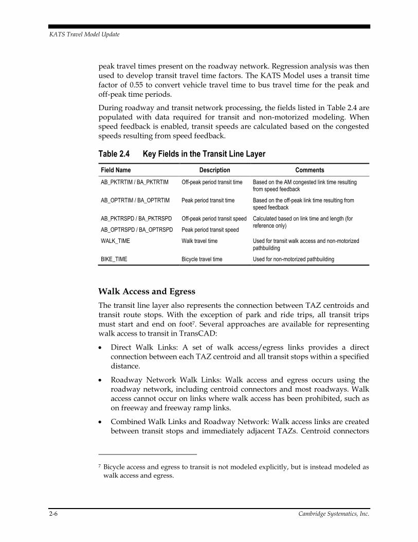
KATS Travel Model Update
2-6 Cambridge Systematics, Inc.
peak travel times present on the roadway network. Regression analysis was then used to develop transit travel time factors. The KATS Model uses a transit time factor of 0.55 to convert vehicle travel time to bus travel time for the peak and off-peak time periods.
During roadway and transit network processing, the fields listed in Table 2.4 are populated with data required for transit and non-motorized modeling. When speed feedback is enabled, transit speeds are calculated based on the congested speeds resulting from speed feedback.
Table 2.4 Key Fields in the Transit Line Layer
Field Name Description Comments
AB_PKTRTIM / BA_PKTRTIM Off-peak period transit time Based on the AM congested link time resulting from speed feedback
AB_OPTRTIM / BA_OPTRTIM Peak period transit time Based on the off-peak link time resulting from speed feedback
AB_PKTRSPD / BA_PKTRSPD Off-peak period transit speed Calculated based on link time and length (for reference only)
AB_OPTRSPD / BA_OPTRSPD Peak period transit speed
WALK_TIME Walk travel time Used for transit walk access and non-motorized pathbuilding
BIKE_TIME Bicycle travel time Used for non-motorized pathbuilding
Walk Access and Egress
The transit line layer also represents the connection between TAZ centroids and transit route stops. With the exception of park and ride trips, all transit trips must start and end on foot7. Several approaches are available for representing walk access to transit in TransCAD:
Direct Walk Links: A set of walk access/egress links provides a direct connection between each TAZ centroid and all transit stops within a specified distance.
Roadway Network Walk Links: Walk access and egress occurs using the roadway network, including centroid connectors and most roadways. Walk access cannot occur on links where walk access has been prohibited, such as on freeway and freeway ramp links.
Combined Walk Links and Roadway Network: Walk access links are created between transit stops and immediately adjacent TAZs. Centroid connectors
7 Bicycle access and egress to transit is not modeled explicitly, but is instead modeled as walk access and egress.

KATS Travel Model Update
Cambridge Systematics, Inc. 2-7
and the roadway layer are used to facilitate walk access and egress for TAZs that are not immediately adjacent to transit stops.
The KATS Model connects TAZs to transit stops using the combined walk access link and roadway network approach. This approach allows direct access to transit stops adjacent to TAZs while representing the increased walk distance to and from zones that are near transit stops but not directly adjacent. An example of transit walk paths from two different zones to a specified transit stop is demonstrated in Figure 2.3.
Figure 2.3 Example Walk Access Paths
The model automatically draws walk links from TAZ centroids to the five closest stops within a 0.5 mile radius. Walk access links are created in the transit line layer and are not present in the roadway line layer. A facility type value of 10 prevents use of walk access links by vehicles. A walk speed of 3 mph is assigned to all links on which walk access is permitted.
Timed Transfers
For transfers at most locations, the transfer wait time is computed as one-half the headway of the route being boarded. However, the bus system is timed to provide quick transfers at the Kalamazoo Transportation Center. The KATS Model applies a lower transfer time at this location using a different transfer time value stored on the network node layer. The node field PULSE will override the default transfer time for all transfers occurring at a node if it contains a positive value. In the calibrated base year model, the PULSE field is populated at the downtown transfer center with a value of 10 minutes, which is 20 minutes faster than the maximum computer generated time of 30 minutes under existing conditions (half the 60 minute maximum bus headway). When testing future
Example Paths:
Green Path: 0.25 miles / 5 minute walk
Purple Path: 1.25 miles / 25 minute walk

KATS Travel Model Update
2-8 Cambridge Systematics, Inc.
scenarios this timed transfer functionality can be applied should other transit centers be considered elsewhere around Kalamazoo.
Drive Access
While the KMetro system does not currently feature any formal park and ride lots, it may be desirable to use the model to evaluate park and ride options in the future. The KATS Model has been set up to accommodate park and ride facilities, but the park and ride mode is inactive in the base year.
If desired, park and ride facilities can be included in the transit networks by identifying specific nodes that are to be designated as park and rides. These park and ride nodes are added to the PNR field on the input network node layer, designated by the number 1. All transit stops placed at a park and ride node allow park and ride or drive access to transit.
Drive access connectivity is only provided in the out bound direction from TAZs to route stops. By following this convention, it is possible to limit drive access to transit to the production (or home) end of each trip. Because transit riders do not typically have access to a vehicle at the attraction (or non-home) end of a trip, transit egress is limited to the walk mode. This is consistent with Mode choice, transit pathbuilding and transit assignment as they are all performed in Production/Attraction format rather than Origin/Destination format.
When activated, drive access to transit is modeled using centroid connectors and roadway links. Zone to park and ride travel times are computed using peak and off-peak travel times from the roadway network.
2.3 TRANSIT PATHBUILDING Transit networks are created in TransCAD for use with the transit path builder (Pathfinder). Pathfinder is a program unique to the TransCAD software and builds best paths using a generalized cost approach. Each component of a transit trip is converted into a common unit, allowing application of different weights to each trip component. Trip components include things like walk access time, wait time, fare, in vehicle travel time, etc. Pathfinder weights have been set for consistency with coefficients in the mode choice model.
Pathfinder evaluates all possible transit paths between each zone pair and identifies the path with the lowest generalized cost. Path components considered by the Pathfinder setup in the KATS Model are listed along with path building weights in Table 2.5.
The travel time and cost variables are converted for inclusion in the generalized cost calculation using a value of time of $11.06. This value of time is based on half the median regional income as reported by the American Community Survey. The median annual household income of $46,000 has been converted to dollars per hour using an assumption of 2,080 work hours in a year. The

KATS Travel Model Update
Cambridge Systematics, Inc. 2-9
Pathfinder weights and the value of time are held constant for all model applications, whether current or future year.
Table 2.5 Transit Path Building Weights
Variable Description Weight
Walk Access Time Time spent walking from the production TAZ centroid to the transit stop (for walk access trips only)
2.5
Drive Access Time Time spent driving from the production TAZ centroid to a park and ride (for drive access trips only)
2.5
Drive Access Cost Auto operating cost associated with drive access (for drive access trips only)
1
Initial Wait Time Time spent waiting for the first bus to arrive, computed as one-half of the route headway.
2.5
In-Vehicle Travel Time Time spent riding or waiting in a transit vehicle 1
Transfer Wait Time Time spent walking between stops for a transfer 2.5
Transfer Walk Time Time spent walking between stops for a transfer 2.5
Transfer Penalty Time Additional transfer penalty (calibration parameter) 1
Egress Walk Time Time spent walking from the transit stop to the attraction TAZ centroid
2.5
Fare Transit fare paid for the trip 1
Note: Travel time variables are converted for consistency with cost variables using a value of time of $11.06, which is 1/2 the regional median income as reported by the American Community Survey.


KATS Travel Model Update
Cambridge Systematics, Inc. 3-1
3.0 Traffic Analysis Zones
Traffic analysis zones (TAZs) are boundaries that contain socioeconomic data used as the foundation for trip-making in the travel model. The TAZ layer is formatted as a polygon layer in TransCAD’s GIS structure. The TAZs are attached to the networks using zone centroids and centroid connectors that allow travelers access to the transportation system by simulating local and neighborhood streets8.
Socioeconomic data are the input activity-based information providing the foundation for trip-making in the travel model. Data includes information about retail, service, medical, and basic employment types and households by income groups and household sizes. Employment data for 2010 are based on data from private employer datasets that were obtained and processed by MDOT, while household data are based on Census 2010 data. Employment data has undergone extensive review by KATS staff based on knowledge of the area. Forecast socioeconomic data was prepared by KATS staff, based on MDOT statewide model forecast data and local knowledge.
3.1 TRAFFIC ANALYSIS ZONE STRUCTURE TAZs are ideally but not always sized and shaped to provide a relatively homogeneous amount and type of activity within each zone. TAZ delineations traditionally follow the natural and manmade boundaries that tend to segregate different land uses. These boundaries include water features, roads, railroads, and other lines that form logical boundaries. Jurisdictional and census boundaries do not always make for good TAZ definitions because they can be arbitrary in relation to the needs of the model, but they are usually desirable for data development and reporting functions.
The definition of TAZs has implications throughout the travel model. For roadway model components, TAZ resolution affects the amount of precision that can be achieved when loading vehicles onto the collector and arterial roadway network. Improved precision can be obtained by increasing detail in the roadway network, TAZ structure, and socioeconomic data. The desire for increased detail must however be balanced with the ability to develop and maintain the data at the increased level of detail.
8 Additional information on TAZ delineation can be found in A recommended Approach to Delineating Traffic Analysis Zones in Florida, prepared in September 2007 for the Florida Department of Transportation Systems Planning Office.

KATS Travel Model Update
3-2 Cambridge Systematics, Inc.
The TAZ layer is a polygon layer that divides the modeling area into TAZs and external stations. While this layer is useful in developing socioeconomic data and as a guide when placing centroids and centroid connectors, it is not used directly by the travel model algorithms. Instead, TAZs are represented by centroids in the roadway network file. The methodology used for placement of centroids is discussed more fully in Chapter 1 of this report, along with the methodology used to assign area type designations to each TAZ.
The TAZ-based data are stored in a separate table rather than directly in the TAZ polygon layer. This allows data from different sources to be modified quickly and efficiently without the need to maintain multiple TAZ layers.
Intermediate and output data at the TAZ level is stored in TransCAD binary table files or matrix files in the output directory for each scenario. Each of these output files can be joined to the TAZ polygon layer or to centroids in the roadway network. TAZ-based intermediate and output data includes terminal times, trip productions and attractions, trip matrices, and skim (shortest path) matrices. TAZ-based output data are discussed in detail in following chapters describing the respective model components.
The TAZ layer has been redefined based on Census 2010 block geography. TAZs were created by merging census blocks into logical groups. Census blocks were split into different TAZs on only rare occasions when census blocks did not serve as logical or reasonable TAZ boundaries. TAZ boundaries were developed through a coordinated review effort involving MDOT, KATS, and the consultant. The TAZ boundaries were reviewed for compatibility with the roadway network, appropriate sizing given the activity density (i.e. compactness versus TAZ size) and land use homogeneity using aerial photography. The resulting TAZ structure is shown in Figure 3.1 and Figure 3.2. TAZ numbers were defined in ranges for various political boundaries as listed in Table 3.1. TAZ numbers are not sequential, allowing for new TAZs to be added in a jurisdiction while maintaining the current numbering scheme.
Table 3.1 TAZ Numbering Ranges
TAZ Number Range Political Boundary
101 - 106 Waverly TWP
201 - 215 Paw Paw TWP
301 - 312 Village of Paw Paw
401 - 408 Almena TWP
501 - 530 Antwerp TWP
601 - 607 Village of Lawton
701 - 711 Alamo TWP
801 - 827 Oshtemo TWP
901 - 923 Texas TWP

KATS Travel Model Update
Cambridge Systematics, Inc. 3-3
TAZ Number Range Political Boundary
1001 - 1008 Prairie Ronde TWP
1101 - 1116 Cooper TWP
1201 - 1224 Kalamazoo (west) TWP
1301 - 1313 Kalamazoo (east) TWP
1401 - 1405 City of Parchment
1501 - 1543 City of Kalamazoo (northwest)
1601 - 1613 City of Kalamazoo (northeast)
1701 - 1794 City of Kalamazoo (south)
1801 - 1855 City of Portage
1901 - 1916 Schoolcraft TWP
2001 - 2005 Village of Schoolcraft
2101 - 2103 Village of Vicksburg (west)
2201 - 2202 Village of Vicksburg (east)
2301 - 2312 Richland TWP
2401 - 2405 Village of Richland
2501 - 2540 Comstock TWP
2601 - 2605 City of Galesburg
2701 - 2710 Pavilion TWP
2801 - 2810 Brady TWP
2901 - 2910 Ross TWP
3001 - 3004 Village of Augusta
3101 - 3101 Fort Custer
3201 - 3214 Charleston TWP
3301 - 3307 Climax TWP
3401 - 3405 Village of Climax
3501 - 3504 Wakeshma TWP
9001 - 9024 External Stations


KATS Travel Model Update
Cambridge Systematics, Inc. 3-5
Figure 3.1 Traffic Analysis Zones

KATS Travel Model Update
3-6 Cambridge Systematics, Inc.
Figure 3.2 Traffic Analysis Zones (urban area detail)
3.2 HOUSEHOLD AND POPULATION DATA Household data is used in the travel model primarily to generate trip productions. As discussed in Chapter 6, trip rates are applied in the model to represent trip-making characteristics that vary by household size, income and number of workers. Generally, trip rates increase as these variables increase.
Household data for 2010 was derived from the 2010 Census data. Because the base year of 2010 coincides with the decennial Census, it was not necessary to

KATS Travel Model Update
Cambridge Systematics, Inc. 3-7
supplement Census data with building permit or other locally maintained data as is done when a model base year does not coincide with a census.
Future year household data was developed by KATS staff, based on local knowledge and MDOT statewide model TAZ forecasts. KATS staff developed separate estimates of population and household growth in each model TAZ.
Figure 3.3 shows the household densities that result from the aggregation of household data into the model’s TAZs for the 2010 base year, with 2045 forecast household density shown in Figure 3.4. Household and population totals for 2010 and 2045 are included in Table 3.2.
Table 3.2 Population and Household Totals
Population Households Average Household
Size
2010 290,251 114,684 2.53
2045 350,186 140,122 2.50
Compound Annual Growth Rate 0.54% 0.54% n/a
Source: Analysis of US Census data, MDOT statewide model forecasts, KATS staff input.


KATS Travel Model Update
Cambridge Systematics, Inc. 3-9
Figure 3.3 Household Density (2010)
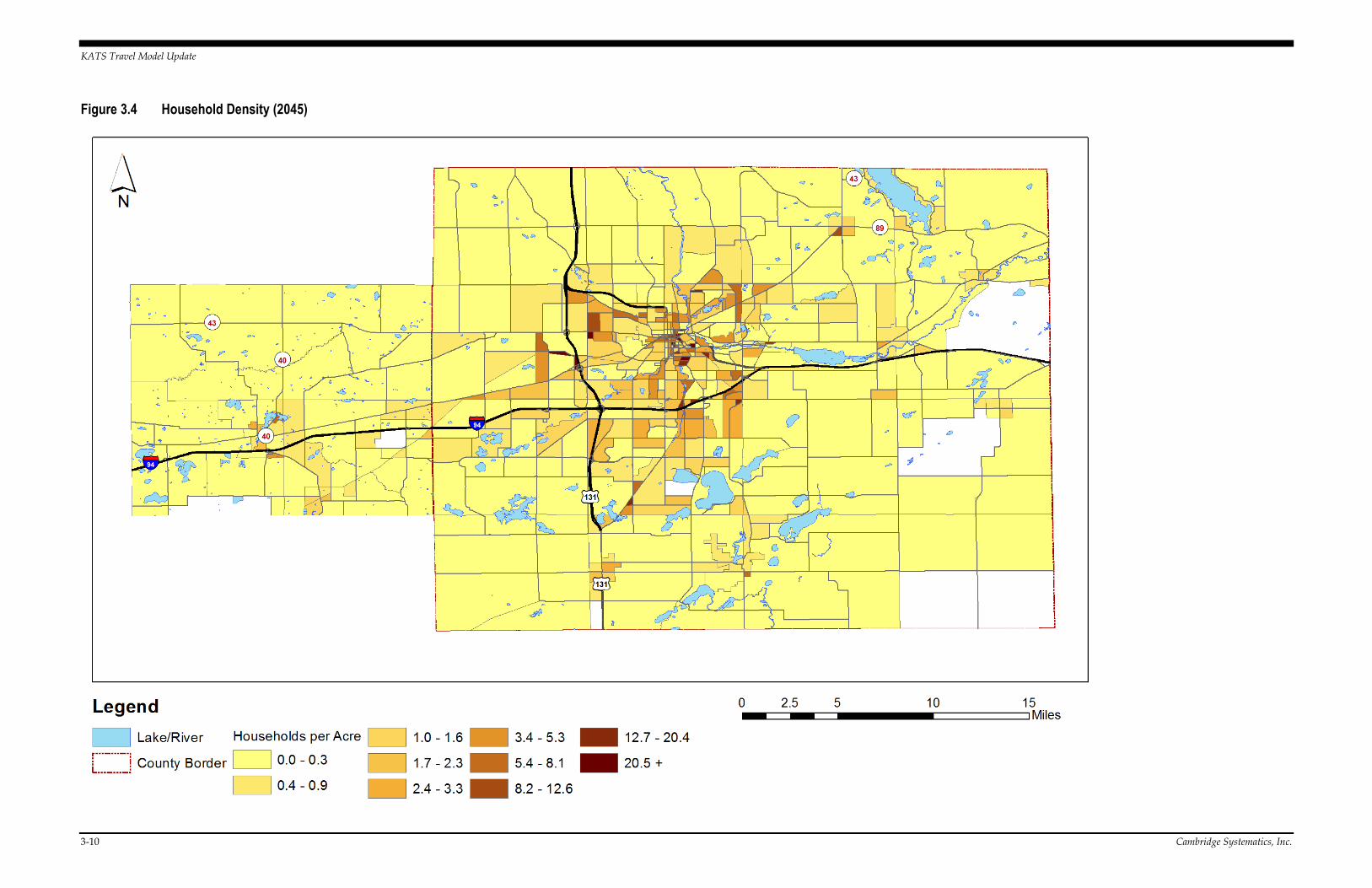
KATS Travel Model Update
3-10 Cambridge Systematics, Inc.
Figure 3.4 Household Density (2045)

KATS Travel Model Update
Cambridge Systematics, Inc. 3-11
3.3 EMPLOYMENT AND ENROLLMENT DATA Employment and enrollment data are used in the travel model primarily as generators of trip attractions. Employment data have been estimated using information from two separate private employer datasets obtained by MDOT, along with school district information and KATS staff review.
A significant amount of manual review and adjustment was necessary to ensure quality. For example, use of multiple source datasets can lead to double-counting of larger employers in the region. KATS staff reviewed records in the employer dataset, eliminating duplicate records and correcting any obvious errors. The resulting employment dataset was then aggregated to the TAZ level.
The school district was not well represented by the private employer datasets. MDOT therefore provided a separate dataset that identified both employment and enrollment at each individual school location in the county. All K-12 school employment was dropped from the private employer datasets and replaced with the more accurate information.
Review of the two major medical centers in Kalamazoo indicated that the private employer datasets did not well represent employment at these locations. Total employment for both Borgess Medical Center and Bronson Methodist Hospital were obtained from American Hospital Association (AHA) reports9. To ensure reasonableness, the AHA reported employment was compared to employment at other hospitals with a similar number of beds. These reports indicated employment totals shown in Table 3.3, which replaced medical employment totals aggregated from the private employer datasets. A small amount of non-medical employees present in the private employee database were retained, as these were assumed to reflect non-hospital activities.
Table 3.3 Hospital Employment Totals
Facility TAZ Medical Employment
Borgess Medical Center 1607 2,206
Bronson Methodist Hospital 1726, 1727 (split evenly)
3,300
Source: AHA Data Viewer reports
Employment data is categorized into retail, service, medical, and basic categories. The traditional non-retail employment category is separated into basic and service categories, with the service category further split into medical and
9 http://www.ahadataviewer.com

KATS Travel Model Update
3-12 Cambridge Systematics, Inc.
general service. This breakdown acknowledges the differences in trip rates for different types of employers. Separation of the basic employment type allows representation of the lower overall trip rates generally observed at basic employment locations, while separation of the medical category allows better representation of trip rates at hospitals and medical campuses.
Basic jobs, also known as production-distribution, are those that are based on outside dollars flowing into the local economy and include industries that manufacture and/or produce goods locally for export outside the region. They include manufacturing, mining, utilities, transportation, warehousing, and others. Retail jobs include retail trade, post offices, and food service. Service jobs include finance, insurance, real estate, and public administration. Medical jobs include hospitals, ambulatory health care services, nursing, and residential care facilities.
The private employment datasets include North American Industrial Classification Standard (NAICS) codes for each employer. Employment type is generally defined by two-digit NAICS codes, but three-digit NAICS codes are used to represent types of employment that need to be treated differently for travel modeling purposes. While post offices are generally defined as basic employment, the model treats these jobs as service employment since they operate a service counter and P.O. boxes as well as mail delivery services. Food service, although often defined as service employment, is categorized as retail in the travel model because the high trip generation associated with restaurants is more characteristic of retail establishments having higher trips per employee than typical service businesses. Finally, while social assistance jobs are generally categorized as medical employment, they are categorized as service employment for purposes of the travel model. The correspondence between NAICS codes and employment types is shown in Table 3.4. Table 3.5 summarizes the 2010 and 2045 employment data for the modeling area.
Employment forecasts were developed using growth assumptions extracted from the statewide model. Statewide model growth assumptions were adjusted and disaggregated by KATS staff. Conversely, school enrollment forecasts were increased uniformly for all schools based on the regional rate of household growth.
Results showing 2010 employment density by TAZ are shown in Figure 3.5 with 2045 employment density by TAZ shown in Figure 3.6.

KATS Travel Model Update
Cambridge Systematics, Inc. 3-13
Table 3.4 NAICS Code to Employment Type Correspondence
NAICS Code Industry Model Category
11 Agriculture, Forestry, Fishing & Hunting Basic
21 Mining, Quarrying, and Oil and Gas Extraction Basic
22 Utilities Basic
23 Construction Basic
31 Manufacturing Basic
32 Manufacturing Basic
33 Manufacturing Basic
42 Wholesale Trade Basic
44 Retail Retail
45 Retail Retail
48 Transportation and Warehousing Basic
49 Transportation and Warehousing Basic (1)
51 Information Service
52 Finance and Insurance Service
53 Real Estate and Rental and Leasing Service
54 Professional, Scientific, and Technical Services Service
55 Management of Companies and Enterprises Service
56 Administrative and Support and Waste Management and Remediation Services
Service
61 Educational Services Service
62 Health Care and Social Assistance Medical (2)
71 Arts, Entertainment, and Recreation Service
72 Accommodation and Food Services Service (3)
81 Other Services (except Public Administration) Service
92 Public Administration Service
Notes: (1) 491, postal service, is classified as service employment. (2) 624, social assistance, is included in service. (3) 722, food service, is included in retail.

KATS Travel Model Update
3-14 Cambridge Systematics, Inc.
Table 3.5 2010 and 2045 Employment Data
Retail
Employment Service
Employment Basic
Employment Medical
Employment Total
Employment
2010 32,393 56,026 41,503 16,928 146,850
2045 35,620 66,987 44,446 22,566 169,619
Compound Annual Growth Rate
0.27% 0.51% 0.20% 0.82% 0.41%
Source: Analysis of private employer datasets, school district employment data, AHA data viewer reports for base year. Analysis of MDOT statewide model forecasts and KATS staff input for 2045.
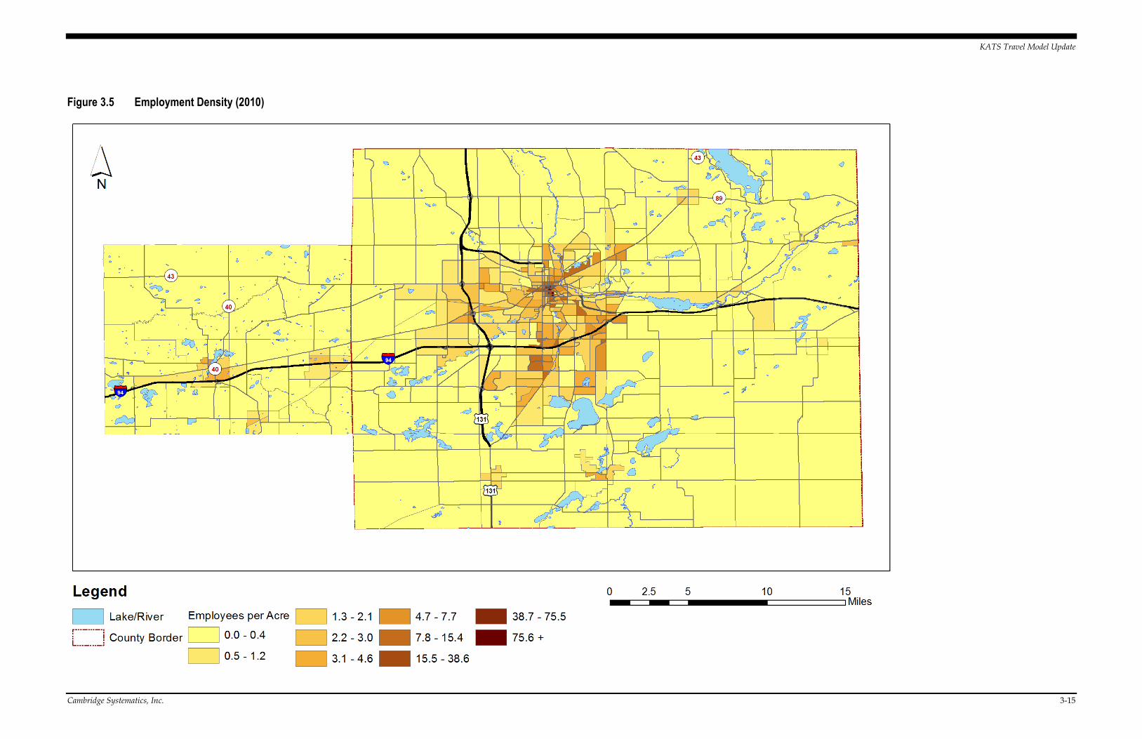
KATS Travel Model Update
Cambridge Systematics, Inc. 3-15
Figure 3.5 Employment Density (2010)
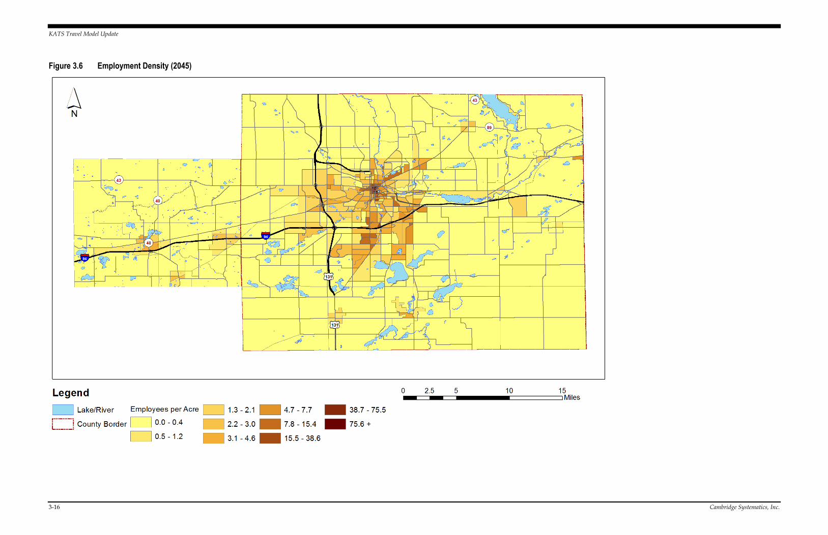
KATS Travel Model Update
3-16 Cambridge Systematics, Inc.
Figure 3.6 Employment Density (2045)

KATS Travel Model Update
Cambridge Systematics, Inc. 4-1
4.0 External Travel
In addition to the internal-internal trips that occur entirely within the modeling area, the model must include external travel from outside of the region. Trips with one end inside the modeling area and the other outside of the area are called internal-external (IE) or external-internal (EI) trips. Through trips, or external-external (EE) trips, are those that pass through the modeling area without stopping or with only short convenience stops. There was no external station survey data available for the KATS study area, so a series of assertions were made to develop the following information.
External travel is modeled explicitly at the 24 external stations where roadways cross the model boundary as shown in Figure 4.1.


KATS Travel Model Update
Cambridge Systematics, Inc. 4-1
Figure 4.1 External Station Locations
KATS Travel Model Update
4-2 Cambridge Systematics, Inc.

KATS Travel Model Update
Cambridge Systematics, Inc. 4-1
4.1 EXTERNAL STATION VOLUMES The first step in estimating external travel for the model is to determine the average weekday traffic at each location in the base year. Traffic counts were collected from MDOT, the KATS traffic count database, and the Van Buren County Road Commission (VBCRC) at each of the external station locations. There were 4 external stations without any available count data. Two locations are classified as collector streets, so a base volume of 500 vehicles per day has been assumed for each of these locations. Two additional external stations with no count data available are classified as minor arterials. At these locations, approximate volumes were obtained from the Michigan Statewide Model.
Once the count data was assembled, it was necessary to determine the share of each total daily traffic count that represented EE trips and the share going to IE/EI trips. Often there are external station surveys conducted where data about origin, destination and trip purpose are assembled. There was no external station survey available for the KATS model area, so the project team reviewed each station along with the Michigan Statewide Model and the corresponding roadway functional class to make an assertion about the share of EE trips. Table 4.1 shows traffic count data along with EE trip shares for each external station.
Table 4.1 External Station Volumes and IE/EE Splits
ID Description Count Source Count Volume % EE
9001 131 N of County Line MDOT 40,667 40%*
9002 12th St N of County Line Asserted 500 0%
9003 Douglas Ave N of County Line KATS 4620 0%
9004 Riverview Dr N of County Line KATS 2,332 0%
9005 M89 N of County Line Statewide Model 5,800 70%*
9006 M43 N of County Line MDOT 14,207 0%
9007 40th N of County Line MDOT 1,890 60%
9008 M89 E of County Line Statewide Model 8,800 50%
9009 M96 E of County Line MDOT 8,370 0%
9010 I94 E of County Line MDOT 51,422 30%
9011 Mercury Drive E of County Line KATS 3,373 0%
9012 W Ave W of County Line KATS 513 0%
9013 24th S of County Line Asserted 500 0%
9014 US131 S of County Line MDOT 29,462 25%
9015 652 S of 72nd VBCRC 501 0%
9016 M40 S of 72nd MDOT 6,790 20%

KATS Travel Model Update
4-2 Cambridge Systematics, Inc.
9017 M51 S of 72nd MDOT 6,201 40%
9018 I94 W of 46th St MDOT 29,294 35%
9019 Red Arrow Highway W of 56th Ave VBCRC 6,175 20%
9020 CR374 W of 46th St VBCRC 1,327 0%
9021 M43 W of 46th St MDOT 6,430 30%
9022 CR665 N of 24th Ave VRCRC 2,532 30%
9023 M40 N of 24th Ave MDOT 7,090 30%
9024 Ravine Rd N of County Line KATS 5,183 0%
Source: Analysis of KATS Travel Model External Station traffic count data and MDOT Statewide Model Data. Statewide model data based on analysis provided by MDOT dated 6/3/2014. * EE shares for stations 9001 and 9005 were increased from initial statewide model values during model validation based on analysis of localized traffic count data.
External-Internal Trips
Once the share of EE trips was determined, the remaining trips from each external station were treated as IE/EI trips. Two possible options for treatment of IE/EI trips were considered for the KATS model.
4. Separate IE/EI Trip Purpose: With this approach, the IE and EI trips are treated as a separate trip purpose, usually with all productions modeled at external stations and attractions modeled at internal zones. With this approach, IE/EI trip attractions must be explicitly generated for internal zones. This simplifies the modeling process, but can result in an unrealistically even distribution of IE/EI trip ends throughout the modeling area.
5. Combined internal and IE/EI Trip Purposes: With this approach, trip ends at external stations are specified by purpose and direction (i.e., production vs. attraction). IE/EI trip totals are then distributed along with internal trips, allowing the density of IE/EI trips to vary by TAZ.
The KATS Model has been implemented using the combined internal and IE/EI approach. To support this method, it was necessary to define trip purpose and direction at each external station. In addition, it was necessary to convert vehicle trips based on count data to person trips for compatibility with the internal trip purposes. The KATS Model trip purposes are Home Based Work (HBW), Home Based Shop (HBS), Home Based Other (HBO), Work Based Other (WBO) and Other Based Other (OBO). The share by trip purpose at external stations was inferred based on the approximate overall shares of trips by purpose from the KATS travel model. Average auto occupancy by trip purpose was calculated based on the drive alone and shared ride assumptions that are further described in Chapter 8 of this report. Resulting shares of IE/EI trips by trip purpose are shown in Table 4.2 along with average auto occupancy values. During model validation, the IE/EI person trip totals were scaled to correct any inconsistencies

KATS Travel Model Update
Cambridge Systematics, Inc. 4-3
between resulting external station model volumes and traffic counts, with the resulting IE/EI and EE and totals shown in Table 4.3.
Table 4.2 External Trip Share and Auto Occupancy by Purpose
HBW HBS HBO WBO OBO
Share of Total 17% 12% 44% 8% 19%
Average Auto Occupancy (persons / vehicle)
1.11 2.54 1.91 1.23 2.20
Source: Approximate share of internal trips by purpose; drive alone and shared ride mode share calibration targets.
Table 4.3 Resulting IE/EI and EE trip totals for 2010 and 2045
ID Description 2010
IE/EI Trips 2010
EE Trips 2045
IE/EI Trips 2045
IE/EI Trips
9001 131 N of County Line 31,920 16,268 39,000 19,878
9002 12th St N of County Line 719 0 879 0
9003 Douglas Ave N of County Line 6,692 0 8,177 0
9004 Riverview Dr N of County Line 3,363 0 4,109 0
9005 M89 N of County Line 2,601 4,060 3,179 4,960
9006 M43 N of County Line 20,531 0 25,085 0
9007 40th N of County Line 1,783 758 2,178 928
9008 M89 E of County Line 6,347 4,402 7,755 5,378
9009 M96 E of County Line 12,363 0 15,106 0
9010 I94 E of County Line 51,534 15,426 62,964 18,850
9011 Mercury Drive E of County Line 4,857 0 5,933 0
9012 W Ave W of County Line 740 0 905 0
9013 24th S of County Line 726 0 888 0
9014 US131 S of County Line 31,611 7,366 38,622 9,002
9015 652 S of 72nd 723 0 883 0
9016 M40 S of 72nd 8,047 1,358 9,831 1,662
9017 M51 S of 72nd 5,351 2,480 6,538 3,028
9018 I94 W of 46th St 19,322 14,648 23,606 17,898
9019 Red Arrow Highway W of 56th Ave 7,118 1,236 8,698 1,508
9020 CR374 W of 46th St 1,914 0 2,340 0
9021 M43 W of 46th St 6,467 1,930 7,902 2,360
9022 CR665 N of 24th Ave 2,552 760 3,118 930
9023 M40 N of 24th Ave 7,130 2,128 8,711 2,602

KATS Travel Model Update
4-4 Cambridge Systematics, Inc.
9024 Ravine Rd N of County Line 7,474 0 9,132 0
Finally, it is important to understand whether a trip has the production end internal to the KATS study area or the attraction end internal to the study area. The relationship of productions to attractions by purpose was asserted from based on assumptions about commute patterns to and from the KATS area. At all locations except two, 80% of home-based trips are assumed to have a production outside of the KATS study area and an attraction inside the KATS study area, with the remaining 20% having the production end inside of the KATS area. For WBO trips, 80% are assumed to have a production in the KATS area, while 50% of OBO trips are assumed to have a production in the KATS area. Two external stations were treated differently as they are on major roadways leading to nearby cities that experience a higher level of interaction with the Kalamazoo area (Grand Rapids and Battle Creek). For these two stations, numbers 9001 and 9010, the production and attraction split was assumed to be 50% for all trip purposes.
External-External Trips
For the external stations identified as having EE trips, a seed matrix of the likelihood for interaction between the four stations was created. This initial relationship was adjusted using an iterative proportional factoring procedure (IPF) so that entering and exiting vehicle totals are consistent with the traffic counts and EE trip shares. The initial seed matrix is shown in Table 4.4, with the resulting vehicle trip matrix for the E-E trips shown in Table 4.5.

KATS Travel Model Update
Cambridge Systematics, Inc. 4-5
Table 4.4 External Trip Seed Matrix
ID 9001 9005 9007 9008 9010 9014 9016 9017 9018 9019 9021 9022 9023
9001 0 0 0 0.5 1 1 0.5 0.5 1 0.5 0.5 0 0
9005 0 0 0 1 0.1 0.1 0 0 0.1 0 0 0 0
9007 0 0 0 1 0.5 0.5 0 0 0.5 0 0 0 0
9008 0.5 1 1 0 0 0.5 0 0 0.5 0 0 0 0
9010 1 0.1 0.5 0 0 1 0.5 0.5 2 0.5 0.5 0.5 0.5
9014 1 0.1 0.5 0.5 1 0 0 0 1 0.5 0.5 0.5 0.5
9016 0.5 0 0 0 0.5 0 0 0 0.5 0.3 0.3 0.3 0.3
9017 0.5 0 0 0 0.5 0 0 0 0.5 0.3 0.3 0.3 0.3
9018 1 0.1 0.5 0.5 2 1 0.5 0.5 0 0 0 0 0.5
9019 0.5 0 0 0 0.5 0.5 0.3 0.3 0 0 0 0 0.3
9021 0.5 0 0 0 0.5 0.5 0.3 0.3 0 0 0 0.3 0.5
9022 0 0 0 0 0.5 0.5 0.3 0.3 0 0 0.3 0 0
9023 0 0 0 0 0.5 0.5 0.3 0.3 0.5 0.3 0.5 0 0
Table 4.5 External Trip Table
ID 9001 9005 9007 9008 9010 9014 9016 9017 9018 9019 9021 9022 9023
9001 0 0 0 462 2,457 1,327 275 502 2,418 285 407 0 0
9005 0 0 0 1,215 323 174 0 0 318 0 0 0 0
9007 0 0 0 130 173 93 0 0 170 0 0 0 0
9008 462 1,215 130 0 0 139 0 0 253 0 0 0 0
9010 2,457 323 173 0 0 738 153 279 2,693 159 226 188 324
9014 1,327 174 93 139 738 0 0 0 727 86 122 101 175
9016 275 0 0 0 153 0 0 0 151 18 25 21 36
9017 502 0 0 0 279 0 0 0 275 32 46 38 66
9018 2,418 318 170 253 2,693 727 151 275 0 0 0 0 319
9019 285 0 0 0 159 86 18 32 0 0 0 0 38
9021 407 0 0 0 226 122 25 46 0 0 0 31 107
9022 0 0 0 0 188 101 21 38 0 0 31 0 0
9023 0 0 0 0 324 175 36 66 319 38 107 0 0

KATS Travel Model Update
4-6 Cambridge Systematics, Inc.
4.2 EXTERNAL STATION FORECASTS Unlike internal travel, the external travel model is not based directly on socioeconomic data inputs. Instead, traffic volumes at external stations are an explicit travel model input. To develop forecast year external station volumes, the IE/EE percentages, trip purpose percentages, and directional percentages are held constant. External station volume totals are then increased at a rate consistent with the assumed population growth. Resulting external trip totals for 2045 are shown in Table 4.3

KATS Travel Model Update
Cambridge Systematics, Inc. 5-7
5.0 Household Survey Processing
In 2004 and 2005, MDOT and its consultants conducted the Michigan Travel Counts (MITC) project, a comprehensive household travel data collection program. This was a household-based travel diary survey that recorded trip-making for approximately 14,000 households statewide, including 291 households within Kalamazoo County and 33 in Van Buren County. This was a 48-hour survey in which trip-making was recorded for each participating household over a 2-day period.
The MITC serves as the foundation for estimation of the trip generation model, development of trip distribution and mode choice calibration targets, and estimation of time of day model parameters in the KATS Model. The survey includes information collected from participating households including demographic information such as household income and size, as well as detailed diaries of all travel conducted by participating household members during the survey period.
Prior to delivery for use in the KATS model update, MDOT processed the household survey dataset and performed significant quality control review of the contents. MDOT also geocoded each location in the survey, producing geographic coordinates for each trip end for all recorded trips. The survey process and results are documented in the document 2004-2005 Comprehensive Household Travel Data Collection Program, MI Travel Counts, Final Report (August 31, 2005).
5.1 SURVEY WEIGHTING AND EXPANSION Prior to using the household travel survey to develop model parameters, it was necessary to compare the demographic and geographic distribution of survey records to the observed distributions obtained from American Community Survey (ACS) data and the Census. Ideally, distributions of surveyed households will match the distributions obtained from ACS and the Census. However, varying response and participation by different groups often lead to differences between surveyed and observed distributions. Such differences, in turn, could impact the calculation of key metrics such as total trips, trips by purpose, trip distribution, time-of-day of travel, and mode splits.
Therefore, it is essential that a set of weighting and expansion factors be created to reconcile survey records with observed distributions. These factors simultaneously weight the survey records so that distributions match observed data, and expand the survey records to represent the total

KATS Travel Model Update
5-8 Cambridge Systematics, Inc.
population of the KATS region. Expansion factors were only developed for households located within the KATS modeling area. Development of these weighting and expansion factors is described below.
Comparison to Observed Distributions
The Census bureau provides household and person tabulations in the ACS data and Census summaries. The 2008 – 2012 5-year dataset and 2010 Census, were used to expand the survey data, since this range is centered around the 2010 base year used in the KATS Model. Because the Census is a full count, the ACS totals were all matched to the Census totals. The ACS was used to obtain distributions that were not included in the available Census summaries.
Distribution of survey records and Census/ACS data were compared for each of the following variables:
Household Income (3 variables, ACS),
Household Size (5 variables, Census),
Number of Workers (4 variables, ACS), and
Number of Vehicles (4 variables, ACS).
Household survey and Census/ACS distributions are shown in Table 5.1 through Table 5.4. Each of these tables also includes the expanded totals. A normalized sampling factor greater than 1 indicates an under-sampled category, while a factor less than 1 indicates an over-sample. As expected, the household survey captured sufficient records in most of the reviewed categories. Two categories (0-vehicle households and 3+ worker households) have relatively small samples, but represent a small portion of the regional population. This suggests that caution should be used when evaluating results for these categories.
Table 5.1 Survey and ACS Comparison: Household Income
Income Group Household Survey
Records Household Survey
Records (%) ACS
Records ACS Records
(%) Normalized
Sampling Factor
Low ($0 - 20k) 55 18% 23,831 22% 1.20
Middle ($20 - 60k) 129 42% 43,781 40% 0.94
High ($60k +) 123 40% 43,148 39% 0.97
Total 307 100% 110,760 100% 1.00
Note: Household records with missing income data are excluded from this table.

KATS Travel Model Update
Cambridge Systematics, Inc. 5-9
Table 5.2 Survey and Census Comparison: Household Size
Household Size Household Survey
Records Household Survey
Records (%) Census Records
Census Records (%)
Normalized Sampling Factor
1 90 28% 31,982 29% 1.04
2 117 36% 38,508 35% 0.96
3 56 17% 16,788 15% 0.88
4 36 11% 13,976 13% 1.14
5+ 25 8% 9,506 9% 1.11
Total 324 100% 110,760 100% 1.00
Table 5.3 Survey and ACS Comparison: Household Vehicles
Number of Autos Household Survey
Records Household Survey
Records (%) ACS
Records ACS Records
(%) Normalized
Sampling Factor
0 20 6% 8,130 7% 1.19
1 109 34% 39,529 36% 1.06
2 134 41% 43,589 39% 0.95
3+ 61 19% 19,511 18% 0.94
Total 324 100% 110,760 100% 1.00
Table 5.4 Survey and ACS Comparison: Household Workers
Number of Workers
Household Survey Records
Household Survey Records (%)
ACS Records
ACS Records (%)
Normalized Sampling Factor
0 81 25% 32,192 29% 1.15
1 132 41% 42,533 38% 0.94
2 95 30% 30,690 28% 0.92
3+ 13 4% 5,345 5% 1.21
Total 321 100% 110,760 100% 1.00
Expansion Factor Development
The variables defined above result in 204 unique combinations of household categories (e.g., 4+ size, 2+ workers, 2 vehicles, and medium income). Sufficient data are not available in the household survey data to produce expansion factors at the individual 204-cell level. Consequently, a raking procedure or iterative proportional fitting (IPF) process was implemented to establish expansion weights in an iterative fashion. Resulting factors produce household totals within 1% of the target ACS values.
The ACS data were used to establish univariate or marginal totals for control variable categories. The household survey data were then tabulated by the control variable categories to provide an initial estimate of the joint distribution. The joint distribution cells were factored to match marginal

KATS Travel Model Update
5-10 Cambridge Systematics, Inc.
totals sequentially for each of the 4 control variables (i.e., income, household size, number of vehicles, and number of workers). Factors were applied iteratively until expanded marginal totals matched the target values developed from ACS data.
Expansion factors were developed so that when applied, the sum of expansion factors for all household records in a category will sum to the number of observed households. These household expansion factors are applicable to every person and trip record for use in survey analysis. Weighted household survey summaries and ACS distributions are shown in Table 5.5 through Table 5.8.
Table 5.5 Expansion Summary: Household Income
Income Group Household Survey
Records Household Survey
Records (%) ACS Records ACS Records (%)
Low ($0 - 20k) 22,236 21% 23,831 22%
Middle ($20 - 60k) 40,925 40% 43,781 40%
High ($60k +) 40,391 39% 43,148 39%
Total 103,552 100% 110,760 100%
Note: Household records with missing income data are excluded from this table.
Table 5.6 Expansion Summary: Household Size
Household Size Household Survey
Records Household Survey
Records (%) Census Records Census Records (%)
1 32,058 29% 31,982 29%
2 38,515 35% 38,508 35%
3 16,759 15% 16,788 15%
4 13,940 13% 13,976 13%
5+ 9,489 9% 9,506 9%
Total 110,760 100% 110,760 100%
Table 5.7 Expansion Summary: Household Vehicles
Number of Autos Household Survey
Records Household Survey
Records (%) ACS Records ACS Records (%)
0 8,162 7% 8,130 7%
1 39,600 36% 39,529 36%
2 43,525 39% 43,589 39%
3+ 19,472 18% 19,511 18%
Total 110,760 100% 110,760 100%

KATS Travel Model Update
Cambridge Systematics, Inc. 5-11
Table 5.8 Expansion Summary: Household Workers
Number of Workers
Household Survey Records
Household Survey Records (%) ACS Records ACS Records (%)
0 32,192 29% 32,192 29%
1 42,533 38% 42,533 38%
2 30,690 28% 30,690 28%
3+ 5,345 5% 5,345 5%
Total 321 100% 110,760 100%
If a single expansion factor was applied to all records, each survey record would reflect approximately 342 households. Weighted expansion factors range from 182.7 to 544.5. These expansion factors are reasonable, with normalized expansion factors ranging from 0.53 to 1.59. Normalized weights close to 1.0 are most common, as demonstrated by the histogram in Figure 5.1.
Figure 5.1 Number of survey records by normalized weight
Use of Additional Records
The MI Travel Counts survey dataset contains 324 household records within the KATS modeling area, for an equivalent of 3,152 un-expanded trip records made by study area households. This information may be sufficient for use in some analysis such as estimation of trip attraction rates, development of trip distribution calibration targets, and creation of drive alone/shared ride mode

KATS Travel Model Update
5-12 Cambridge Systematics, Inc.
choice calibration targets. However, the 324 sampled households do not provide a sufficient sample size for estimation of cross-classified trip production rates.
Production rate cross-classification analysis requires analysis for 67 individual categories (6 trip purposes along with 4, 9, or 15 household types depending on trip purpose). Household samples from outside of the KATS modeling area were added to the dataset for analysis tasks requiring additional data. Discussions with KATS and MDOT staff identified several areas similar in size and character to the Kalamazoo area. Areas included in the borrowed dataset were:
Small Urban Modeled Areas (SUMAs, region code 7);
Transportation Management Areas (TMAs, region code 6); and
Washtenaw County.
These additional records were only used where records within the KATS area were insufficient for analysis. The larger dataset includes 4,336 households. Records from outside of the KATS area were not expanded, so analysis was performed in a manner that allows for use of unexpanded data.
5.2 TRIP PURPOSES After review of survey data, MDOT’s Urban Model Improvement Program (UMIP) documents, and discussion with the project team, the trip purposes listed below were identified for inclusion in the updated KATS Model.
Home-Based Work (HBW): Trips between a traveler’s residence and workplace.
Home-Based Shop (HBS): Shopping trips starting or ending at the traveler’s residence.
Home-Based School (HBSc): Trips made by students between home and a K-12 school.
Home-Based University (HBU): Trips made by university students and visitors between home and a traditional 4-year university.
Home-Based Other (HBO): All remaining trips starting or ending at the traveler’s residence.
Work-Based Other (WBO): Trips starting or ending at the workplace, but with neither end at the traveler’s residence.
Other-Based Other (OBO): Trips that do not start or end at the traveler’s residence or workplace.
A trip purpose was assigned to each of the records present in the household survey dataset. Trip purpose is defined based on the origin and destination

KATS Travel Model Update
Cambridge Systematics, Inc. 5-13
place type as shown in Table 5.9. The resulting numbers of trips by purpose are shown in Table 5.10.
During processing of survey data, each trip was identified as either a production to attraction trip, or an attraction to production trip. For home-based trip purposes, the trip production end was identified as the trip maker’s home. For WBO trips, the trip production end was identified as the trip maker’s workplace or the work-related location if the trip was not made to or from the primary workplace. For OBO trips, the trip production end was identified as the trip origin.
Table 5.9 Trip Purpose Identification
Production Place Type Attraction Place Type Trip Purpose
Home Workplace HBW
Home Shopping HBS
Home School (K-12) HBSc
Home University HBU
Home Other non-home HBO
Workplace Workplace WBO
Workplace Non-home and Non-work WBO
Non-home and Non-work Non-home and Non-work OBO
Notes: Other non-home includes childcare, eat out, personal business, religious/community, social, recreation, accompany another person, and pick-up/drop-off passenger. Trips with an activity of “turn around” are excluded from analysis.
Table 5.10 Number of Trips by Purpose
Trip Purpose
Number of Trips (Study Area)
Percent of Trips (Study Area)
Number of Trips (with borrowed data)
Percent of Trips (with borrowed data)
HBW 424 13% 6,600 17%
HBS 224 7% 3,469 9%
HBSc 227 7% 3,384 9%
HBU 22 1% 245 1%
HBO 848 27% 12,170 31%
WBO 295 9% 3,772 10%
OBO 1,112 35% 9,040 23%
Total 3,152 100% 38,435 100%
Note: Study area values are weighted and expanded. Values with borrowed data are not weighted or expanded.

KATS Travel Model Update
5-14 Cambridge Systematics, Inc.
5.3 TAZ IDENTIFICATION The household travel survey contained latitude and longitude coordinates for each household and for each place visited. In some cases, the geocoding process used to convert address data provided by survey respondents into geographic coordinates either failed, or placed records at a central zip code location. In such cases, survey records that were unsuccessfully geocoded were still used in the analysis, specifically where the geographic location of the record was not required. But the unsuccessfully geocoded records had to be dropped from analysis that required geo-location of trip-ends. All records with valid coordinates were matched to a TAZ for use in the KATS Model analysis.

KATS Travel Model Update
Cambridge Systematics, Inc. 6-1
6.0 Trip Generation
Trip generation is the first phase of the traditional 4-step travel demand modeling process. It identifies the trip ends (productions and attractions) that correspond to the places where activities occur as represented by socioeconomic data (e.g., households, employment). Productions and attractions are estimated for each Traffic Analysis Zone (TAZ) by trip purpose, and then balanced at the regional level so that total productions and attractions are equal. In some cases, production and attraction allocation sub-models are applied to better represent the geographic distribution of trip-ends. The resulting productions and attractions by trip purpose and TAZ are subsequently used by the Trip Distribution model to estimate zone-to-zone travel patterns.
The trip generation model is defined such that trips are produced at home and are generally attracted to other places of activity (employment). The terms “productions” and “attractions” are the fundamental variables for defining the trip ends associated with travel. Productions generally occur at the home end of a trip; and attractions are typically associated with places of employment. Some exceptions are described in the following sections, but this method of defining productions and attractions is generally used for trips internal to the modeling area.
The trip generation model is applied by multiplying socioeconomic data variables (i.e., household and employment totals) by a set of trip rates for each TAZ. The results of this multiplication are the number of trip-ends per zone. University special generator totals are added to the results separately. For most trip purposes, the total number of attractions are factored at the regional level so that the total number of regional attractions is the same as the total number of regional productions. One exception is the HBU trip purpose, for which productions are scaled to match total attractions.
6.1 TRIP PRODUCTIONS Trip production rates represent the number of trips produced by each household in the modeling area. Productions for home-based trip purposes reflect trip-ends that occur at the household. For non home-based trips, trip productions occur at other non-home locations, but are first generated based on household data. This allows the model to reflect non home-based travel as a function of the total number of households in the region.
Income Group Definitions
The household survey asked participants to identify their income in one of 10 ranges. For travel model development, it is necessary to collapse these

KATS Travel Model Update
6-2 Cambridge Systematics, Inc.
categories into a smaller number of groups based on survey availability, trip rate characteristics, and mode share characteristics.
Large increases in trip rates are seen at the $20,000 and $60,000 levels, suggesting that these would be logical income group delimiters. Transit share is highest for households with incomes less than $20,000, with minimal transit use observed for higher income households. After consideration of trip rates and mode shares, low, medium and high income groups were identified as shown below in Table 6.1.
Table 6.1 Trip Rates by Income Range
Income Range Total Trips per
Household HBW Trips per
Household Transit Share
Income Group
Less than $10k 7.44 0.44 9.5% Low
$10k to $20k 5.73 0.53 10.3%
$20k to $30k 9.10 1.24 0%
Medium $30k to $40k 7.20 1.53 0%
$40k to $50k 12.18 1.41 0%
$50k to $60k 11.85 1.33 0%
$60k to $75k 15.75 1.86 0.9%
High $75k to $100k 12.24 2.34 0%
$100k to $125k 13.89 2.39 0%
$125k or more 10.00 1.91 0%
All Income Groups 10.58 1.49 1.2%
Notes: Information is for households within the KATS modeling area. Records with missing or partial income or data are not included in this table. Incomes are in 2005 dollars. Income group definitions using 2012 ACS data are slightly different, as described further in section 7.3.
Cross Classified Production Rates
The KATS Model uses a cross-classified trip production model, which computes trip production rates for each trip purpose based on household attributes. Examples include trip rates that vary by household income group and size, or by household income and number of autos. Based on a review of MDOT’s Urban Model Improvement Program (UMIP) documents, past experience, and discussions with KATS and MDOT staff, the trip rate variables for use in the KATS Model are defined below:
Work Related Trips (HBW and WBO): Household income and number of workers
Other non-university trips (HBS, HBO, and OBO): Household income and size
School (K-12) and university trip productions are discussed separately in the school and university section of this chapter.
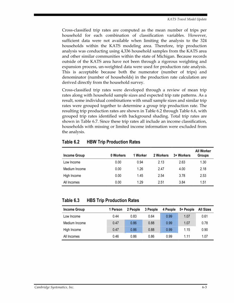
KATS Travel Model Update
Cambridge Systematics, Inc. 6-3
Cross-classified trip rates are computed as the mean number of trips per household for each combination of classification variables. However, sufficient data were not available when limiting the analysis to the 324 households within the KATS modeling area. Therefore, trip production analysis was conducting using 4,336 household samples from the KATS area and other similar communities within the state of Michigan. Because records outside of the KATS area have not been through a rigorous weighting and expansion process, un-weighted data were used for production rate analysis. This is acceptable because both the numerator (number of trips) and denominator (number of households) in the production rate calculation are derived directly from the household survey.
Cross-classified trip rates were developed through a review of mean trip rates along with household sample sizes and expected trip rate patterns. As a result, some individual combinations with small sample sizes and similar trip rates were grouped together to determine a group trip production rate. The resulting trip production rates are shown in Table 6.2 through Table 6.6, with grouped trip rates identified with background shading. Total trip rates are shown in Table 6.7. Since these trip rates all include an income classification, households with missing or limited income information were excluded from the analysis.
Table 6.2 HBW Trip Production Rates
Income Group 0 Workers 1 Worker 2 Workers 3+ Workers All Worker
Groups
Low Income 0.00 0.94 2.13 2.63 1.30
Medium Income 0.00 1.26 2.47 4.00 2.18
High Income 0.00 1.45 2.54 3.78 2.53
All Incomes 0.00 1.29 2.51 3.84 1.51
Table 6.3 HBS Trip Production Rates
Income Group 1 Person 2 People 3 People 4 People 5+ People All Sizes
Low Income 0.44 0.83 0.64 0.99 1.07 0.61
Medium Income 0.47 0.86 0.88 0.99 1.07 0.78
High Income 0.47 0.86 0.88 0.99 1.15 0.90
All Incomes 0.46 0.86 0.86 0.99 1.11 1.07

KATS Travel Model Update
6-4 Cambridge Systematics, Inc.
Table 6.4 HBO Trip Production Rates
Income Group 1 Person 2 People 3 People 4 People 5+ People All Sizes
Low Income 1.19 1.84 3.43 4.05 4.08 1.87
Medium Income 1.28 2.56 3.46 5.06 6.27 2.95
High Income 1.28 2.56 3.46 5.29 7.15 3.80
All Incomes 1.25 2.50 3.46 5.14 6.64 4.16
Table 6.5 WBO Trip Production Rates
Income Group 0 Workers 1 Worker 2 Workers 3+ Workers All Worker
Groups
Low Income 0.00 0.59 0.61 1.00 0.61
Medium Income 0.00 0.82 1.35 1.60 1.11
High Income 0.00 0.84 1.88 2.39 1.77
All Incomes 0.00 0.80 1.70 2.13 0.95
Table 6.6 OBO Trip Production Rates
Income Group 1 Person 2 People 3 People 4 People 5+ People All Sizes
Low Income 0.76 1.46 2.13 2.86 3.92 1.33
Medium Income 0.85 1.91 2.61 3.54 5.11 2.18
High Income 0.85 1.91 2.61 4.06 5.51 2.87
All Incomes 0.82 1.87 2.56 3.81 5.25 3.09
Table 6.7 Trip Production Rate Summary
Income Group HBW HBS HBO WBO OBO Home-Based
Total Total
Low Income 1.30 0.61 1.87 0.61 1.33 3.78 5.71
Medium Income 2.18 0.78 2.95 1.11 2.18 5.92 9.20
High Income 2.53 0.90 3.80 1.77 2.87 7.22 11.86
All Incomes 1.51 1.07 4.16 0.95 3.09 6.74 10.77

KATS Travel Model Update
Cambridge Systematics, Inc. 6-5
6.2 TRIP ATTRACTIONS Attraction rates define the ends of trips that occur at locations other than the trip-maker’s home. For home-based trips, the attraction end of a trip occurs at a non-residential location, or occasionally at another person’s home. For WBO trips, trip productions occur at the trip maker’s workplace and the trip attraction occurs at the non-work end of the trip. For OBO trips, the trip production and attraction are synonymous with trip origin and destination. For non-home-based trip purposes, allocation models and special procedures are used to properly locate the production and attraction end of each trip.
Attraction Variables
Trip attractions are computed based on employment by type, along with total households. Household variables such as income, size, and number of workers are not considered in the trip attraction models because only a small portion of trip attractions occur at households. TAZ household totals were obtained from the US Census, with employment data obtained from Claritas and Hoovers. Employment data were categorized into four employment types using the correspondence shown in Table 6.8.

KATS Travel Model Update
6-6 Cambridge Systematics, Inc.
Table 6.8 NAICS Code to Employment Type Correspondence
Two-Digit NAICS Code Industry Description
Model Employment
Type
11 Agriculture, Forestry, Fishing & Hunting Basic
21 Mining, Quarrying, and Oil and Gas Extraction Basic
22 Utilities Basic
23 Construction Basic
31 Manufacturing Basic
32 Manufacturing Basic
33 Manufacturing Basic
42 Wholesale Trade Basic
44 Retail Retail
45 Retail Retail
48 Transportation and Warehousing Basic
49 Transportation and Warehousing Basic (1)
51 Information Service
52 Finance and Insurance Service
53 Real Estate and Rental and Leasing Service
54 Professional, Scientific, and Technical Services Service
55 Management of Companies and Enterprises Service
56 Administrative and Support and Waste Management and Remediation Services
Service
61 Educational Services Service
62 Health Care and Social Assistance Medical (2)
71 Arts, Entertainment, and Recreation Service
72 Accommodation and Food Services Service (3)
81 Other Services (except Public Administration) Service
92 Public Administration Service
Notes: (1) NAICS code 491 – Postal Service is included in service instead of basic. (2) NAICS code 624 – Social Assistance is included in service instead of medical. (3) NAICS code 722 – Food Service is included in retail instead of service.
Classified Attraction Rates
Trip attraction rates were developed using a classification model, which divides the total number of expanded and weighted tip attractions from the household survey by an attraction variable. This approach requires identification of a land use variable (i.e., either employment type or household) for each trip attraction in the household survey. While an initial
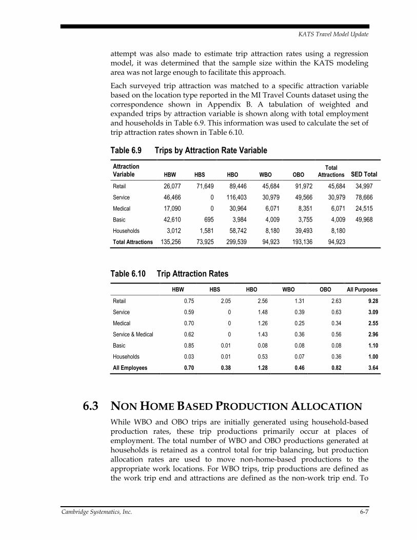
KATS Travel Model Update
Cambridge Systematics, Inc. 6-7
attempt was also made to estimate trip attraction rates using a regression model, it was determined that the sample size within the KATS modeling area was not large enough to facilitate this approach.
Each surveyed trip attraction was matched to a specific attraction variable based on the location type reported in the MI Travel Counts dataset using the correspondence shown in Appendix B. A tabulation of weighted and expanded trips by attraction variable is shown along with total employment and households in Table 6.9. This information was used to calculate the set of trip attraction rates shown in Table 6.10.
Table 6.9 Trips by Attraction Rate Variable
Attraction Variable HBW HBS HBO WBO OBO
Total Attractions SED Total
Retail 26,077 71,649 89,446 45,684 91,972 45,684 34,997
Service 46,466 0 116,403 30,979 49,566 30,979 78,666
Medical 17,090 0 30,964 6,071 8,351 6,071 24,515
Basic 42,610 695 3,984 4,009 3,755 4,009 49,968
Households 3,012 1,581 58,742 8,180 39,493 8,180
Total Attractions 135,256 73,925 299,539 94,923 193,136 94,923
Table 6.10 Trip Attraction Rates
HBW HBS HBO WBO OBO All Purposes
Retail 0.75 2.05 2.56 1.31 2.63 9.28
Service 0.59 0 1.48 0.39 0.63 3.09
Medical 0.70 0 1.26 0.25 0.34 2.55
Service & Medical 0.62 0 1.43 0.36 0.56 2.96
Basic 0.85 0.01 0.08 0.08 0.08 1.10
Households 0.03 0.01 0.53 0.07 0.36 1.00
All Employees 0.70 0.38 1.28 0.46 0.82 3.64
6.3 NON HOME BASED PRODUCTION ALLOCATION While WBO and OBO trips are initially generated using household-based production rates, these trip productions primarily occur at places of employment. The total number of WBO and OBO productions generated at households is retained as a control total for trip balancing, but production allocation rates are used to move non-home-based productions to the appropriate work locations. For WBO trips, trip productions are defined as the work trip end and attractions are defined as the non-work trip end. To

KATS Travel Model Update
6-8 Cambridge Systematics, Inc.
accommodate this, a set of WBO production allocation rates were developed using the classification analysis described above. Resulting WBO production allocation rates are shown in Table 6.11.
A simpler approach was taken for OBO trips. OBO production allocation rates are identical to OBO attraction rates. This approach is possible because there is no distinct difference between OBO productions and attractions. OBO productions and attractions all occur at non-home, non-work locations.
Table 6.11 WBO Production Allocation Rates
Employment WBO Production Allocation Rate
Retail 1.31
Service 0.39
Medical 0.12
Basic 0.16
All Employees 1.98
6.4 SCHOOL AND UNIVERSITY TRIPS The cross classified trip rates described above account for most travel, but do not include K-12 school trips or trips to traditional 4-year universities. Trips to community colleges and vocational schools are included in the HBO trip purpose. Separate models were developed for the K-12 and university trip purposes.
K-12 School Trips
Home Based School (HBSc) trips are defined as trips by students between home and a school at which the student is enrolled. HBSc trips do not include trips by parents, guardians, or others traveling from home to a school; such trips are included in the HBO trip purpose. Trips between school and a non-home location are included in the WBO or OBO trip purposes, even for school students.
HBSc Production Rates
HBSc trip productions were analyzed in a manner similar to other home-based trip production rates, but were considered using a classification based on the number of children ages 5 through 17 in a household. The number of children per household is a variable present in the household survey data, and is also available at the block level from the Census. Trip production rates by number of children per household are shown in Table 6.12.
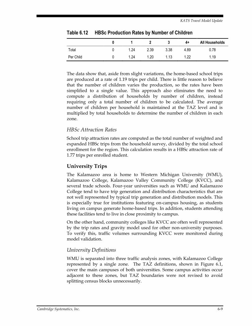
KATS Travel Model Update
Cambridge Systematics, Inc. 6-9
Table 6.12 HBSc Production Rates by Number of Children
0 1 2 3 4+ All Households
Total 0 1.24 2.39 3.38 4.89 0.78
Per Child 0 1.24 1.20 1.13 1.22 1.19
The data show that, aside from slight variations, the home-based school trips are produced at a rate of 1.19 trips per child. There is little reason to believe that the number of children varies the production, so the rates have been simplified to a single value. This approach also eliminates the need to compute a distribution of households by number of children, instead requiring only a total number of children to be calculated. The average number of children per household is maintained at the TAZ level and is multiplied by total households to determine the number of children in each zone.
HBSc Attraction Rates
School trip attraction rates are computed as the total number of weighted and expanded HBSc trips from the household survey, divided by the total school enrollment for the region. This calculation results in a HBSc attraction rate of 1.77 trips per enrolled student.
University Trips
The Kalamazoo area is home to Western Michigan University (WMU), Kalamazoo College, Kalamazoo Valley Community College (KVCC), and several trade schools. Four-year universities such as WMU and Kalamazoo College tend to have trip generation and distribution characteristics that are not well represented by typical trip generation and distribution models. This is especially true for institutions featuring on-campus housing, as students living on campus generate home-based trips. In addition, students attending these facilities tend to live in close proximity to campus.
On the other hand, community colleges like KVCC are often well represented by the trip rates and gravity model used for other non-university purposes. To verify this, traffic volumes surrounding KVCC were monitored during model validation.
University Definitions
WMU is separated into three traffic analysis zones, with Kalamazoo College represented by a single zone. The TAZ definitions, shown in Figure 6.1, cover the main campuses of both universities. Some campus activities occur adjacent to these zones, but TAZ boundaries were not revised to avoid splitting census blocks unnecessarily.

KATS Travel Model Update
6-10 Cambridge Systematics, Inc.
WMU also includes a separate Parkview Campus and a separate Aviation Campus. The Aviation Campus is located outside of the KATS modeling area and the Parkview Campus is located within the KATS modeling area, southwest of the main campus. Because these campuses reflect only a small portion of the overall activity at WMU, they have not been included as separate special generators. However, traffic counts surrounding the Parkview Campus were monitored during model validation to confirm this assumption.
Figure 6.1 WMU and Kalamazoo College Traffic Analysis Zones
Trip Types at Universities
Because universities do no fall into the normal trip patterns used by the model in the remainder of the region, some special considerations are given to trip types at universities. In particular, the Home-Based University (HBU) trip purpose is defined as a trip by a university student or visitor between an off-campus home and any location on the university campus. Trip ends at the university are associated with university faculty and staff, students living on campus, and students and visitors living off campus. Descriptions of how the trip purposes are addressed as university special generators are presented below.

KATS Travel Model Update
Cambridge Systematics, Inc. 6-11
HBW, HBS, and HBO Productions: These production trip ends can occur only for students living on campus.
HBSc Productions and Attractions: These trip ends do not occur at universities.
HBW Attractions and WBO Productions: These trip ends can occur only for University faculty and staff.
WBO Attractions and all OBO Trips: These trip ends can only occur for students and visitors living off campus.
HBS and HBO Attractions: These trip ends cannot occur at the university. All home-based trips to the university by students and visitors are considered HBU trips and all home-based trips to the university by faculty and staff are considered HBW trips.
HBU Productions: Trips within the university campuses are not modeled, so HBU productions cannot occur on campus.
HBU Attractions: HBU attractions can occur only for students and visitors living off campus.
Employment and Enrollment Data
University trip generation is based on 2010 faculty and enrollment totals obtained from each university, along with employment data provided by MDOT. Employment data is summarized Table 6.13 in units of full time equivalent (FTE) employees and does not include third-party vendors or contractors. Enrollment data for each university is summarized in Table 6.14.
Table 6.13 University Employment
WMU Kalamazoo College
Faculty 1,300 103
Staff 1,910 241
Total Employment 3,210 344
Table 6.14 University Enrollment
WMU Kalamazoo College
On-Campus 21,036 852
Off-Campus 5,140 551
Total Enrollment 21,036 1,403
Note: On-campus enrollment is based on on-campus housing capacity at each university.

KATS Travel Model Update
6-12 Cambridge Systematics, Inc.
Special Generator Values
Trips for the university special generators are based on special generator studies conducted for two universities in Northern Colorado in 1999 and 200410. Trip rates developed based on these surveys have been successfully applied in a number of regions. Results from recent studies have been observed to reasonably model activities at other four-year universities when applied based on university specific enrollment and employment data. In the KATS application, traffic count data around the universities was monitored during validation to ensure the special generator values reflect the actual WMU and Kalamazoo College activity. These special generator values replace results that would otherwise be generated by the socio-economic data and trip rates via the traditional trip generation process. They were adjusted up or down based on whether the traffic volumes generated by the KATS model were higher or lower than the observed traffic counts.
Trip rates based on the surveys are defined in units of trips per on-campus student, trips per off-campus student, or trips per employee. Trip rates and resulting special generator values are shown in Table 6.15.
Table 6.15 University Special Generator Values
Trip Purpose
Production / Attraction
Trip Rate Unit
WMU Trip Ends
Kalamazoo College Trip Ends
HBW Productions 0.28 On Campus Students 1,439 852
Attractions 1.47 Total Employment 4,719 344
HBS Productions 0.5 On Campus Students 2,570 852
Attractions 0 n/a 0 0
HBU Productions 0 n/a 0 0
Attractions 3.5 Off Campus Students 55,636 551
HBO Productions 0.9 On Campus Students 4,626 852
Attractions 0 n/a 0 0
WBO Productions 0.37 Total Employment 1,188 344
Attractions 0.19 Off Campus Students 3,020 551
OBO Productions 0.25 Off Campus Students 3,974 551
Attractions 0.25 Off Campus Students 3,974 551
10 Colorado State University Special Generator Study conducted in 1999 and University of Northern Colorado Special Generator Study conducted in 2004.

KATS Travel Model Update
Cambridge Systematics, Inc. 6-13
For WMU, it was necessary to distribute special generator values among the three zones that make up the university. Trips are distributed based on a review of activities occurring in each zone, as shown in Table 6.16.
Table 6.16 Allocation of Special Generators to WMU Zones
TAZ Share of
Productions Share of
Attractions
1506 75% 75%
1704 25% 20%
1705 0% 5%
University Production Allocation
Off-campus HBU productions are modeled at households, and tend to occur near the universities. WMU provided anonymous student address data to assist in development of a HBU production allocation model. These addresses were geocoded and aggregated to the model TAZs using a simple area-based overlay. The calibration parameters in Equation (1) were adjusted iteratively until the resulting production allocation model matched the allocation of geocoded student address data. The resulting calibration parameters were then applied to Kalamazoo College trips as well. The geocoded HBU productions allocated to TAZs are shown in Figure 6.2 as a dot density map.
[𝐴𝑙𝑙𝑜𝑐𝑎𝑡𝑖𝑜𝑛 𝐹𝑎𝑐𝑡𝑜𝑟] = 𝐻𝐻 ∙ 𝛼𝐷𝛽 ∙ 𝑒𝐷𝛾 (1)
Where:
𝐻𝐻 = Number of households in a zone
𝐷 = Distance between the zone and the nearest university zone
𝛼, 𝛽, 𝛾 = Calibration parameters (𝛼 = 35; 𝛽 = −1.05; 𝛾 = −0.006)

KATS Travel Model Update
6-14 Cambridge Systematics, Inc.
Figure 6.2 Home Base University Production Allocation

KATS Travel Model Update
Cambridge Systematics, Inc. 6-15
6.5 TRIP RATE FACTORS Underrepresentation of trip making is common in travel surveys due to under-reporting by survey participants. Experience with household travel surveys conducted in other areas that provided a subset of participants with GPS responders has shown that the commute trips tend to be most accurately reported, while other trips are more likely to be omitted. During model validation, trip rate factors were developed based on a review of modeled volumes as compared traffic count data. The resulting trip rate factors are shown in Table 6.17.
Table 6.17 Trip Rate Factors
Table Column HeadL CBD Urban Suburban Rural
HBW 1.3 1.2 1.5 1.1
HBS 1.5 1.3 1.7 1.1
HBU 1.3 1.2 1.5 1.1
HBSc 1.5 1.3 1.7 1.1
HBO 1.5 1.3 1.7 1.1
WBO Productions 1 1 1.25 1.5
WBO Attractions (1) 1.5 1.3 1.7 1.1
OBO Productions 1 1 1.25 1.5
OBO Attractions 1.5 1.3 1.7 1.1
Note: (1) WBO attraction rate factors are applied to both WBO attraction rates and to WBO production allocation rates.
6.6 TRIP BALANCING Trip productions and attractions were estimated separately by purpose using the trip rates and allocation models previously described. Because the production and attraction models are developed independently, the total number of productions and attractions may not always be identical. The trip balancing process reconciles any differences in production and attraction totals, ensuring conservation of trips in the model.
Balancing depends on the level of confidence associated with the initial estimate of productions and attractions. Since household survey data was used to estimate trip production rates, and US Census based household data is considered more reliable than the employment data, totals for most trip purposes are balanced to productions. HBU trips are balanced to attractions, since university enrollment data is the best available predictor of the number of HBU trips.

KATS Travel Model Update
6-16 Cambridge Systematics, Inc.
6.7 DISAGGREGATION MODELS The model input data includes information about the number of households in each TAZ, along with average household size, average number of workers, median income, and average number of children per household for each TAZ as obtained from US Census and ACS data. The model uses household disaggregation models to estimate the univariate distribution of households by size, number of workers, and by income group for each TAZ. Once these distributions have been estimated, the model uses an iterative proportional factoring process to develop bivariate distributions of households by income and size and by income and number of workers for each TAZ.
Household disaggregation models use known variables to establish a distribution of households by classification. For example, a zone with an average household size of 1 person would be comprised entirely of 1-person households. Conversely, a zone with an average household size of 4 people would be modeled as a combination of 1, 2, 3, 4, and 5+ person households. Distributions are represented by hand-fitted curves based on US Census and ACS data.
The distribution curves must always sum to 100%. For the household size and worker models, the results must be consistent with the input value when averaged. Hand-fitted curves have been adjusted to fit the observed data points, sum to 100%, and produce the appropriate averages.
The household income model is expressed as a percentage of regional income rather than an income value in dollars to allow median income data to be expressed in any unit, so long as the units are consistent for all zones. Data may be input in 2010 dollars, or in some other unit if desired. The KATS Model has been implemented using 2010 dollars.
Household Size Disaggregation Model
The KATS Model trip rates are classified into five household size groups. The portion of households in each group can be approximated for any given TAZ based on the average household size. Disaggregation curves are shown along with Census data in Figure 6.3.

KATS Travel Model Update
Cambridge Systematics, Inc. 6-17
Figure 6.3: Household Size Disaggregation Model
Household Worker Disaggregation Model
The household number of workers model was developed in a manner similar to the household size disaggregation model. Worker information was obtained from the ACS dataset rather than the US Census, and is available at the block group level rather than the block level. Distributions were applied to TAZs based on the household total from the Census block level along with worker data from the block group layer. Disaggregation curves are shown along with ACS data in Figure 6.4.
0%
10%
20%
30%
40%
50%
60%
70%
80%
90%
100%
1
1.2
1.4
1.6
1.8 2
2.2
2.4
2.6
2.8 3
3.2
3.4
3.6
3.8 4
4.2
4.4
4.6
4.8 5
Perc
ent
of
Hosuehold
s
Average Household Size
1 Person Model 2 Person Model 3 Person Model 4 Person Model 5+ Person Model
1 Person HH 2 Person HH 3 Person HH 4 Person HH 5+ Person HH

KATS Travel Model Update
6-18 Cambridge Systematics, Inc.
Figure 6.4 Household Worker Disaggregation Model
Household Income Disaggregation Model
The household income group model was developed in a manner similar to the size and worker disaggregation models, but is based on each TAZ’s median income as a share of the regional median. Income data was obtained from the ACS at the track level. Disaggregation curves for low, medium and high income levels are shown along with Census data in Figure 6.5.
For the 2010 base year model, ACS income groups are specified in 2012 dollars, while household survey data and the resulting trip rates are specified in 2005 dollars. To account for this discrepancy, different income group definitions were used for survey analysis and for model application using ACS-based income data. Table 6.18 shows the 2005 income ranges alongside 2012 CPI adjusted income ranges. For the low income group, the inflation adjusted value is identical to the 2005 value when rounded to the closest available income group cutoff point. The cutoff point between the medium and high income is rounded up to $75,000 dollars when applying the model using 2012 dollars.
0%
10%
20%
30%
40%
50%
60%
70%
80%
90%
100%
0
0.1
0.2
0.3
0.4
0.5
0.6
0.7
0.8
0.9 1
1.1
1.2
1.3
1.4
1.5
1.6
1.7
1.8
1.9 2
2.1
Perc
ent
of H
osuehold
s
Average Numbers of Workers per Household
No Worker 1 Worker 2 Workers 3+ Workers
0 Worker HH 1 Worker HH 3 Worker HH 4+ Worker HH
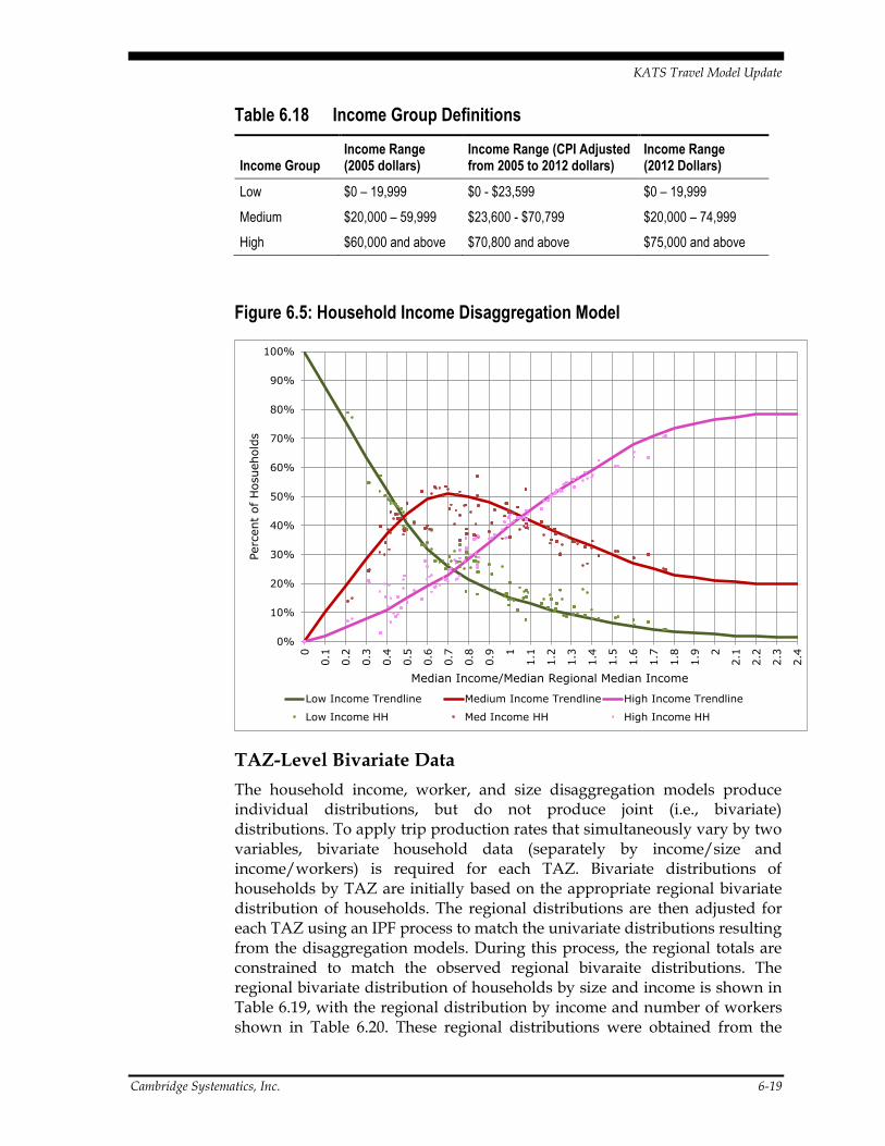
KATS Travel Model Update
Cambridge Systematics, Inc. 6-19
Table 6.18 Income Group Definitions
Income Group Income Range (2005 dollars)
Income Range (CPI Adjusted from 2005 to 2012 dollars)
Income Range (2012 Dollars)
Low $0 – 19,999 $0 - $23,599 $0 – 19,999
Medium $20,000 – 59,999 $23,600 - $70,799 $20,000 – 74,999
High $60,000 and above $70,800 and above $75,000 and above
Figure 6.5: Household Income Disaggregation Model
TAZ-Level Bivariate Data
The household income, worker, and size disaggregation models produce individual distributions, but do not produce joint (i.e., bivariate) distributions. To apply trip production rates that simultaneously vary by two variables, bivariate household data (separately by income/size and income/workers) is required for each TAZ. Bivariate distributions of households by TAZ are initially based on the appropriate regional bivariate distribution of households. The regional distributions are then adjusted for each TAZ using an IPF process to match the univariate distributions resulting from the disaggregation models. During this process, the regional totals are constrained to match the observed regional bivaraite distributions. The regional bivariate distribution of households by size and income is shown in Table 6.19, with the regional distribution by income and number of workers shown in Table 6.20. These regional distributions were obtained from the
0%
10%
20%
30%
40%
50%
60%
70%
80%
90%
100%
0
0.1
0.2
0.3
0.4
0.5
0.6
0.7
0.8
0.9 1
1.1
1.2
1.3
1.4
1.5
1.6
1.7
1.8
1.9 2
2.1
2.2
2.3
2.4
Perc
ent
of H
osuehold
s
Median Income/Median Regional Median Income
Low Income Trendline Medium Income Trendline High Income Trendline
Low Income HH Med Income HH High Income HH

KATS Travel Model Update
6-20 Cambridge Systematics, Inc.
2008-2012 Public Use Micro Sample (PUMS) dataset, which contains data from ACS. Because the PUMS data is only available for large geographic areas called Public Use Micro-data Areas (PUMAs), the bivariate distributions are shown for the entirety of both Kalamazoo and Van Buren Counties combined.
Table 6.19 Bivariate Household Distribution, Household Size
HH Size Low Income
($0 - 20k) Middle Income
($20 - 60k) High Income
($60k +) All Incomes
1-Person 12% 13% 4% 29%
2-Person 5% 16% 14% 35%
3-Person 2% 5% 7% 14%
4-Person 1% 5% 7% 13%
5-Person + 1% 3% 4% 8%
All Sizes 22% 43% 36% 100%
Source: 2008-2012 PUMS Data for PUMAs 02601 and 02602.
Table 6.20 Bivariate Household Distribution, Household Workers
HH Workers Low Income
($0 - 20k) Middle Income
($20 - 60k) High Income
($60k +) All Incomes
0-Worker 7% 7% 1% 16%
1-Workers 11% 18% 8% 37%
2-Workers 3% 14% 21% 37%
3-Workers + 1% 3% 6% 10%
All Worker Categories 22% 43% 36% 100%
Source: 2008-2012 PUMS Data for PUMAs 02601 and 02602.

KATS Travel Model Update
Cambridge Systematics, Inc. 7-1
7.0 Trip Distribution
Trip distribution is the second phase of the traditional 4-step demand model. Trip distribution is the process through which balanced person trip productions and attractions from the trip generation model are apportioned among all zone pairs in the modeling domain. The resulting trip table matrix contains both intrazonal trips (e.g., trips that don’t leave the zone) on the diagonal and interzonal trips in all other zone interchange cells for each trip purpose.
The KATS Model uses a gravity model equation and applies friction factors to represent the effects of impedance between zones. As the impedance (i.e., travel time) between a pair of zones increases, the number of trips between the zone pair decreases as represented by a decreasing friction factor. This is similar to the standard gravity model which assumes that the gravitational attraction between two bodies is directly proportional to their masses. The trip distribution model makes a similar assumption in that the number of trips between two zones is directly proportional to the number of productions and attractions contained in those zones. The gravity model used by trip distribution to estimate the number of trips between each zone pair is defined in the equation below.
n
j
ijijj
ijijj
iij
KFA
KFAPT
1
Where:
Tij = trips from zone i to zone j
Pi = productions in zone i
Ai = attractions in zone j
Kij = K-factor adjustment from i to zone j
i = production zone
j = attraction zone
n = total number of zones
Fij = friction factor (a function of impedance between zones i and j)
K-factors are often used in travel demand models to account for nuances in travel behavior and the transportation system that cannot be accurately modeled with simplified aggregate modeling techniques. They are often applied at the district or jurisdictional level to adjust regional distribution

KATS Travel Model Update
7-2 Cambridge Systematics, Inc.
patterns. They may be applied by trip purpose or for all trips. K-factors are not used in the KATS model.
Friction factors represent the impedance to travel between each zone pair. Friction factors have been calibrated for each trip purpose based on a trip length frequency distribution (TLFD) generated from household survey data and roadway network shortest path matrices.
7.1 PEAK AND OFF-PEAK PERIOD DEFINITIONS Trips occurring during the AM and PM peak hours are distributed based on peak congested speeds and trips occurring during off-peak times are distributed based on off-peak congested speeds. Trip distribution is performed in Production-Attraction (PA) format rather than Origin-Destination (OD) format. This is because the majority of trips in the AM peak hour travel from production to attractions (e.g., to work) and the majority of trips in the PM peak hour travel from attraction to productions (e.g., from work).
To implement trip distribution by time of day, factors representing the portion of trips occurring in the peak (combined AM and PM peak hours) and off-peak (all other times) are necessary. Peak hour trips are further separated in the time of day step prior to traffic assignment using the time of day factors shown in Table 7.1. These time of day factors are based on the mid-point of each trip in the household survey database. They were generated based on data from households in the KATS modeling area supplemented with household survey records from other small and medium sized communities in Michigan.
Table 7.1 Peak and Off-Peak Trip Percentages by Purpose
Time Period HBW HBS HBU HBSc HBO WBO OBO
Peak 7:00 – 8:00 AM and 5:00 – 6:00 PM
29.9% 9.1% 13.1% 35.6% 15.6% 15.0% 7.8%
Off-Peak All other times
70.1% 90.9% 86.9% 64.4% 84.4% 85.0% 92.2%
7.2 ROADWAY NETWORK SHORTEST PATH The impedance portion of the gravity model equation is based on shortest paths between each zone pair. Each shortest path is determined through a process called pathbuilding, which identifies the shortest route between each zone pair. Shortest paths minimize a given variable such as travel time, and cannot pass through other centroid connectors. Various data, such as path distance, can be skimmed along the shortest impedance route. The set of all zone to zone shortest paths is called a shortest path matrix and is sometimes
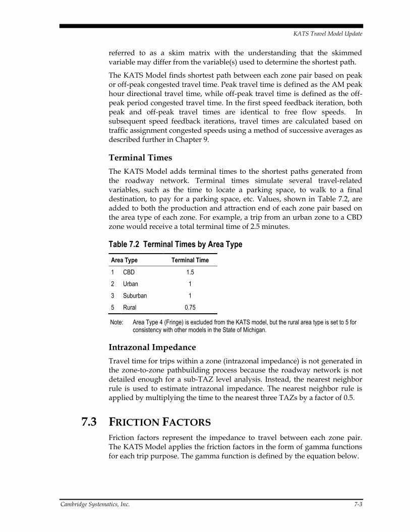
KATS Travel Model Update
Cambridge Systematics, Inc. 7-3
referred to as a skim matrix with the understanding that the skimmed variable may differ from the variable(s) used to determine the shortest path.
The KATS Model finds shortest path between each zone pair based on peak or off-peak congested travel time. Peak travel time is defined as the AM peak hour directional travel time, while off-peak travel time is defined as the off-peak period congested travel time. In the first speed feedback iteration, both peak and off-peak travel times are identical to free flow speeds. In subsequent speed feedback iterations, travel times are calculated based on traffic assignment congested speeds using a method of successive averages as described further in Chapter 9.
Terminal Times
The KATS Model adds terminal times to the shortest paths generated from the roadway network. Terminal times simulate several travel-related variables, such as the time to locate a parking space, to walk to a final destination, to pay for a parking space, etc. Values, shown in Table 7.2, are added to both the production and attraction end of each zone pair based on the area type of each zone. For example, a trip from an urban zone to a CBD zone would receive a total terminal time of 2.5 minutes.
Table 7.2 Terminal Times by Area Type
Area Type Terminal Time
1 CBD 1.5
2 Urban 1
3 Suburban 1
5 Rural 0.75
Note: Area Type 4 (Fringe) is excluded from the KATS model, but the rural area type is set to 5 for consistency with other models in the State of Michigan.
Intrazonal Impedance
Travel time for trips within a zone (intrazonal impedance) is not generated in the zone-to-zone pathbuilding process because the roadway network is not detailed enough for a sub-TAZ level analysis. Instead, the nearest neighbor rule is used to estimate intrazonal impedance. The nearest neighbor rule is applied by multiplying the time to the nearest three TAZs by a factor of 0.5.
7.3 FRICTION FACTORS Friction factors represent the impedance to travel between each zone pair. The KATS Model applies the friction factors in the form of gamma functions for each trip purpose. The gamma function is defined by the equation below.

KATS Travel Model Update
7-4 Cambridge Systematics, Inc.
𝐹𝑖𝑗 = 𝛼𝑡−𝛽𝑒−𝛾𝑡
Where:
𝐹𝑖𝑗 = Friction factor between zones 𝑖 and 𝑗
𝑡 = travel time
𝛼, 𝛽, 𝛾 = calibration parameters
Friction factors for each trip purpose were calibrated by comparing a Trip Length Frequency Distribution (TLFD) generated by the travel model to a TLFD generated from a combination of observed trip OD pairs and the travel model shortest path matrix. Observed OD pairs available for use in trip distribution calibration were limited to trips made by surveyed households located within the KATS modeling area.
The travel model was run iteratively with minor adjustments to calibration parameters alpha, beta, and gamma until the modeled and observed average trip lengths became similar and TLFDs converged to a similar shape. The similarity of the observed and modeled TLFD curves can be quantified by the coincidence ratio, which is defined as the ratio of area under both curves to the area under either curve. The resulting coincidence ratios and average trip lengths are shown in Table 7.3. Observed and calibrated TLFD plots are shown in Figure 7.1 through Figure 7.6. The resulting friction factors are plotted in Figure 7.7, with calibrated gamma function parameters shown in Table 7.4.
A comparison of observed TLFDs for peak and off peak periods shows minimal differences between time periods for all trip purposes. Therefore, separate calibration exercises were not performed for the peak and off-peak time periods. In the KATS model, friction factors for HBW trips were not calibrated separately by income group. There were not sufficient records in the household survey to develop separate TLFDs by income group. Although HBW friction factors do not vary by income group, trip distribution is performed separately for HBW trips made by low, medium, and high income households. This allows income information from the trip generation model to be utilized by the mode choice model.
Table 7.3 Coincidence Ratios and Average Trip Lengths
Trip Purpose Coincidence Ratio Observed Average Trip
Length (minutes) Modeled Average Trip
Length (minutes)
HBW 91.5% 14.3 14.3
HBS 90.2% 9.9 9.9
HBSC 85.7% 8.8 8.7
HBO 86.1% 11.2 11.2
WBO 93.7% 11.3 11.3

KATS Travel Model Update
Cambridge Systematics, Inc. 7-5
Trip Purpose Coincidence Ratio Observed Average Trip
Length (minutes) Modeled Average Trip
Length (minutes)
OBO 89.0% 9.8 9.8
Figure 7.1 HBW Trip Length Frequency Distribution
0
2
4
6
8
10
12
0 10 20 30 40
Perc
en
t o
f Tr
ips
Travel Time (min)
Observed
Model

KATS Travel Model Update
7-6 Cambridge Systematics, Inc.
Figure 7.2 HBS Trip Length Frequency Distribution
Figure 7.3 HBSc Trip Length Frequency Distribution
0
2
4
6
8
10
12
14
16
18
20
0 10 20 30
Perc
en
t o
f Tr
ips
Travel Time (min)
Observed
Model
0
5
10
15
20
25
30
0 10 20 30
Perc
en
t o
f Tr
ips
Travel Time (min)
Observed
Model
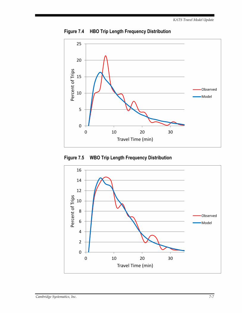
KATS Travel Model Update
Cambridge Systematics, Inc. 7-7
Figure 7.4 HBO Trip Length Frequency Distribution
Figure 7.5 WBO Trip Length Frequency Distribution
0
5
10
15
20
25
0 10 20 30
Perc
en
t o
f Tr
ips
Travel Time (min)
Observed
Model
0
2
4
6
8
10
12
14
16
0 10 20 30
Perc
en
t o
f Tr
ips
Travel Time (min)
Observed
Model

KATS Travel Model Update
7-8 Cambridge Systematics, Inc.
Figure 7.6 OBO Trip Length Frequency Distribution
Figure 7.7 Calibrated Friction Factors
0
5
10
15
20
25
0 10 20 30
Perc
en
t o
f Tr
ips
Travel Time
Observed
Model
0
0.5
1
1.5
2
2.5
3
3.5
4
4.5
5
1 6 11 16 21 26 31 36 41
Fric
tio
n F
acto
r V
alu
e
Travel Time (min)
HBW HBS HBSc HBO WBO OBO
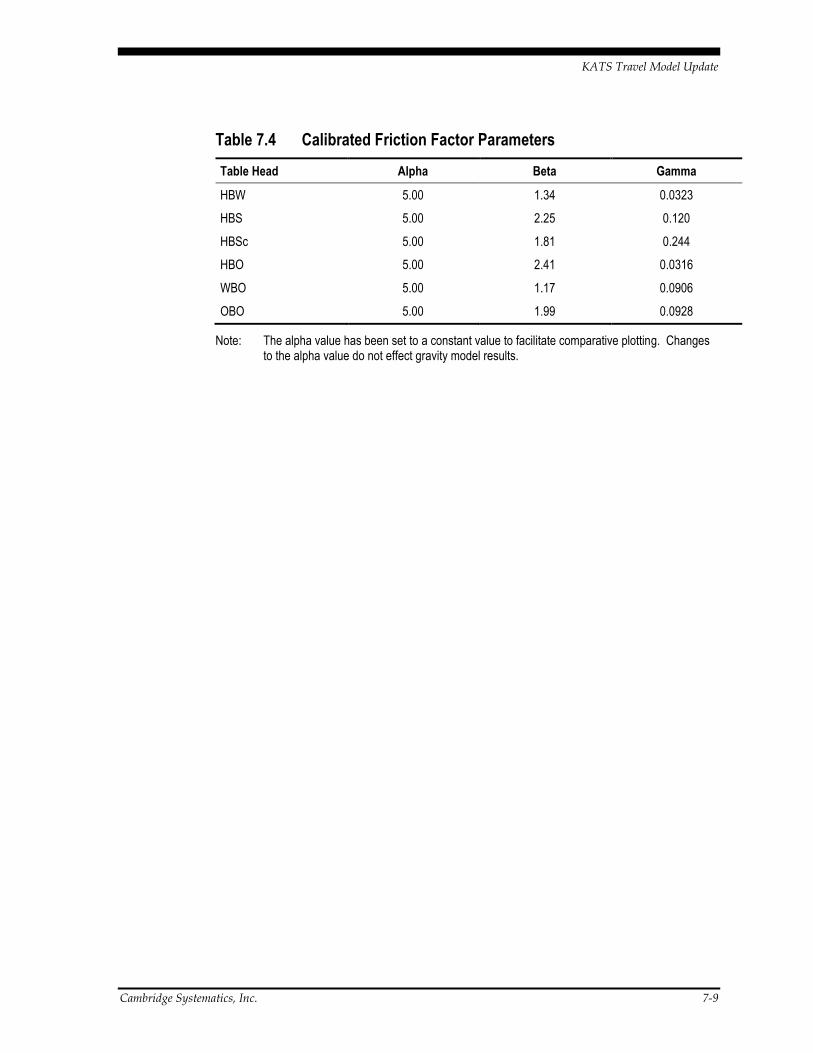
KATS Travel Model Update
Cambridge Systematics, Inc. 7-9
Table 7.4 Calibrated Friction Factor Parameters
Table Head Alpha Beta Gamma
HBW 5.00 1.34 0.0323
HBS 5.00 2.25 0.120
HBSc 5.00 1.81 0.244
HBO 5.00 2.41 0.0316
WBO 5.00 1.17 0.0906
OBO 5.00 1.99 0.0928
Note: The alpha value has been set to a constant value to facilitate comparative plotting. Changes to the alpha value do not effect gravity model results.


KATS Travel Model Update
Cambridge Systematics, Inc. 8-1
8.0 Mode Choice
The KATS Model generates and distributes all person trips including non-motorized, carpool, and transit trips. The mode choice model separates the resulting person trip tables into the drive alone, shared ride (i.e., carpool), transit (walk access and drive access), and non-motorized (bicycle and walk) modes. Information about transit routes provides important input to the mode choice model. The mode choice model also considers trip lengths produced by the gravity model, resulting in sensitivity to higher density and mixed use areas. Such areas will produce shorter trips which are more likely to be made using non-motorized modes. This results in higher non-motorized mode shares in dense mixed use areas and lower non-motorized shares in low density areas with homogenous land use (e.g., urban mixed use areas vs. low and medium density residential neighborhoods). However, the model does not take non-motorized facilities such as sidewalks and bike paths into account for assignment purposes.
The KATS mode choice model uses a nested logit formulation that takes transit service characteristics into account when predicting mode share. The resulting model is not limited to providing a representation of existing conditions, but instead can predict changes in transit ridership resulting from changes to transit service, demographics, and land use patterns.
8.1 OBSERVED MODE SHARES The mode choice model has been calibrated to reproduce observed mode shares. Observed mode share values for auto trips and non-motorized trips are based on data from the 2004/2005 MI Travel Counts household travel survey. Because the 324 households sampled within the KATS modeling area were insufficient to develop reliable estimates of mode share, records from other communities similar in size and character to the Kalamazoo area were included in the analysis11. Total transit trips were obtained from Kalamazoo Transit, with information such as trip purpose and household income based on an on-board rider survey conducted in 201212. The resulting mode share targets are shown in Table 8.1.
Transit trip targets are shown as a total number of trips rather than a percent share of all trips. This allows direct use of transit boarding data. Kalamazoo
11 See Technical Memorandum 5: Household Survey Processing for details about use of additional records.
12 2012 Socio-Economic Survey Report Kalamazoo Metro Transit Line Haul System. Kalamazoo Area Transportation Study. October 2012.

KATS Travel Model Update
8-2 Cambridge Systematics, Inc.
Transit reported an average of 10,113 daily boardings on weekdays in March, April, September, and October of 2010. However, boarding data did not include values for several routes that primarily serve WMU. Boarding estimates for these routes were developed based on results from a preliminary transit assignment. This increases the estimate to 10,644 average daily boardings. Transfer data provided by Kalamazoo Transit indicates an average of 1.45 boardings per trip, resulting in a total of 7,341 daily linked transit trips.
Table 8.1 Mode Share Targets
Trip Purpose Transit Drive Alone Shared Ride Bike Walk
HBW (Low Income) 1,615 70.5% 25.6% 0.1% 3.8%
HBW (Med Income) 220 87.1% 10.3% 1.1% 1.5%
HBW (Hhigh Income) 147 91.8% 6.1% 0.8% 1.3%
HBS 367 61.5% 35.2% 0.4% 2.9%
HBU 2,129 81.1% 10.0% 2.9% 6.0%
HBSc 367 13.5% 72.8% 1.5% 12.2%
HBO 1,468 41.7% 53.2% 0.7% 4.4%
WBO 294 80.4% 15.7% 0.3% 3.7%
OBO 734 31.1% 66.1% 0.2% 2.6%
Total 7,341 n/a n/a n/a n/a
Source: Analysis of MI Travel Counts household survey data
Note: Transit trip targets are shown as total transit trips and non-transit targets are shown as the share of non-transit trips.
8.2 MODE CHOICE MODEL STRUCTURE The KATS mode choice model has been asserted based on guidance from the Federal Transit Administration (FTA) and experience with mode choice modeling in other regions. The asserted approach eliminates the need for extensive data collection and estimation efforts. While model estimation is often useful in large metropolitan areas with extensive transit service, the asserted approach is considered more appropriate for an area with moderate transit service such as the Kalamazoo area.
Logit Model Background
The KATS Model includes a nested logit mode choice model that addresses both motorized and non-motorized modes. Nested logit models represent the current best practice for mode choice modeling. A nested logit model is effectively a series of multinomial logit models applied sequentially from top to bottom. The generalized formulation to compute probability in a multinomial logit model is shown in the equation below. The subsequent

KATS Travel Model Update
Cambridge Systematics, Inc. 8-3
formula shows the probability of selecting mode 1 in the example multinomial logit model in Figure 8.1.
𝑃𝑖 =𝑒𝑢𝑖
∑ 𝑒𝑢𝑚𝑛𝑚=1
Where: 𝑃𝑖 = The probability of using mode 𝑖 𝑢𝑖 = The utility of mode 𝑖 𝑢𝑚 = The utility of mode 𝑚 𝑛 = The number of available modes
𝑃1 =𝑒𝑢1
𝑒𝑢1 + 𝑒𝑢2 + 𝑒𝑢3
Where: 𝑃1 = The probability of using mode 1 𝑢1 = The utility of mode 1 𝑢2 = The utility of mode 2 𝑢3 = The utility of mode 3
Figure 8.1 Example Multinomial Logit Structure
The logit model is based on the concept of utilities (or disutilities) that describe the characteristics of travel by each mode. The utility function can be made up of impedance variables such as travel time, wait time, and cost as well as locational and socioeconomic variables. Each variable is multiplied by a coefficient that describes the relative weight (positive or negative) of each variable. Utility values can also include a mode constant that captures mode preferences that are not measured by the other utility variables. Due to the relative nature of the mode constants, the mode constant for one mode must be set to zero. The standard utility equation is shown below
𝑢𝑖 = 𝑐1 ∙ 𝑥1𝑖 + 𝑐2 ∙ 𝑥2𝑖 + 𝑐3 ∙ 𝑥3𝑖 + ⋯ + 𝑐𝑛 ∙ 𝑥𝑛𝑖 + 𝐾𝑖
Where: 𝑢𝑖 = The utility for mode 𝑖 𝑐1, 𝑐2, 𝑐3, … , 𝑐𝑛 = Mode coefficients for variables 1, 2, 3, … , 𝑛 𝑥1𝑖, 𝑥2𝑖, 𝑥3𝑖, … , 𝑥𝑛𝑖 = Values for variables 1, 2, 3, … , 𝑛 for mode 𝑖
𝐾𝑖 = The mode constant for mode 𝑖
Choice
Mode 1 Mode 2 Mode 3

KATS Travel Model Update
8-4 Cambridge Systematics, Inc.
An example equation for the utility of mode 1 is shown in the equation below. In this simplified example, the utility variables include terminal time, drive time, and auto operating costs.
𝑢1 = 𝑐𝑡𝑒𝑟𝑚𝑖𝑛𝑎𝑙 ∙ 𝑡𝑡𝑒𝑟𝑚𝑖𝑛𝑎𝑙 + 𝑐𝑑𝑟𝑖𝑣𝑒 ∙ 𝑡𝑑𝑟𝑖𝑣𝑒 + 𝑐𝑐𝑜𝑠𝑡 ∙ 𝐶𝑜𝑝𝑒𝑟𝑎𝑡𝑖𝑛𝑔 + 𝐾1
Where: 𝑢1 = The utility for mode 1 𝑐𝑡𝑒𝑟𝑚𝑖𝑛𝑎𝑙 = Mode coefficient for terminal time 𝑐𝑑𝑟𝑖𝑣𝑒 = Mode coefficient for drive time 𝑐𝑐𝑜𝑠𝑡 = Mode coefficient for travel cost 𝑡𝑡𝑒𝑟𝑚𝑖𝑛𝑎𝑙 = Trip terminal time 𝑡𝑑𝑟𝑖𝑣𝑒 = Trip drive time 𝐶𝑜𝑝𝑒𝑟𝑎𝑡𝑖𝑛𝑔 = Auto operating cost
𝐾1 = The mode constant for mode 1
The KATS model uses a mode choice structure that nests multiple multinomial choices. At the bottom level of the nested logit structure, utility values are computed using the method described for multinomial application. Utilities for Intermediate modes are computed as a combination of the utilities for the nested modes (i.e., modes below the intermediate mode). Utilities for intermediate modes are based on the natural log of the sum of exponentiated sub-mode utilities. This term, referred to as the “logsum” variable, is computed as shown.
𝐿𝑆𝑖 = ln (∑ 𝑒𝑢𝑗
𝑛
𝑗=1
)
Where: 𝐿𝑆𝑖 = The logsum of intermediate mode 𝑖 𝑢𝑗 = Utility terms for nested mode j
𝑛 = The number of sub-modes under mode 𝑖
Once the logsum variables have been computed for all intermediate modes, mode probabilities are calculated in a manner similar to that described for multinomial logit models. However, for nested modes, utilities are replaced by the product of the logsum and a nesting coefficient as shown in the equation below. The nesting coefficient has a value between 0 and 1, where a nesting value of 0 indicates that sub-modes are identical and do not need to be included as separate modes and a nesting value of 1 indicates that sub-modes are distinctly different and could be represented as separate non-nested modes.
𝑃𝑖 =𝑒𝜃𝑖∙𝐿𝑆𝑖
∑ 𝑒𝜃𝑚∙𝐿𝑆𝑚𝑛
𝑚=1
Where: 𝑃𝑖 = The probability of selecting intermediate mode 𝑖 𝜃𝑖 = The nesting coefficient for intermediate mode 𝑖

KATS Travel Model Update
Cambridge Systematics, Inc. 8-5
𝜃𝑚 = The nesting coefficient for mode m
𝑛 = The number of modes at the same level as mode 𝑖
As an example, the probability of selecting the motorized mode in the example nested model in Figure 8.2 can be expressed as follows.
𝑃𝑚𝑜𝑡𝑜𝑟 =𝑒𝜃𝑡∙𝐿𝑆𝑚𝑜𝑡𝑜𝑟𝑖𝑧𝑒𝑑
𝑒𝜃𝑡∙𝐿𝑆𝑚𝑜𝑡𝑜𝑟 + 𝑒𝜃𝑡∙𝐿𝑆𝑤𝑎𝑙𝑘 + 𝑒𝜃𝑡∙𝐿𝑆𝑏𝑖𝑘𝑒
Where: 𝑃𝑚𝑜𝑡𝑜𝑟 = The probability of selecting the motorized mode 𝜃𝑡 = The top level nesting coefficient 𝐿𝑆𝑚𝑜𝑡𝑜𝑟𝑖𝑧𝑒𝑑 = The logsum for the motorized mode 𝐿𝑆𝑤𝑎𝑙𝑘 = The logsum for the motorized mode
𝐿𝑆𝑏𝑖𝑘𝑒 = The logsum for the bicycle mode
In this example, the logsum variable for both non-motorized modes is very simple to calculate, as the non-motorized modes do not include any additional nests. For example, the logsum for the walk mode can be computed as shown below. This computation is further simplified by the fact that ln(𝑒𝑥) = 𝑥.
𝐿𝑆𝑤𝑎𝑙𝑘 = ln(𝑒𝑢𝑤𝑎𝑙𝑘) = 𝑢𝑤𝑎𝑙𝑘
Figure 8.2 Example Nested Logit Model
KATS Mode Choice Model Definition
The KATS Model uses the nested logit model structure shown in Figure 8.3. This structure first separates trips into auto, transit, and non motorized modes. Transit trips are further separated into walk and drive access, while auto trips are further separated into drive alone and shared ride modes. Non motorized trips are separated into walk and bike modes.
The drive access mode included in the KATS mode choice model is included to allow for future model expandability, as Kalamazoo transit does not currently feature any formal park and ride lots. As presently implemented,
Choice
Motorized
Drive Alone
Shared Ride
Transit
Bicycle
Bicycle
Walk
Walk

KATS Travel Model Update
8-6 Cambridge Systematics, Inc.
the model does not generate drive access trips using designated park and ride lots.
Figure 8.3 KATS Model Choice Model Structure
Utility Functions
Utility functions for each mode shown in the bottom row of the nested logit structure are described in Table 8.2, with associated coefficients shown in Table 8.3. Coefficients asserted for use in the KATS mode choice model are based on the FTA guidance shown in Table 8.4. These tables fully define the utility equations used in the KATS model. For example, the utility equation for the low income shared ride mode can be read from the table and written as shown in the equation below.
𝑼𝑺𝑹,𝑳𝒐𝒘𝑰𝒏𝒄 = −𝟎. 𝟔𝟐𝟒 ∙ 𝑶𝒑𝑪𝒐𝒔𝒕 + −𝟎. 𝟎𝟔𝟓 ∙ 𝑻𝒆𝒓𝒎 + −𝟎. 𝟎𝟐𝟓 ∙ 𝐼𝑉𝑇𝑇 + 𝑲𝑺𝑹
Where:
𝑈𝑠𝑟,𝐿𝑜𝑤𝐼𝑛𝑐 = Utility for shared ride in the low income market segment 𝑂𝑝𝐶𝑜𝑠𝑡 = Total operating cost 𝑇𝑒𝑟𝑚 = Total terminal time 𝐼𝑉𝑇𝑇 = Total in-vehicle travel time 𝐾𝑆𝑅 = Alternative specific constant for shared ride
Auto modes generally include a terminal time, drive time, and auto operating cost. Transit modes include time spent traveling to and from transit stops, time waiting for a bus, time spent in the transit vehicle, and transit fare. Non-motorized modes include travel time and a term measuring density of the TAZ where the trip occurs. All modes also include an alternative specific constant, with the constant value for the drive alone mode set to zero.
Cost coefficients vary by income group. For the low, medium, and medium high income groups, value of time is set to one half of the hourly rate associated with the midpoint of the income range. For non-work trips, the value of time is based on one half the hourly wage associated with the regional median household income. The non-work value of time is consistent
Choice
Auto
Drive Alone
Shared Ride
Transit
Walk Access
Drive Access
Non-Motorized
Walk Bike

KATS Travel Model Update
Cambridge Systematics, Inc. 8-7
with the value of time utilized in the transit pathfinder algorithm and in the traffic assignment step.
All constants and coefficients are applied at the auto/transit level in the nested logit mode choice structure. In model application, coefficients are multiplied by the nesting coefficients of 0.70 to determine values used in utility calculation for individual nodes. Coefficients are specified at the auto/transit level to facilitate comparison to other mode choice models specified at this level.
Alternative specific constants have been calibrated to observed trip values discussed previously. The resulting constants are shown in Table 8.5. Because the Kalamazoo area does not currently feature any formal park and rides, the drive access constants have been asserted as -2 for all purposes. Drive access constants are added to the transit constant in model application.
Table 8.2 Utility Specifications
Mode Drive Alone
Shared Ride
Walk to Transit
Drive to Transit
Walk Bike
Non-Motorized Time
Operating Cost
Terminal Time
In-Vehicle Time
Drive Access Time
Walk Access/Egress Time
Short initial wait (1)
Long initial wait (1)
Transfer wait
Transfer penalty time (2)
Transit Fare
Destination CBD (3) (3) (3) (3)
Attraction Density (3) (3) (3)
Notes: (1) Short initial wait time includes the first 7.5 minutes, while long initial wait time includes any initial wait over 7.5 minutes. (2) Transfer penalty is set to zero in the calibrated model. (3) These terms are included in the model setup, but are currently set to zero.
Table 8.3 Utility Variable Coefficients
Variable Coefficient Value
Non-motorized Time OVTT -0.065
Operating Cost, Cost Segment Coefficient Value of time ($/hr)

KATS Travel Model Update
8-8 Cambridge Systematics, Inc.
Transit Fare Low Income -0.624 $2.40
Med Income -0.156 $9.62
High Income -0.069 $21.63
Non-Work -0.136 $11.06
Terminal Time OVTT -0.065
In-Vehicle Time IVTT -0.025
Walk Access/Egress Time
OVTT -0.065
Short Initial Wait OVTT -0.065
Long Initial Wait IVTT -0.025
Transfer Wait XWAIT -0.050
Transfer Penalty IVTT -0.025
Attraction CBD CBD_Dummy 0 (included for possible future use)
Attraction Density Density Walk: 0.01
All other modes: 0 (included for possible future use)
Note: Coefficients are specified at the auto/transit nest and are scaled by the product of nesting coefficients for application at the bottom level of the mode choice tree.
Table 8.4 FTA Mode Choice Model Coefficient Guidelines
Variable Minimum Coefficient Value Maximum Coefficient Value
In-vehicle travel time -0.03 -0.02
Initial wait time -0.09 -0.04
Second wait time -0.09 -0.04
Walk time -0.09 -0.04
Source: PowerPoint presentation by FTA at TRB 83rd Annual Meeting, Session 501, January 13, 2004.
Table 8.5 Alternative Specific Constants
Trip Purpose Drive Alone Shared Ride Transit Walk Bike
HBW (Low Income) 0 -1.26 0.78 -2.52 -0.45
HBW (Med Income) 0 -1.53 -3.42 -2.52 -0.45
HBW (Hhigh Income) 0 -1.85 -3.63 -2.52 -0.45
HBS 0 -0.39 -3.13 -2.18 -1.70
HBU 0 -1.36 -0.79 -0.43 2.00
HBSc 0 1.18 -0.69 0.30 0.65
HBO 0 0.17 -2.64 -1.36 -0.78
WBO 0 -1.14 -3.57 -2.04 -2.09
OBO 0 0.53 -2.74 -1.83 -1.99

KATS Travel Model Update
Cambridge Systematics, Inc. 8-9
Notes: Walk and bike constants have been calibrated across all income groups due to a low number of samples in individual income categories.
8.3 AUTO OCCUPANCY The mode choice model separates vehicle trips into drive alone and shared ride. For drive alone, auto occupancy is explicitly defined as 1 occupant. For the shared ride mode, average vehicle occupancy is expected to be higher than 2 and has been computed based on household travel survey data. Auto occupancy for trips in shared ride vehicles are listed in Table 8.6, with overall average auto occupancy shown for reference. The average auto occupancy values for shared ride trips are used to convert person trips by travel model into vehicle trips for assignment to the roadway network.
Table 8.6 Average Auto Occupancy by Trip Purpose
Trip Purpose All Vehicles Shared Ride
HBW 1.11 2.22
HBS 1.53 2.46
HBU 1.13 2.22
HBSc 2.54 2.82
HBO 1.91 2.62
WBO 1.23 2.42
OBO 2.20 2.77
Total 1.76 2.66
Source: Analysis of MI Travel Counts household survey data

KATS Travel Model Update
9-10 Cambridge Systematics, Inc.
9.0 Time of Day, Assignment, and Speed Feedback
The trip assignment model includes a time of day step followed by assignment of transit and vehicle trips to the transportation networks. In the time of day model component, the vehicle trip tables from the mode choice model are converted from Production/Attraction format to Origin/destination format and factored into time periods for assignment on the roadway network.
In the traffic assignment step, vehicle trip tables by time of day are assigned to the network using an equilibrium procedure for the AM and PM peak hours and for the off-peak period. After traffic assignment is completed, resulting travel times are fed back to trip distribution and the model is run iteratively until speeds input to trip distribution are reasonably consistent with speeds resulting from traffic assignment.
After speed feedback has been completed, transit person trips are assigned to the transit route system. Transit trips are assigned separately for peak and off-peak periods and by drive and walk access13. These individual assignment results are combined to form daily transit assignment results.
9.1 TIME OF DAY Based on the analysis of MI Travel Counts household survey data and discussions with KATS staff, the AM and PM peak hours are defined as shown in Table 9.1. The peak hour definitions are consistent with the traditional morning and evening peaks observed in many similarly sized areas. One-hour peaks are often modeled in regions that don’t experience significant congestion outside of rather short peak periods during typical weekdays. One-hour peaks also facilitate reporting of the common performance measure of peak hour level of service.
During model development, the possibility of using alternate peak periods shifted by about 30 minutes (e.g., 4:30 to 5:30) was discussed. Based on analysis of household travel survey data, it was determined that the 7:00 to 8:00 a.m. and 5:00 to 6:00 p.m. time periods experienced a higher amount of activity than the potential shifted time periods.
13 Drive access trips are not assigned in the current version of the model, but will be assigned if one or more formal park and rides are added to the transit network.

KATS Travel Model Update
Cambridge Systematics, Inc. 9-11
The share of trips occurring in each half-hour period over the course of a day is shown in Figure 9.1. While this figure shows a larger number of trips occurring in the 3:30 to 4:00 time period, the largest number of commute trips occur between 5:00 and 5:30. Because commute trips tend to be longer and are more likely to occur in single occupant vehicles, a higher amount of VMT was expected during the evening peak commute time. This was tested by approximating surveyed VMT using travel model skims combined with household survey records for drivers. As anticipated, the highest amount of VMT was found to occur during the 5:00 to 5:30 time period as shown in Figure 9.2.
Table 9.1 Peak Period Definitions
Period Name Period Definition
AM Peak Hour 7:00 AM – 8:00 AM
PM Peak Hour 5:00 PM – 6:00 PM
Off-Peak Period All Remaining Time (22 hours)
Source: CS analysis of MI travel counts data for the model area.
Figure 9.1 Trip Share by Half Hour

KATS Travel Model Update
9-12 Cambridge Systematics, Inc.
Figure 9.2 Approximate VMT Share by Half Hour
Directional time of day factors convert trips from PA format to OD format and into AM, PM, and off-peak time periods used in the model. These factors are based on household survey data indicating that trips are made directionally by time of day. For example, HBW trips generally occur from the production to the attraction (i.e., from home to work) in the AM peak and from the attraction to the production (i.e., from work to home) in the PM peak. It is also recognized that some trips are made in the reverse of this pattern and many trips are made outside of the peak periods, so the factors represent this activity as well as the predominant movements.
Time of day factors shown in Table 9.2 identify the portion of trips by purpose and direction assigned to each time period. These detailed factors were derived from the MI Travel Counts household travel survey, using records from the Kalamazoo model area. Time of day factors always sum to 100% for each time period. Due to the non-symmetrical nature of daily travel patterns, trip rate factors tend to be distributed close to, but not exactly, in a 50%/50% split for departing and returning trips. For example, a traveler may make a HBW departure trip in the morning, followed by a work-based other trip (e.g., travel to go shopping) and a HBS return trip at the end of the day.
During model application, time of day factors are split up and applied in a two stage process. Factors are first applied in a pre-distribution time of day module that separates trips into peak and off-peak time periods, but does not distinguish between different directions. These pre-distribution time of day factors are first discussed in Table 7.1 and repeated in Table 9.3 for reference.

KATS Travel Model Update
Cambridge Systematics, Inc. 9-13
After mode choice is complete, a second time of day process separates peak period trips into AM and PM trips and processes trips directionality using time of day factors shown in Table 9.4.
Table 9.2 Time of Day Factors
Time Period Direction HBW HBS HBU HBSc HBO WBO OBO
AM Peak Hour Depart 15.9% 2.3% 6.2% 32.8% 4.1% 1.1% 0.5%
Return 0.8% 0.3% 0.0% 0.0% 1.2% 5.2% 0.8%
PM Peak Hour Depart 0.4% 1.6% 6.9% 0.4% 4.9% 8.7% 5.2%
Return 12.9% 5.0% 0.0% 2.4% 5.4% 0.0% 1.4%
Off-Peak Depart 38.8% 36.6% 41.6% 24.2% 42.6% 57.9% 62.1%
Return 31.3% 54.2% 45.3% 40.2% 41.9% 27.0% 30.1%
Source: Analysis of MI Travel Counts household survey data
Table 9.3 Peak and Off-Peak Trip Percentages by Purpose
Time Period HBW HBS HBU HBSc HBO WBO OBO
Peak 7:00 – 8:00 AM and 5:00 – 6:00 PM
29.9% 9.1% 13.1% 35.6% 15.6% 15.0% 7.8%
Off-Peak All other times
70.1% 90.9% 86.9% 64.4% 84.4% 85.0% 92.2%
Table 9.4 Traffic Assignment Time of Day Factors
Time Period Direction HBW HBS HBU HBSc HBO WBO OBO EE
AM Peak Hour
Depart 53.20% 25.00% 47.20% 92.10% 26.40% 7.50% 6.20% 10.20%
Return 2.60% 3.10% 0.00% 0.00% 7.40% 34.50% 10.00%
PM Peak Hour
Depart 1.20% 17.10% 52.80% 1.00% 31.30% 58.00% 66.20% 7.90%
Return 42.90% 54.90% 0.00% 6.90% 34.90% 0.00% 17.70%
Off-Peak Depart 55.40% 40.30% 47.80% 37.60% 50.40% 68.20% 67.30%
82.00% Return 44.60% 59.70% 52.20% 62.40% 49.60% 31.80% 32.70%
Notes: Depart indicates trips in the P to A direction and Return indicates trips in the A to P direction. EE trips are input to the model in OD form, so time of day factors are not applied directionally for EE trips.
9.2 TRAFFIC ASSIGNMENT The Traffic Assignment step loads the travel demand represented by the vehicle trip tables onto the roadway network. The KATS Model features a

KATS Travel Model Update
9-14 Cambridge Systematics, Inc.
user equilibrium assignment method that accounts for traffic congestion and the associated rerouting of trips to avoid congestion. The equilibrium assignment process minimizes the total travel time on the roadway network, representing a condition in which each highway user has perfect knowledge of traffic conditions in the region.
Closure Criteria
With equilibrium traffic assignment, oscillations between equilibrium iterations can sometimes result in unstable assignment results. If closure criteria are not sufficient, two very similar model runs (e.g., with only one small adjustment to the roadway network) can produce unexpected differences in traffic volumes. This generally occurs when the equilibrium traffic assignment algorithm converges at a different number of iterations – sometimes only one iteration difference – for each run. Even when equilibrium traffic assignment converges after the same number of iterations, alternating oscillations in traffic volumes can sometimes be observed in traffic assignment results based on slightly different model networks.
While oscillations introduced by the equilibrium traffic assignment procedure are of some concern, they can be managed through introduction of a very tight closure criterion. By default, traffic assignment is performed with a closure gap of 0.00001 (10-5) and a maximum number of iterations of 500. If oscillations are observed when performing alternatives analysis, it may be necessary to adjust the closure criteria.
Impedance Calculations
The impedance used for determining the shortest path in the Traffic Assignment model typically includes travel time, and may also include auto operating cost and tolls. When including variables in addition to travel time, a generalized cost function converts all variables to a consistent cost using a value of time, as demonstrated in the equation below.
𝐺𝑒𝑛𝑒𝑟𝑎𝑙𝑖𝑧𝑒𝑑 𝐶𝑜𝑠𝑡 = 𝑇𝑖𝑚𝑒 ∙ 𝑉𝑎𝑙𝑢𝑒𝑂𝑓𝑇𝑖𝑚𝑒 + 𝑂𝑝𝑒𝑟𝑎𝑡𝑖𝑛𝑔𝐶𝑜𝑠𝑡 + 𝑇𝑜𝑙𝑙𝐶𝑜𝑠𝑡
During model validation, it was found that modeled volumes tended to be higher than traffic counts on freeways. Conversely, arterial VMT was found to be significantly lower than observed. To improve the balance between freeway and arterial VMT, the operating cost term was introduced to the generalized cost function. Operating cost was computed in order to represent both travel time and distance in the traffic assignment algorithm. The validated travel model includes a weight of 60% on distance and 40% on travel time for all internal trips, as well as for internal/external and external/internal trips. This is accomplished by computing a vehicle operating rate that results in the specified weight on travel distance.
During model validation, it was also observed that through trips (external/external trips) were unexpectedly using a path through central Kalamazoo rather than staying on the freeway system. For through trips, the

KATS Travel Model Update
Cambridge Systematics, Inc. 9-15
auto operating cost has been removed from the generalized cost function so that traffic assignment for through trips is based solely on travel time.
Volume-Delay Functions
A volume-delay function represents the effect of increasing traffic volume on link travel time in the assignment process. While several volume delay functions are available for consideration, the most commonly used function is the modified Bureau of Public Roads (BPR) function. The modified BPR function is based on the original BPR equation shown below.
𝑇𝐶 = 𝑇𝐹 (1 + 𝛼 (𝑉
𝐶)
𝛽
)
Where: 𝑇𝐶 = Congested travel time 𝑇𝐹 = Freeflow travel time V = Traffic volume C = Highway design capacity (i.e., upper limit LOS C capacity) 𝛼 = Coefficient alpha (0.15)
𝛽 = Exponent beta (4.0) The modified BPR equation uses the same form, but replaces design capacity with ultimate (i.e., upper limit LOS E) capacity. The modified function also replaces the coefficient alpha and the exponent beta with calibrated values that vary by facility type and area type. Resulting alpha and beta values are shown in Table 9.5. Alpha and beta values were developed by monitoring VMT balance by facility type and volume to count ratios in different ranges of volume to capacity ratios during the model validation process. Alpha and beta for centroid connectors were specified along with very high capacity values so that congestion is not represented on centroid connectors.
Table 9.5 Volume Delay Parameters Alpha and Beta
Facility Type Alpha Beta
1 Interstate/Freeway 0.9 6
2 Expressway 4 8
3 Principal Arterial 4 8
4 Minor Arterial 4 8
5 Collector 4 3
6 Minor Collector 4 3
7 Ramp 1 10
8 Freeway to Freeway Ramp 1 10
9 Centroid Connector 0 4

KATS Travel Model Update
9-16 Cambridge Systematics, Inc.
9.3 SPEED FEEDBACK The trip distribution and mode choice model steps rely on congested zone to zone travel time information to distribute trips and identify mode shares. Furthermore, bus travel times are computed as a function of congested roadway travel time. Later in the model process, the traffic assignment step produces estimated congested travel speeds based on traffic flows and application of the volume-delay function. The speeds input to trip distribution and mode choice are generally not consistent with the speeds output from traffic assignment. To rectify this inconsistency, results from traffic assignment are used to re-compute zone to zone travel times for input to trip distribution and mode choice. The model is re-run, and a comparison is made between the initial and updated zone to zone travel times. If the travel times are not reasonably similar, the updated travel times are then fed back to trip distribution and mode choice. This process is repeated iteratively until a convergence criterion or iteration limit is met.
Inclusion of a speed feedback process in the travel model can have interesting and desirable effects on the way the travel model represents the effects of network improvements in congested situations. Without speed feedback, overall regional travel demand remains constant regardless of the roadway network assumptions because trip distribution patterns and mode choice results are not affected by changing congestion levels.
When speed feedback is added to the model, heavy congestion results in slower speeds, thereby leading to shorter trip patterns in areas with heavy congestion. As roadway improvements are added to the model, the associated capacity increase results in faster travel speeds as localized congestion decreases. The higher speeds result in longer trip lengths, which has the effect of incrementally increasing overall travel demand.
In the mode choice model, slower roadway speeds typically result in slower transit speeds as well, minimizing the effect of speed feedback on transit results. Speed feedback has a more significant effect on transit results when modeling transit options that do not experience speed degradation as traffic congestion increases. Inclusion of speed feedback is most important from a mode choice perspective when using the model to test options such as BRT, rail, or localized improvements such as transit signal prioritization or queue jumps.
The Method of Successive Averages
The simplest approach to speed feedback merely feeds link speeds from traffic assignment back to the trip distribution and mode choice model steps. This approach will often lead to convergence problems as trip distribution oscillates between long and short trip lengths. Instead, the KATS Model uses the method of successive averages (MSA) to implement speed feedback. With this approach, volumes resulting from traffic assignment are averaged over multiple iterations. These average volumes are then input to the volume

KATS Travel Model Update
Cambridge Systematics, Inc. 9-17
delay equation to compute speeds for use in trip distribution and mode choice.
The Method of Successive Averages uses a simple average of all flows resulting from previous assignment runs. MSA flows can be computed as shown in the equations below.
𝑀𝑆𝐴𝐹𝑙𝑜𝑤𝑛 = (𝑀𝑆𝐴𝐹𝑙𝑜𝑤𝑛−1 −𝑀𝑆𝐴𝐹𝑙𝑜𝑤𝑛−1
𝑛) +
𝐹𝑙𝑜𝑤𝑛
𝑛
𝑀𝑆𝐴𝐹𝑙𝑜𝑤𝑛 = 𝑀𝑆𝐴𝐹𝑙𝑜𝑤𝑛−1 +1
𝑛(𝐹𝑙𝑜𝑤𝑛 − 𝑀𝑆𝐴𝐹𝑙𝑜𝑤𝑛−1) [𝑆𝑖𝑚𝑝𝑙𝑖𝑓𝑖𝑒𝑑]
Where:
𝑀𝑆𝐴𝐹𝑙𝑜𝑤 = Flow calculated using the MSA 𝑛 = current iteration
𝐹𝑙𝑜𝑤 = Flow resulting from traffic assignment
The method of successive averages effectively assigns a weight to the traffic volumes from each traffic assignment iteration that is equal to the reciprocal of the iteration number. In other words, the volume results from all previous iterations are weighted equally when computing travel times for trip distribution. After the new MSA-weighted flows are calculated, speeds on each link in the roadway network are re-estimated, and the remainder of the model is run to complete the iteration.
Initial Speeds and Borrowed Feedback Results
Use of the MSA feedback procedure produces results that are sensitive to the initial speeds/travel times input to the first iteration of the trip distribution model. For this reason, caution must be used when comparing results of different model runs that include speed feedback. In cases where different model runs will be compared directly and speed feedback will be run, initial congested speeds should be initialized using speed limits and congested speed factors described in Chapter 1 of this report.
In some cases, it is desirable to run the model to test multiple alternatives without running speed feedback for each scenario. For these cases, it is possible to run the model once with speed feedback enabled to establish a baseline forecast scenario (e.g., future growth on an existing plus committed network) and then save the congested speeds resulting from speed feedback for use in alternative testing runs. With this approach, speed feedback is disabled when using the copied feedback results. In addition, the baseline scenario should be run a second time with speed feedback disabled and using copied speeds to ensure consistency between all scenarios.

KATS Travel Model Update
9-18 Cambridge Systematics, Inc.
Convergence Criteria
It is important that a meaningful convergence criterion is specified when running a model with speed feedback. The convergence criterion should be monitored during model runs to prevent unnecessary iterations of the speed feedback process, as the convergence measure will provide diminishing benefits after a certain point. The point at which the best possible convergence has been met will often vary with the level of congestion in a network. Therefore, it is particularly important to monitor speed feedback convergence when first running a dataset that is significantly different than previously considered scenarios.
Traffic assignment convergence settings also affect speed feedback convergence. If traffic assignment does not adequately converge, the speed feedback convergence measure may improve slowly or inconsistently. Alternately, if traffic assignment is set to converge more thoroughly, the speed feedback convergence measure may improve more consistently and more quickly. However, closure settings that are too stringent can result in unreasonably long model run times.
Shortest path Root Mean Square Error
Shortest Path Root Mean Square Error (% RMSE) is a common way to measure speed feedback convergence. This measure compares zone to zone travel time matrices between subsequent iterations, so %RMSE provides an indication of how similar the two travel time matrices are to one another. This approach directly satisfies the requirement that inputs to trip distribution and outputs from traffic assignment are reasonably similar. This method also has the advantage of measuring convergence criteria without the need to run traffic assignment for the final iteration. This facilitates a relatively simple structure for the speed feedback model. The KATS Model uses % RMSE to monitor speed feedback convergence using the equation below and reaches convergence at 0.01% RMSE. In testing, this level of convergence was achieved in fewer than 10 iterations in the base year.
%𝑅𝑀𝑆𝐸 =100∙√∑ (𝑡𝑧(𝑖)−𝑡𝑧(𝑖−1))
2𝑧
∑ 𝑡𝑧(𝑖)𝑧
𝑛
Where: %𝑅𝑀𝑆𝐸 = Percent Root Mean Square Error 𝑡𝑧(𝑖) = Travel time for zone pair 𝑧 for feedback iteration 𝑖
𝑡𝑧(𝑖−1) = Travel time for zone pair 𝑧 for feedback iteration 𝑖 − 1
𝑛 = Number of zone to zone pairs
Application of Speed Feedback for Alternatives Analysis
Speed feedback ensures travel time consistency within the entire modeling structure. Generally, the impact of using speed feedback is most noticeable
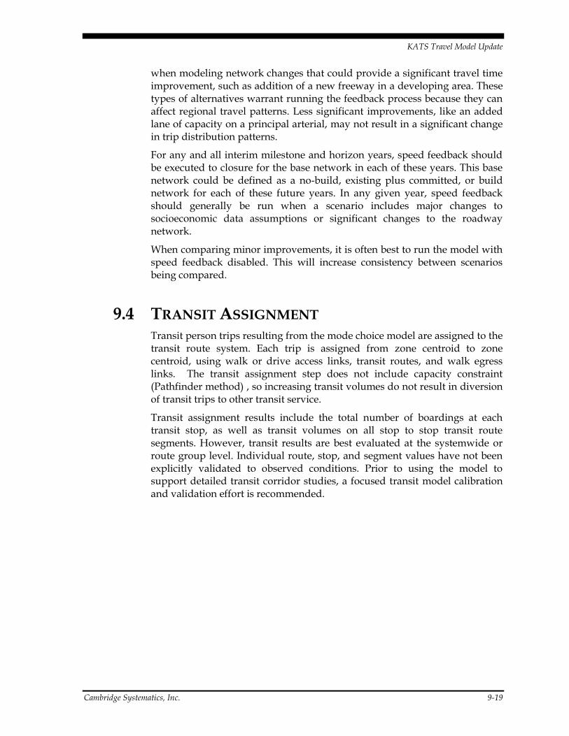
KATS Travel Model Update
Cambridge Systematics, Inc. 9-19
when modeling network changes that could provide a significant travel time improvement, such as addition of a new freeway in a developing area. These types of alternatives warrant running the feedback process because they can affect regional travel patterns. Less significant improvements, like an added lane of capacity on a principal arterial, may not result in a significant change in trip distribution patterns.
For any and all interim milestone and horizon years, speed feedback should be executed to closure for the base network in each of these years. This base network could be defined as a no-build, existing plus committed, or build network for each of these future years. In any given year, speed feedback should generally be run when a scenario includes major changes to socioeconomic data assumptions or significant changes to the roadway network.
When comparing minor improvements, it is often best to run the model with speed feedback disabled. This will increase consistency between scenarios being compared.
9.4 TRANSIT ASSIGNMENT Transit person trips resulting from the mode choice model are assigned to the transit route system. Each trip is assigned from zone centroid to zone centroid, using walk or drive access links, transit routes, and walk egress links. The transit assignment step does not include capacity constraint (Pathfinder method) , so increasing transit volumes do not result in diversion of transit trips to other transit service.
Transit assignment results include the total number of boardings at each transit stop, as well as transit volumes on all stop to stop transit route segments. However, transit results are best evaluated at the systemwide or route group level. Individual route, stop, and segment values have not been explicitly validated to observed conditions. Prior to using the model to support detailed transit corridor studies, a focused transit model calibration and validation effort is recommended.

KATS Travel Model Update
10-22 Cambridge Systematics, Inc.
10.0 Model Validation
This chapter describes the process and results of the calibration and validation of the 2010 KATS Model update. This includes specific comparison tests and statistical evaluations for the roadway, transit, and non-motorized modes. Because the model update reflects a 2010 base year, comparisons to observed traffic count and transit boarding data reflect 2010 conditions. Guidelines provided in the Travel Model Validation and Reasonableness Checking Manual, 2nd Edition (Travel Model Improvement Program, 2010) were followed in the validation of the KATS model.
The roadway system receives the most scrutiny in the process because it represents the largest amount of local travel and the highest public investment. Next is the transit system, which has a low relative share of trips but still represents a significant public investment. The non-motorized travel modes, simplified in the KATS model as bicycle and pedestrian modes, typically receive the lowest level of calibration and validation because they are particularly difficult to model using a TAZ-based aggregate travel model.
Ideally, the a travel model is calibrated and validated at every level of computation, including the traditional four steps of trip generation, trip distribution, mode choice, and trip assignment. For the KATS model, sufficient data were not available to independently calibrate the trip generation model. Chapter 7 of this report provides information about calibration and validation of the trip distribution model steps. This final chapter focuses on validation of the model generated traffic volumes and transit boardings to observed data, and also includes mode choice calibration results.
10.1 TRAFFIC ASSIGNMENT VALIDATION Roadway volumes resulting from traffic assignment were compared against traffic count data. This process, called traffic assignment validation, ensures that the model is reasonably representing observed traffic patterns. Traffic counts were obtained from various sources and placed on the roadway network. Travel model results were then compared to traffic count data using a variety of techniques, including regional comparisons, screenline comparisons, and visual inspection of individual links.
Overall Activity Level
Overall vehicle trip activity was validated by comparing count data to model results on all links where count data is available using two statistics: the Model Volume as compared to Count Volume and the Model VMT as compared to Count VMT. These statistics were reviewed at the facility type, area type, and regional level and are shown in Table 10.1.

KATS Travel Model Update
Cambridge Systematics, Inc. 10-23
Table 10.1 Regional Activity Validation
Category Number of
Counts Model Volume / Count Volume
Model VMT / Count VMT
VMT Target (variance from 100%)
Interstate/Freeway 36 102.5% 101.5% +/- 6%
Expressway 3 100.2% 99.3% +/- 6%
Principal Arterial 144 98.9% 95.3% +/- 7%
Minor Arterial 244 97.5% 95.1% +/- 10%
Collector 147 88.7% 88.8% +/- 20%
Minor Collector 14 96.7% 99.3% +/- 20%
CBD 13 96.7% 101.2% n/a
Urban 116 106.2% 102.7% n/a
Suburban 350 95.5% 96.9% n/a
Rural 173 103.8% 99.8% n/a
Systemwide 652 97.3% 97.4% +/- 5%
Note: Targets reflect MDOT validation criteria published in the MDOT Urban Model Improvement Program, Traffic Assignment document.
Screenlines
Another important validation test is the comparison of modeled volumes and observed traffic counts on screenlines. Screenlines are imaginary lines that extend across a series of roadway links and form a logical basis for evaluating regional travel movements in the model. Screenlines can also be drawn to separate major activity areas, along highways, or natural features. Results of the screenline analysis are listed in Table 10.2 and shown in Figure 10.1 along with a recommended maximum acceptable error for each screenline and cordon. A map of screenlines used in the KATS Model is shown in

KATS Travel Model Update
10-22 Cambridge Systematics, Inc.
Figure 10.2. The maximum acceptable error is based on guidance contained in the National Cooperative Highway Research Program (NCHRP) report number 25514, and reiterated in Chapter 4 of NCHRP report number 76515.
Table 10.2 Screenline Volumes and Counts
ID Screenline Description Model Volume Count Volume % Error
1 Kalamazoo North 98,907 95,286 4%
2 Kalamazoo South 61,559 57,449 7%
3 Kalamazoo West 190,099 177,973 7%
4 Kalamazoo East 104,233 98,533 6%
5 CBD Cordon 210,879 207,802 1%
6 Kalamazoo / Van Buren 82,549 76,462 8%
7 Kalamazoo / Portage 253,341 253,274 0.0%
Figure 10.1 Screenline Analysis
14 NCHRP Report No. 255, Highway Traffic Data for Urbanized Area Project Planning and Design (Transportation Research Board, National Research Council, December 1982).
15 NCHRP Report No. 765, Analytical Travel Forecasting Approaches for Project-Level Planning and Design (Transportation Research Board, 2014).

KATS Travel Model Update
Cambridge Systematics, Inc. 10-23
Figure 10.2 Screenlines

KATS Travel Model Update
10-24 Cambridge Systematics, Inc.
Measures of Error
While the model should accurately represent the overall level of activity, it is also important to verify that the model has an acceptably low level of error on individual links. It is expected that the model will not perfectly reproduce count volumes on every link, but the level of error should be monitored. The plot shown in Figure 10.3 demonstrates the ability of the Model to match individual traffic count data points. Table 10.3 lists percent root mean square error (% 𝑅𝑀𝑆𝐸) values and target values for each facility type and area type. General guidelines suggest that % 𝑅𝑀𝑆𝐸 should be below 40% region-wide, with values at or below 30% for high volume facility types. The % 𝑅𝑀𝑆𝐸 measure tends to over-represent errors on low volume facilities, so values on collector facilities are not particularly meaningful. Table 10.4 shows % RMSE values by volume group.
Figure 10.3 Count / Volume Comparison

KATS Travel Model Update
Cambridge Systematics, Inc. 10-25
Table 10.3 Root Mean Square Error by Facility Type and Area Type
Category Number of Counts RMSE % RMSE
Interstate/Freeway 36 3,244 14%
Expressway 3 1,445 12%
Principal Arterial 139 4,535 25%
Minor Arterial 244 2,869 36%
CBD 13 3,720 37%
Urban 116 2,926 29%
Suburban 345 3,544 33%
Rural 173 1,549 30%
Freeway / Arterial Total 422 3,408 27%
Overall 647 2,924 32%
Table 10.4 Root Mean Square Error by Volume Group
Volume Group RMSE % RMSE Target
0 - 5,000 1,729 66% < 100%
5,001 - 10,000 2,405 34% < 75%
10,001 - 15,000 3,290 26% < 50%
15,001 - 20,000 4,914 28% < 30%
20,001 - 30,000 4,572 19% < 30%
30,001 + 5,386 16% < 30%
Note: Targets reflect example validation targets published in the MDOT Urban Model Improvement Program, Traffic Assignment document.
10.2 TRANSIT ASSIGNMENT VALIDATION Transit assignment validation was performed first at a systemwide level, and then at a route group level. Systemwide transit validation ensures that the overall number of transit boardings is reasonably consistent with the number of observed boardings on an average school season weekday. Route group validation also compares modeled boardings to observed boardings, but considers groups of routes that serve a similar geographic area or market.
Systemwide Transit Assignment Validation
Systemwide transit validation requires a calibrated mode choice model that reflects a modeled number of trips that is consistent with observed data. Kalamazoo Transit reported a total of 7,341 average daily trips, with an average

KATS Travel Model Update
10-26 Cambridge Systematics, Inc.
of 1.45 transfers per trip. This equates to a total of 10,644 transit boardings on an average weekday. The calibrated model reasonably reflects these values as shown in Table 10.5.
The calibrated model reflects a slightly lower transfer rate that suggested by the observed data. To achieve this value, it was necessary to eliminate transfer penalties and implement a 5-minute transfer wait time for transfers occurring at the downtown Kalamazoo transfer center. Furthermore, the transfer wait time coefficient was reduced below the general out of vehicle wait time coefficient to increase the transfer rate seen in initial calibration attempts. Because the observed number of transfers per trip number is approximate, the mode choice and transit networks were not further adjusted beyond these reasonable levels to achieve a modeled value of 1.45.
Table 10.5 Systemwide Transit Validation Results
Observed Model Difference % Difference
Total Trips 7,341 7,314 -27 -0.4%
Total Boardings 10,644 10,312 -332 -3.1%
Average Boardings per Trip 1.45 1.41 0.04 -2.8%
Source: Boarding and transfer data provided by Kalamazoo Transit
Route Group Validation
Route group validation was performed for five distinct sets of routes, each serving a different geographic area. Route groups are defined in Table 10.6 and shown in Figure 10.4. The resulting validation by route group, shown in Figure 10.5, demonstrates that the mode choice and transit assignment model reasonably represent transit activity in the Kalamazoo area.
Table 10.6 Route Group Definitions
Route Group Name Included Transit Lines
North 6, 7, 15
East 5, 9, 10
South 1, 2, 8, 12, 13
Portage 26, 27, 28
West 3, 4, 11, 14, 16, 17, 18, 21, 22, 24
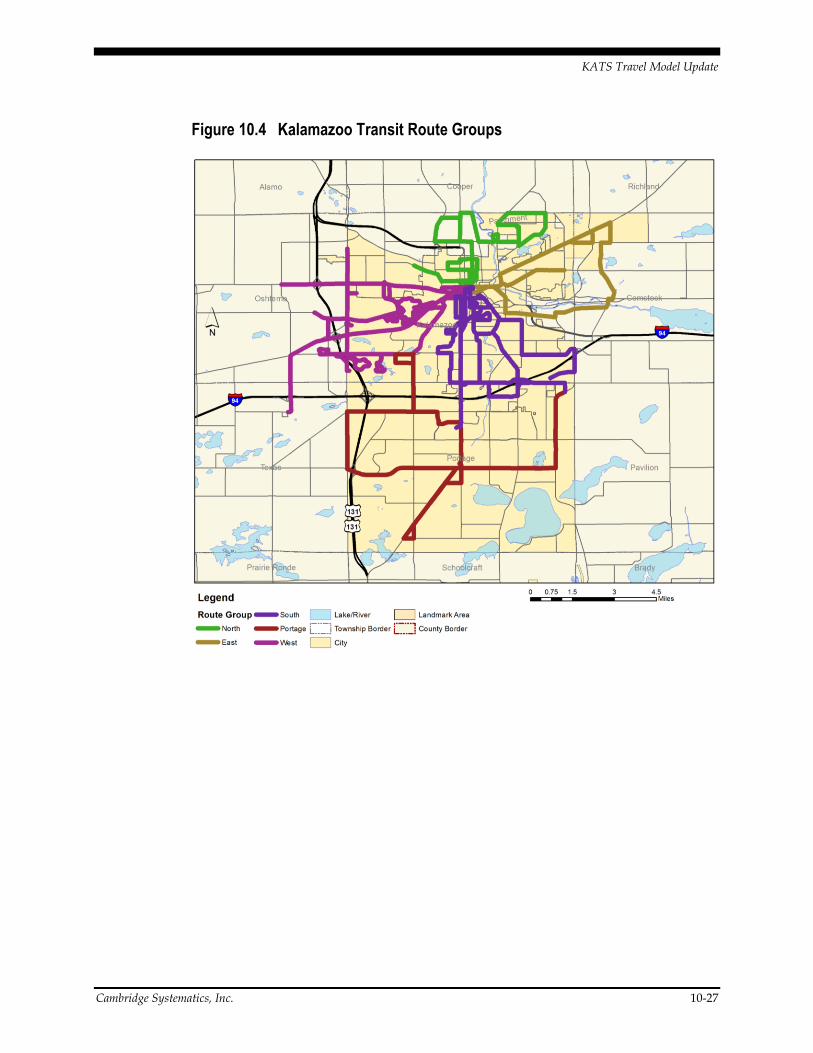
KATS Travel Model Update
Cambridge Systematics, Inc. 10-27
Figure 10.4 Kalamazoo Transit Route Groups

KATS Travel Model Update
10-28 Cambridge Systematics, Inc.
Figure 10.5 Transit Assignment Validation by Route Group
10.3 SENSITIVITY TESTS The base year validation measures described above are critical in ensuring the validity of the model. These measures show that the model adequately reproduces observed trip generation, distribution, mode split, and assignment patterns. However, the base year validation measures are static – they do not demonstrate the sensitivity of the model. This section describes a sensitivity testing process in which the model is run through a series of simple tests. These tests show that the model provides appropriate sensitivity to variables that are important in the forecasting and planning process.
Socioeconomic Data Adjustments
The addition of new land use data to a TAZ is expected to affect the total number of trips made, and the regional total VMT and VHT. The type and location of new land use data may impact the type of change seen. For example, addition of new land use data in the rural fringe areas surrounding the suburban area would be expected to result in higher VMT increases than addition of data in a developed urban area (e.g., infill development).
W
P
S
E
N
R² = 0.97530
1,000
2,000
3,000
4,000
5,000
6,000
0 1,000 2,000 3,000 4,000 5,000 6,000
Modele
d B
oard
ings
Observed Boardings

KATS Travel Model Update
Cambridge Systematics, Inc. 10-29
Isolated Changes
Land use sensitivity tests were performed in two TAZs – numbered 1720 (urban area near downtown Kalamazoo) and 919 (suburban area southwest of the I-94 / US 131 interchange) – shown in Figure 10.6. Household values were varied by increasing and decreasing totals by 1, 10, and 100 for each test zone. These tests showed a consistent number of trips per household added for each TAZ, but the rural TAZ generates a larger number of trips due to higher average household size, workers per household, and median income as shown in Table 10.7 and Table 10.8. VMT and VHT changes were generally consistent, but there were some variations. Variations were most noticeable on a per-household basis with a very small (1 or 10 household) change. This suggests that the model is sufficiently sensitive when testing changes to socioeconomic data, but caution should be used when testing extremely small changes.
Figure 10.6 Sensitivity Test Zones

KATS Travel Model Update
10-30 Cambridge Systematics, Inc.
Table 10.7 TAZ Based Sensitivity Tests
TAZ
HH Adjustment
Trip Change /
HH
VMT Change / HH
Trip Change
VMT Change VHT Change
n/a Baseline 13.3 n/a n/a n/a n/a
TAZ 1720 Urban Area
+1 10.3 12.0 10.3 12.0 -11.1
+10 10.4 18.3 104.1 183.0 4.1
+100 10.4 21.3 1036.0 2131.6 83.7
-1 10.3 45.6 10.3 45.6 3.4
-10 10.4 27.7 104.1 277.3 9.0
-100 10.4 21.3 1036.1 2127.7 88.0
TAZ 919 Suburban Area
+1 14.0 71.4 14.0 71.4 -0.6
+10 13.8 58.9 138.4 588.8 28.0
+100 13.8 60.9 1384.4 6092.4 219.1
-1 14.0 63.8 14.0 63.8 7.2
-10 13.8 65.9 138.4 659.4 18.3
-100 13.8 60.9 1384.5 6088.1 228.4
Note: These sensitivity tests were run with speed feedback disabled and with traffic assignment
convergence set to 10−5.
Table 10.8 Base Year Sensitivity Test Household Data
TAZ 2010
Households Average
Household Size
Average Workers per Household
Median Household
Income
1720 (urban) 155 1.75 0.79 19,524
919 (rural) 329 3.26 1.24 84,049
Wholesale Changes
In addition to verifying the model’s ability to react to small changes, it is necessary to ensure that the model can produce reasonable long-term forecast volumes. Table 10.9 represents the results of model runs for the forecast year 2045 using draft existing plus committed (E+C) forecast roadway networks. These results show reasonable sensitivity for predicting future conditions.
A review of model results shows that trip and VMT patterns are reasonable. Due to decreasing household size, the number of trips per household decreases slightly while the number of trips per person in the region increases slightly. VMT follows a similar pattern when considered on a per household and per person basis.

KATS Travel Model Update
Cambridge Systematics, Inc. 10-31
Table 10.9 Forecast Year Sensitivity Test Results
Scenario Total
Households Trips per
Household VMT per
Household Trips per Person
VMT per person
VMT per Trip
Base 2010 114,684 13.3 68.5 5.2 27.1 5.2
Forecast 2045 140,122 13.2 67.6 5.5 28.3 5.1
Notes: These sensitivity tests were run with speed feedback enabled and with traffic assignment
convergence set to 10−5. Results for 2045 reflect a test run and may not be consistent with the E+C or 2045 transportation plan model results.
Link Removal
This sensitivity test involves removing a link from the roadway network and observing the resulting change in traffic volumes. Two links were removed independently and the model results were evaluated for reasonableness. One test involved removing a moderately traveled link in the urban area, which was expected to have significant and intuitive impacts on network volumes. A second test involved removing a lightly traveled rural road, which was expected to have minimal impact on roadway volumes.
Table 10.10 shows the impacts of these changes on regional statistics, while Figure 10.7 shows the impact of removing an urban link with relatively high traffic volumes. The VMT statistics suggest that the model is relatively stable with respect to overall VMT and VHT numbers. Volume changes at the link level resulting from the removal of a heavily traveled urban link show intuitive and stable results.
Removing a lightly traveled local street produced very minor and intuitive changes to the traffic volumes in the immediate vicinity of the link. However, unrelated changes of up to 200 daily vehicles were observed elsewhere in the
roadway network with a traffic assignment convergence gap setting of 10−5. With a convergence setting of 10−6, unrelated network changes were isolated and did not exceed 60 daily vehicles. Results of this test are shown in Figure 10.8. While increasing the convergence setting to 10−7 further reduced such changes, the higher convergence resulted in significantly longer model run times. Due to
these observations, the default convergence limit has been increased from 10−5 to 10−6.
Table 10.10 Network Change Sensitivity Test Results
Scenario Total VMT % VMT Change Total VHT % VHT Change
Base 2010 7,853,006 n/a 207,247 n/a
Remove Urban Link 7,853,486 0.0061% 207,483 0.1141%
Remove Rural Link 7,853,275 0.0034% 207,244 -0.0015%
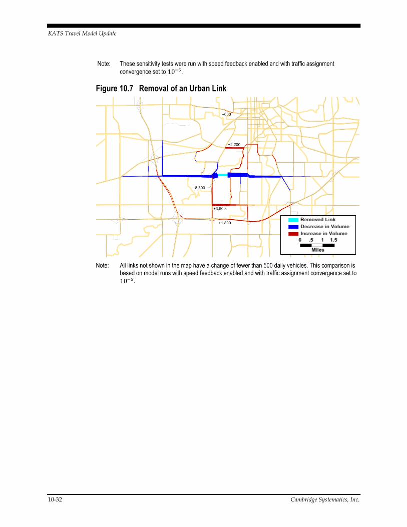
KATS Travel Model Update
10-32 Cambridge Systematics, Inc.
Note: These sensitivity tests were run with speed feedback enabled and with traffic assignment
convergence set to 10−5.
Figure 10.7 Removal of an Urban Link
Note: All links not shown in the map have a change of fewer than 500 daily vehicles. This comparison is based on model runs with speed feedback enabled and with traffic assignment convergence set to
10−5.

KATS Travel Model Update
Cambridge Systematics, Inc. 10-33
Figure 10.8 Removal of a Lightly Traveled Rural Link
Note: All links not shown in the map have a change of fewer than 15 daily vehicles. This comparison is based on model runs with speed feedback disabled and with traffic assignment convergence set to 10−6.


ÆaStadium Oakland
Whi
tes
Cork
Kilg
ore
Milh
amPortage
Kalam
azoo
Park
view
Mille
r Portage
Oakland
Westnedge
B.L. I-94
Pate
rson
North
Gull (M
-43) East Main
Alam
o
Crossto
wn
Burdick
Bronson
Burdick
Meije
r
Cros
sroa
dsMa
ll
Porta
geAd
ult E
d
° °
° ° °
° °
Wes
t Ma i
n
Howa
rd
Wes
t Mi
chiga
n
WMU
KendallSolon W
est
Mich
igan
A
B
C
I-94
I-94
US-131
Mich
igan
Love
llOregon
Idah
o
ParkRose
Rout
e 1 -
Wes
tned
geMo
nday
- Sa
turd
ayto
dow
ntow
nfro
m d
ownt
own
5:55 a
m6:0
56:1
56:3
06:4
57:0
07:1
57:3
07:3
57:4
58:0
08:0
58:1
58:3
08:4
59:0
09:1
59:3
09:4
510
:0010
:1510
:3010
:4511
:0011
:1511
:3011
:4512
:0012
:1512
:3012
:451:0
01:1
51:3
01:4
52:0
02:1
52:3
02:4
53:0
03:1
53:3
03:4
54:0
04:1
54:3
04:4
55:0
05:1
55:3
05:4
56:0
06:1
56:3
07:1
57:3
08:1
58:3
09:1
59:3
0AB
Meije
rs
Æa6:1
06:4
07:1
07:4
08:1
08:4
09:1
09:4
010
:1010
:4011
:1011
:4012
:1012
:401:1
01:4
02:1
02:4
03:1
03:4
04:1
04:4
05:1
05:4
06:1
06:4
07:4
08:4
09:4
0
6:20
6:42
7:12
7:42
8:12
8:42
9:12
9:42
10:12
10:42
11:12
11:42
12:12
12:42
1:12
1:42
2:12
2:42
3:12
3:42
4:12
4:42
5:12
5:42
6:12
6:42
7:12
8:12
9:12
10:12
6:50
7:20
7:50
8:20
8:50
9:20
9:50
10:20
10:50
11:20
11:50
12:20
12:50
1:20
1:50
2:20
2:50
3:20
3:50
4:20
4:50
5:20
5:50
6:20
6:50
7:50
8:50
9:50
Meije
rsAr
rives
Burd
ick, B
ay 11
Leav
esBu
rdick
, Bay
11C
APo
rtage
Adult
Ed.
Leav
esCr
ossro
ads
Æa
Visit
our w
eb si
te at:
www.
kmet
ro.co
m
ÆaLe
gend
Down
town
Tran
sfer P
oint
To D
ownto
wnFr
om D
ownto
wn
N
Bus d
oes n
ot se
rvice
area
.
Æa

Æa
BurdickNo
rth
Patte
rson
Westnedge
Portage
Mille
r
Milh
am
Kilg
ore
Cork
°
° °
°
°°
°
°
iSprinkle
Was
hing
ton
Sq.
Apar
tmen
ts
iMi
lwoo
d Ap
ts.k
Milw
ood
Elem
enta
ry
kWas
hing
ton
Elem
enta
ry
Meredith
I-94
Kilg
ore
Serv
ice R
oad
Kilg
ore
Portage
Portage
AMi
ller &
Porta
ge
°
°B
°De
vons
hire
Apar
tmen
ts
5:15
6:15
7:15
8:15
9:15
5:42
6:42
7:42
8:42
9:42
6:12
7:12
8:12
9:12
10:12
5:46
6:46
7:46
8:46
9:46
5:12
4:46
9:12
10:12
11:12
12:12
pm1:1
22:1
23:1
24:1
2
8:46
9:46
10:46
11:46
12:46
1:46
2:46
3:46
8:12
7:46
7:12
6:46
4:42
8:42
9:42
10:42
11:42
12:42
1:42
2:42
3:42
7:42
6:42
5:20
6:20
7:20
8:20
9:20
4:15
4:20
10:15
11:15
12:15
1:15
2:15
3:15
10:20
11:20
12:20
1:20
2:20
3:20
Arriv
esRo
se, B
ay 4
Porta
ge&
Mille
r
Mond
ay -
Satu
rday
to d
ownt
own
N
Visit
our w
eb si
te at:
www.
kmet
ro.co
m
ÆaLe
gend
Kalam
azoo
Tran
spor
tatio
nCe
nter
To D
ownt
own
From
Dow
ntow
n
Lim
ited
Serv
ice
Rout
e 2 -
Porta
geDe
vons
hire
Apar
tmen
ts BÆa
AÆa
Porta
ge&
Mille
r
8:20
9:20
7:20
6:20A
Leav
esRo
se, B
ay 4
8:15
9:15
7:15
6:15 a
mÆa
from
dow
ntow
n
Bron
son
Hosp
ital
°
Waln
ut
Mich
igan
°
PortageB.L. I-9
4
RosePark
°
°
°
Mich
igan
Love
ll
Park
RoseBurdick W
alnut John
Vine
Cros
stown
Portage
Dutto
nl
°ÆaEn
large
dDo
wnto
wn V
iew
Bron
son
Hosp
ital

I-94Drake
WestnedgeMose
lB.
L. U
S-13
1
Stad
ium
Wes
t Main
Park
view
Whi
tesBr
onso
n
SolonKendall
Wes
t Mich
igan
On-O
ff Ram
pC
Cam
pus
Load
ing
Zone
B
C
E
D
°
°
°
°
°
°No
rth
Douglas
°
US-131 US-131
°"KL"
OaklandHo
ward
Nichols
Alam
o
WMU
A
F °
11th
°°
°
°
°°
Wes
tMa
inMa
ll
Mapl
eHi
llMa
ll
The P
oint
Apar
tmen
ts
Villa
geAp
artm
ents
Wes
tland
Mead
ows
BA
BC
D6:0
0am
6:30
7:00
7:30
8:00
8:30
9:00
9:20
9:23
10:00
9:30
9:40
9:10
9:30
9:40
9:50
10:05
9:55
10:08
10:30
10:00
10:20
10:23
11:00
10:30
10:40
11:08
11:30
11:23
12:00
11:30
11:40
12:08
12:30
12:23
1:00
12:30
12:40
1:08
1:30
1:23
2:00
1:30
1:40
2:08
2:30
2:23
3:00
2:30
3:08
3:30
3:23
4:08
4:23
5:08
5:23
6:08
6:23
7:08
4:00
4:30
5:00
5:30
6:00
6:30
7:00
7:30
3:30
4:30
5:30
6:30
4:40
5:40
6:40
10:10
10:30
10:40
10:50
11:05
10:55
11:00
11:20
11:10
11:30
11:40
11:50
12:05
pm11
:5512
:0012
:2012
:1012
:3012
:4012
:501:0
512
:551:0
01:2
01:1
01:3
01:4
01:5
02:0
51:5
5
3:00
3:30
4:00
4:30
5:00
5:30
6:00
6:30
3:40
3:50
4:40
5:40
6:40
4:50
5:50
6:50
3:20
4:05
4:20
5:05
5:20
6:05
6:20
7:05
3:10
3:55
4:10
4:55
5:10
5:55
6:10
6:55
2:00
2:20
2:10
2:30
2:40
2:50
3:05
2:55
7:40
7:50
8:40
8:50
6:40
6:50
7:05
7:20
8:05
8:20
9:05
6:20
6:23
7:08
7:23
8:08
8:23
9:08
6:40
7:30
8:00
8:30
9:00
9:30
7:00
7:30
7:40
8:30
8:40
6:30
6:55
7:10
7:55
8:10
8:55
6:10
AC
FAr
rives
Camp
us
Load
ing Zo
neVil
lage
Apart
ments
The P
oint
Apart
ments
Wes
t Main
Mall
ELe
aves
Camp
us
Load
ing Zo
neMa
ple H
illMa
llTh
e Poin
t
Apart
ments
Villag
e
Apart
ments
Wes
tland
Mead
ows
Mond
ay -
Satu
rday
to W
MU L
oadi
ng Z
one
from
WMU
Loa
ding
Zon
e
N
Rout
e 3 -
Wes
t Mich
igan
Visit
our w
eb si
te at:
www.
kmet
ro.co
m
Lege
ndTo
WMU
Loa
ding
Zon
eFr
om W
MU L
oadi
ng Z
one
Bus d
oes n
ot se
rvice
area
.
9:08
9:00
9:20
9:10
9:23
10:00
9:30
9:40
10:08
10:20
9:30
9:40
9:50
10:05
9:55
9:30
8:30
8:40
8:50
9:05
8:55
7:23
7:30
7:40
7:50
8:05
7:55
8:08
8:30
8:23
9:00
8:30
8:40
8:00
8:20
8:10
8:00
7:30
7:40
7:00
7:20
7:10
3:40
2:40

Æa
Park
view
Bronson
Wes
t Mich
igan
Burdick
Westnedge
Portage
Mille
r
Cork
Milh
am
Portage
Sprinkle
ParkRose
KendallSolon
Stad
ium
Drake
°
°W
est M
ain
B.L. I-94
Pate
rson
North
Kalam
azoo
Howa
rd
Whi
tes
WMU
°
°°°°
° °
°
°
B
Greenleaf
Sprin
gmon
t
US-131
Kilg
ore
I-94
Michikal
Mich
igan
°Madison
° Sprin
gmon
t&
Madi
son
°
Rose
wood
Com
plex
12th
Oakland
°
°
°CEver
gree
nSo
uth
Crys
tal
Barnard
DA
Park
view
Hills
EPa
rkvie
w&
Barn
ard
Rout
e 4 -
Oakla
ndMo
nday
- Sa
turd
ay
Visit
our w
eb si
te at:
www.
kmet
ro.co
m
ÆaLe
gend
Kalam
azoo
Tran
spor
tatio
nCe
nter
To D
ownt
own
From
Dow
ntow
n
N
1:15
1:25
1:30
1:42
3:42
4:42
5:42
6:42
7:42
8:42
9:42
6:42
7:42
8:42
9:42
10:42
11:42
12:42
2:42
6:50
7:12
7:50
8:12
8:50
9:12
9:50
10:12
10:50
11:12
11:50
12:12
pm
12:50
1:12
1:50
2:12
3:50
4:12
4:50
5:12
5:50
6:12
6:50
7:12
7:50
8:12
8:50
9:12
9:50
10:12
2:50
3:12
3:15
3:25
3:30
4:15
4:25
4:30
5:15
5:25
5:30
6:15
6:25
6:30
7:15
7:25
7:30
8:15
8:25
8:30
9:15
9:25
9:30
6:15 a
m6:2
56:3
0
7:15
7:25
7:30
8:15
8:25
8:30
9:15
9:25
9:30
10:15
10:25
10:30
11:15
11:25
11:30
12:15
12:25
12:30
2:15
2:25
2:30
1:35
3:35
4:35
5:35
6:35
7:35
8:35
9:35
6:35
7:35
8:35
9:35
10:35
11:35
12:35
2:35
ÆaA
Leav
esRo
se, B
ay 2
Sprin
gmon
t
& Ma
dison
Park
view
Hills
Ever
gree
nSo
uth
BC
ÆaArriv
esRo
se, B
ay 2
Park
view
& Ba
rnar
d
E
to d
ownt
own
from
dow
ntow
n
Æ a
DRo
sewo
odCo
mplex

Gull (
M-43)
Pate
rson
Mount Olivet
Riverview
East
Main
m
°
°
° °
°
° °
Mose
l
Pate
rson
Stamford
Gertr
ude
Harrison
Mulh
earnNazareth
East
Main
Baker
Craft
Char
lesWashburn
Kenn
ilwor
th
Nazareth
Sprinkle
Charlotte
Mich
igan
B.L. I-94
North
Kalam
azoo Portage
Cros
stown
BurdickRosePark
°
°
Michiga
n
A
ÆaLe
aves
Burd
ick, B
ay 13
Arriv
esBu
rdick
, Bay
13Ea
stwo
odPl
aza
6:18 a
m6:2
56:4
26:4
56:5
57:1
27:1
57:2
57:4
27:4
57:5
58:1
28:1
58:2
58:4
28:4
58:5
59:1
29:1
59:2
59:4
29:4
59:5
510
:1210
:1510
:2510
:4210
:4510
:5511
:1211
:1511
:2511
:4211
:4511
:5512
:12 pm
12:15
12:25
12:42
12:45
12:55
1:12
1:15
1:25
1:42
1:45
1:55
2:12
2:15
2:25
2:42
2:45
2:55
3:12
3:15
3:25
3:42
3:45
3:55
4:12
4:15
4:25
4:42
4:45
4:55
5:12
5:15
5:25
5:42
5:45
5:55
6:12
6:15
6:25
6:42
6:45
6:55
7:12
7:15
7:25
7:42
7:45
7:55
8:12
8:15
8:25
8:42
8:45
8:55
9:12
9:15
9:25
9:42
9:45
9:55
10:12
Mond
ay -
Satu
rday
to d
ownt
own
from
dow
ntow
n
N
Visit
our w
eb si
te at:
www.
kmet
ro.co
m
ÆaLe
gend
Down
town
Tran
sfer
Poi
nt
To D
ownt
own
From
Dow
ntow
n
Æa
Rout
e 5 -
East
Main
Eastw
ood
Plaz
a
Naza
reth
Cente
rÆa
A

Wes
t Main
Haym
ac
and
G A
ÆJ
k
Kind
leber
ger
Park
Parc
hmen
tHi
gh S
choo
l
°°
°°
°
°
°
°°
°
°° ° ° °
Mose
l
Douglas
Burdick
Pitcher
Mose
lLi
nkRiverview
B.L.
I-94
Rivervie
w Glen
dale
RandomHaymac
Mount Olivet
"G" Gu
ll (M-43
)
East
Main
Cros
stown
Portage
Burdick
B.L. I-94
North
Kalam
azoo
Pate
rson
ParkRose
Westnedge
Hopk
ins
Edwards
Sout
h
Westnedge
"G"
°
°
°
VirginiaPark
Orient
Mount Olive
t
Rans
om
Ediso
n
G an
dW
estn
edge
CLi
nk
° °
°
°
B
Leav
esRo
se,
Bay 1
0G
and
Westn
edge
Arriv
esRo
se,
Bay 1
0G
and
Westn
edge
AÆa
2:25
2:42
3:55
4:55
5:55
6:55
7:55
8:55
9:55
4:12
5:12
6:12
7:12
8:12
9:12
10:02
7:25
7:42
8:25
8:42
9:25
9:42
10:25
10:42
11:25
11:42
12:25
12:42
1:25
1:42
2:55
3:12
6:45 a
m6:5
5
7:45
7:55
8:45
8:55
9:45
9:55
10:45
10:55
11:45
11:55
12:45
12:55
1:45
1:55
3:15
3:25
4:15
4:25
5:15
5:25
6:15
6:25
7:15
7:25
8:15
8:25
9:15
9:25
2:15
2:25
2:22
3:52
4:52
5:52
6:52
7:52
8:52
9:52
7:22
8:22
9:22
10:22
11:22
12:22 1:2
2
2:52
2:12
3:42
4:42
5:42
6:42
7:42
8:42
9:42
7:12
8:12
9:12
10:12
11:12
12:12
pm
1:12
2:42
Haym
ac&
"G" B
AÆa
Mond
ay -
Satu
rday
to d
ownt
own
from
dow
ntow
n
N
Rout
e 6 -
Parc
hmen
t
Visit
our w
eb si
te at:
www.
kmet
ro.co
mÆa
ÆaLe
gend
Kalam
azoo
Tran
spor
tatio
nCe
nter
To D
ownt
own
From
Dow
ntow
n
Link C

Æa
Westnedge
Park
RoseBurdick
Portage
Cros
stown
B - L I-9
4
Stadium
Oakland
Wes
t Mich
igan
Wes
t Main
North
Pate
rson
Riverview
Douglas
Alam
o
rMetro
Tra
nsit
°
°
°
°
° °
°
°
B.L.
US-
131
Mich
igan
Rans
om Kalam
azoo
°
°
BHi
llsid
eMi
ddle
Scho
ol
°North
wind
A
6:15 a
m6:4
57:1
57:4
58:1
58:4
59:1
59:4
510
:1510
:4511
:1511
:4512
:1512
:451:1
51:4
52:1
52:4
53:1
53:4
54:1
54:4
55:1
55:4
56:1
56:4
57:1
57:4
58:1
58:4
59:1
59:4
5
10:23
10:53
11:23
11:53
12:23
12:53
1:23
1:53
6:25
6:55
7:25
7:55
8:25
8:55
9:25
9:55
2:25
2:55
3:25
3:55
4:25
4:55
5:25
5:55
6:25
6:55
7:25
7:55
8:25
8:55
9:25
9:55
Hillside
Middle
Scho
ol
ÆaA
BLe
aves
Rose,
Bay 9
Arriv
es
Rose,
Bay 9
6:42
7:12
7:42
8:12
8:42
9:12
9:42
10:12
10:42
11:12
11:42
12:12
12:42
1:12
1:42
2:12
2:42
3:12
3:42
4:12
4:42
5:12
5:42
6:12
6:42
7:12
7:42
8:12
8:42
9:12
9:42
10:12
Æa
Mond
ay -
Satu
rday
to d
ownt
own
from
dow
ntow
nN
Rout
e 7 -
Alam
o
Visit
our w
eb si
te at:
www.
kmet
ro.co
m
ÆaLe
gend
Down
town
Tran
sfer
Poi
ntTo
Dow
ntow
nFr
om D
ownt
own
Æa
Northw
ind
10:25
10:55
11:25
11:55
12:25
12:55
1:25
1:55

Æa
Crossto
wn
Burdick
Westnege
Cork
Portage
Mille
rB.L.
I-94
Howa
rd
Sprinkle
26th
26th
Cork
Stoc
kbrid
ge
Covin
gton
Vanrick
Fulford
Cork
Whi
tes
Portage
Was
hing
ton
Squa
re A
pts.
°
ASt
ockb
ridge
& Fu
lford
Indu
stria
l
Fulfo
rd &
CorkkMi
lwoo
d Jr
.Hi
ghsc
hool
°
°°
°
°
°
°°
°
°
°° ° °
°
°B D
I-94
North
Kalam
azoo
ParkRose
Pate
rson
Kers
ten
Cour
t
Park
Circ
le
Pitcher
C
°
°
°
°
°
ÆaA
AÆa
Leav
esRo
se,
Bay 6
Stoc
kbrid
ge
& Fu
lford
Arriv
es
Rose
,Ba
y 6W
ashin
gton
Squa
reFu
lford
& Co
rkLe
aves
Indus
trial
N
Rout
e 8 -
Egles
ton
Mond
ay -
Satu
rday
to d
ownt
own
from
dow
ntow
n
BC
D6:1
76:2
26:4
27:1
0 +7:2
07:4
26:4
56:5
08:1
0 +8:2
08:4
27:4
57:5
09:1
0 #9:2
09:4
210
:10 +
10:20
10:30
10:42
11:10
11:20
11:30
11:42
12:10
pm#
12:20
12:30
12:42
1:10
1:20
1:30
1:42
2:10 +
2:20
2:30
2:42
3:10 *
#3:4
22:4
52:5
02:5
23:4
0 *+
4:12
4:40 *
+5:1
23:1
53:2
04:1
54:2
05:4
0 *+
6:12
5:15
5:20
6:40 +
6:50
7:12
7:40
7:50
8:12
8:40
8:50
9:12
9:40
9:50
10:12
6:15
6:22
7:15
7:22
8:15
8:22
9:15
9:22
* Bus
servi
ces M
ilwoo
d Midd
le Sc
hool
on th
is trip
whe
n sch
ool
is in
sess
ion.
+ Bu
s Ser
vices
Ker
sten C
ourt
- W
eekd
ays O
nly
8:45
8:50
9:45
9:50
10:45
10:50
10:52
11:45
11:50
11:52
12:45
12:50
12:52
1:45
1:50
1:52
5:55 a
m
Visit
our w
eb si
te at:
www.
kmet
ro.co
mÆaLe
gend
Kalam
azoo
Tran
spor
tatio
nCe
nter
To D
ownt
own
From
Dow
ntow
n
Lim
ited
Serv
ice
Æa
2:40 *
+3:1
22:1
52:2
02:2
2
Was
hingt
onSq
uare
# Bus
servi
ces M
RC on
26th
Stre
et.
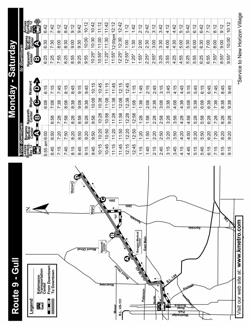
Æa
Mose
l
Gull (M
-43)
East
Main
Sprinkle
26th
Sprinkle
Portage
Crossto
wn
WestnedgeParkRose
BurdickNorth
Mount Olivet
26th
Borg
ess M
edica
lCe
nter
Naza
reth
Cent
er
°
°
°
°
°
°
°
°
°
°
A"H
"B
B.L.
US-
131 Pa
ters
on
RiverviewMount O
livet
B.L. I-94
Wes
t Mich
igan
I-94
C
°
°
°
DW
almar
t
Meije
r
Walm
art
6:08
7:08
7:38
8:08
8:38
9:08
9:38
10:08
10:38
11:08
11:38
12:08
12:38
1:08
1:38
2:08
2:38
3:08
3:38
4:08
4:38
5:08
5:38
6:08
6:38
7:38
8:38
9:38
6:15
7:15
7:45
8:15
8:45
9:15
9:45
10:15
10:45
11:15
11:45
12:15
12:45
1:15
1:45
2:15
2:45
3:15
3:45
4:15
4:45
5:15
5:45
6:15
6:45
7:45
8:45
9:45
Leav
esBu
rdick
,Ba
y 12
Naza
reth
Cent
erAÆaAr
rives
Burd
ick,
Bay 1
2Bo
rges
sMe
dica
lCe
nter
Naza
reth
Cent
er B 6:25
6:30
6:42
7:25
7:30
7:42
7:55
8:00
8:12
8:25
8:30
8:42
8:55
9:00
9:12
9:25
9:30
9:42
9:55
10:00
10:12
10:25
*10
:3010
:4210
:55*
11:00
11:12
11:25
*11
:3011
:4211
:55*
12:12
12:25
*12
:3012
:4212
:55*
1:00
1:12
1:25*
1:30
1:42
1:55*
2:00
2:12
2:25*
2:30
2:42
2:55*
3:00
3:12
3:25
3:30
3:42
3:55
4:00
4:12
4:25
4:30
4:42
4:55
5:00
5:12
5:25
5:30
5:42
5:55
6:00
6:12
6:25
6:30
6:42
6:55
7:00
7:12
7:55*
8:00
8:12
8:55*
9:00
9:12
9:55*
10:00
10:12
12:00
pm
NRo
ute 9
- Gu
llMo
nday
- Sa
turd
ayto
dow
ntow
nfro
m d
ownt
own
5:55 a
m6:4
56:5
06:5
87:1
57:2
07:2
87:4
57:5
07:5
88:1
58:2
08:2
88:4
58:5
08:5
89:1
59:2
09:2
89:4
59:5
09:5
810
:1510
:2010
:2810
:4510
:5010
:5811
:1511
:2011
:2811
:4511
:5011
:5812
:1512
:2012
:2812
:4512
:5012
:581:1
51:2
01:2
81:4
51:5
01:5
82:1
52:2
02:2
82:4
52:5
02:5
83:1
53:2
03:2
83:4
53:5
03:5
84:1
54:2
04:2
84:4
54:5
04:5
85:1
55:2
05:2
85:4
55:5
05:5
86:1
56:2
06:2
87:1
57:2
07:2
88:1
58:2
08:2
89:1
59:2
09:2
8
Visit
our w
eb si
te at:
www.
kmet
ro.co
m
ÆaLe
gend
Kalam
azoo
Tran
spor
tatio
nCe
nter
To D
ownt
own
From
Dow
ntow
n
Æa
*Ser
vice t
o New
Hor
izon V
illage
ÆaBo
rges
sMe
dica
lCe
nter
6:00A
BCMe
ijer
D
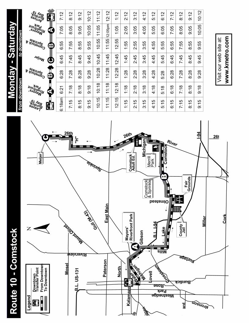
Æa Love
ll
lI-9
4
Mills
Wes
t Mich
igan
East
Main
Gull (M
-43)
Mount Olive
t
Riverview
Wes
t Main
Alamo
Kalam
azoo
North
Pate
rson
26th
Cork
Mille
r
River
Meije
r
Com
stoc
kAd
ult E
d.
Fair
Grou
nds
Coun
tyJa
il
C
°
°
°
°
°
°°
°
°
°
°
°
°
ÆI
k ÆJ
"H"
Lake
26th 26th
Crossto
wn
Bronson
RosePark
Howa
rd
Westnedge
Oakland
Burdick
Portage
B.L.
I-94
Sprinkle
Mose
l
B.L.
US-
131
°
°
B
Gibs
onWate
r
Michiga
nMa
yors
'Ri
verfr
ont P
ark
A
°
°
°
°OlmsteadCo
mstoc
k&
Sprin
kleMe
rrill
Park Co
mst
ock
Mich
igan
BÆa
CA
6:45
6:55
7:12
8:12
9:12
10:12
11:12
10:05
11:05
1:12
2:12
3:12
4:12
5:12
6:12
7:12
8:12
9:12
10:12
7:45
7:55
8:45
8:55
9:45
9:55
10:45
11:45
12:45
10:55
11:55
12:55
1:45
1:55
2:45
2:55
3:45
3:55
4:45
4:55
5:45
5:55
6:45
6:55
7:45
7:55
8:45
8:55
9:45
9:55
6:18a
m
7:15
8:15
9:15
11:15
12:15
1:15
2:15
3:15
4:15
5:15
6:15
7:15
8:15
9:15
10:15
6:21
7:18
8:18
9:18
10:18
11:18
12:18
1:18
2:18
3:18
4:18
5:18
6:18
7:18
8:18
9:18
6:28
7:28
8:28
9:28
10:28
11:28
12:28
1:28
2:28
3:28
4:28
5:28
6:28
7:28
8:28
9:28
ÆaB
A
Leaves Burdick, Bay 19
Meijer
Comstock & Sprinkle
Arrives Burdick, Bay 19
Comstock & Sprinkle
Mond
ay -
Satu
rday
to d
ownt
own
from
dow
ntow
n Visit
our w
eb si
te at:
www.
kmet
ro.co
mMayors' Riverfront Park
7:05
8:05
9:05
1:05
2:05
3:05
4:05
5:05
6:05
7:05
8:05
9:05
10:05Mayors' Riverfront Park
12:05
pm12
:12
Rout
e 10 -
Com
stoc
k NÆa
Lege
ndDo
wnto
wnTr
ansf
er P
oint
To D
ownt
own
From
Dow
ntow
n
B
Æa

Æa
WMU
Wes
t Mich
igan
Wes
t Main
Park
view
OaklandOakland
Westnedge
Burdick
Crossto
wn
ParkRose
North
Pate
rson
Kalam
azoo
East
Main
B.L. I-94
Cork
Kilg
ore
Howa
rdSolon
9th
Drake
Mille
r
Bronson
Kendall
Alamo k
°°
°
°
°
°
°
°
A
"KL"
US-131
I-94
Wes
t Mich
igan
Kilg
ore
°
Stad
ium
Love
ll
Western
Mich
igan
Stad
ium
Dr.
Apts
.
°
Stad
ium
& 11
th
BKV
CC°
Elm
Vall
ey
Æa 7:12
8:12
9:12
10:12
11:12
12:12 pm 1:12
2:12
3:12
4:12
5:12
6:12
7:12
8:12
9:12
10:12Arriv
es
Rose, Bay
1
B
7:46
8:46
9:46
10:46
11:46 12:46
1:46
2:46
3:46
4:46
5:46
6:46
7:46
8:46
9:46Leav
es KVCC
6:46
ÆaA
B6:1
5am
7:15
7:40
8:40
6:40
8:15
9:15
9:22
9:40
10:15
10:22
10:40
11:15
11:22
11:40
12:15
12:22
12:40
1:15
1:22
1:40
2:15
2:22
2:40
3:15
3:22
3:40
4:15
4:40
5:40
6:40
7:40
8:40
9:40
5:15
6:15
7:15
8:15
9:15Leav
es
Rose, Bay
1 Stadium
& 11th
Arrives KVCC
NRo
ute 1
1 - S
tadi
um/K
VCC
to d
ownt
own
from
dow
ntow
n
ÆaDo
wnto
wnTr
ansf
er P
oint
To D
ownt
own
From
Dow
ntow
n
Lege
nd
Mond
ay -
Satu
rday
Bus d
oes n
ot se
rvice
area
.
Visit
our w
eb si
te at:
www.
kmet
ro.co
m
Æa7:2
2
8:22
6:22
4:22
5:22
6:22
7:22
8:22
9:22
Æa 6:50
7:50
8:50
9:50
10:50
11:50
12:50
1:50
2:50
3:50
4:50
5:50
6:50
7:50
8:50
9:50
Stadium
& 11th

WMU
Milh
am
Oakland
Westnedge
Burdick
Mille
r
Cork
Sprinkle
SprinkleMilh
am
Kilg
ore
Howa
rd
Kendall
Wes
t Main
North Ka
lamaz
oo
B.L.
I-94
Crossto
wnWestnedge
Whi
tes
Alamo
Portage
Portage
Gull (
M-43)
Pate
rson
Oakland
ParkRose
Meije
r
jjjCa
ndlew
yck A
pts.
Duke
Airp
ort
YMCA
°°
°
° °
°
°
°
°°
A°
I-94Stad
ium
I-94
B
Bron
son
Hosp
ital
mC
Peele
r
Mapl
eWaln
utDu
tton
Vine
John
RoseFo
rest
Oak
Sout
hElea
nor
Bron
son
o°
°
Loy N
orrix
High
Sch
ool
Mich
igan
ÆaA
Leav
esBu
rdick
,Ba
y 20
Meije
rYM
CAB 7:0
08:0
0
9:00
10:00
11:00
1:00
2:00
3:30
3:40
3:15
3:20
3:55
4:30
5:30
6:30
7:30
8:30
9:30
4:40
5:40
6:40
7:40
8:40
9:40
4:15
4:20
5:15
5:20
6:15
6:20
7:15
7:20
8:15
8:20
9:15
9:20
4:55
5:55
6:55
7:55
8:55
9:55
12:00 pm
6:45
am6:5
07:1
0
8:10
9:10
10:10
11:10
12:10
1:10
2:10
7:45
7:50
8:45
8:50
9:45
9:50
10:45
10:50
11:45
11:50
12:45
12:50
1:45
1:50
7:25
8:25
9:25
10:25
11:25
12:25
1:25
2:25
N
Rout
e 12 -
Bro
nson
Mond
ay -
Satu
rday
to d
ownt
own
from
dow
ntow
n
ÆaDo
wnto
wnTr
ansf
er P
oint
To D
ownt
own
From
Dow
ntow
n
Lege
nd
Visit
our w
eb si
te at:
www.
kmet
ro.co
m
Bus d
oes n
ot se
rvice
area
.
Æa
2:30
2:40
2:15
2:20
2:55
Airp
ort
AYM
CA
C
4:12
5:12
6:12
7:12
8:12
9:12
10:12ÆaArriv
esBu
rdick
,Ba
y 20
7:42
8:42
9:42
10:42
11:42
12:42
1:42
2:42
3:12

Æa
Whi
tes
Kilg
ore
Cork
Mille
r
Portage
Howa
rd
Oakland
Wes
t Mich
igan
Wes
t Main
Sprinkle
WestnedgePark
Westnedge
Rose
Cros
stow
n
WMU
Stadium
BurdickKalam
azoo
North
East
Main
B.L. I-94
D
Rose
Kilg
ore
Portage
Stoc
k brid
ge
Bank
Bron
son MR
C
Meije
r
Bron
son
FIA
iHi
lltop
Apts
.
iCa
ndlew
yck A
pts.
A B
I-94
Portage
lll
°
°
° ° °
°°°
°
°
°
°
° °
Lake
Jasper
VineLo
vell
BurdickBurdick
CGo
odwi
ll
Waln
ut
John Dutto
n
Alco
tt
6:27
6:42
7:25
7:55
8:25
8:55
9:25
9:55
10:25
10:55
11:25
12:25
12:55
1:25
1:55
2:25
2:55
3:25
3:55
4:25
4:55
5:25
5:55
6:25
6:55
7:55
8:55
9:55
11:55
7:27
7:42
7:57
8:12
8:27
8:42
8:57
9:12
9:27
9:42
9:57
10:12
10:27
10:42
10:57
11:12
11:27
11:42
11:57
12:12
pm12
:2712
:4212
:571:1
21:2
71:4
21:5
72:1
22:2
72:4
22:5
73:1
23:2
73:4
23:5
74:1
24:2
74:4
24:5
75:1
25:2
75:4
25:5
76:1
26:2
76:4
26:5
77:1
27:5
78:1
28:5
79:1
29:5
710
:12
ÆaA
Leav
esRo
se, B
ay 7
MRC
FIA
Meije
rGo
odwi
ll
CB
D Saturday Service
6:00a
m6:4
56:4
96:5
16:5
57:1
07:1
57:1
97:2
17:2
57:4
07:4
57:4
97:5
17:5
58:1
08:1
58:1
98:2
18:2
58:4
08:4
58:4
98:5
18:5
59:1
09:1
59:1
99:2
19:2
59:4
09:4
59:4
99:5
19:5
510
:1010
:1510
:1910
:2110
:2510
:4010
:4510
:4910
:5110
:5511
:1011
:1511
:1911
:2111
:2511
:4011
:4511
:4911
:5111
:5512
:1012
:1512
:1912
:2112
:2512
:4012
:4512
:4912
:5112
:551:1
01:1
51:1
91:2
11:2
51:4
01:4
51:4
91:5
11:5
52:1
02:1
52:1
92:2
12:2
52:4
02:4
52:4
92:5
12:5
53:1
03:1
53:1
93:2
13:2
53:4
03:4
53:4
93:5
13:5
54:1
04:1
54:1
94:2
14:2
54:4
04:4
54:4
94:5
14:5
55:1
05:1
55:1
95:2
15:2
55:4
05:4
55:4
95:5
15:5
56:1
06:1
56:1
96:2
16:2
56:4
07:1
57:1
97:2
17:2
57:4
08:1
58:1
98:2
18:2
58:4
09:1
59:1
99:2
19:2
59:4
0
6:10
AÆaAr
rives
Rose
, Bay
7B
MRC
FIA
N
Rout
e 13 -
Sou
th B
urdi
ckMo
nday
- Sa
turd
ayto
dow
ntow
nfro
m d
ownt
own
ÆaDo
wnto
wnTr
ansf
er P
oint
To D
ownt
own
From
Dow
ntow
n
Lege
nd
Bus d
oes n
ot se
rvice
area
.Vi
sit ou
r web
site
at:ww
w.km
etro
.com
Æa
7:13
7:43
8:13
8:43
9:13
9:43
10:13
10:43
11:13
12:13
12:43
1:13
1:43
2:13
2:43
3:13
3:43
4:13
4:43
5:13
5:43
6:13
6:43
7:43
8:43
9:43
11:43
Good
will
C

Æa
WMU
Park
view
Stad
ium
Wes
t Mich
igan
9th
Drake
NicholsAl
amo
DrakeB.L.
US-131
Mose
l
Douglas Pate
rson
North
Oakland
Howa
rd
Kilg
ore
Oakland
Westnedge
Burdick
ParkRose Burdick
RiverviewMount O
livet
Gull (
M-43)
East
Main
Bronson
Cork
Whi
tes
9th9th
KL
PortageSolon
KendallA
°
°
°
°
°
°
°
US-131
US-131
BerkleyKa
lamaz
ooW
est M
ainC
B
DE
Frien
dship
Villa
ge
Kalam
azoo
Centr
al Hi
ghSc
hool
Maple
Hill M
allTr
ansfe
rPo
int
Ever
gree
nNo
rthMe
ijer
°
° °
6:30
6:32
7:00
7:02
7:30
7:32
8:00
8:02
8:30
8:32
9:00
9:02
9:30
9:32
10:00
10:02
10:30
10:32
11:00
11:02
11:30
11:32
12:02
12:30
12:32
1:00
1:02
1:30
1:32
2:00
2:02
2:30
2:32
3:00
3:02
3:30
3:32
4:00
4:02
4:30
4:32
5:00
5:02
5:30
5:32
6:00
6:02
6:30
6:32
7:30
7:32
9:45
8:45
7:45
9:30
9:32
9:15
9:35
9:38
8:30
8:32
8:15
8:35
8:38
7:15
7:35
7:38
9:55
8:55
7:55
10:12
9:12
8:12
12:00
6:45
7:15
7:45
8:15
8:45
9:15
9:45
10:15
10:45
11:15
11:45
12:15
12:45
1:15
1:45
2:15
2:45
3:15
3:45
4:15
4:45
5:15
5:45
6:15
6:45
6:15a
m6:4
57:1
57:4
58:1
58:4
59:1
59:4
510
:1510
:4511
:1511
:4512
:1512
:451:1
51:4
52:1
52:4
53:1
53:4
54:1
54:4
55:1
55:4
56:1
5ÆaA
BLe
aves
Rose
,Ba
y 3Fri
ends
hip
Villag
eKa
lamaz
oo
Centr
al
ÆaE
6:35
6:38
7:05
7:08
7:35
7:38
8:05
8:08
8:35
8:38
9:05
9:08
9:35
9:38
10:05
10:08
10:35
10:38
11:05
11:08
11:35
11:38
12:08
12:35
12:38
1:05
1:08
1:35
1:38
2:05
2:08
2:35
2:38
3:05
3:08
3:35
3:38
4:05
4:08
4:35
4:38
5:05
5:08
5:35
5:38
6:05
6:08
6:35
6:38
12:05C
DMap
le Hil
l
MallEv
ergree
n
North
Meijer
6:55
7:25
7:55
8:25
8:55
9:25
9:55
10:25
10:55
11:25
11:55
12:25
12:55
1:25
1:55
2:25
2:55
3:25
3:55
4:25
4:55
5:25
5:55
6:25
6:55
7:12
7:42
8:12
8:42
9:12
9:42
10:12
10:42
11:12
11:42
12:12
pm12
:421:1
21:4
22:1
22:4
23:1
23:4
24:1
24:4
25:1
25:4
26:1
26:4
27:1
2
CMap
le Hil
l
Mall
Mond
ay -
Satu
rday
to d
ownt
own
from
dow
ntow
n
N
Rout
e 14 -
Wes
t Main
Visit
our w
eb si
te at:
www.
kmet
ro.co
m
ÆaDo
wnto
wnTr
ansf
er P
oint
To D
ownt
own
From
Dow
ntow
n
Lege
nd
Æa
Arriv
esRo
se,
Bay 3
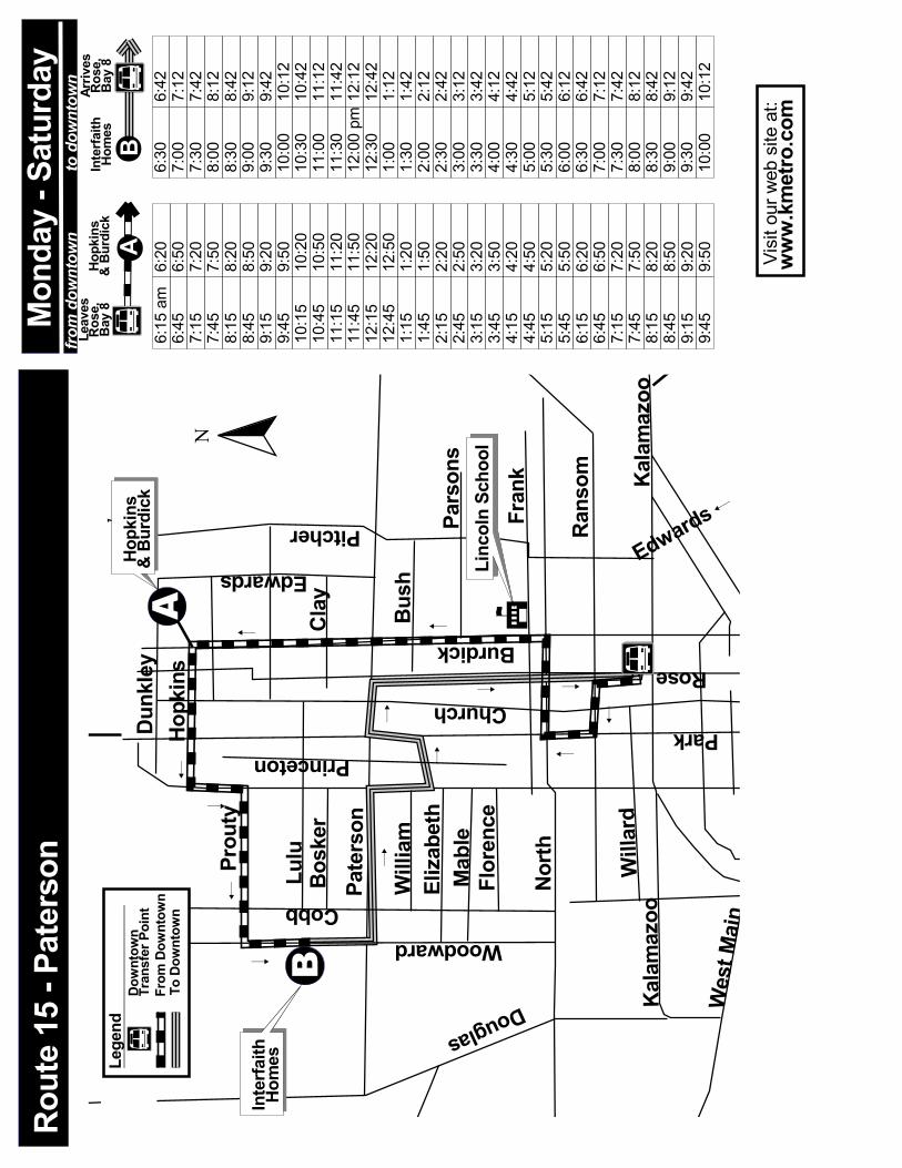
Æa
Pate
rson
Kalam
azoo
Wes
t Main
Wes
t Mich
igan
Westnedge
PortageKalam
azoo
Mount Olivet
Gull (M
-43)
Riverview
Oakland
Douglas
B
A
Linc
oln
Scho
ol
°°
°
°
°°
°
°
°
°
° °
°
Inte
rfaith
Hom
es
Hopk
ins
& Bu
rdick
kNo
rth
Flor
ence
Mabl
eEl
izabe
thW
illiam
Bosk
erLu
luCl
ay Bush
Pars
ons
Fran
k
Rans
om
Princeton
Church
Willa
rdEdwards
Pitcher
CobbWoodward
Dunk
ley
Prou
ty
Hopk
ins
Burdick
SouthEdwards
°
°
Park
Rose
ÆaB
6:30
6:42
7:00
7:12
7:30
7:42
8:00
8:12
8:30
8:42
9:00
9:12
9:30
9:42
10:00
10:12
10:30
10:42
11:00
11:12
11:30
11:42
12:00
pm12
:1212
:3012
:421:0
01:1
21:3
01:4
22:0
02:1
22:3
02:4
23:0
03:1
23:3
03:4
24:0
04:1
24:3
04:4
25:0
05:1
25:3
05:4
26:0
06:1
26:3
06:4
27:0
07:1
27:3
07:4
28:0
08:1
28:3
08:4
29:0
09:1
29:3
09:4
210
:0010
:12
ÆaA
Leav
esRo
se,
Bay 8
Arriv
esRo
se,
Bay 8
Inte
rfaith
Hom
esHo
pkin
s&
Burd
ick
6:15 a
m6:2
06:4
56:5
07:1
57:2
07:4
57:5
08:1
58:2
08:4
58:5
09:1
59:2
09:4
59:5
010
:1510
:2010
:4510
:5011
:1511
:2011
:4511
:5012
:1512
:2012
:4512
:501:1
51:2
01:4
51:5
02:1
52:2
02:4
52:5
03:1
53:2
03:4
53:5
04:1
54:2
04:4
54:5
05:1
55:2
05:4
55:5
06:1
56:2
06:4
56:5
07:1
57:2
07:4
57:5
08:1
58:2
08:4
58:5
09:1
59:2
09:4
59:5
0
to d
ownt
own
N
Rout
e 15 -
Pat
erso
nMo
nday
- Sa
turd
ayfro
m d
ownt
own
ÆaDo
wnto
wnTr
ansf
er P
oint
To D
ownt
own
From
Dow
ntow
n
Lege
nd
Visit
our w
eb si
te at:
www.
kmet
ro.co
m
Æa

Æa
m
mm
ooo
Wes
t Main
Solon
Howa
rd
North
Alam
oNichols
C Vine Neighborhood
Valle
ys
Wald
oLib
rary
kBe
rnha
rd
l
Mille
r
South
&Oa
k Oak &
Love
ll Vine
A
°
°°
°
°
°
°
° °
°
°
°
°
Stud
ent R
ecre
ation
Cente
r
Kalam
azoo
Sout
hLo
vell
Love
ll
Ceda
r
°
Waln
utDu
tton
Olive
r Whe
aton
Kendall
LafayetteHoward
DavisMerrill
Oak
Westnedge
Park
RoseBurdick
Douglas
West M
ichiga
n
Wes
t Mich
igan
Stadium
Oakland
Crosstown
Portage
DormitoryGo
ldsw
orth
Rankin
Busin
ess
Cour
t
m Faun
ceWilb
ur
Camp
usLo
ading
Zone
B
Elea
nore
NA
BÆa
Oak & Love
llAr
rives
Campu
s
Load
ing Zo
ne
5:50 a
m5:5
25:5
76:1
56:1
76:2
76:4
56:4
76:5
77:1
57:1
77:2
77:4
57:4
77:5
78:1
58:1
78:2
78:4
58:4
78:5
79:1
59:1
79:2
79:4
59:4
79:5
710
:1510
:1710
:2710
:4510
:4710
:5711
:1511
:1711
:2711
:4511
:4711
:5712
:1512
:1712
:2712
:4512
:4712
:571:1
51:1
71:2
71:4
51:4
71:5
72:1
52:1
72:2
72:4
52:4
72:5
73:1
53:1
73:2
73:4
53:4
73:5
74:1
54:1
74:2
74:4
54:4
74:5
75:1
55:1
75:2
75:4
55:4
75:5
76:1
56:1
76:2
76:4
56:4
76:5
77:1
57:1
77:2
77:4
57:4
77:5
78:1
58:1
78:2
78:4
58:4
78:5
79:1
59:1
79:2
79:4
59:4
79:5
7
BC
Æa
Mond
ay -
Satu
rday
to d
ownt
own
from
dow
ntow
n
South
&Oa
kLe
aves
Campu
s
Load
ing Zo
ne
Rout
e 16 -
Lov
ell
6:30
6:36
6:42
7:00
7:06
7:12
7:30
7:36
7:42
8:00
8:06
8:12
8:30
8:36
8:42
9:00
9:06
9:12
9:30
9:36
9:42
10:00
10:06
10:12
10:30
10:36
10:42
11:00
11:06
11:12
11:30
11:36
11:42
12:00
pm12
:0612
:1212
:3012
:3612
:421:0
01:0
61:1
21:3
01:3
61:4
22:0
02:0
62:1
22:3
02:3
62:4
23:0
03:0
63:1
23:3
03:3
63:4
24:0
04:0
64:1
24:3
04:3
64:4
25:0
05:0
65:1
25:3
05:3
65:4
26:0
06:0
66:1
26:3
06:3
66:4
27:0
07:0
67:1
27:3
07:3
67:4
28:0
08:0
68:1
28:3
08:3
68:4
29:0
09:0
69:1
29:3
09:3
69:4
210
:00
ÆaDo
wnto
wnTr
ansf
er P
oint
To D
ownt
own
From
Dow
ntow
n
Lege
nd
Bus d
oes n
ot se
rvice
area
.
Leav
esRo
se,
Bay 5
Arriv
esRo
se,
Bay 5
Æa
6:00
6:06
6:12
Visit
our w
eb si
te at:
www.
kmet
ro.co
m

Leav
es
Campu
s
Load
ing Zo
ne
AC
BD
Waldo
Lawso
n
EBern
hard Va
lleys
8:10
8:40
9:10
9:40
10:10
10:40
11:10
11:40
12:10
12:40
1:10
1:40
2:10
2:40
3:10
3:40
4:10
4:40
5:10
5:40
6:10
6:40
7:10
7:40
8:10
8:40
9:10
7:40
7:35
8:05
8:35
9:05
9:35
10:05
10:35
11:05
11:35
12:05
12:35
1:05
1:35
2:05
2:35
3:05
3:35
4:05
4:35
5:05
5:35
6:05
6:35
7:05
7:35
8:05
8:35
9:05
7:55
7:58
8:00
8:25
8:28
8:30
8:55
8:58
9:00
9:25
9:28
9:30
9:55
9:58
10:00
10:25
10:28
10:30
10:55
10:58
11:00
11:25
11:28
11:30
11:55
11:58
12:00
12:25
12:28
12:30
12:55
12:58
1:00
1:25
1:28
1:30
1:55
1:58
2:00
2:25
2:28
2:30
2:55
2:58
3:00
3:25
3:28
3:30
3:55
3:58
4:00
4:25
4:28
4:30
4:55
4:58
5:00
5:25
5:28
5:30
5:55
5:58
6:00
6:25
6:28
6:30
6:55
6:58
7:00
7:25
7:28
7:30
7:55
7:58
8:00
8:25
8:28
8:30
8:55
8:58
9:00
7:28
7:25
7:30
8:25
8:55
9:25
9:55
10:25
10:55
11:25
11:55
12:25
12:55
1:25
1:55
2:25
2:55
3:25
3:55
4:25
4:55
5:25
5:55
6:25
6:55
7:25
7:55
8:25
8:55
9:25
7:55A
Arriv
es
Campu
s
Load
ing Zo
neLe
aves
Campu
s
Load
ing Zo
neAr
rives
Campu
s
Load
ing Zo
ne
AC
BD
Bernha
rd
Valle
ys
EWald
oLa
wson
8:05
8:35
9:05
9:35
10:05
10:35
11:05
11:35
12:05
12:35
1:05
1:35
2:05
2:35
3:05
3:35
4:05
4:35
5:05
5:35
6:05
6:35
7:05
7:35
8:05
8:35
9:05
9:35
7:35
7:32
8:02
8:32
9:02
9:32
10:02
10:32
11:02
11:32
12:02
12:32
1:02
1:32
2:02
2:32
3:02
3:32
4:02
4:32
5:02
5:32
6:02
6:32
7:02
7:32
8:02
8:32
9:02
9:32
7:45
7:50
8:00
8:15
8:20
8:30
8:45
8:50
9:00
9:15
9:20
9:30
9:45
9:50
10:00
10:15
10:20
10:30
10:45
10:50
11:00
11:15
11:20
11:30
11:45
11:50
12:00
12:15
12:20
12:30
12:45
12:50
1:00
1:15
1:20
1:30
1:45
1:50
2:00
2:15
2:20
2:30
2:45
2:50
3:00
3:15
3:20
3:30
3:45
3:50
4:00
4:15
4:20
4:30
4:45
4:50
5:00
5:15
5:20
5:30
5:45
5:50
6:00
6:15
6:20
6:30
6:45
6:50
7:00
7:15
7:20
7:30
7:45
7:50
8:00
8:15
8:20
8:30
8:45
8:50
9:00
9:15
9:20
9:30
7:20
7:15
7:30
8:15
8:45
9:15
9:45
10:15
10:45
11:15
11:45
12:15
12:45
1:15
1:45
2:15
2:45
3:15
3:45
4:15
4:45
5:15
5:45
6:15
6:45
7:15
7:45
8:15
8:45
9:15
9:45
7:45A
lk
o
m
m
m D
C
B
Mille
r
Bern
hard
Ellsw
orth
Hall St
uden
t Rec
reat
ion
Cent
er
Valle
y 1
Wald
oLi
brar
y
Knollw
ood
Kendall
Howard
Wes
t Mich
igan
Howa
rd
Oakland
West
Mich
igan
Olive
r
Stadium
Lafayette
Dormitory
Gilkison
Wilb
ur
Rankin
Gold
swor
th
GreenwoodCam
pus
Load
ing
Zone
Am
Sang
ren
°
°°
°°Business Court E
Laws
on
°
°
°°
°
°
°
°
°
°°
°
°
°
° °
°
°°
NMo
nday
-Frid
ay O
nly
Fall/S
prin
g Se
mes
ters
Whe
n W
MU is
in S
essio
n
Rout
e 17 -
Gol
d Ca
mpu
sMo
nday
- Fr
iday
www.
kmet
ro.co
mVi
sit o
ur w
ebsit
e at
Circ
le B-
-trav
els so
uth
out o
fth
e cam
pus l
oadi
ng zo
ne, o
r co
unte
r-clo
ckwi
se ar
ound
cam
pus.
Lege
ndCi
rcle
A--tr
avels
nor
th o
ut o
fth
e cam
pus l
oadi
ng zo
ne, o
r clo
ckwi
se ar
ound
cam
pus.
Circ
le A
Circ
le B

oo
Vine Neighborhood
o
East
Cam
pus
CHHS
°
°
°
Kendall
Howard
Wes
t Mich
igan
Howa
rd
Oakland
West
Mich
igan
Love
ll
Whe
aton
DavisMerrill
Olive
r
Kalam
azoo
Douglas
Ceda
r
Waln
utDu
tton
Vine
Lafayette
OakSout
h
Love
ll
Wes
t Main
Valle
ys
Stadium
Wester
n
Greenwood
E
F°
°
°
°
°
°
Cam
pus
Load
ing
Zone
B
BCSt
adiu
m D
r.Ap
artm
ents
CCa
mpu
sLo
adin
gZo
ne
°
°F
E
C
Wester
n Stadium
Mille
r
LafayetteHoward
mWes
ternB Ha
ys
Arca
dia
Vandegiessen
StadiumBe
rnha
rd
Wald
o m
ml
Knollwood
°
°BA
Arriv
esCa
mpus
Load
ing Zo
ne
AA
Leav
esCa
mpus
Load
ing Zo
neSt
adium
Dr.
Apart
ments
Mond
ay -
Frid
ayto
WMU
Cam
pus
from
WMU
Cam
pus
B7:1
5am
7:45
8:15
8:45
9:15
9:45
10:15
10:45
11:15
11:45
12:15
12:45
1:15
1:45
2:15
2:45
3:15
3:45
4:15
4:45
6:15*
6:45*
7:15*
7:45*
8:15*
8:45*
9:15*
5:45
5:15
7:17
7:47
8:17
8:47
9:17
9:47
10:17
10:47
11:17
11:47
12:17
12:47
1:17
1:47
2:17
2:47
3:17
3:47
4:17
4:47
6:17*
6:47*
7:17*
7:47*
8:17*
8:47*
9:17*
5:47
5:17
7:30
8:00
8:30
9:00
9:30
10:00
10:30
11:00
11:30
12:00
12:30
1:00
1:30
2:00
2:30
3:00
3:30
4:00
4:30
5:00
6:30*
7:00*
7:30*
8:00*
8:30*
9:00*
9:30*
6:00
5:30
7:30
8:00
8:30
9:00
9:30
10:00
10:30
11:00
11:30
12:00
12:30
1:00
1:30
2:00
2:30
3:00
3:30
4:00
4:30
5:00
6:30*
7:00*
7:30*
8:00*
8:30*
9:00*
9:30*
6:00*
5:30
CEa
st Ca
mpus
CHHS
*Ser
vice p
rovid
ed M
onda
y th
roug
h Thu
rsday
only.
Rout
e 18 -
How
ard
To C
ampu
s Loa
ding
Zon
eFr
om C
ampu
s Loa
ding
Zon
eLe
gend
Visit
our w
eb si
te at:
www.
kmet
ro.co
m
Mond
ay-F
riday
Onl
yFa
ll/Spr
ing
Sem
este
rsW
hen
WMU
is in
Ses
sion
N
9:45*

lk
o
m m
mm
Vine Neighborhood
oi
i
i
° °
°
°
°
°
°°
BLafayette
Stadium
Douglas
Kalam
azoo
North
Alam
o
Olive
r
MerrillDavis
Whe
aton
Love
ll
West
Mich
igan
Oakland
Howa
rd
Howard
Kendall
SolonNichols
Kend
allMa
nor
The L
andi
ng
Cam
pus
Load
ing
Zone
oEl
lswor
th H
all
Bern
hard
Stud
ent R
ecCe
nter
Valle
ys Wald
o
Mille
r
Wes
t Main
Greenwood
Knollwood
Wes
t Mich
igan
Howa
rdVa
lley Bu
sines
s A
°
Solo
n &
Wes
t Main
Whi
teha
ll
°
°
°
AA
Leav
esCa
mpu
sLo
adin
g Zo
neAr
rives
Cam
pus
Load
ing
Zone
Solo
n &
Wes
t Main
to C
ampu
sfro
m C
ampu
s
B
Rout
e 21 -
Sol
on-K
enda
ll
7:45
7:49
8:15
8:19
8:45
8:49
9:15
9:19
9:45
9:49
10:15
10:19
10:45
10:49
11:15
11:19
11:45
11:49
12:15
12:19
12:45
12:49
1:15
1:19
1:45
1:49
2:15
2:19
2:45
2:49
3:15
3:19
3:45
3:49
4:15
4:19
4:45
4:49
5:15
5:19
5:45
5:49
6:15*
6:19*
6:55*
6:49*
7:15*
7:19*
7:45*
7:49*
8:15*
8:19*
8:45*
8:49*
9:15*
9:19*
8:00*
8:30*
9:00*
9:30*
8:00
8:30
9:00
9:30
10:00
10:30
11:00
11:30
12:00
pm12
:301:0
01:3
02:0
02:3
03:0
03:3
04:0
04:3
05:0
05:3
06:0
06:3
0*7:0
0*7:3
0*
7:15 a
m7:1
97:3
0
NÆa
Down
town
Tran
sfer
Poi
nt
To C
ampu
sFr
om C
ampu
s
Lege
nd
Mond
ay -
Frid
ay
Visit
our w
eb si
te at:
www.
kmet
ro.co
m
Mond
ay-F
riday
Onl
yFa
ll/Spr
ing
Sem
este
rsW
hen
WMU
is in
Ses
sion

lk
Solon
Kendall
Howard
Wes
t Mich
igan
Howa
rd
Oakland
West
Mich
igan
Love
ll
Douglas
Nichols
Stadium
Lafayette
Wes
t Main
oo
m m
Stud
ent R
ecre
atio
nCe
nter
m
oVa
lleys
Ellsw
orth
Hall
Bern
hard
Mille
r
Wald
o
Cam
pus
Load
ing
Zone Kn
ollw
ood
Apts
.
Greenwood
Knollwood
Fraternity Village
California
°
°
° °
°
°
°
°
°
°
°
°
°
°
°
°
RankinABu
sines
s
B
Rout
e 22 -
Laf
ayet
te
7:42
8:12
8:42
9:12
9:42
10:12
10:42
11:12
11:42
12:12
12:42
1:12
1:42
2:12
2:42
3:12
3:42
4:12
4:42
5:12
5:42
6:12
6:42*
7:12*
7:42*
8:12*
8:42*
9:12*
5:30
5:34
6:00
6:04
6:30*
6:34*
7:00*
7:04*
7:30*
7:34*
8:00*
8:04*
8:30*
8:34*
9:00*
9:04*
7:30
7:34
8:00
8:04
8:30
8:34
9:00
9:04
9:30
9:34
10:00
10:04
10:30
10:34
11:00
11:04
11:30
11:34
12:00
pm12
:0412
:3012
:341:0
01:0
41:3
01:3
42:0
02:0
42:3
02:3
43:0
03:0
43:3
03:3
44:0
04:0
44:3
04:3
45:0
05:0
4
7:00 a
m7:0
47:1
2A
ALe
aves
Cam
pus
Load
ing
Zone
Arriv
esCa
mpu
sLo
adin
g Zo
neKn
ollw
ood
Apar
tmen
tsB
Mond
ay -
Frid
ayto
Cam
pus
from
Cam
pus
N
ÆaDo
wnto
wnTr
ansf
er P
oint
To C
ampu
sFr
om C
ampu
s
Lege
nd
Visit
our w
eb si
te at:
www.
kmet
ro.co
m
Mond
ay-F
riday
Onl
yFa
ll/Spr
ing
Sem
este
rsW
hen
WMU
is in
Ses
sion

Stud
ent R
ecre
atio
nCe
nter
lk
Crossto
wn
oo
m
mVine Neighborhood
o
East
Cam
pus
CHHS
°
°
°
°
Howard
Wes
t Mich
igan
Howa
rd
Oakland
West
Mich
igan
Love
ll
Whe
aton
DavisMerrill
Olive
r
Ceda
r
Waln
ut
Dutto
n
Vine
Park
Rose
Burdick
Crosstown
Westnedge
Oak
Portage
Sout
h
Love
ll
Wald
o
Mille
r
Ellsw
orth
Hall
Valle
ys
Bern
hard
Stadium
Vandegiessen
Arca
diaHays
AC
B
Wester
n
°
°
°
° mEa
stCa
mpu
s
AB
7:30a
m
6:30
8:30
12:30
12:50
1:10
1:30
7:50
8:10
8:30
8:50
9:10
9:30
9:50
10:10
10:30
10:50
11:10
11:30
11:50
12:10
3:30
4:10
4:30
4:50
5:10
5:30
5:50
6:10
6:30
6:50
7:10
7:30
7:50
8:10
1:50
2:10
3:10
2:50
2:30
3:50
8:50
9:10
9:30
7:40
11:50
11:30
11:10
10:50
10:30
10:10
9:50
9:30
9:10
8:50
8:30
8:10
7:50
12:10
12:30
12:50
1:10
1:30
1:50
2:50
3:10
3:50
4:10
4:30
4:50
5:10
5:30
5:50
6:10
2:30
2:10
3:30
6:50
7:10
7:30
8:30
8:50
9:10
8:10
7:50
7:20
7:40
8:40
9:00
9:20
8:20
8:00
3:20
4:00
4:20
4:40
5:00
5:20
5:40
6:00
6:20
6:40
7:00
1:00
1:20
1:40
2:00
3:00
2:40
2:20
3:40
12:20
12:40
8:00
8:20
8:40
9:00
9:20
9:40
10:00
10:20
10:40
11:00
11:20
11:40
12:00
pm
ALe
aves
East
Cam
pus
CHHS
Arriv
esEa
st C
ampu
sCH
HSN
Rout
e 24 -
Eas
t Cam
pus S
ilver
Mond
ay -
Frid
ayto
Eas
t Cam
pus
from
Eas
t Cam
pus
To E
ast C
ampu
sFr
om E
ast C
ampu
sLe
gend
Mond
ay-F
riday
Onl
yFa
ll/Spr
ing
Sem
este
rsW
hen
WMU
is in
Ses
sion
Bern
hard
Visit
our w
eb si
te at:
www.
kmet
ro.co
m

Æa
WMU
Park
view
Stad
ium
Wes
t Mich
igan
DrakeNo
rth
OaklandHowa
rd
Kilg
ore
Oakland
Westnedge
Burdick
ParkRose
Burdick
Cork
Whi
tes
SolonKendall
°
US-131
Edwards
Wes
t Main
°°
°
°
°W
MU M
ainCa
mpus
°
°
°
C
A B Stad
ium&
Howa
rd
°Parkv
iewCa
mpus
Mond
ay -
Frid
ay
Sum
mer
I and
II25
- W
MU P
arkv
iew C
ampu
sfro
m W
MU ca
mpu
sto
WMU
cam
pus
From
Main
Cam
pus
To M
ain C
ampu
sLe
gend
Lim
ited
Serv
ice
Visit
our w
eb si
te at:
www.
kmet
ro.co
m
Mond
ay -
Frid
ay O
nly
Sum
mer
I and
II Se
mes
ters
Whe
n W
MU is
in S
essio
n.Bu
s sto
ps at
des
igna
ted
stop
s onl
y.
1:06
1:36
2:36
5:20
12:20
1:20
3:20
9:20
1:02
9:30
1:32
9:40
2:02
9:50
2:32
12:00
12:02
1:00
1:02
2:00
2:02
3:00
3:02
5:00
12:36
9:20
10:20
11:20
8:00
8:02
9:00
9:02
10:00
10:02
9:10
12:32
11:00
11:02
8:20
7:30
2:52
2:12
2:50
2:10
1:30
1:32
12:52
12:50
9:20
1:02
9:30
1:32
9:40
2:02
9:50
2:32
12:30
12:50
1:30
1:50
2:30
2:50
3:30
3:50
6:30
12:12
12:10
11:32
11:30
10:52
10:50
10:12
10:10
8:30
8:50
9:30
9:50
10:30
10:50
9:10
12:32
11:50
11:30
5:30
5:50
6:50
7:50
5:02
6:00
6:02
6:20
7:00
7:02
7:20
AB
CHo
ward
&St
adium
CA
Leav
esPa
rkvie
wCa
mpus
Arriv
esPa
rkvie
wCa
mpus
Leav
esW
MU M
ainCa
mpus
Arriv
esW
MU M
ainCa
mpus
N
Mondays and Wednesdays OnlyService ends at 4:50 on Tuesdays and Thursdays
Service ends at 3:50 on Fridays
2:20
4:00
4:02
4:20
4:30
4:50

Stad
ium
Kilg
ore
Oakland
Westnedge
BurdickBurdick
Cork
Whi
tes
US-131
I-94
°
Rom
ence
Cent
re
Currier
12th
Angling
M.L.
Kin
g Jr
.
Oakland
Constitution
Brow
n
Texa
s
US-131
Milha
mMe
adow
s
Porta
geCi
tyHa
llBo
rges
s at
Woo
dbrid
geHi
lls
Anna
'sVi
neya
rdD
Cros
sroad
sMa
llE °
°
°
°
°
° °
°
i
Sprin
gmon
tBarnardPa
rkvie
w
B
Parkv
iew&
Barn
ard
A
C
5:02
8:25
10:52
10:12
8:25
9:50
4:32
7:25
4:52
4:12
3:32
2:52
2:12
1:32
12:52
1:02
1:32
2:02
2:32
3:02
3:32
4:02
12:25
1:25
2:25
3:25
4:25
5:25
6:25
12:12
11:32
10:25
12:32
11:25
5:02
9:25
9:25
10:12
7:25
4:36
5:06
7:50
5:02
7:35
10:40
5:02
8:10
10:52
10:12
8:10
9:50
4:32
7:10
4:52
4:12
3:32
2:52
2:12
1:32
12:52
1:02
1:32
2:02
2:32
3:02
3:32
4:02
12:10
pm1:1
02:1
03:1
04:1
05:1
06:1
0
12:12
11:32
10:10
12:32
11:10
5:02
9:10
9:10
10:12
7:10
7:55
6:50
4:32
6:35
1:06
1:36
2:06
2:36
3:06
4:50
4:06
11:50
12:50
1:50
2:50
3:50
5:50
1:02
1:32
2:02
2:32
3:02
3:32
4:02
11:35
12:35
1:35
2:35
3:35
4:35
5:35
12:36
7:35
10:12
7:25
7:50
10:50
10:10
9:30
8:50
9:50
10:50
8:35
9:35
12:32
10:35
10:30
6:55
4:10
3:30
2:50
2:10
1:30
12:50
9:20
9:30
9:40
9:50
10:00
10:10
10:20
11:55
12:55
1:55
2:55
3:55
4:55
5:55
12:10
11:30
9:55
9:10
10:55
5:06
8:50
5:02
8:35
10:40
8:55
5:06
9:50
5:02
9:35
10:40
9:55
AB
CBo
rges
s at
Woo
dbrid
ge
DE
Milha
mMe
adow
sCr
ossr
oads
Mall
APo
rtage
City
Hall
Park
view
& Ba
rnar
dPo
rtage
City
Hall
6:50
7:55
10:10
6:55
8:55
5:02
7:25
10:52
9:50
4:32
6:25
4:52
4:12
3:32
2:52
2:12
1:32
12:52
1:02
1:32
2:02
2:32
3:02
3:32
4:02
11:25
12:25
1:25
2:25
3:25
4:25
5:25
12:12
11:32
9:25
12:32
10:25
5:02
8:25
5:02
9:25
8:25
To P
orta
ge C
ity H
allFr
om P
orta
ge C
ity H
allLe
gend
Lim
ited
Serv
ice
Mond
ay -
Satu
rday
26 -
Cent
re W
est
from
City
Hall
to C
ity H
all
Visit
our w
eb si
te at:
www.
kmet
ro.co
mN
6:35
10:12
6:25 a
m

Burdick
°
Brow
n
Cent
reMilh
am
Currier
SprinkleEx
ecut
ive
Corporate
Bish
op
Porta
geCi
ty Ha
llCe
ntre &
Sprin
kle
Portage
Com
mer
cial
°
°
°
° °
°
Meredith °
°Maple
Ridg
eAp
artm
ents
°
C°
°
°Ce
ntre &
Porta
ge °
DB
A
Mond
ay -
Satu
rday
27 -
Cent
re E
ast
from
City
Hall
to C
ity H
all
4:36
5:06
7:42
5:02
7:30
10:40
5:02
7:55
10:52
10:12
7:55
9:50
4:32
6:55
4:52
4:12
3:32
2:52
2:12
1:32
12:52
1:02
1:32
2:02
2:32
3:02
3:32
4:02
11:55
12:55
1:55
2:55
3:55
4:55
5:55
12:12
11:32
9:55
12:32
10:55
5:02
8:55
5:02
9:55
8:55
10:12
6:55
7:46
6:42
4:32
6:30
1:06
1:36
2:06
2:36
3:06
4:42
4:06
11:42
12:42
1:42
2:42
3:42
5:42
1:02
1:32
2:02
2:32
3:02
3:32
4:02
11:30
12:30
1:30
2:30
3:30
4:30
5:30
12:36
7:30
7:42
10:50
10:10
9:30
8:42
9:42
10:42
8:30
9:30
12:32
10:30
10:30
6:46
4:10
3:30
2:50
2:10
1:30
12:50
9:20
9:30
9:40
9:50
10:00
10:10
10:20
11:46
12:46
1:46
2:46
3:46
4:46
5:46
12:10
11:30
9:46
9:10
10:46
5:06
8:42
5:02
8:30
10:40
8:46
5:06
9:42
5:02
9:30
10:40
9:46
AB
CCe
ntre
&Sp
rinkle
DA
Cent
re &
Porta
gePo
rtage
City
Hall
Porta
geCi
ty Ha
llMa
ple R
idge
Apar
tmen
ts
6:42 a
m7:4
610
:106:4
6
8:46
5:02
7:25
10:52
10:12
7:25
9:50
4:32
6:25
4:52
4:12
3:32
2:52
2:12
1:32
12:52
1:02
1:32
2:02
2:32
3:02
3:32
4:02
11:25
12:25
1:25
2:25
3:25
4:25
5:25
12:12
11:32
9:25
12:32
10:25
5:02
8:25
5:02
9:25
8:25
To P
orta
ge C
ity H
allFr
om P
orta
ge C
ity H
allLe
gend
Lim
ited
Serv
ice
Visit
our w
eb si
te at:
www.
kmet
ro.co
m
N

Cent
re
Melo
dyWestnedge
Baco
n
Oste
rhou
t
Shaver
Oakland
Brow
n
CurrierPorta
geCi
ty Ha
ll
Wal-
Mart
Meije
r
The C
ross
ings
A
B C
D
°
°
°
°
°
°
°°
kPo
rtage
Centr
al
Mond
ay -
Satu
rday
28 -
Shav
erfro
m C
ity H
allto
City
Hall
5:02
8:15
10:52
10:12
8:15
9:50
4:32
7:15
4:52
4:12
3:32
2:52
2:12
1:32
12:52
1:02
1:32
2:02
2:32
3:02
3:32
4:02
12:15
1:15
2:15
3:15
4:15
5:15
6:15
12:12
11:32
10:15
12:32
11:15
5:02
9:15
9:15
10:12
7:15
5:02
10:15
4:36
5:06
8:04
5:02
7:58
10:40
5:02
8:12
10:52
10:12
8:12
9:50
4:32
7:12
4:52
4:12
3:32
2:52
2:12
1:32
12:52
1:02
1:32
2:02
2:32
3:02
3:32
4:02
12:12
1:12
2:12
3:12
4:12
5:12
6:12
12:12
11:32
10:12
12:32
11:12
5:02
9:12
5:02
10:12
9:12
10:12
7:12
8:08
7:04
4:32
6:58
1:06
1:36
2:06
2:36
3:06
5:04
4:06
12:04
pm1:0
42:0
43:0
44:0
4
6:04
1:02
1:32
2:02
2:32
3:02
3:32
4:02
11:58
12:58
1:58
2:58
3:58
4:58
5:58
12:36
7:58
10:12
7:55
8:04
10:50
10:10
9:30
9:04
10:04
11:04
8:58
9:58
12:32
10:58
10:30
7:08
4:10
3:30
2:50
2:10
1:30
12:50
9:20
9:30
9:40
9:50
10:00
10:10
10:20
12:08
1:08
2:08
3:08
4:08
5:08
6:08
12:10
11:30
10:08
9:10
11:08
5:06
9:04
5:02
8:58
10:40
9:08
5:06
10:04
5:02
9:58
10:40
10:08
7:04
8:08
10:10
7:08
9:08
5:02
7:55
10:52
9:50
4:32
6:55
4:52
4:12
3:32
2:52
2:12
1:32
12:52
1:02
1:32
2:02
2:32
3:02
3:32
4:02
11:55
12:55
1:55
2:55
3:55
4:55
5:55
12:12
11:32
9:55
12:32
10:55
5:02
8:55
5:02
9:55
8:55
6:58
10:12
6:55 a
m
5:02
8:25
10:52
10:12
8:25
9:50
4:32
7:25
4:52
4:12
3:32
2:52
2:12
1:32
12:52
1:02
1:32
2:02
2:32
3:02
3:32
4:02
12:25
1:25
2:25
3:25
4:25
5:25
6:25
12:12
11:32
10:25
12:32
11:25
5:02
9:25
9:25
10:12
7:25
AB
CW
al-Ma
rt
DC
The C
ross
ings Me
ijer
DPo
rtage
City
Hall
Meije
rW
al-Ma
rt
From
Por
tage
City
Hall
To P
orta
ge C
ity H
allLe
gend
Lim
ited
Serv
ice
Porta
geCi
ty Ha
ll
A
Visit
our w
eb si
te at:
www.
kmet
ro.co
m
N

KATS Travel Model Update Appendix
Cambridge Systematics, Inc. B-1
B. Survey / Employment Correspondence
Table B.1 Survey Location Type to Employment Type Correspondence
ID Location Type Description Employment Category
1 Residential Household
2 Automotive Dealer/Repair Service
3 Bank/Financial Institution (Unknown) Service
4 Barber/Beauty/Nail Salon (Unknown) Service
5 Bookstore/Library/Newsstand (Unknown) Retail
6 Construction Site Basic
7 Convenience/Drug Store (Unknown) Retail
8 Daycare Facility/Preschool/Nursery School Service
9 Gas Station Retail
10 Government/Municipal/City Offices Service
11 Grocery Retail
12 Hotel/Motel/Other Lodging Facility Service
13 Indoor Recreation (Unknown) Service
14 Industrial Site Basic
15 Medical Facility/Hospital Medical
16 Movie Theater/Theatre/Concert Venue/Sports Arena (Unknown) Retail
17 Museum/Zoo/Historic Site Retail
18 Office Building Service
19 Outdoor Recreation Retail
20 Religious - Church Synagogue/Houses of Worship Service
21 Restaurant/Fast Food/Bar & Grill (Unknown) Retail
22 School - K-12 Service
23 School - College/University/Technical/Vocational Service
24 Shopping Mall/Department Store (Unknown) Retail
25 Transportation Terminal (airport, train, bus) Service
26 Bank/Financial Institution (Enclosed Mall) Service
27 Bank/Financial Institution (Standalone or Strip Mall) Service

KATS Travel Model Update Appendix
B-2 Cambridge Systematics, Inc.
ID Location Type Description Employment Category
28 Barber/Beauty/Nail Salon (Enclosed Mall) Service
29 Barber/Beauty/Nail Salon (Standalone or Strip Mall) Service
30 Bookstore/Library/Newsstand (Enclosed Mall) Retail
31 Bookstore/Library/Newsstand (Standalone or Strip Mall) Retail
32 Convenience/Drug Store (Enclosed Mall) Retail
33 Convenience/Drug Store (Standalone or Strip Mall) Retail
34 Indoor Recreation (Enclosed Mall) Retail
35 Indoor Recreation (Standalone or Strip Mall) Retail
36 Movie Theater/Theatre/Concert Venue/Sports Arena (Enclosed Mall) Retail
37 Movie Theater/Theatre/Concert Venue/Sports Arena (Standalone or Strip Mall) Retail
38 Restaurant/Fast Food/Bar & Grill (Enclosed Mall) Retail
39 Restaurant/Fast Food/Bar & Grill (Standalone or Strip Mall) Retail
40 Shopping Mall/Department Store (Enclosed Mall) Retail
41 Shopping Mall/Department Store (Standalone or Strip Mall) Retail
42 Senior Care (Assisted Living/Retirement Communities/Nursing Homes etc.) Medical
43 Retail (Retail Shops/Unspecified Sales) Retail
44 Agriculture (Farms/Dairy, Egg Production etc.) Basic
45 Other Academic (Unspecified Teaching/School Administration/Dance Classes/Karate Classes etc.) Service
46 Animal Care/Control (Veterinary/Boarding/Grooming/Supplies etc.) Service
47 Military Basic
48 Non-Profit Service
49 Cemeteries Service
50 Utilities (Gas/Electric/Water/Waste Disposal etc.) Basic
51 Indoor Work (Non-Industrial Labor/Small Production) Basic
52 Commercial Services (Shipping/Packaging/Plumbing/Tailoring etc.) Basic
96 Other Missing
98 Don't Know Missing
99 Refused Missing